Empirical Evaluation and Theoretical Analysis
for Representation Learning: A Survey

Abstract

Representation learning enables us to automatically extract generic feature representations from a dataset to solve another machine learning task. Recently, extracted feature representations by a representation learning algorithm and a simple predictor have exhibited state-of-the-art performance on several machine learning tasks. Despite its remarkable progress, there exist various ways to evaluate representation learning algorithms depending on the application because of the flexibility of representation learning. To understand the current representation learning, we review evaluation methods of representation learning algorithms and theoretical analyses. On the basis of our evaluation survey, we also discuss the future direction of representation learning. Note that this survey is the extended version of Nozawa and Sato [1].

1 Introduction

Deep learning [2] is a major workhorse in modern machine learning algorithms for image recognition [3], semantic segmentation [4], generative models [5, 6], machine translation [7], speech recognition [8], reinforcement learning [9], and so on. An attractive nature of deep learning is expressiveness, such that deep neural networks approximate a complex function to solve machine learning tasks. Thanks to the expressiveness of deep neural networks, a recent high-performance computing device, e.g., general-purpose computing with graphics processing units (GPGPUs) or tensor processing unit (TPU), and a massive training dataset, deep learning-based algorithms can outperform human performance on multiple machine learning benchmark tasks, for example, ResNet-101 [10] on the ImageNet object categorization dataset [11] and DeBERTa [12] on SuperGLUE [13] that is a set of benchmark tasks for natural language processing.

In deep neural networks, multiple nonlinear transformations from input space to output space are distinguished characteristics compared with other machine learning algorithms such as a kernel method [14]. Nonlinear transformations enable deep neural networks to internally learn a feature vector, namely, feature “representation”, that effectively captures informative features to optimize the objective function. For example, when we solve a digit classification task with deep learning, namely, MNIST, the input image is transformed to a more abstract representation than the original input to predict its class label, which is a digit, after applying multiple nonlinear transformations by using convolutional neural networks [15]. Thanks to this nonlinearity, deep learning algorithms often lower the priority of feature engineering. In other words, we require much less domain knowledge to carefully construct hand-crafted features when we solve the machine learning problem. For example, the winning team of ILSVRC2012 used a deep convolutional network called AlexNet [3] that can take raw pixels of an image to predict a class label. On the other hand, the 2nd, 3rd, and 4th place teams created feature vectors including Improved Fisher vector [16] with local descriptors such as scale-invariant feature transform (SIFT) [17] as an input feature vector of a support vector machine. In this competition, learning internal representations using deep learning played a critical role in being superior to hand-crafted feature representations. Deep neural network-based algorithms have been dominant in the task since this competition.

Motivated by the importance of learning feature representations, representation learning is defined as a set of methods that automatically learn discriminative feature representations from a dataset to solve a machine learning task [18]. Empirically, the learned model is used as a feature extractor for other machine learning tasks, such as classification, regression, and visualization. In this sense, representation learning is also referred to as method to learn generic feature representations for unseen downstream tasks rather than end-to-end methods to solve a machine learning task directly. Unfortunately, we do not yet have a well-defined evaluation metric of representation learning for the latter case because of various applications of representation learning. Nevertheless, we believe that evaluation methods are critical in designing novel or analyzing existing algorithms.

We review the existing evaluation methods of representation learning algorithms to understand their applications and the common practice. Specifically, we propose four evaluation perspectives of representation learning algorithms. In addition, we review theoretical analyses on representation learning algorithms in Section 5. Note that we do not aim to provide a comprehensive survey on the state-of-the-art algorithms compared with existing representation learning surveys discussed in Section 2.

2 Related Work

In this section, we discuss the existing surveys and related papers.

2.1 Surveys on General Representation Learning

Bengio et al. [19] provided the first review on unsupervised representation learning and deep learning. They discussed the importance of representation learning and learning algorithms such as auto-encoder and deep brief networks (DBNs). Zhong et al. [20] reviewed the historical developments of feature learning, especially non-deep learning methods and deep learning methods. Zhong et al. [20] mainly explained the formulations of non-deep learning-based feature learning algorithms. Compared with these survey papers, we will review representation learning from evaluation perspectives.

2.2 Surveys on Specific Representation Learning

Depending on the target domains that we applied representation learning to, there exist comprehensive surveys on representation learning to review the state-of-the-art algorithms. Researchers also survey specific types of representation learning algorithms, such as self-supervised representation learning, as mentioned later. Compared with them, this paper does not review state-of-the-art algorithms due to their too rapid progress. Instead, we focus on a more general perspective: the evaluation of representation learning algorithms and theoretical analyses.

Graph

Graph representation learning aims to learn feature representations for a node, edge, subgraph, or whole graph depending on a downstream task. Graph representation learning algorithms have been actively proposed since the emergence of “word2vec” [21, 22] for learning word representations. Pioneers of node representation learning [23, 24] borrow techniques from word2vec. We refer to comprehensive review papers [25, 26, 27, 28, 29, 30] and the book [31] for more technical details about graph representation learning. Lirong et al. [32] reviewed a specific type of graph representation learning algorithm: contrastive representation learning. Even though our review mainly focuses on vision or language domain as an example, our explanations and evaluation procedures are applicable to graph representation learning as well.

Knowledge Graph

Knowledge graph representation learning is an active subfield of graph representation learning. Knowledge graph representation learning embeds the knowledge graph’s entity, such as “London” or “England”; or the relation of entities, such as “capital of”, into lower dimensional space to expand the knowledge graph by predicting a missing entity or relation. We refer to comprehensive review papers [33, 34, 35] for more details about knowledge graph representation learning.

Natural Language Processing

In natural language processing (NLP), neural network-based algorithms often use vector representations for a minimal unit, such as a word or character; learning representations play an important role in the algorithms or downstream tasks. Smith [36] gave a seminal review on the historical progress of word representations in NLP. Recent textbooks of NLP cover representation learning as a chapter [37, Chapter 14] or the whole [38]. Rethmeier and Augenstein [39] reviewed a recent representation learning approach: contrastive pre-training. Rogers et al. [40], Xia et al. [41] surveyed a specific representation learning algorithm: BERT [42] and its variants.

There exist algorithm-specific papers for evaluation methods of unsupervised word embeddings [43] and probabilistic topic models [44]. These papers explained detailed evaluation methods of the target algorithms and showed empirical results. In contrast, we will consider algorithm-agnostic evaluation procedures to give a broad view of representation learning.

Multi-modality

When we access multiple modalities of data such as news articles (image and text) or YouTube videos (sequence of images, audio, and text description), we can design a unified algorithm by combining representation learning algorithms for each unimodality. Such representation learning is called multi-modal representation learning. Guo et al. [45] provided a comprehensive survey on deep multi-modal representation learning. Li et al. [46] provided an overview of multiview representation learning, which is a more general setting than a multi-modal one. Note that this direction has been attracting attention as a form of weak supervision for the last few years thanks to unified neural network architecture, as demonstrated by CLIP [47].

Self-supervised Representation Learning

Last few years, self-supervised representation learning algorithms, especially contrastive representation learning, have been attracting much attention from the machine learning community because the learned representation yield informative feature representations for downstream tasks in practice. Self-supervised representation learning attempts to learn generic feature representations from only an unlabeled dataset. Le-Khac et al. [48], Jaiswal et al. [49] gave an overview of state-of-the-art contrastive representation learning algorithms. Jing and Tian [50] reviewed self-supervised learning algorithms and pretext tasks in the vision domain and compared algorithms as a feature extractor for downstream classification tasks. Schmarje et al. [51] organized common concepts used in self-supervised learning and related frameworks such as supervised, semi-supervised, and unsupervised learning for image classification. Schmarje et al. [51] also compared representation learning algorithms on the basis of classification performance and common ideas. For a specific downstream task, Huang et al. [52] reviewed a self-supervised learning approach for few-shot object detection. As another resource to know the advance of self-supervised learning research, we refer the readers to a tutorial at NeurIPS 2021 by Weng and Kim [53]. Mainly these survey papers focused on the state-of-the-art representation learning algorithms and provided a taxonomy to understand self-supervised representation learning.

2.3 Related Machine Learning Formulation

Representation learning shares common concepts with other machine learning formulations. Here, we briefly mention the difference between representation learning and them. We also refer to these survey papers as pointers.

Semi-supervised learning

Semi-supervised learning [54] trains a predictor as accurately as possible on many unlabeled data and few labeled data. We can evaluate the effectiveness of a representation learning algorithm as a semi-supervised learner. Sections 4.1 and 4.4 discuss how to apply representation learning algorithms to the semi-supervised learning problem.

Transfer Learning

Transfer learning [55, 56] aims to improve a target task’s performance using knowledge obtained from a source task that differs from the target task. We refer to Redko et al. [57] as a survey of “domain adaptation”, which is one of transfer learning formulations and its theory. Similar to semi-supervised learning, we can evaluate a representation learning algorithm as a transfer learning algorithm. For example, we train a feature extractor on a source task and train the learned feature extractor with an additional predictor on a target task as explained in Section 4.1. Sections 4.2 and 4.4 will also mention how to apply representation learning to transfer learning.

Metric Learning

Metric learning [58, 59] concerns learning a model that calculates the similarity between data samples. Metric learning maps input samples into a metric space such that samples with the same labels are similar in terms of a pre-defined metric such as cosine similarity, and the samples with different labels are dissimilar. Metric learning and representation learning map an input sample into a feature space. In addition, they use a similar objective function, for example, $N$-pair loss [60] for metric learning and InfoNCE loss [61] for contrastive representation learning. The difference between metric learning and representation learning is that metric learning focuses on similarity between data samples. On the other hand, representation learning focuses on learning generic feature representations.

3 Background: Representation Learning

We give a high-level overview and formulation of representation learning. We explain two formulations in terms of the existence of supervised signals during representation learning: supervised representation learning (Section 3.1) and unsupervised representation learning (Section 3.2).

3.1 Supervised Representation Learning

Suppose supervised dataset ${\mathcal{D}}_{\mathrm{sup}}=\{({\mathbf{x}}_{i},y_{i})\}_{i=1}^{N}$, where ${\mathbf{x}}$ is an input sample, and $y$ is a supervised signal such as a class label in classification or a real-valued target vector in regression. For example, ${\mathbf{x}}\in\mathbb{R}^{\mathrm{channel}\times\mathrm{height}\times\mathrm{width}}$ for the color image domain; ${\mathbf{x}}\in\mathbb{R}^{T\times\mathrm{channel}\times\mathrm{height}\times\mathrm{width}}$, where $T$ is the length of time-steps, for the video domain; and ${\mathbf{x}}=[{\mathbf{o}}_{1},\ldots,{\mathbf{o}}_{T}]$ represents a sequence of words and each ${\mathbf{o}}_{t}$ is a one-hot vector of the $t^{\mathrm{th}}$ word for natural language processing. As a running example, we suppose classification, where ${\mathbf{x}}$ is an input sample, and $y\in{\mathcal{Y}}=[1,\ldots,Y]$ is a categorical value in pre-defined class set ${\mathcal{Y}}$.

A supervised representation learning algorithm trains parameterized feature extractor ${\mathbf{h}}$ by solving a supervised task on ${\mathcal{D}}_{\mathrm{sup}}$. Feature extractor ${\mathbf{h}}:\mathbb{R}^{I}\rightarrow\mathbb{R}^{d}$ maps an input representation ${\mathbf{x}}$ to a feature representation ${\mathbf{h}}({\mathbf{x}})\in\mathbb{R}^{d}$, where $d$ tends to be smaller than $I$, the dimensionality of ${\mathbf{x}}$. Depending on the formulation of the supervised task, an additional function, ${\mathbf{g}}:\mathbb{R}^{d}\rightarrow\mathbb{R}^{O}$, yields the output representation to evaluate a supervised objective function given feature representation ${\mathbf{h}}({\mathbf{x}})$. For multi-class classification, output representation is a real-valued vector, where $O=Y$, when we use a softmax cross-entropy loss. Formally, we minimize training loss function $\widehat{L}({\mathbf{h}},{\mathbf{g}})$ instantiated as softmax cross-entropy loss to obtain pre-trained $\widehat{{\mathbf{h}}}$ and $\widehat{{\mathbf{g}}}$ as follows:

$$\widehat{{\mathbf{h}}},\hskip 4.30554pt\widehat{{\mathbf{g}}} =\operatorname*{argmin}_{{\mathbf{h}},{\mathbf{g}}}\widehat{L}({\mathbf{h}},{\mathbf{g}}),$$

$$\text{ where }\hskip 4.30554pt\widehat{L}({\mathbf{h}},{\mathbf{g}}) =-\frac{1}{N}\sum_{i=1}^{N}\ln\frac{\exp({\mathbf{g}}_{y_{i}}({\mathbf{h}}({\mathbf{x}}_{i})))}{{\displaystyle\sum_{y\in{\mathcal{Y}}}\exp({\mathbf{g}}_{y}({\mathbf{h}}({\mathbf{x}}_{i})))}}.$$ (1)

After minimizing supervised loss $\widehat{L}$ (1), we use $\widehat{{\mathbf{h}}}$ as a feature extractor for other machine learning tasks. We tend to remove the rest part, $\widehat{{\mathbf{g}}}$ because representation $\widehat{{\mathbf{g}}}(\widehat{{\mathbf{h}}}({\mathbf{x}}))$ leads to poor downstream performance in practice [62]. Yosinski et al. [63] explained that feature representations extracted by using near the final layer in neural networks are too specialized to solve the upstream supervised task without fine-tuning. Similar results have been reported in unsupervised representation learning [64, 65, 66]. Following the notations above, we define supervised representation learning as follows:

Definition 1 (Supervised Representation Learning).

Supervised representation learning aims to learn generic feature extractor ${\mathbf{h}}:\mathbb{R}^{I}\rightarrow\mathbb{R}^{d}$ by optimizing $\widehat{L}$ on labeled dataset ${\mathcal{D}}_{\mathrm{sup}}$ automatically without feature engineering by domain experts.

Supervised learning algorithms can be viewed as supervised representation learning. For example, neural networks trained on ImageNet [11] or Youtube-8M [67], and machine translation models trained on a parallel corpus of English and French. Concretely, DeCAF [62] formulated ImageNet classification as a representation learning task and demonstrated the effectiveness of the learned feature extractor for downstream tasks. In NLP, Conneau et al. [68] proposed solving the Stanford natural language inference (NLI) task [69] as a representation learning task, and McCann et al. [70] proposed solving a machine translation task to train a sentence feature extractor.

One of the advantages of supervised representation learning is that we obtain feature extractor $\widehat{{\mathbf{h}}}$ as a by-product of supervised learning. For example, VGG [71] was originally proposed for the ImageNet classification task, nevertheless, the trained models have been widely used as a pre-trained feature extractor for other vision tasks such as segmentation [72]; and object detection [73, 74, 75]. Indeed, we can download many pre-trained models proposed for well-defined tasks from the authors’ project pages or hub sites.

Empirically large sample size in supervised representation learning improves downstream performance [68, 76, 77, 78]. Unfortunately, enlarging the sample size is costly regarding time and money by hiring annotators and teaching them how to annotate data. In addition, we expect that the supervised task is not too easy to capture generic representations for downstream tasks. Intuitively, if we pre-train a model on a difficult task such as ImageNet classification, the model can generalize well to a simpler task, such as MNIST classification. However, the reverse probably does not hold; the pre-trained model on MNIST does not generalize well to ImageNet because the model trained on MNIST could not see complicated patterns during the training to solve ImageNet classification. Creating a dataset for a difficult task, which is ImageNet in the example above, does not only require skilled annotators but also easily contaminates the dataset that could hurt upstream performance [80]. As a result, the pre-trained model performs poorly as a feature extractor for downstream tasks. To overcome this disadvantage, unsupervised representation learning or weakly supervised representation learning [47, 77] have been attracting much attention from the machine learning community. Shortly they replace the supervised label with auxiliary information such as user-provided tags [77] or a description [47] in the supervised loss of an image classification task. We do not introduce the weakly supervised representation learning in this review for simplicity.

Kornblith et al. [81], Abnar et al. [82] have reported that we can often predict the performance of downstream tasks by using the generalization performance in ImageNet when using ImageNet pre-training. However, for even supervised representation learning, the best-performed model does not give the best performance on multiple downstream tasks [82]. A similar tendency has been reported in unsupervised representation learning such as Ericsson et al. [83].

3.2 Unsupervised Representation Learning

Unsupervised representation learning does not use label information at all to learn feature extractor ${\mathbf{h}}$. Suppose unlabeled dataset ${\mathcal{D}}_{\mathrm{un}}=\{{\mathbf{x}}_{i}\}_{i=1}^{M}$, where $M$ is the number of unlabeled samples. The difference from supervised representation learning is that unsupervised representation learning trains feature extractor ${\mathbf{h}}$ by solving an unsupervised task on ${\mathcal{D}}_{\mathrm{un}}$. To do so, unsupervised representation learning papers [50] proposed a novel unsupervised loss function that is called “pretext task” to replace a supervised loss function. For example, auto-encoders [84] minimize a reconstruction error as unsupervised loss $\widehat{L}_{\mathrm{un}}$ defined by

$$\widehat{L}_{\mathrm{un}}({\mathbf{h}},{\mathbf{g}}) =\frac{1}{M}\sum_{i=1}^{M}\left\|{\mathbf{g}}({\mathbf{h}}({\mathbf{x}}_{i}))-{\mathbf{x}}_{i}\right\|_{2}.$$ (2)

Intuitively, ${\mathbf{h}}$ compresses ${\mathbf{x}}$ such that ${\mathbf{g}}$ recovers ${\mathbf{x}}$ from ${\mathbf{h}}({\mathbf{x}})$ by minimizing Eq. 2. We expect that such compressed feature representation ${\mathbf{h}}({\mathbf{x}})$ captures useful features of ${\mathbf{x}}$ to solve other machine learning tasks. As the counterpart of Definition 1, we define unsupervised representation learning as follows:

Definition 2 (Unsupervised Representation Learning).

Unsupervised representation learning aims to learn generic feature extractor ${\mathbf{h}}:\mathbb{R}^{I}\rightarrow\mathbb{R}^{d}$ by optimizing $\widehat{L}_{\mathrm{un}}$ on unlabeled dataset ${\mathcal{D}}_{\mathrm{un}}$ automatically without feature engineering by domain experts.

Thanks to the unsupervised nature, we can easily increase the sample size of $D_{\mathrm{un}}$ at almost no cost. For example, Mikolov et al. [85] trained word representations on $630$ billion words collected from CommonCrawl, Du et al. [86] trained from $1.6$ trillion tokens collected from multiple text datasets, and He et al. [87], Caron et al. [88], Goyal et al. [89] trained self-supervised models on one billion images collected from Instagram. This property is desirable because enlarging the size of the dataset improves the performance of downstream tasks in practice [90, 91]. Surprisingly, even if we train a feature extractor on the same amount of data, unsupervised representation learning gives better transfer performance [83, 92] and better generalization on out-of-distribution [93, 94] than supervised representation learning depending on downstream tasks.

One of the disadvantages of unsupervised representation learning is the difficulty of evaluation at the representation phase. We do not even know the existence of a universal unsupervised objective that indicates the minimizer can guarantee downstream performance. As an empirical observation, Kolesnikov et al. [95] reported that lower validation loss of representation learning tasks did not imply better validation accuracy on ImageNet classification across different models. Hence, the generalization performance of a downstream task is often used as an evaluation metric in practice, as explained in Section 4.1.

3.3 Type of Representations

To emphasize the advantage of representation learning, we discuss the difference between local and distributed representations that are related to hand-crafted feature representations and learned feature representations, respectively.

Local representation [96] is one of the most common forms of feature representation created by domain experts. We refer to a vector as a feature representation for a running example. Local representation assigns one concrete attribute to one element in a vector, e.g., one-hot encoding for discrete data. The one-hot vector’s dimensionality is the number of pre-defined units. Each data sample corresponds to each element one-to-one; if the one-hot vector’s $i^{\mathrm{th}}$ element is one, it represents the $i^{\mathrm{th}}$ sample. For example, when we treat a word “game” as a one-hot representation with a pre-defined vocabulary whose size is $V$, the local representation of cat ${\mathbf{x}}_{\text{game}}$ is defined by

$${\mathbf{x}}_{\text{game}}=[\overbrace{\underbrace{0}_{\text{the}},\underbrace{0}_{\text{imitation}},\underbrace{1}_{\text{game}},\ldots,\underbrace{0}_{\text{think}}}^{V}].$$ (3)

Likewise, a frequency vector can represent a multi-set of discrete data. For example, each element in a vector corresponds to the word frequencies to represent the phrase “the imitation game”:

$${\mathbf{x}}_{\text{the imitation game}}=[\overbrace{\underbrace{1}_{\text{the}},\underbrace{1}_{\text{imitation}},\underbrace{1}_{\text{game}},\ldots,\underbrace{0}_{\text{think}}}^{V}].$$ (4)

Another example is a hand-crafted feature vector. For example, the input sample of the Iris dataset [98] is in $\mathbb{R}^{4}$, where each element in a vector is defined as follows:

$${\mathbf{x}}=[\underbrace{5.1}_{\text{sepal length}},\underbrace{3.5}_{\text{sepal width}},\underbrace{1.4}_{\text{petal length}},\underbrace{0.2}_{\text{petal width}}].$$ (5)

These local representations are interpretable because each element in a vector has a clear meaning. However, they have a disadvantage in capturing complicated features. For example, for frequency vector representation (4), the representation loses the order of words because this representation only uses word frequencies. To deal with the order of words in the sentence, we might add $n$-gram counts; however, it causes the curse of dimensionality [99]. In addition, creating local representations by domain experts is costly to apply machine learning to various real-world problems.

Learning representation automatically from a dataset might overcome these issues. We believe that this is why representation learning has played an important role in recent machine learning. Generally, an extracted feature representation forms a real-valued vector by using representation learning algorithms. Thanks to this property, we seamlessly introduce a feature representation by replacing feature engineering with a learned feature representation in an existing machine learning system or data analysis platform pipeline. Learned representations tend to be called “distributed representations” [96] or “(feature) embeddings”. Unlike local representation, elements in distributed representation do not have a clear meaning. For example, if we learn a feature representation of word “game”, the distributed representation of “game” is like

$${\mathbf{h}}({\mathbf{x}}_{\text{game}})=[\overbrace{0.06,0.01,-0.49,0.27,0.38,\ldots}^{d}].$$ (6)

Of course, we can make representations more interpretable by introducing a regularization such as the sparsity [102] or disentanglement [103]. Learned representations require less capacity to represent many patterns than local representations. Note that we believe that Hinton et al. [96] conceptually introduced distributed representations rather than just real-value vectors extracted using a machine learning model as in recent machine learning papers. However, following the terminology in the recent machine learning community, we discuss feature vectors extracted by feature extractors in this review.

4 Evaluation Methods of Representation Learning

We now organize the evaluation methods of representation learning algorithms. We do not discuss general evaluation metrics for machine learning algorithms, such as computing efficiency that is not simple; a single efficiency metric is misleading in deep neural networks as discussed by Dehghani et al. [104]. For all evaluation perspectives except for “Representation Learning as an Auxiliary Task” described in Section 4.4, suppose that we have $R$ pre-trained representation learning models, $\{\widehat{{\mathbf{h}}}_{r}\}_{r=1}^{R}$ such as different representation learning algorithms or different hyperparameter configurations. Given $R$ pre-trained models, we would like to determine the best one.

4.1 Representation Learning for Pre-training

Since representations play an important role in solving machine learning problems, as explained in Section 1, we expect that extracted representations by a representation learning algorithm generalize to unseen machine learning tasks: downstream tasks, such as classification. Motivated by this expectation, the most common evaluation method is how learned representations help solve downstream tasks. In this sense, we consider representation learning the pre-training [105] of the feature extractor of downstream tasks. Note that recently we no longer use layer-wise greedy pre-training as proposed by Hinton et al. [105] to train deep neural networks, thanks to the progress in learning techniques of deep learning.

As a running example, we suppose a classification problem as a downstream task. Downstream dataset is denoted ${\mathcal{D}}_{D}=\{({\mathbf{x}}_{i},y_{i})\}_{i=1}^{N_{D}}$, where $N_{D}$ is the number of samples and $y_{i}\in{\mathcal{Y}}$ is a class label. Downstream dataset ${\mathcal{D}}_{D}$ can be the same as the dataset of representation learning to obtain $\widehat{{\mathbf{h}}}$. Suppose that pre-trained model $\widehat{{\mathbf{h}}}$ is used in the model of the downstream task denoted by ${\mathbf{h}}_{D}$. For example, both $\widehat{{\mathbf{h}}}$ and ${{\mathbf{h}}}_{D}$ are the same neural networks to extract feature representations from ${\mathbf{x}}$ or pre-trained word embeddings with the same dimensionalities. We use the pre-trained parameters of $\widehat{{\mathbf{h}}}$ as initialization values of the parameters of ${\mathbf{h}}_{D}$. To solve the downstream task, we require an additional function ${\mathbf{g}}_{D}$ that maps feature space to label space: $\mathbb{R}^{d}\rightarrow\mathbb{R}^{|{\mathcal{Y}}|}$ since $\widehat{{\mathbf{h}}}$ is designed to extract feature representations, not to solve the downstream task. For example, in recent self-supervised learning on computer vision [65, 87], ResNet-50 [10] was used as $\widehat{{\mathbf{h}}}$ and ${\mathbf{h}}_{D}$ to extract feature representations, and a linear classifier was implemented as ${\mathbf{g}}_{D}$. We tend to implement ${\mathbf{g}}_{D}$ as a simple function such as logistic regression, support vector machines, or shallow neural networks. This is because such a simple ${\mathbf{g}}_{D}$ is enough to solve the downstream task if extracted representations already capture discriminative features [19]. Table 1 categorizes studies that condcut pre-training-based experiments.

References	Domain	Upstream task	Downstream task	Frozen			Fine-tuning	Theoretical analysis
				Linear		Nonlinear
He et al. [10]	CV	Sup.	Trans.				✓
He et al. [12]	NLP	Uns.	Trans.				✓
Wang et al. [13]	NLP	Uns.	Trans.	✓			✓
Mikolov et al. [21]	NLP	Uns.	Trans.	✓
Mikolov et al. [22]	NLP	Uns.	Trans.	✓
Perozzi et al. [23]	Graph	Uns.	Sup.	✓
Tang et al. [24]	Graph	Uns.	Sup.	✓
Devlin et al. [42]	NLP	Uns.	Trans.			✓	✓
Schnabel et al. [43]	NLP	Uns.	Trans.	✓		✓
Radford et al. [47]	CV	Weak	Trans.	✓			✓
Oord et al. [61]	CV, NLP, Speech	Uns.	Sup., Trans.	✓
Donahue et al. [62]	CV	Sup.	Trans.	✓
Yosinski et al. [63]	CV	Sup.	Sup., Trans.			✓	✓
Hjelm et al. [64]	CV	Uns.	Sup.	✓		✓	✓
Bachman et al. [65]	CV	Uns.	Sup., Trans.	✓		✓
Baevski et al. [66]	Speech	Uns.	Trans.	✓		✓
Abu-El-Haija et al. [67]	CV	Sup.	Sup., Trans.	✓		✓	✓
Conneau et al. [68]	NLP	Sup.	Sup., Trans.	✓
Bowman et al. [69]	NLP	Sup.	Trans.				✓
McCann et al. [70]	NLP	Sup.	Trans.			✓
Long et al. [72]	CV	Sup.	Trans.				✓
Girshick et al. [73]	CV	Sup.	Trans.	✓			✓
Girshick [74]	CV	Sup.	Trans.				✓
Ren et al. [75]	CV	Sup.	Trans.			✓	✓
Sun et al. [76]	CV	Sup.	Trans.			✓	✓
Mahajan et al. [77]	CV	Weak	Trans.	✓			✓
Kolesnikov et al. [78]	CV	Sup.	Sup., Trans.				✓
Kataoka et al. [79]	CV	Sup.	Trans.				✓
Kornblith et al. [81]	CV	Sup.	Trans.	✓			✓
Abnar et al. [82]	CV	Sup.	Trans.	✓			✓
Ericsson et al. [83]	CV	Sup., Uns.	Sup., Trans.	✓			✓
Mikolov et al. [85]	NLP	Uns.	Trans.	✓
Du et al. [86]	NLP	Uns.	Trans.	✓
He et al. [87]	CV	Sup., Uns.	Sup., Trans.	✓			✓
Caron et al. [88]	CV	Sup., Uns.	Sup., Trans.	✓			✓
Goyal et al. [89]	CV	Uns.	Trans.	✓			✓
Zhai et al. [90]	CV	Semi, Sup., Uns.	Trans.	✓			✓
Hernandez et al. [91]	NLP	Uns.	Trans.				✓
Kotar et al. [92]	CV	Sup., Uns.	Sup., Trans.	✓		✓
Sariyildiz et al. [93]	CV	Sup., Uns.	Trans.	✓
Mitrovic et al. [94]	CV	Uns.	Sup., Trans.	✓				✓
Kolesnikov et al. [95]	CV	Uns.	Sup.	✓		✓
Ranzato et al. [102]	CV	Uns.	Sup.				✓
Hinton et al. [105]	CV	Uns.	Sup.				✓
Vincent et al. [106]	CV	Uns.	Sup.				✓
Hénaff et al. [107]	CV	Sup.	Sup., Trans.	✓			✓
Baroni et al. [108]	NLP	Uns.	Trans.	✓
Levy and Goldberg [109]	NLP	Uns.	Trans.	✓
Arora et al. [110]	CV, NLP	Uns.	Sup.	✓				✓
Zhai et al. [111]	CV	Semi	Trans.	✓
Saunshi et al. [112]	NLP	Uns.	Trans.	✓			✓	✓
Zhao et al. [113]	CV	Sup., Uns.	Sup., Trans.	✓			✓
Nozawa and Sato [114]	CV	Uns.	Sup.	✓				✓
Islam et al. [115]	CV	Sup., Uns.	Sup., Trans.	✓			✓
Tamkin et al. [116]	CV, NLP, Sensor, Speech	Uns.	Sup., Trans.	✓			✓
Liu et al. [117]	CV	Sup., Uns.	Sup., Trans.	✓			✓	✓

Table 1: Categorized studies into pre-training evaluation. In the column of the upstream task, “Uns” stands for unsupervised representation learning, “Sup.” stands for supervised representation learning, and “Semi” stands for semi-supervised representation learning. In the column of the downstream task, “Sup.” means that the authors use the same dataset as the upstream task to evaluate the feature extractor, and “Trans.” means that the authors use a different dataset from the upstream task. Note that an identity predictor is also categorized as “Linear” in the “Frozen” column. We add a mark in the theoretical analysis column if the study performed an analysis in this evaluation setting.

References	Domain	Upstream task	Downstream task	Frozen			Fine-tuning	Theoretical analysis
				Linear		Nonlinear
Erhan et al. [118]	CV	Uns.	Sup.				✓
Kong et al. [119]	CV	Uns.	Trans.				✓	✓
Wieting and Kiela [120]	NLP	Uns.	Trans.	✓		✓
Chen et al. [121]	CV	Uns.	Sup., Trans.	✓			✓
Grill et al. [122]	CV	Uns.	Sup., Trans.	✓			✓
He et al. [123]	CV	Sup., Uns.	Sup., Trans.	✓			✓
Newell and Deng [124]	CV	Uns.	Sup.	✓			✓
Misra and van der Maaten [125]	CV	Sup., Uns.	Sup., Trans.	✓			✓
Goyal et al. [126]	CV	Sup., Uns.	Sup., Trans.	✓			✓
Brown et al. [127]	NLP	Uns.	Trans.	✓
Musgrave et al. [128]	CV	Sup.	Trans.	✓			✓
Chen et al. [129]	CV	Sup.	Trans.	✓
He et al. [130]	CV	Sup.	Trans.				✓
Oliver et al. [131]	CV	Sup.	Trans.				✓
Gidaris et al. [132]	CV	Uns.	Sup., Trans.	✓		✓	✓
Peters et al. [133]	NLP	Uns.	Trans.	✓		✓	✓
Tian et al. [134]	CV	Sup., Uns.	Trans.	✓		✓
Medina et al. [135]	CV	Sup., Uns.	Trans.	✓
Nozawa et al. [136]	CV, Time-series	Sup., Uns.	Sup.	✓				✓
Chuang et al. [137]	CV	Uns.	Sup.	✓				✓
Lee et al. [138]	CV, NLP	Uns.	Sup.	✓				✓
Wei et al. [139]	NLP	Uns.	Sup.	✓				✓
Wei et al. [140]	CV, NLP	Sup.	Trans.	✓				✓
HaoChen et al. [141]	CV	Uns.	Sup.	✓				✓
Wang et al. [142]	CV	Uns.	Sup.	✓				✓
Bansal et al. [143]	CV	Uns.	Sup.	✓		✓		✓
Du et al. [144]	N/A	Sup.	Trans.	✓				✓
McNamara and Balcan [145]	CV, NLP	Sup.	Sup., Trans.	✓			✓	✓
Tosh et al. [146]	NLP	Uns.	Sup.	✓				✓
Tschannen et al. [147]	CV	Uns.	Sup.	✓
Hashimoto et al. [148]	NLP	Uns.	Trans.	✓
Grover and Leskovec [149]	Graph	Uns.	Sup.	✓
Levy et al. [150]	NLP	Uns.	Trans.	✓
Allen et al. [151]	NLP	Uns.	Trans.	✓
Qiu et al. [152]	Graph	Uns.	Sup.	✓
Arora et al. [153]	NLP	Uns.	Trans.	✓
Li et al. [154]	CV	Uns.	Sup., Trans.	✓			✓
Tian et al. [155]	CV	Uns.	Sup., Trans.	✓			✓
Wang and Isola [156]	CV, NLP	Uns.	Sup., Trans.	✓		✓	✓
Dubois et al. [157]	CV	Sup.	Sup.	✓				✓
Gidaris et al. [158]	CV	Semi., Sup., Uns.	Trans.	✓
Dosovitskiy et al. [159]	CV	Uns.	Trans.	✓
Doersch et al. [160]	CV	Uns.	Sup., Trans.				✓
Noroozi and Favaro [161]	CV	Uns.	Sup., Trans.				✓
Kiros et al. [162]	NLP	Uns.	Trans.	✓
Dai and Le [163]	CV, NLP	Uns.	Sup., Trans.				✓
Tosh et al. [164]	N/A	Uns.	Sup.	✓			✓	✓
Kumar et al. [165]	CV	Sup.	Trans.	✓			✓	✓
Pennington et al. [166]	NLP	Uns.	Trans.	✓		✓
Chen and He [167]	CV	Uns.	Sup., Trans.	✓			✓
Jing et al. [168]	CV	Uns.	Sup.	✓
Wen and Li [169]	N/A	Uns.	Sup.	✓
Tian et al. [170]	CV	Uns.	Sup.	✓

Table 2: (Continued) Categorized studies into pre-training evaluation. In the column of the upstream task, “Uns” stands for unsupervised representation learning, “Sup.” stands for supervised representation learning, and “Semi” stands for semi-supervised representation learning. In the column of the downstream task, “Sup.” means that the authors use the same dataset as the upstream task to evaluate the feature extractor, and “Trans.” means that the authors use a different dataset from the upstream task. Note that an identity predictor is also categorized as “Linear” in the “Frozen” column. We add a mark in the theoretical analysis column if the study performed an analysis in this evaluation setting.

4.1.1 Experimental Procedure

Figure 1: Overview of pre-training approach. Edge represents the weights of neural networks. Red-colored weights in neural networks are initialized randomly. In frozen protocol, blue-colored weights are initialized by using pre-trained feature extractor $\widehat{{\mathbf{h}}}$ and task-specific head ${\mathbf{g}}_{D}$ is initialized randomly. During optimization, we fix blue-colored weights and train only ${\mathbf{g}}_{D}$. In fine-tuning protocol, purple-colored weights in a neural network are also initialized by using $\widehat{{\mathbf{h}}}$. During optimization, we train purple-colored weights and ${\mathbf{g}}_{D}$.

Given $R$ pre-trained feature extractors $\{\widehat{{\mathbf{h}}}_{r}\}_{r=1}^{R}$ and downstream dataset ${\mathcal{D}}_{D}$, we compare the extractors by using the evaluation metric of the downstream task. This is equivalent to treating the feature extractor as a hyper-parameter in the model of the downstream task. The evaluation procedures are as follows:

1. Train ${\mathbf{h}}_{D},{\mathbf{g}}_{D}$ on downstream dataset ${\mathcal{D}}_{D}$ with pre-trained feature extractor $\widehat{{\mathbf{h}}}_{r}$ for each $r$.

2. Compare evaluation metric values of the downstream task, such as validation accuracy.

In the first step, there are two common protocols to evaluate feature extractors: “frozen” and “fine-tuning”. Figure 1 illustrates the overview of these evaluation protocols.

Frozen protocol

This evaluation protocol has been quite common in recent representation learning experiments. Since we expect that $\widehat{{\mathbf{h}}}$ can extract discriminative features for the downstream task, we do not update ${\mathbf{h}}_{D}$ initialized by $\widehat{{\mathbf{h}}}$ during the training of the downstream task. Training ${\mathbf{g}}_{D}$ requires less computing budget and converges faster than the training of ${\mathbf{h}}_{D}$ and ${\mathbf{g}}_{D}$ from scratch on the downstream dataset. Formally, we solve the following problem:

$$\min_{{\mathbf{g}}_{D}}\widehat{L}_{D}(\widehat{{\mathbf{h}}},{\mathbf{g}}_{D}),$$ (7)

where $\widehat{L}_{D}$ is an empirical risk on ${\mathcal{D}}_{D}$ such as softmax cross-entropy loss (1) for classification. The standard choice of ${\mathbf{g}}_{D}$ is a linear classifier [62, 87] or non-parametric method, such as $k$-nearest neighbors. When we use a linear classifier as ${\mathbf{g}}_{D}$, the evaluation protocol is also called “linear probing”. To attain a further performance gain with additional computing cost, we implement ${\mathbf{g}}_{D}$ as a nonlinear model, for example, shallow neural networks with a nonlinear activation function [65], Long Short-Term Memory, or echo state networks [120].

Especially in NLP, “Prompt” [171] is a new method to solve a downstream task given a language model or masked language model [42]. Depending on the prompt’s formulation, we do not require any training of model parameters on $D_{D}$. Instead, we need to design a text interface, called prompt, such that the model fills a blank part in the prompt to solve the downstream task. For example, for binary news topic classification, “science” vs “art”, the prompt is

$$\text{{[NEWS] This article is about [CLASS]}}.$$

For inference, the language model takes input sentence ${\mathbf{x}}$ as [NEWS] and a word in pre-defined words to represent a topic, such as science or art, as [CLASS]. We obtain a predicted class by selecting a word that maximizes the probability of the output of the language model in the pre-defined words.

Fine-tuning protocol

To achieve further performance gain of the downstream task or fill the gap between representation learning and downstream tasks, we train both ${\mathbf{h}}_{D}$ initialized by $\widehat{{\mathbf{h}}}$ and ${\mathbf{g}}_{D}$ as a single model on the downstream task. This procedure is called “fine-tuning”. Formally, we solve the following problem:

$$\min_{{\mathbf{h}}_{D},{\mathbf{g}}_{D}}\widehat{L}_{D}({\mathbf{h}}_{D},{\mathbf{g}}_{D}),\text{ where }{\mathbf{h}}_{D}\text{ is initialized by }\widehat{{\mathbf{h}}}.$$ (8)

We might update ${\mathbf{h}}_{D}$ with a smaller learning rate in gradient descent-based optimization than randomly initialized weights [73]. This is because we expect that ${\mathbf{h}}_{D}$ with pre-trained weights has already been able to extract useful feature representations for the downstream task. If we set an optimizer’s inappropriate hyper-parameters, such as too large a learning rate or too many iterations, ${\mathbf{h}}_{D}$ is likely to forget the pre-trained weights. As a result, the model overfits ${\mathcal{D}}_{D}$. To avoid this explicitly, we can use $\widehat{{\mathbf{h}}}$ as a regularizer as reviewed in Section 4.2. As another technique, the combination of linear probing and fine-tuning protocol is also proposed, especially for out-of-distribution because the feature extractor’s performance on data sampled from out-of-distribution degrades after fine-tuning [165]. Even though the fine-tuning protocol requires more computing budget than the frozen protocol, it empirically performs better than the frozen protocol [111, 121, 122]. Notably, we suggest tuning hyper-parameters among these two protocols independently because the optimal hyper-parameters for two protocols are different [90, 123] or even uncorrelated [124].

Efficiency

Complementary to the two evaluation protocols, varying the size of the downstream dataset and computing budget is concerned in representation learning experiments [107, 125]. Intuitively, if feature extractor $\widehat{{\mathbf{h}}}$ captures discriminative feature representations, training ${\mathbf{h}}_{D}$ and ${\mathbf{g}}_{D}$ requires fewer labeled data or less computing budget, i.e., fewer epochs in a gradient descent algorithm, than the same model with random initialization to achieve similar generalization performance [118].

4.1.2 Discussion

Fair Comparison

We need to pay attention to the size of representation learning data and feature extractor $\widehat{{\mathbf{h}}}$ to compare different representation learning algorithms. For deep neural network-based representation learning algorithms, there exists a positive correlation between the model size of $\widehat{{\mathbf{h}}}$ and downstream performance, for example, Bachman et al. [65], He et al. [87], Goyal et al. [89], Kolesnikov et al. [95], Goyal et al. [126] for vision and Devlin et al. [42], Brown et al. [127] for language. Enlarging the size of data makes this tendency stronger [78]. Suppose we propose a novel representation learning algorithm to improve the state-of-the-art performance on downstream tasks. In this case, we should use the same architecture and dataset to disentangle the factors of performance gain. Musgrave et al. [128], Chen et al. [129] discuss the same problem in metric learning and few-shot learning, respectively. If we propose a representation learning algorithm as the pre-training of a specific model in a downstream task rather than unknown downstream tasks, we should treat representation learning as a part of downstream optimization by following the discussion [130] for a fair comparison, especially in terms of computing cost. We also highly recommend following suitable suggestions for representation learning experiments by Oliver et al. [131].

Overfitting benchmark datasets

One concern of this evaluation procedure, especially on a single dataset, is the overfitting to a benchmark downstream task. For example, recent representation models are trained on the ImageNet-1K dataset [11] that is class balanced and object-centric classification dataset. We do not know that proposed representation learning algorithms only for ImageNet work well on largely different datasets such as cartoon or medical images. In fact, the recent self-supervised learning in the vision domain heavily depends on data-augmentation techniques that might not be able to be applied to another dataset. For example, we cannot apply the rotation-based representation learning algorithm [132] to the MNIST classification task because we should distinguish the class “6” and the class “9” with $180^{\circ}$ rotation.

Best representations in the layers of neural networks

For deep neural network-based models, we have multiple candidates of $\widehat{{\mathbf{h}}}$ depending on which sub-network we select as a feature extractor. The optimal feature extractor among the layers depends on the downstream task. Concretely, the representations extracted by using until the last layer tend to specialize in the representation task [63]. As a result, such $\widehat{{\mathbf{h}}}$ performs poorly as a feature extractor on the downstream task, especially without fine-tuning. Indeed, removing the last few layers from a neural network is a technique to improve the downstream performance in practice [40, 62, 64, 65, 66, 73, 126]. We recommend trying different intermediate representations as a hyperparameter of the downstream task, especially in the frozen protocol. Empirically, we can use a combination of multiple intermediate representations [133, 166] because extracted feature vectors capture different information depending on the layer.

Relation to other machine learning settings

The described experimental protocols are similar to transfer learning settings [55]. The frozen protocol and fine-tuning protocol are similar to “feature-representation-transfer” and “parameter transfer”, respectively. In transfer learning terminology, we train feature extractor ${\mathbf{h}}$ on a source task, and then we transfer pre-trained $\widehat{{\mathbf{h}}}$ to a target task. In addition, few-shot learning [172], where the labeled dataset contains few labeled samples per class, can be used to evaluate representation learning [127, 134, 135].

Another setting is semi-supervised learning [54], where we train a predictor from many unlabeled data and a few labeled data. Since unsupervised representation learning does not require a labeled dataset, we train ${\mathbf{h}}$ on the unlabeled data, then train ${\mathbf{h}}_{\mathrm{D}}$ and ${\mathbf{g}}_{D}$ with $\widehat{{\mathbf{h}}}$ on the labeled data [111]. We will discuss other representation learning-based approaches for the semi-supervised learning scenario in the other evaluation perspectives described in Sections 4.2 and 4.4.

Benefits for optimization

As described above, pre-trained weights of representation learning model $\widehat{{\mathbf{h}}}$ behave as the initialization of downstream task’s model ${\mathbf{h}}_{D}$. Since an initialization method is a key factor to improve performance in the gradient-based optimization of deep neural nets [173], pre-trained models help the optimization of the downstream task. Concretely, we can compare representation learning algorithms in terms of stability [118]. Suppose the pre-trained feature extractor $\widehat{{\mathbf{h}}}$ is the good initialization of ${\mathbf{h}}_{D}$. In that case, the variance of optimum among multiple runs with different random seeds is smaller than random initialization, which means the pre-trained $\widehat{{\mathbf{h}}}$ is robust initialization to the randomness of the training for the downstream task.

4.2 Representation Learning for Regularization

Reference	Main task	The task of $\widehat{{\mathbf{h}}}$	Type of $\Omega$
Romero et al. [174]	Supervised classification	Same classification	Eq. 9
Tian et al. [134]	Transfer learning	Classification on source task	Eq. 9
McNamara and Balcan [145]	Transfer learning	Classification on source task	Eq. 11
Li et al. [175]	Transfer learning	Classification on source task	Eq. 11

Table 3: The categorized experimental settings in Section 4.2.

Even though we fine-tune the weights of ${\mathbf{h}}_{D}$ initialized with pre-trained $\widehat{{\mathbf{h}}}$ as described in Section 4.1, we obtain poor feature extractor ${\mathbf{h}}_{D}$ after fine-tuning such that they are far from $\widehat{{\mathbf{h}}}$ due to inappropriate hyper-parameters: too large learning rate or too many iterations for stochastic gradient-based optimization. As a result, the performance of the downstream task degrades because the model forgets the pre-trained weights to extract useful representations, and the downstream model overfits the downstream dataset. To avoid this, pre-trained feature extractor $\widehat{{\mathbf{h}}}$ works as the explicit regularizer of ${\mathbf{h}}_{D}$.

Suppose the same notations and classification introduced in Section 4.1. Given pre-trained feature extractor $\widehat{{\mathbf{h}}}$, we define the loss function for the downstream task with regularizer of ${\mathbf{h}}_{D}(.)$ as follows:

$$\min_{{\mathbf{h}}_{D},{\mathbf{g}}_{D}}\widehat{L}_{D}({\mathbf{h}}_{D},{\mathbf{g}}_{D})+\frac{\lambda}{N_{D}}\sum_{i=1}^{N_{D}}\Omega\left(\widehat{{\mathbf{h}}}({\mathbf{x}}_{i}),{\mathbf{h}}_{D}({\mathbf{x}}_{i})\right),$$ (9)

where coefficient of regularization term $\lambda\in\mathbb{R}_{\geq 0}$ and regularization function $\Omega:\mathbb{R}^{d}\times\mathbb{R}^{d}\rightarrow\mathbb{R}_{\geq 0}$. For example, the $L_{2}$ distance between two representations is

$$\Omega\left(\widehat{{\mathbf{h}}}({\mathbf{x}}),{\mathbf{h}}_{D}({\mathbf{x}})\right)=\left\|\widehat{{\mathbf{h}}}({\mathbf{x}})-{\mathbf{h}}_{D}({\mathbf{x}})\right\|_{2}.$$ (10)

Even if the dimensionalities of $\widehat{{\mathbf{h}}}(.)$ and ${\mathbf{h}}_{D}(.)$ are different, we still use this technique by adding an affine transformation to ${\mathbf{h}}_{D}$ [174].

As a similar formulation, we use the parameters of $\widehat{{\mathbf{h}}}$ for the regularizer of ${\mathbf{h}}_{D}$ rather than for only one representation (9). Suppose pre-trained feature extractor $\widehat{{\mathbf{h}}}$ is modeled by a neural network with $J$ layers. Let feature extractor’s parameters be $\widehat{\bm{\theta}}=\{\widehat{{\mathbf{w}}}^{(1)},\widehat{b}^{(1)},\ldots,\widehat{{\mathbf{w}}}^{(J)},\widehat{b}^{(J)}\}$, where weights ${\mathbf{w}}$ and bias $b$. Similarly, let $\bm{\theta}_{{\mathbf{h}}_{D}}$ be parameters in ${\mathbf{h}}_{D}$: $\bm{\theta}_{{\mathbf{h}}_{D}}=\left\{{\mathbf{w}}^{(1)}_{{\mathbf{h}}_{D}},b^{(1)}_{{\mathbf{h}}_{D}},\ldots,{\mathbf{w}}^{(J)}_{{\mathbf{h}}_{D}},b_{{\mathbf{h}}_{D}}^{(J)}\right\}$. The counterpart of Eq. 9 with regularization term $\Omega(.,.)$ of $\bm{\theta}_{{\mathbf{h}}_{D}}$ is defined as

$$\min_{{\mathbf{h}}_{D},{\mathbf{g}}_{D}}\widehat{L}_{D}({\mathbf{h}}_{D},{\mathbf{g}}_{D})+\lambda\Omega\left(\widehat{\bm{\theta}},\bm{\theta}_{{\mathbf{h}}_{D}}\right).$$ (11)

If we use $L_{2}$ distance as $\Omega(.,.)$,

$$\Omega\left(\widehat{\bm{\theta}},\bm{\theta}_{{\mathbf{h}}_{D}}\right)=\sum_{j=1}^{J}\left(\|\widehat{{\mathbf{w}}}^{(j)}-{\mathbf{w}}^{(j)}_{{\mathbf{h}}_{D}}\|_{2}+\|\widehat{b}^{(j)}-b^{(j)}_{{\mathbf{h}}_{D}}\|_{2}\right).$$ (12)

As a special case of Eq. 12, we obtain $L_{2}$ regularization or “weight decay” in deep learning context when we set $\widehat{\bm{\theta}}=\mathbf{0}$ instead of pre-trained weights in $\widehat{{\mathbf{h}}}$:

$$\Omega(\mathbf{0},\bm{\theta}_{{\mathbf{h}}_{D}})=\sum_{j=1}^{J}\left(\|{\mathbf{w}}^{(j)}_{{\mathbf{h}}_{D}}\|_{2}+\|b^{(j)}_{{\mathbf{h}}_{D}}\|_{2}\right).$$ (13)

Li et al. [175] reported that Eq. 12 outperformed Eq. 13 in a transfer learning scenario. Table 3 categorizes studies that evaluated pre-trained feature extractors as explicit regularizers.

4.2.1 Experimental procedure

Since we use these regularizations to solve a downstream task, the evaluation procedure is the same as in Section 4.1.1.

4.2.2 Discussion

These regularizations require more memory space, particularly Eq. 12 than Section 4.1 because the number of parameters doubles for ${\mathbf{h}}_{D}$, which might make training infeasible, especially for large parameterized models, such as deep neural networks. Therefore fine-tuning protocol with hyperparameter tuning is a more practical evaluation method than this explicit regularization.

A similar regularization term to Eq. 12 can be obtained from PAC-Bayesian analysis [145]. Through the lens of the PAC-Bayes analysis, $\widehat{\bm{\theta}}$ can be considered the prior of $\bm{\theta}_{{\mathbf{h}}_{D}}$. If $\widehat{\bm{\theta}}$ is the good prior of $\bm{\theta}_{{\mathbf{h}}_{D}}$, Eq. 12 helps solve the downstream task. In contrast, if we pick poor $\widehat{\bm{\theta}}$, the regularization hurts the optimization of the downstream task, making optimization unstable or leading to a poor feature extractor.

4.3 Representation Learning for Dimensionality Reduction

Evaluation task	References
Reconstruction	[109, 146]
Statistics prediction	[43, 177]
Mutual information estimation	[64, 147]

Table 4: Summary of dimensionality reduction-based evaluation tasks for representation learning algorithms.

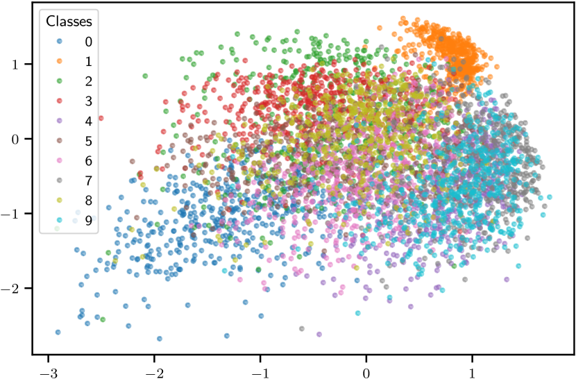
(a) Visualization of intermediate representations extracted from MNIST by using an auto-encoder. The intermediate feature vectors are in $\mathbb{R}^{2}$.

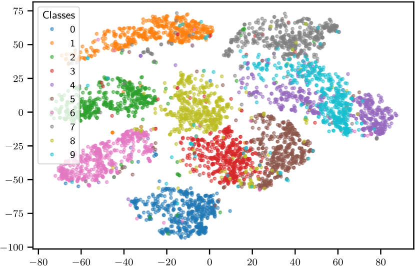
(b) We apply $t$-SNE to the intermediate feature vectors of an auto-encoder, which are in $\mathbb{R}^{16}$.

Figure 2: Two types of visualization of MNIST by using auto-encoders. Appendix A describes the details of visualization.

Reference	Domain	Visualization algorithm
Mikolov et al. [22]	NLP	PCA
Perozzi et al. [23]	Graph	Identity
Tang et al. [24]	Graph	$t$-SNE
Oord et al. [61]	Speech	$t$-SNE
Donahue et al. [62]	CV	$t$-SNE
Kornblith et al. [81]	CV	$t$-SNE
Islam et al. [115]	CV	$t$-SNE
Erhan et al. [118]	CV	Identity, ISOMAP
Medina et al. [135]	CV	$t$-SNE
Chuang et al. [137]	CV	$t$-SNE
Wang et al. [142]	CV	$t$-SNE
Tosh et al. [146]	NLP	$t$-SNE
Hashimoto et al. [148]	NLP	Identity
Wang and Isola [156]	CV	Identity
Kiros et al. [162]	NLP	$t$-SNE
Frosst et al. [178]	CV, Synsetic	Identity, $t$-SNE
Hadsell et al. [179]	CV	Identity
Garg and Liang [180]	Synsetic	$t$-SNE

Table 5: Summary of used visualization algorithms to extracted feature representations. Identity means the dimensionaility of extracted by a feature extractor is $2$ or $3$; the authors visualized the extracted feature vectors directly without a visualization algorithm.

Dimensionality reduction [181] maps a raw data sample into a lower-dimensional space such that the mapped representation preserves important information from the original data sample. For further details, please see general machine learning textbooks covering dimensionality reduction, for example, Shalev-Shwartz and Ben-David [182, Chapter 23], Murphy [183, Chapter 20], and the survey paper [181] who review $44$ dimensionality algorithms and compare them empirically from the visualization perspective.

The well known algorithms are independent component analysis [184], singular value decomposition, principal component analysis (PCA), LLE [185], Non-negative matrix factorization, $t$-distributed stochastic neighbor embedding ($t$-SNE) [186], and auto-encoder [84]. Representation learning works as dimensionality reduction when the dimensionality of extracted feature representation $d$ is smaller than the dimensionality of the original input $I$. Indeed, matrix factorization-based dimensionality reduction algorithms are compared with unsupervised representation learning to extract feature vectors, especially discrete data such as word [108, 150] and node [23, 24, 149]. Similarly, a contrastive loss [179] proposed for dimensionaility reduction is used as a loss function of representation learning.

Data visualization can be viewed as a special case of dimensionality reduction when extracted feature representations are in $\mathbb{R}^{2}$ or $\mathbb{R}^{3}$, where a human can recognize features visually. For example, for node representation learning, Perozzi et al. [23] showed feature vectors on $\mathbb{R}^{2}$ that representation learning extracts directly from a graph dataset. As a similar example, Fig. 2(a) shows intermediate feature representation of an auto-encoder trained on MNIST dataset. We also commonly apply a visualization algorithm to extracted feature representations $\big{\{}\widehat{{\mathbf{h}}}({\mathbf{x}}_{i})\big{\}}_{i=1}^{N_{D}}$ rather than directly learn feature representations in $\mathbb{R}^{2}$ or $\mathbb{R}^{3}$. For example, Mikolov et al. [22] visualized word vectors with PCA, and Donahue et al. [62] visualized feature vectors extracted by convolutional neural networks with $t$-SNE [186]. As a similar example, Fig. 2(b) shows $t$-SNE visualization of feature representations extracted an auto-encoder.

4.3.1 Experimental Procedure

Suppose $R$ pre-trained feature extractors $\{\widehat{{\mathbf{h}}}_{r}\}_{r=1}^{R}$ and downstream dataset ${\mathcal{D}}_{D}$. Extracted feature representations are denoted ${\mathcal{D}}_{D,r}=\{\widehat{{\mathbf{h}}}_{r}({\mathbf{x}}_{i})\}_{i=1}^{|{\mathcal{D}}_{D}|}$. We might not require the labels of ${\mathcal{D}}_{D}$ depending on the evaluation metric.

Dimensionality reduction

1. Extract feature representations with each feature extractor $\widehat{{\mathbf{h}}}_{r}$ from ${\mathcal{D}}_{D}$.

2. Compare sets of extracted representations ${\mathcal{D}}_{D,*}$ using evaluation metric for dimensionality reduction [181].

Visualization

1. Extract feature representations with each feature extractor $\widehat{{\mathbf{h}}}_{r}$ from ${\mathcal{D}}_{D}$.

2. If $d>3$, apply a dimensionality reduction algorithm to the feature representations ${\mathcal{D}}_{D,r}$ for visualization.

3. Compare visualized features with scatter plot.

4.3.2 Discussion

To our best knowledge, numerical evaluation of representation learning as dimensionality reduction is not performed commonly. However, investigating what information is implicitly embedded in learned representations is actively performed to understand representation learning algorithms. For example, given extracted sentence vectors, Adi et al. [177] trained a simple model to predict a property of a sentence, e.g., sentence length, the existence of a word, or order of two words, in order to understand sentence feature extractors. Intuitively, if the properties are embedded into extracted sentence vectors, the model can predict the properties accurately. Table 4 summarizes studies that evaluated representation learning algorithms from this perspective.

Numerical evaluation of visualization is challenging because it requires human evaluation, e.g., crowdsourcing [187]. We believe that this is why representation learning papers showed only generated figures without numerical evaluation on visualization. Another difficulty is that visualization algorithms generate different figures depending on their hyper-parameters. For example, $t$-SNE algorithm gives largely different visualization results depending on its hyper-parameters [188]. Hence we do not encourage evaluating representation learning algorithms using visualizations without careful the hyper-parameters tuning of visualization algorithms. Another approach is to use label information if we access a label of each sample by following $t$-SNE’s theoretical analysis [189]. In this case, we can use the similar evaluation protocol discussed in Section 4.1 with a simple classifier such as a linear classifier. Table 5 summarizes studies that evaluated representation learning algorithms with visualization.

4.4 Representation Learning as Auxiliary Task

This evaluation perspective differs from the others. We focus on a representation learning algorithm itself rather than pre-trained feature extractor $\widehat{{\mathbf{h}}}$. Since representation learning attempts to learn generic feature representations from a dataset, the representation learning algorithm might improve another machine learning algorithm’s performance by optimizing its loss and the loss of the downstream task simultaneously or cyclically, for example, in supervised [115, 178], semi-supervised learning [111, 190], few-shot learning [158], domain adaptation [191], and reinforcement learning [61]. Table 6 summarizes papers categorized into this evaluation perspective.

Reference	Main task	$L_{\mathrm{aux}}$	Dataset of $L_{\mathrm{aux}}$
Oord et al. [61]	Reinforcement learning	Contrastive [61]	S
Mitrovic et al. [94]	Reinforcement learning	Contrastive [94]	S
Chuang et al. [137]	Reinforcement learning	Contrastive [61]	S
Zhai et al. [90]	Source task of transfer learning	Either of [132, 159]	S, U
Zhai et al. [111]	Semi-supervised learning	Either of [132, 159]	U
Weston et al. [190]	Semi-supervised learning	Contrastive [179]	U
Gidaris et al. [158]	Pre-training of few-shot learning	Either of [132, 160]	S, U
Carlucci et al. [191]	Domain generalization, domain adaptation	Jigsaw [161]	S, Unl
Luong et al. [192]	Multi-task learning	Either of [162, 163]	Unl
Islam et al. [115]	Source task of transfer learning, Pre-training of Few-shot learning	Contrastive  [87]	S
Frosst et al. [178]	Supervised learning	Soft nearest neighbor loss [178]	S

Table 6: The categorized experimental settings in Section 4.4. For the dataset column, “S” stands for the same dataset as in the main task, “U” stands for an additional unlabeled dataset, and “Uni” stands for the union of the main task’s dataset and additional unlabeled dataset.

Suppose the same notations and classification formulation introduced in Section 4.1. Recall that we aim to learn a classifier that consists of feature extractor ${\mathbf{h}}_{D}$ and classification head ${\mathbf{g}}_{D}$ by minimizing supervised loss $L_{D}$, e.g., softmax cross-entropy loss (1). Let $L_{\mathrm{aux}}$ be a representation learning’s loss, e.g., mean squared loss (2) for an auto-encoder-based representation learning algorithm and ${\mathbf{g}}_{\mathrm{aux}}$ be a representation learning specific projection head, e.g., the decoder of the auto-encoder model. Suppose that the supervised and representation learning models share ${\mathbf{h}}_{D}$. For example, ${\mathbf{h}}_{D}$ is a convolutional neural network, and loss-specific heads ${\mathbf{g}}_{D}$ and ${\mathbf{g}}_{\mathrm{aux}}$ are different fully-connected layers. Formally, we optimize the following loss function to solve supervised loss $L_{\mathrm{D}}$ with representation learning loss $L_{\mathrm{aux}}$:

$$\min_{{\mathbf{h}}_{D},{\mathbf{g}}_{D},{\mathbf{g}}_{\mathrm{aux}}}L_{\mathrm{D}}({\mathbf{h}}_{D},{\mathbf{g}}_{D})+\beta L_{\mathrm{aux}}({\mathbf{h}}_{D},{\mathbf{g}}_{\mathrm{aux}}),$$ (14)

where pre-defined coefficient $\beta\in\mathbb{R}_{\geq 0}$. The feature extractor ${\mathbf{h}}_{D}$ can be released as a pre-trained feature extractor as the by-product of this supervised training [90, 158].

4.4.1 Experimental procedure

Suppose $R$ representation learning algorithms. For each representation learning algorithm, we optimize Eq. 14. We select the best one using the evaluation metric, such as validation accuracy for a classification task.

Variety of the dataset for representation learning

There exist several ways to calculate representation learning loss $L_{\mathrm{aux}}$. The simplest way is to use the same labeled dataset, $D_{D}$ [115, 178]. Other ways are to use an additional unlabeled dataset [192] or the union of labeled and unlabeled datasets [111, 190]. When we use an unlabeled dataset, the unlabeled dataset can come from the same data distribution [111] or a different data distribution [192].

4.4.2 Discussion

This formulation can be seen as a multi-task learning [193] whose tasks are the combination of a supervised task and a representation learning task. Compared with the other evaluation perspectives, this evaluation is easy to tune hyper-parameters of the representation learning algorithm because we can search the hyper-parameters in the single training stage since pre-training in Section 4.1 and regularization in Section 4.2 require two-stage training: training the representation learning model and training the model of the downstream task.

5 Theoretical Analyses of Representation Learning

To understand the empirical success of representation learning, theoretical analysis of representation learning is as important as an empirical evaluation because it could yield novel representation algorithms and justify the empirical observation or techniques. In this section, we mainly review theoretical analyses on unsupervised representation learning algorithms.

5.1 Relationship between Representation Learning and Downstream Tasks

The majority of theoretical approach shows an inequality using the losses of representation learning and downstream tasks. Loosely, given a feature extractor ${\mathbf{h}}$, the inequality is defined as

$$\widehat{L}_{D}({\mathbf{h}},{\mathbf{g}}_{D})\leq\alpha\widehat{L}_{\mathrm{un}}({\mathbf{h}},{\mathbf{g}})+\beta,$$ (15)

where $\alpha\in\mathbb{R}_{+}$ and $\beta\in\mathbb{R}$ are theorical analysis dependent terms. This inequality implies that minimization of the loss of the downstream task $\widehat{L}_{\mathrm{un}}$ implicitly minimizes the loss of the representation learning task $\widehat{L}_{D}$. The advantage of this type of inequality is that we can obtain generalization error bound in statistical learning theory [182] such as Rademacher complexity [110] and PAC-Bayes-based complexity [136].

5.1.1 Representation Learning Specific Analysis

Most existing theoretical work specifies a representation learning task, especially the loss function. We shall review the recent progress in this approach.

Contrastive loss with conditional independence.

Since contrastive loss [179] is a state-of-the-art representation learning objective over the last decade [22, 61], theoretical analysis on the contrastive loss is actively performed. Suppose we learn extractor ${\mathbf{h}}$ by minimzing a contrastive loss such as InfoNCE loss [61] on unsupervised dataset $D_{\mathrm{un}}$:

$$\widehat{L}_{\mathrm{cont}}({\mathbf{h}},{\mathbf{g}})=-\frac{1}{M}\sum_{i=1}^{M}\ln\frac{\exp\left[\mathrm{sim}({\mathbf{g}}({\mathbf{h}}({\mathbf{x}}_{i})),{\mathbf{g}}({\mathbf{h}}({\mathbf{x}}_{i}^{+})))\right]}{\exp\left[\mathrm{sim}({\mathbf{g}}({\mathbf{h}}({\mathbf{x}}_{i})),{\mathbf{g}}({\mathbf{h}}({\mathbf{x}}_{i}^{+})))\right]+\displaystyle{\sum_{k\in[K]}}\exp\left[\mathrm{sim}\left({\mathbf{g}}({\mathbf{h}}({\mathbf{x}}_{i})),{\mathbf{g}}\left({\mathbf{h}}\left({\mathbf{x}}_{(i,k)}^{-}\right)\right)\right)\right]},$$ (16)

where $\mathrm{sim}(.,.)$ is a similarity function, $\mathbb{R}^{O}\times\mathbb{R}^{O}\rightarrow\mathbb{R}$, such as dot product or cosine similarity. In Eq. 16, we need $K+1$ samples for each sample ${\mathbf{x}}_{i}$: positive sample ${\mathbf{x}}_{i}^{+}$ and $K$ negative samples $\{{\mathbf{x}}_{(i,k)}^{-}\}_{k=1}^{K}$ that are randomly drawn from the dataset $D_{\mathrm{un}}$.

Arora et al. [110] showed the first theoretical analysis for contrastive unsupervised representation learning with hinge and logistic losses. The key assumption of CURL is conditional independence on positive pair (${\mathbf{x}},{\mathbf{x}}^{+}$); given a latent class $c$, the positive pair is sampled by ${\mathbf{x}}_{i},{\mathbf{x}}_{i}^{+}\sim p({\mathbf{x}}\mid c)^{2}$. Note that latent class $c$ cannot be observed directly, and the latent class is related to the supervised class in the (unseen) downstream task. Under the same conditional independent assumptions, Nozawa et al. [136], Chuang et al. [137] extended the results for non-vacuous generalization bound and the debiasing of negative sampling, respectively. Similarly, Tosh et al. [164] weakened the assumption under $K=1$ and multi-view setting. Instead of assuming a latent class, Tosh et al. [164] introduced a latent variable that makes two views conditionally independent.

Contrastive loss with data-augmentation.

Since state-of-the-art unsupervised contrastive representation learning algorithms [65, 87, 88, 121] generate positive pairs by applying data-augmentation to the same sample, the conditional independence assumption does not hold for these algorithms. Relaxing the assumption is the main concern in theoretical analysis for contrastive unsupervised representation learning. Note that this analysis is still useful in similar machine learning formulations such as metric learning and SU learning [194] because this assumption holds naturally.

In Arora et al. [110, Section 6.2], a large number of negative samples $K$ in Eq. 16 have a negative impact on the downstream tasks because we are more likely to draw a negative sample ${\mathbf{x}}^{-}$ whose latent class $c^{-}$ is the same as one of the positive pair. On the contrary, recent contrastive representation learning algorithms [87, 121] reported that using large $K$ improves downstream performance in practice. To deal with this regime, Nozawa and Sato [114] showed large $K$ is necessary to approximate the loss of the downstream task by extending the results by Arora et al. [110] with the Coupon collector’s problem and without the conditional independent assumption. Similarly, Wang et al. [142] proposed a theoretical analysis that deals with the large $K$ regime and incorporates data-augmentation explicitly.

As another line of theoretical approach, Mitrovic et al. [94] showed conditions such that $\widehat{{\mathbf{h}}}$ generalizes to downstream tasks using a causal framework. Intuitively, feature extractor $\widehat{{\mathbf{h}}}$ needs to i) distinguish finer-grained classes than ones of downstream tasks to generalize the unseen downstream tasks and ii) be invariant under the change of a style that is not a relevant part of an image for downstream tasks. A contrastive loss [159] and data-augmentation are justified to satisfy the two conditions, respectively. HaoChen et al. [141] proposed spectral graph-based analysis without the conditional independence assumption. The authors consider a graph, where a node is an augmented data sample, and nodes are connected if they are generated from the data sample by data-augmentation. Under this setting, the loss function of graph decomposition is similar to softmax-based contrastive loss [61]. Jing et al. [168] discussed the problem of the dimensional collapse of extracted feature representations by investigating the optimization dynamics of InfoNCE loss minimization with shallow linear neural networks. Wen and Li [169] showed the importance of data-augmentation in contrastive learning on data generated by a sparse coding model with shallow ReLU neural networks.

Non-contrastive task

Beyond contrastive representation learning, there exist analyses on different representation learning tasks. For example, reconstruction-based representation learning tasks [138], multi-task supervised representation learning for few-shot learning [144], self-training with data-augmentation [140], vanilla language modeling [112], and masked language modeling [139]. Dubois et al. [157] proposed Decodable Information Bottleneck to guarantee supervised representation learning performance.

Representation learning with auxiliary loss

Theoretical analyses so far assume two stages of training as reviewed in Section 4.1. For one-stage training as described in Section 4.4, theoretical analyses also are performed. Le et al. [195] showed the stability bound of a supervised loss with a linear auto-encoder used for the auxiliary task. Similarly, Garg and Liang [180] proposed sample complexity bounds for unsupervised representation learning, which is a reconstruction-based task, and supervised learning losses. In their analysis, intuitively, representation learning can work as a learnable regularizer to reduce the hypothesis size of the supervised model. Maurer et al. [196] gave sample complexity bounds for multi-task supervised learning and learning-to-learn via shared feature extractor ${\mathbf{h}}_{D}$ for all tasks.

5.1.2 Representation Learning Agnostic Analysis

A few studies analyze a predictor on downstream tasks given a pre-trained feature extractor $\widehat{{\mathbf{h}}}$. The existing work showed the advantage of the frozen protocol with a linear classifier. Concretely, Bansal et al. [143] showed linear probing is more robust to the robustness of label corruption than fully-supervised way, and Kumar et al. [165] showed linear probing generalizes better to out-of-domain dataset than fine-tuning after fitting on a downstream dataset.

5.2 Optimality in Contrastive Representation Learning without Negative Samples

Contrastive learning without negative samples (NCL) such as [122, 167] is a novel type of unsupervised representation learning motivated by removing the negative samples in the contrastive loss (16). Even though NCL has collapsed minima: the outputs ${\mathbf{g}}({\mathbf{f}}(.))$ are the same constant vector, empirically, it performs competitively well as a feature extractor for the downstream tasks. Tian et al. [170] theoretically pointed out the importance of the stop-gradient technique and the existence of a projection head ${\mathbf{g}}$ to avoid such trivial solutions with linear neural networks. Pokle et al. [197] showed that NCL has non-collapsed bad global minima, which means minima are far from ground truth weights under shallow feature extractor without projection head and synthetic data based on sparse coding with random mask data-augmentation setting. On the other hand, contrastive unsupervised representation learning does not have such bad global minima. If we appropriately set initialization and normalization for the weights in a feature extractor, the NCL converges to the ground truth [197, Theorem 3]. Unlike theoretical analyses for contrastive representation learning in Section 5.1, these results do not give an inequality (15); revealing the relationship between the representation learning and downstream losses is worth interesting in exploring as a future direction.

5.3 Relation to Other Metrics

To understand what information is embedded by representation learning algorithms like Section 4.3, researchers show the equivalence of optimization representation learning and other metrics.

For discrete data, especially natural language processing, information-theoretic analyses are actively proposed. Levy and Goldberg [109] showed that skip-gram with negative sampling algorithm [22] implicitly decomposes a variant of point-wise mutual information (PMI) between word co-occurrence in the training corpus under assumptions, whose results are extended [151, 198]. Qiu et al. [152] extended the word embeddings results [109] to node representation learning algorithms. Similarly, Hashimoto et al. [148] showed that word embedding algorithm could be formulated as matrix recovery, where the matrix is a PMI matrix of word co-occurrence counts, and Arora et al. [153] showed similar results from a generative model perspective. Kong et al. [119] unified widely used algorithms in natural language processing from a mutual information perspective, including more recent models such as BERT [42]. Under the assumption of a generative model for documentations data, Tosh et al. [146] showed contrastive representation learning could recover the topic posterior of a document.

Beyond discrete data, a relation between representation learning loss function and mutual information is discussed. For example, contrastive loss function (16) can be interpreted as a lower bound of mutual information [61, 64, 199] or as an approximation of Hilbert-Schmidt independence criterion (HSIC) [154]. Note that tighter estimation of mutual information does not guarantee the generalization for the downstream task empirically [147, 155]. Complementary, Wang and Isola [156] showed an interpretation of the role of a contrastive loss on hyper-sphere representation space. Vincent [200] showned a connection between denoising autoencoder [106] and score matching [201] that is an efficient estimation method for probabilistic models.

6 Conclusion and Future Directions

Representation learning trains a feature extractor that automatically extracts generic feature representations from a dataset. Unlike existing representation learning survey papers, we reviewed four evaluation methods of representation learning algorithms to understand the current representation learning applications. We also reviewed theoretical work on representation learning. We conclude this review by discussing the future directions based on Vapnik’s principle [202].

A famous principle to solve a problem says

When solving a given problem, try to avoid solving a more general problem as an intermediate step. (Vapnik [202])

Regarding the common evaluations in representation learning, representation learning seems to oppose Vapnik’s principle. For example, suppose a binary image classification: dog versus cat, as a downstream task. We should not need a feature extractor that can distinguish the difference between Birman and Ragdoll, which are quite similar cat species, to solve the downstream task by following the principle. However, we impose such ability on representation learning because it learns the generic feature extractor from a massive dataset for unseen downstream tasks. In this sense, Vapnik’s principle is inapplicable to representation learning. Therefore we believe that we need a different metric to evaluate representation learning algorithms rather than the performance of a single downstream task, such as validation accuracy on ImageNet-1K. One possible solution is to measure the averaged performance among diverse downstream tasks, such as VTAB [90] for vision or SuperGLUE [13] for language. This idea can be generalized to modal-agnostic evaluation as discussed in Tamkin et al. [116].

More pessimistically, solving the downstream task via representation learning, especially two-stage training, is less effective than solving the problem directly with comprehensive hyper-parameter tuning. We expect the learned representations to capture redundant features to solve the downstream task, i.e., distinguishing between Birman and Ragdoll. Such unnecessary expressiveness could hurt downstream tasks’ performance. In transfer learning terminology, a negative transfer might cause this ineffectiveness. However, unsupervised representation learning has advantages compared with supervised learning, such as robustness to class imbalance [117] or generalization to unseen classes [93]. Hence we reach the same future direction as in the previous paragraph: can we develop suitable evaluation metrics rather than only a single metric of a downstream task for representation learning?

Appendix A Experimental Settings

We trained a neural network with a fully connected hidden layer on the training dataset of MNIST. We minimized a mean squared reconstruction error by using AdamW [203] whose learning rate was initialized by $0.01$. We adjusted the learning rate by using PyTorch [204]’s CosineAnnealingWarmRestarts [205] by epoch. The mini-batch size was $500$, and the number of epochs was $20$. As pre-processing, we normalized the input image.

We visualized feature vectors extracted by the hidden units on the validation dataset with Matplotlib [206]. We used only $500$ samples per class to avoid showing too dense visualizations. For Fig. 2(b), we applied $t$-SNE implemented by scikit-learn [207] with its default hyper-parameters to the extracted feature representations whose dimensionality was $16$. We developed the experimental codes on Jupyter Notebook [208].

References

- Nozawa and Sato [2022] Kento Nozawa and Issei Sato. Evaluation Methods for Representation Learning: A Survey. In IJCAI-ECAI Survey Track, 2022.
- Goodfellow et al. [2016] Ian Goodfellow, Yoshua Bengio, and Aaron Courville. Deep Learning. MIT Press, 2016. URL https://www.deeplearningbook.org.
- Krizhevsky et al. [2012] Alex Krizhevsky, Ilya Sutskever, and Geoffrey E. Hinton. ImageNet Classification with Deep Convolutional Neural Networks. In NeurIPS, pages 1097–1105, 2012.
- Ronneberger et al. [2015] Olaf Ronneberger, Philipp Fischer, and Thomas Brox. U-Net: Convolutional Networks for Biomedical Image Segmentation. In MICCAI, pages 234–241, 2015.
- Kingma and Welling [2014] Diederik P. Kingma and Max Welling. Auto-Encoding Variational Bayes. In ICLR, 2014.
- Goodfellow et al. [2014] Ian J. Goodfellow, Jean Pouget-Abadie, Mehdi Mirza, Bing Xu, David Warde-Farley, Sherjil Ozair, Aaron Courville, and Yoshua Bengio. Generative Adversarial Nets. In NeurIPS, pages 2672–2680, 2014.
- Vaswani et al. [2017] Ashish Vaswani, Noam Shazeer, Niki Parmar, Jakob Uszkoreit, Llion Jones, Aidan N. Gomez, Łukasz Kaiser, and Illia Polosukhin. Attention Is All You Need. In NeurIPS, pages 5998–6008, 2017.
- Hinton et al. [2012] Geoffrey Hinton, Li Deng, Dong Yu, George E. Dahl, Abdel-rahman Mohamed, Navdeep Jaitly, Andrew Senior, Vincent Vanhoucke, Patrick Nguyen, Tara N. Sainath, and Brian Kingsbury. Deep Neural Networks for Acoustic Modeling in Speech Recognition. IEEE Signal Processing Magazine, 29(6):82–97, 2012.
- Mnih et al. [2015] Volodymyr Mnih, Koray Kavukcuoglu, David Silver, Andrei A. Rusu, Joel Veness, Marc G. Bellemare, Alex Graves, Martin Riedmiller, Andreas K. Fidjeland, Georg Ostrovski, Stig Petersen, Charles Beattie, Amir Sadik, Ioannis Antonoglou, Helen King, Dharshan Kumaran, Daan Wierstra, Shane Legg, and Demis Hassabis. Human-level Control through Deep Reinforcement Learning. Nature, 518(7540):529–533, 2015.
- He et al. [2016] Kaiming He, Xiangyu Zhang, Shaoqing Ren, and Jian Sun. Deep Residual Learning for Image Recognition. In CVPR, pages 770–778, 2016.
- Deng et al. [2009] Jia Deng, Wei Dong, Richard Socher, Li-Jia Li, Kai Li, and Li Fei-Fei. ImageNet: A Large-Scale Hierarchical Image Database. In CVPR, pages 248–255, 2009.
- He et al. [2021a] Pengcheng He, Xiaodong Liu, Jianfeng Gao, and Weizhu Chen. DeBERTa: Decoding-enhanced BERT with Disentangled Attention. In ICLR, 2021a.
- Wang et al. [2019] Alex Wang, Yada Pruksachatkun, Nikita Nangia, Amanpreet Singh, Julian Michael, Felix Hill, Omer Levy, and Samuel R. Bowman. SuperGLUE: A Stickier Benchmark for General-Purpose Language Understanding Systems. In NeurIPS, pages 3266–3280, 2019.
- Shawe-Taylor and Cristianini [2004] John Shawe-Taylor and Nello Cristianini. Kernel Methods for Pattern Analysis. 2004.
- LeCun et al. [1998] Yann LeCun, Léon Bottou, Yoshua Bengio, and Patrick Haffner. Gradient-Based Learning Applied to Document Recognition. Proceedings of the IEEE, 86:2278–2324, 1998.
- Perronnin et al. [2010] Florent Perronnin, Jorge Sánchez, and Thomas Mensink. Improving the Fisher Kernel for Large-Scale Image Classification. In ECCV, pages 143–156, 2010.
- Lowe [2004] David G. Lowe. Distinctive Image Feature from Scale-Invariant Keypoints. International Journal of Computer Vision, 60:91–110, 2004.
- LeCun et al. [2015] Yann LeCun, Yoshua Bengio, and Geoffrey Hinton. Deep learning. Nature, 521(7553):436–444, 2015.
- Bengio et al. [2013] Yoshua Bengio, Aaron Courville, and Pascal Vincent. Representation Learning: A Review and New Perspectives. IEEE Transactions on Pattern Analysis and Machine Intelligence, 35(8):1798–1828, 2013.
- Zhong et al. [2016] Guoqiang Zhong, Li-Na Wang, Xiao Ling, and Junyu Dong. An Overview on Data Representation Learning: From Traditional Feature Learning to Recent Deep Learning. The Journal of Finance and Data Science, 2(4):265–278, 2016.
- Mikolov et al. [2013a] Tomas Mikolov, Kai Chen, Greg Corrado, and Jeffrey Dean. Efficient Estimation of Word Representations in Vector Space. In ICLR Workshop, 2013a.
- Mikolov et al. [2013b] Tomas Mikolov, Ilya Sutskever, Kai Chen, Greg Corrado, and Jeffrey Dean. Distributed Representations of Words and Phrases and their Compositionality. In NeurIPS, pages 3111–3119, 2013b.
- Perozzi et al. [2014] Bryan Perozzi, Rami Al-Rfou, and Steven Skiena. DeepWalk: Online Learning of Social Representations. In KDD, pages 701–710, 2014.
- Tang et al. [2015] Jian Tang, Meng Qu, Mingzhe Wang, Ming Zhang, Jun Yan, and Qiaozhu Mei. LINE: Large-scale Information Network Embedding. In WWW, pages 1067–1077, 2015.
- Hamilton et al. [2017] William L. Hamilton, Rex Ying, and Jure Leskovec. Representation Learning on Graphs: Methods and Applications. IEEE Data Engineering Bulletin, 40(3):52–74, 2017.
- Goyal and Ferrara [2018] Palash Goyal and Emilio Ferrara. Graph Embedding Techniques, Applications, and Performance: A Survey. Knowledge-Based Systems, 151(1):78–94, 2018.
- Cai et al. [2018] Hongyun Cai, Vincent W. Zheng, and Kevin Chen-Chuan Chang. A Comprehensive Survey of Graph Embedding: Problems, Techniques and Applications. IEEE Transactions on Knowledge and Data Engineering, 30(9):1616–1637, 2018.
- Chen et al. [2020a] Fenxiao Chen, Yun Cheng Wang, Bin Wang, and C.-C. Jay Kuo. Graph Representation Learning: A Survey. APSIPA Transactions on Signal and Information Processing, 9:1–17, 2020a.
- Zhang et al. [2020] Daokun Zhang, Jie Yin, Xingquan Zhu, and Chengqi Zhang. Network Representation Learning: A Survey. IEEE Transactions on Big Data, 6:3–28, 2020.
- Kazemi et al. [2020] Seyed Mehran Kazemi, Rishab Goel, Kshitij Jain, Ivan Kobyzev, Akshay Sethi, Peter Forsyth, and Pascal Poupart. Representation Learning for Dynamic Graphs: A Survey. Journal of Machine Learning Research, 21:1–73, 2020.
- Hamilton [2020] William L. Hamilton. Graph Representation Learning. Morgan & Claypool, 2020. URL https://www.cs.mcgill.ca/~wlh/grl_book/.
- Lirong et al. [2021] Wu Lirong, Haitao Lin, Zhangyang Gao, Cheng Tan, and Stan Z. Li. Self-supervised on Graphs: Contrastive, Generative, or Predictive. arXiv:2105.07342v3 [cs.LG], 2021.
- Wang et al. [2017] Quan Wang, Zhendong Mao, Bin Wang, and Li Guo. Knowledge Graph Embedding: A Survey of Approaches and Applications. IEEE Transactions on Knowledge and Data Engineering, 29(12):2724–2743, 2017.
- Lin et al. [2018] Yankai Lin, Xu Han, Ruobing Xie, Zhiyuan Liu, and Maosong Sun. Knowledge Representation Learning: A Quantitative Review. arXiv:1812.10901v1 [cs.CL], 2018.
- Ji et al. [2022] Shaoxiong Ji, Shirui Pan, Erik Cambria, Pekka Marttinen, and Philip S. Yu. A Survey on Knowledge Graphs: Representation, Acquisition, and Applications. IEEE Transactions on Neural Networks and Learning Systems, 33(2):494–514, 2022.
- Smith [2020] Noah A. Smith. Contextual Word Representations: Putting Words into Computers. Communications of the ACM, 63(6):66–74, 2020.
- Eisenstein [2019] Jacob Eisenstein. Introduction to Natural Language Processing. Adaptive Computation and Machine Learning series. MIT Press, 2019. URL https://cseweb.ucsd.edu/~nnakashole/teaching/eisenstein-nov18.pdf.
- Liu et al. [2020] Zhiyuan Liu, Yankai Lin, and Maosong Sun. Representation Learning for Natural Language Processing. Springer, 2020.
- Rethmeier and Augenstein [2021] Nils Rethmeier and Isabelle Augenstein. A Primer on Contrastive Pretraining in Language Processing: Methods, Lessons Learned and Perspectives. arXiv:2102.12982v1 [cs.CL], 2021.
- Rogers et al. [2020] Anna Rogers, Olga Kovaleva, and Anna Rumshisky. A Primer in BERTology: What we Know about how BERT Works. Transactions of the Association for Computational Linguistics, 8:842–866, 2020.
- Xia et al. [2020] Patrick Xia, Shijie Wu, and Benjamin Van Durme. Which *BERT? A Survey Organizing Contextualized Encoders. In EMNLP, pages 7516–7533, 2020.
- Devlin et al. [2019] Jacob Devlin, Ming-Wei Chang, Kenton Lee, and Kristina Toutanova. BERT: Pre-training of Deep Bidirectional Transformers for Language Understanding. In NAACL-HLT, pages 4171–4186, 2019.
- Schnabel et al. [2015] Tobias Schnabel, Igor Labutov, David Mimno, and Thorsten Joachims. Evaluation Methods for Unsupervised Word Embeddings. In EMNLP, pages 298–307, 2015.
- Wallach et al. [2009] Hanna M. Wallach, Lain Murray, Ruslan Salakhutdinov, and David Mimno. Evaluation Methods for Topic Models. In ICML, pages 1105–1112, 2009.
- Guo et al. [2019] Wenzhong Guo, Jianwen Wang, and Shiping Wang. Deep Multimodal Representation Learning: A Survey. IEEE Access, 7:63373–63394, 2019.
- Li et al. [2019] Yingming Li, Ming Yang, and Zhongfei Zhang. A Survey of Multi-View Representation Learning. IEEE Transactions on Knowledge and Data Engineering, 31(10):1863–1883, 2019.
- Radford et al. [2021] Alec Radford, Jong Wook Kim, Chris Hallacy, Aditya Ramesh, Gabriel Goh, Sandhini Agarwal, Girish Sastry, Amanda Askell, Pamela Mishkin, Jack Clark, Gretchen Krueger, and Ilya Sutskever. Learning Transferable Visual Models From Natural Language Supervision. In ICML, pages 8748–8763, 2021.
- Le-Khac et al. [2020] Phuc H. Le-Khac, Graham Healy, and Alan F. Smeaton. Contrastive Representation Learning: A Framework and Review. IEEE Access, 8:193907–193934, 2020.
- Jaiswal et al. [2021] Ashish Jaiswal, Ashwin Ramesh Babu, Mohammad Zaki Zadeh, Debapriya Banerjee, and Fillia Makedon. A Survey on Contrastive Self-Supervised Learning. Technologies, 9(1), 2021.
- Jing and Tian [2019] Longlong Jing and Yingli Tian. Self-supervised Visual Feature Learning with Deep Neural Networks: A Survey. IEEE Transactions on Pattern Analysis and Machine Intelligence, 43:4037–4058, 2019.
- Schmarje et al. [2021] Lars Schmarje, Monty Santarossa, Simon-Martin Schröder, and Reinhard Koch. A Survey on Semi-, Self-and Unsupervised Learning in Image Classification. IEEE Access, 9:82146–82168, 2021.
- Huang et al. [2021] Gabriel Huang, Issam Laradji, David Vazquez, Simon Lacoste-Julien, and Pau Rodriguez. A Survey of Self-Supervised and Few-Shot Object Detection. arXiv:2110.14711 [cs], 2021.
- Weng and Kim [2021] Lilian Weng and Jong Wook Kim. Self-Supervised Learning: Self-Prediction and Contrastive Learning, Dec. 2021. URL https://neurips.cc/virtual/2021/tutorial/21895. NeurIPS Tutorial.
- Chapelle et al. [2006] Olivier Chapelle, Bernhard Schölkopf, and Alexander Zien. Semi-supervised Learning. MIT Press, 2006.
- Pan and Yang [2010] Sinno Jialin Pan and Qiang Yang. A Survey on Transfer Learning. IEEE Transactions on Knowledge and Data Engineering, 22(10):1345–1359, 2010.
- Weiss et al. [2016] Karl Weiss, Taghi M. Khoshgoftaar, and Dingding Wang. A Survey of Transfer Learning. Journal of Big Data, 3(1):1–40, 2016.
- Redko et al. [2020] Ievgen Redko, Emilie Morvant, Amaury Habrard, Marc Sebban, and Younès Bennani. A Survey on Domain Adaptation Theory. arXiv:2004.11829v5 [cs.LG], 2020.
- Kulis [2012] Brian Kulis. Metric Learning: A Survey. Foundations and Trends® in Machine Learning, 5(4):287–364, 2012.
- Bellet et al. [2014] Aurélien Bellet, Amaury Habrard, and Marc Sebban. A Survey on Metric Learning for Feature Vectors and Structured Data. arXiv:1306.6709v4 [cs.LG], 2014.
- Sohn [2016] Kihyuk Sohn. Improved Deep Metric Learning with Multi-class N-pair Loss Objective. In NeurIPS, pages 1857–1865, 2016.
- Oord et al. [2018] Aaron van den Oord, Yazhe Li, and Oriol Vinyals. Representation Learning with Contrastive Predictive Coding. arXiv:1807.03748v2 [cs.LG], 2018.
- Donahue et al. [2014] Jeff Donahue, Yangqing Jia, Oriol Vinyals, Judy Hoffman, Ning Zhang, Eric Tzeng, and Trevor Darrell. DeCAF: A Deep Convolutional Activation Feature for Generic Visual Recognition. In ICML, pages 647–655, 2014.
- Yosinski et al. [2014] Jason Yosinski, Jeff Clune, Yoshua Bengio, and Hod Lipson. How Transferable Are Features in Deep Neural Networks? In NeurIPS, pages 3320–3328, 2014.
- Hjelm et al. [2019] R Devon Hjelm, Alex Fedorov, Samuel Lavoie-Marchildon, Karan Grewal, Phil Bachman, Adam Trischler, and Yoshua Bengio. Learning Deep Representations by Mutual Information Estimation and Maximization. In ICLR, 2019.
- Bachman et al. [2019] Philip Bachman, R Devon Hjelm, and William Buchwalter. Learning Representations by Maximizing Mutual Information Across Views. In NeurIPS, pages 15535–15545, 2019.
- Baevski et al. [2021] Alexei Baevski, Wei-Ning Hsu, Alexis Conneau, and Michael Auli. Unsupervised Speech Recognition. In NeurIPS, pages 27826–27839, 2021.
- Abu-El-Haija et al. [2016] Sami Abu-El-Haija, Nisarg Kothari, Joonseok Lee, Paul Natsev, George Toderici, Balakrishnan Varadarajan, and Sudheendra Vijayanarasimhan. YouTube-8M: A Large-Scale Video Classification Benchmark. arXiv:1609.08675v1 [cs.CV], 2016.
- Conneau et al. [2017] Alexis Conneau, Douwe Kiela, Holger Schwenk, Loïc Barrault, and Antoine Bordes. Supervised Learning of Universal Sentence Representations from Natural Language Inference Data. In EMNLP, pages 670–680, 2017.
- Bowman et al. [2015] Samuel R. Bowman, Gabor Angeli, Christopher Potts, and Christopher D. Manning. A Large Annotated Corpus for Learning Natural Language Inference. In EMNLP, pages 632–642, 2015.
- McCann et al. [2017] Bryan McCann, James Bradbury, Caiming Xiong, and Richard Socher. Learned in Translation: Contextualized Word Vectors. In NeurIPS, pages 6297–6308, 2017.
- Simonyan and Zisserman [2015] Karen Simonyan and Andrew Zisserman. Very Deep Convolutional Networks for Large-Scale Image Recognition. In ICLR, 2015.
- Long et al. [2015] Jonathan Long, Evan Shelhamer, and Trevor Darrell. Fully Convolutional Networks for Semantic Segmentation. In CVPR, pages 3431–3440, 2015.
- Girshick et al. [2014] Ross Girshick, Jeff Donahue, Trevor Darrell, and Jitendra Malik. Rich Feature Hierarchies for Accurate Object Detection and Semantic Segmentation. In CVPR, pages 580–587, 2014.
- Girshick [2015] Ross Girshick. Fast R-CNN. In ICCV, pages 1440–1448, 2015.
- Ren et al. [2015] Shaoqing Ren, Kaiming He, Ross Girshick, and Jian Sun. Faster R-CNN: Towards Real-Time Object Detection with Region Proposal Networks. In NeurIPS, pages 91–99, 2015.
- Sun et al. [2017] Chen Sun, Abhinav Shrivastava, Saurabh Singh, and Abhinav Gupta. Revisiting Unreasonable Effectiveness of Data in Deep Learning Era. In ICCV, pages 843–852, 2017.
- Mahajan et al. [2018] Dhruv Mahajan, Ross Girshick, Vignesh Ramanathan, Kaiming He, Manohar Paluri, Yixuan Li, Ashwin Bharambe, and Laurens van der Maaten. Exploring the Limits of Weakly Supervised Pretraining. In ECCV, pages 185–201, 2018.
- Kolesnikov et al. [2020] Alexander Kolesnikov, Lucas Beyer, Xiaohua Zhai, Joan Puigcerver, Jessica Yung, Sylvain Gelly, and Neil Houlsby. Big Transfer (BiT): General Visual Representation Learning. In ECCV, pages 491–507, 2020.
- Kataoka et al. [2020] Hirokatsu Kataoka, Kazushige Okayasu, Asato Matsumoto, Eisuke Yamagata, Ryosuke Yamada, Nakamasa Inoue, Akio Nakamura, and Yutaka Satoh. Pre-training without Natural Images. In ACCV, 2020.
- Beyer et al. [2020] Lucas Beyer, Olivier J. Hénaff, Alexander Kolesnikov, Xiaohua Zhai, and Aäron van den Oord. Are We Done with ImageNet? arXiv:2006.07159v1 [cs.CV], 2020.
- Kornblith et al. [2019] Simon Kornblith, Jonathon Shlens, and Quoc V. Le. Do Better ImageNet Models Transfer Better? In CVPR, pages 2661–2671, 2019.
- Abnar et al. [2022] Samira Abnar, Mostafa Dehghani, Behnam Neyshabur, and Hanie Sedghi. Exploring the Limits of Large Scale Pre-training. In ICLR, 2022.
- Ericsson et al. [2021] Linus Ericsson, Henry Gouk, and Timothy M. Hospedales. How Well Do Self-Supervised Models Transfer? In CVPR, pages 5414–5423, 2021.
- Rumelhart et al. [1986] David E. Rumelhart, Geoffrey E. Hinton, and Ronald J. Williams. Learning Internal Representations by Error Propagation. In Parallel Distributed Processing: Explorations in the Microstructure of Cognition: Foundations, pages 318–362. MIT Press, 1986.
- Mikolov et al. [2018] Tomas Mikolov, Edouard Grave, Piotr Bojanowski, Christian Puhrsch, and Armand Joulin. Advances in Pre-Training Distributed Word Representations. In LREC, pages 52–55, 2018.
- Du et al. [2021a] Nan Du, Yanping Huang, Andrew M. Dai, Simon Tong, Dmitry Lepikhin, Yuanzhong Xu, Maxim Krikun, Yanqi Zhou, Adams Wei Yu, Orhan Firat, Barret Zoph, Liam Fedus, Maarten Bosma, Zongwei Zhou, Tao Wang, Yu Emma Wang, Kellie Webster, Marie Pellat, Kevin Robinson, Kathy Meier-Hellstern, Toju Duke, Lucas Dixon, Kun Zhang, Quoc V. Le, Yonghui Wu, Zhifeng Chen, and Claire Cui. GLaM: Efficient Scaling of Language Models with Mixture-of-Experts. arXiv:2112.06905v1 [cs.CL], 2021a.
- He et al. [2020] Kaiming He, Haoqi Fan, Yuxin Wu, Saining Xie, and Ross Girshick. Momentum Contrast for Unsupervised Visual Representation Learning. In CVPR, pages 9726–9735, 2020.
- Caron et al. [2020] Mathilde Caron, Ishan Misra, Julien Mairal, Priya Goyal, Piotr Bojanowski, and Armand Joulin. Unsupervised Learning of Visual Features by Contrasting Cluster Assignments. In NeurIPS, pages 9912–9924, 2020.
- Goyal et al. [2021] Priya Goyal, Mathilde Caron, Benjamin Lefaudeux, Min Xu, Pengchao Wang, Vivek Pai, Mannat Singh, Vitaliy Liptchinsky, Ishan Misra, Armand Joulin, and Piotr Bojanowski. Self-supervised Pretraining of Visual Features in the Wild. arXiv:2103.01988v2, 2021.
- Zhai et al. [2020] Xiaohua Zhai, Joan Puigcerver, Alexander Kolesnikov, Pierre Ruyssen, Carlos Riquelme, Mario Lucic, Josip Djolonga, Andre Susano Pinto, Maxim Neumann, Alexey Dosovitskiy, Lucas Beyer, Olivier Bachem, Michael Tschannen, Marcin Michalski, Olivier Bousquet, Sylvain Gelly, and Neil Houlsby. A Large-scale Study of Representation Learning with the Visual Task Adaptation Benchmark. arXiv:1910.04867v2 [cs.CV], 2020.
- Hernandez et al. [2021] Danny Hernandez, Jared Kaplan, Tom Henighan, and Sam McCandlish. Scaling Laws for Transfer. arXiv:2102.01293v1 [cs.LG], 2021.
- Kotar et al. [2021] Klemen Kotar, Gabriel Ilharco, Ludwig Schmidt, Kiana Ehsani, and Roozbeh Mottaghi. Contrasting Contrastive Self-Supervised Representation Learning Pipelines. In ICCV, pages 9949–9959, 2021.
- Sariyildiz et al. [2021] Mert Bulent Sariyildiz, Yannis Kalantidis, Diane Larlus, and Karteek Alahari. Concept Generalization in Visual Representation Learning. In ICCV, pages 9629–9639, 2021.
- Mitrovic et al. [2021] Jovana Mitrovic, Brian McWilliams, Jacob Walker, Lars Buesing, and Charles Blundell. Representation Learning via Invariant Causal Mechanisms. In ICLR, 2021.
- Kolesnikov et al. [2019] Alexander Kolesnikov, Xiaohua Zhai, and Lucas Beyer. Revisiting Self-Supervised Visual Representation Learning. In CVPR, pages 1920–1929, 2019.
- Hinton et al. [1986] Geoffrey E. Hinton, James. L. McClelland, and David E. Rumelhart. Distributed Representations. In Parallel Distributed Processing: Explorations in the Microstructure of Cognition: Foundations, pages 77–109. MIT Press, 1986.
- Turing [1950] Alan M. Turing. Computing Machinery and Intelligence. Mind, LIX:433–460, 1950.
- Fisher [1936] Ronald A. Fisher. The Use of Multiple Measurements in Taxonomic Problems. Annals of Eugenics, 7(2):179–188, 1936.
- Bengio et al. [2003] Yoshua Bengio, Réjean Ducharme, Pascal Vincent, and Christian Jauvin. A Neural Probabilistic Language Model. Journal of machine learning research: JMLR, 3:1137–1155, 2003.
- Hutter et al. [2019] Frank Hutter, Lars Kotthoff, and Joaquin Vanschoren, editors. Automated Machine Learning - Methods, Systems, Challenges. Springer, 2019.
- Elsken et al. [2019] Thomas Elsken, Jan Hendrik Metzen, and Frank Hutter. Neural Architecture Search: A Survey. Journal of Machine Learning Research, 20(55):1–21, 2019.
- Ranzato et al. [2006] Marc’Aurelio Ranzato, Christopher Poultney, Sumit Chopra, and Yann LeCun. Efficient Learning of Sparse Representations with an Energy-Based Model. In NeurIPS, pages 1137–1144, 2006.
- Higgins et al. [2018] Irina Higgins, David Amos, David Pfau, Sebastien Racaniere, Loic Matthey, Danilo Rezende, and Alexander Lerchner. Towards a Definition of Disentangled Representations. arXiv:1812.02230v1, 2018.
- Dehghani et al. [2022] Mostafa Dehghani, Anurag Arnab, Lucas Beyer, Ashish Vaswani, and Yi Tay. The Efficiency Misnomer. In ICLR, 2022.
- Hinton et al. [2006] Geoffrey E. Hinton, Simon Osindero, and Yee-Whye Teh. A Fast Learning Algorithm for Deep Belief Nets. Neural Computation, 18:1527–1554, 2006.
- Vincent et al. [2008] Pascal Vincent, Hugo Larochelle, Yoshua Bengio, and Pierre-Antoine Manzagol. Extracting and Composing Robust Features with Denoising Autoencoders. In ICML, pages 1096–1103, 2008.
- Hénaff et al. [2020] Olivier J. Hénaff, Aravind Srinivas, Jeffrey De Fauw, Ali Razavi, Carl Doersch, S. M. Ali Eslami, and Aaron van den Oord. Data-Efficient Image Recognition with Contrastive Predictive Coding. In ICML, pages 4182–4192, 2020.
- Baroni et al. [2014] Marco Baroni, Georgiana Dinu, and Germán Kruszewski. Don’t Count, Predict! A Systematic Comparison of Context-counting vs. Context-predicting Semantic Vectors. In ACL, pages 238–247, 2014.
- Levy and Goldberg [2014] Omer Levy and Yoav Goldberg. Neural Word Embedding as Implicit Matrix Factorization. In NeurIPS, pages 2177–2185, 2014.
- Arora et al. [2019] Sanjeev Arora, Hrishikesh Khandeparkar, Mikhail Khodak, Orestis Plevrakis, and Nikunj Saunshi. A Theoretical Analysis of Contrastive Unsupervised Representation Learning. In ICML, pages 5628–5637, 2019.
- Zhai et al. [2019] Xiaohua Zhai, Avital Oliver, Alexander Kolesnikov, and Lucas Beyer. S4L: Self-Supervised Semi-Supervised Learning. In ICCV, pages 1476–1485, 2019.
- Saunshi et al. [2021] Nikunj Saunshi, Sadhika Malladi, and Sanjeev Arora. A Mathematical Exploration of Why Language Models Help Solve Downstream Tasks. In ICLR, 2021.
- Zhao et al. [2021] Nanxuan Zhao, Zhirong Wu, Rynson W.H. Lau, and Stephen Lin. What Makes Instance Discrimination Good for Transfer Learning? In ICLR, 2021.
- Nozawa and Sato [2021] Kento Nozawa and Issei Sato. Understanding Negative Samples in Instance Discriminative Self-supervised Representation Learning. In NeurIPS, pages 5784–5797, 2021.
- Islam et al. [2021] Ashraful Islam, Chun-Fu Richard Chen, Rameswar Panda, Leonid Karlinsky, Richard Radke, and Rogerio Feris. A Broad Study on the Transferability of Visual Representations with Contrastive Learning. In ICCV, pages 8845–8855, 2021.
- Tamkin et al. [2021] Alex Tamkin, Vincent Liu, Rongfei Lu, Daniel Fein, Colin Schultz, and Noah Goodman. DABS: a Domain-Agnostic Benchmark for Self-Supervised Learning. In NeurIPS Datasets and Benchmarks Track, 2021. URL https://github.com/alextamkin/dabs.
- Liu et al. [2022] Hong Liu, Jeff Z. HaoChen, Adrien Gaidon, and Tengyu Ma. Self-supervised Learning is More Robust to Dataset Imbalance. In ICLR, 2022.
- Erhan et al. [2010] Dumitru Erhan, Yoshua Bengio, Aaron Courville, Pierre-Antoine Manzagol, Pascal Vincent, and Samy Bengio. Why Does Unsupervised Pre-training Help Deep Learning? Journal of Machine Learning Research, 11:625–660, 2010.
- Kong et al. [2020] Lingpeng Kong, Cyprien de Masson D’Autume, Wang Ling, Lei Yu, Zihang Dai, and Dani Yogatama. A Mutual Information Maximization Perspective of Language Representation Learning. In ICLR, 2020.
- Wieting and Kiela [2019] John Wieting and Douwe Kiela. No Training Required: Exploring Random Encoders for Sentence Classification. In ICLR, 2019.
- Chen et al. [2020b] Ting Chen, Simon Kornblith, Mohammad Norouzi, and Geoffrey Hinton. A Simple Framework for Contrastive Learning of Visual Representations. In ICML, pages 1597–1607, 2020b.
- Grill et al. [2020] Jean-Bastien Grill, Florian Strub, Florent Altché, Corentin Tallec, Pierre H. Richemond, Elena Buchatskaya, Carl Doersch, Bernardo Avila Pires, Zhaohan Daniel Guo, Mohammad Gheshlaghi Azar, Bilal Piot, Koray Kavukcuoglu, Rémi Munos, and Michal Valko. Bootstrap Your Own Latent A New Approach to Self-Supervised Learning. In NeurIPS, pages 21271–21284, 2020.
- He et al. [2021b] Kaiming He, Xinlei Chen, Saining Xie, Yanghao Li, Piotr Dollár, and Ross Girshick. Masked Autoencoders Are Scalable Vision Learners. arXiv:2111.06377v3 [cs], 2021b.
- Newell and Deng [2020] Alejandro Newell and Jia Deng. How Useful is Self-Supervised Pretraining for Visual Tasks? In CVPR, pages 7345–7354, 2020.