Axion-Like Particle Interpretation of Dark Matter and Muon $(g-2)$

Abstract

We investigate the dark matter (DM) phenomenology of axion-like particles (ALP) along with the ALP interpretation of muon $(g-2)$ in a minimal extension of the Standard Model (SM). Here we have considered flavor dependent ALP couplings with SM leptons to study the allowed region of parameter space from the muon $(g-2)$ measurement, taking into account all possible one and two loop diagrams. We have found that in a certain region of parameter space ALP can act as a DM, satisfying the constraint from muon $(g-2)$ and other experimental bounds. From our relic density calculation, we can infer that the ALP can act as a DM candidate in the mass range between ${55\rm MeV}$ to $100{\rm MeV}$ while satisfying muon $(g-2)$ observation and other experimental constraints.

I Introduction

The precise measurement of the anomalous magnetic moment of muon reveals the possibility of existing physics beyond Standard Model (BSM). Combining the old measurement of muon $(g-2)$ by BNL E821 experiment [1] along with the recent one by Fermilab [2], it was observed that the experimental observation of $a_{\mu}(\equiv(g-2)/2)$ differs with the Standard Model (SM) prediction by $4.2\sigma$ and the deviation is given by [2]

$$\Delta a_{\mu}=(251\pm 59)\times 10^{-11}\,\,\,.$$

The apparent mismatch between theoretical prediction [3] and experimental observation may be a pointer towards the physics beyond the Standard Model and people have proposed many new ideas to address this issue [4, 5, 6].

Another, prima facie unrelated, issue of the SM is the appearance of a CP violating phase ($\theta_{\rm QCD}$) in the quantum chromodynamics (QCD) Lagrangian [7, 8] which has to be tightly constrained from the measurement of neutron electric dipole moment and the upper bound of $\theta_{\rm QCD}$ is $10^{-10}$ [9]. The problem of tiny value of $\theta_{\rm QCD}$ has been resolved by proposing a new axial $U(1)$ global symmetry, known as Pecci-Quinn (PQ) symmetry [10, 11]. In this scenario, $\theta_{\rm QCD}$ parameter is replaced by a dynamical field, known as axion [12, 13]. The axion field generates tiny mass from the QCD non-perturbative effects and it can act as a dark matter (DM) candidate [14, 15, 16, 17, 18]. It is to be noted that the mass of axion and its coupling with SM are not free parameters because both of them are functions of the PQ breaking scale.

Generalising the idea of axion, one can also consider axion-like particles (ALP) which is a pseudo Nambu-Goldstone boson, appearing in the theory due to the spontaneous breaking of an approximate global symmetry. The motivations of proposing such ALP are some high scale scenario such as string theory [19, 20]. An ALP has rich phenomenological implications since its mass and couplings with the SM fields are independent parameters, in contrast to a PQ axion [21, 22, 23, 24]. The couplings of ALP with the SM fields are similar to that of an axion which implies that the ALP couples with two photon via a dimension five operator and it can decay into two photon. The coupling of ALP with photon has very rich phenomenology and it can be constrained from various laboratory, astrophysical observations as discussed in [28, 29, 26, 21, 30].

One of the interesting features of having ALP in the theory is that it can explain the difference between theoretical prediction and experimental observation of muon $(g-2)$ [31, 32, 22, 33, 34, 35]. However, coupling of ALP with only muon is not sufficient to explain the muon $(g-2)$ anomaly. Thus, to satisfy the constraint of $\Delta a_{\mu}$, we need the couplings between ALP and other SM fields as well.

Another important aspect of ALP is, it can act as a potential DM candidate [25, 26, 27]. Since ALP can decay into two photon, the ALP photon coupling should be such that it is stable in the cosmological time scale and it evades all the existing cosmological and astrophysical constraints. The current lower limit of ALP lifetime is $\sim 10^{27}s$ for ALP of mass $1\rm MeV$.

As indicated in the above discussion, the criteria to be satisfied by an ALP, in order for it to solve, in turn, the muon $(g-2)$ anomaly and DM puzzle, have been discussed in earlier studies. A question that naturally arises is, can the same ALP provide answers to both of these disjoint questions? We have carried out the rest of this study keeping this goal in mind. The prima facie freedom in the interaction strengths of the ALP to various SM particles has been fully utilised in this context. The potential of additional entropy dilution mechanisms, too, has been stretched to its full capacity. The final outcome is rather interesting: ALP in the mass range between $55\rm MeV$ and $100\rm MeV$ can act as a DM candidate while satisfying the muon $(g-2)$ anomaly and other experimental constraints. However, the ALP needs to have couplings to most of the fermion pairs to be much higher than that with a pair of photons. This is a challenge, considering the fact that the former radiatively affects the latter. Radiative correction of the ALP-photon coupling makes the ALP unstable in the cosmological time scale due to the large couplings between ALP and SM fermions. A tangible way out of this problem is cancellation between the bare $\gamma\gamma$ coupling of the ALP and the loop-induced contribution to the same. This requires a certain degree of fine tuning. In this article, we place the results of our estimate in front of the community, with the hope that the requisite theoretical engineering will be forthcoming.

The rest of the article is organised as follows. We discuss our model briefly in Section II. ALP interpretation of muon $(g-2)$ has been thoroughly discussed in Section III. In Section IV, we have presented our analysis for ALP as a DM candidate in standard and non-standard cosmological scenario. We discuss some relevant constraints in Section V. Section VI is devoted to the numerical analysis for identifying allowed parameter space from muon $(g-2)$ observation and relic density constraint and finally we summarise in Section VII.

II The Framework

Let us first outline our proposed illustrative scenario, which has the potential of providing simultaneous explanations of observing muon $(g-2)$ and DM. We have considered the following CP conserving low energy effective Lagrangian

(a)

(b)

(c)

Figure 1: One loop contributions to the anomalous magnetic moment of muon

$$\mathcal{L} = \mathcal{L}_{\rm SM}+\dfrac{1}{2}\partial^{\mu}a\partial_{\mu}a-\dfrac{1}{2}m_{a}^{2}a^{2}-i\sum_{f}\dfrac{c_{ff}m_{f}}{f_{a}}\bar{f}\gamma_{5}fa$$ (1)

$$+ \dfrac{c_{\gamma\gamma}\alpha_{\rm em}}{4\pi f_{a}}a\tilde{F}^{\mu\nu}F_{\mu\nu}+\dfrac{c_{gg}\alpha_{s}}{4\pi f_{a}}a\tilde{G}^{\mu\nu}G_{\mu\nu},$$

Here ALP field $a$ couples with the SM fermions $f$ with the coupling constant $c_{ff}m_{f}/f_{a}$ and the summation is taken over all SM fermions except electron. $f_{a}$ is the decay constant of ALP and $m_{a}$, $m_{f}$ are the masses of ALP and SM fermions respectively. The interaction of ALP with photons and gluons are given by the last two terms where $\alpha_{\rm em}$ and $\alpha_{s}$ are the fine structure constant for electromagnetic and strong interaction respectively. $F_{\mu\nu}(\tilde{F}_{\mu\nu})$, $G_{\mu\nu}(\tilde{G}_{\mu\nu})$ are the field strength tensor (dual tensor) for the electromagnetic and strong interactions respectively and they have their usual definition. The absence of ALP-electron coupling implies that $a\to e^{+}e^{-}$ decay mode is absent even if $m_{a}>2m_{e}$ where $m_{e}$ is the mass of the electron. Let us note that all the couplings in Eq. 1 are the one loop corrected effective couplings.

We phenomenologically allow a different coupling of ALP field $a$ with each $\bar{q}q$ or $\bar{l}l$ pair, and keep them a priori unrelated. After granting ourselves this freedom, we simplify our analysis by setting $c_{ee}=0$, $c_{\mu\mu}=c_{\tau\tau}$ and the same $c_{qq}$ for all quarks. The coupling of ALP with SM neutrinos are absent since they are massless. However for tiny neutrino mass, ALP couples with neutrinos. In that case, one can choose $|c_{\nu\nu}|/f_{a}\lesssim 1.285\times 10^{-10}{\rm GeV}^{-1}\left(1{\rm GeV}/m_{a}\right)^{1/2}$ to have the ALP as a potential DM candidate. Note that, we have not considered $(C_{WW}\alpha_{\rm em}/\pi f_{a})aW^{+\mu\nu}\tilde{W}^{-}_{\mu\nu}$ term since the contribution of this interaction in the two loop calculation of muon $(g-2)$ is suppressed by two powers of $\alpha_{\rm em}/\pi$ in comparison to the diagrams involving fermionic loop [35, 24](see the discussion in Section III.2). Moreover, in our relic density calculation, ALP-$W$ boson interaction term does not have any effect since $W$-boson involving ALP annihilation processes are kinematically forbidden. Similarly one can also ignore the effect of ALP interaction with $Z$ boson in the calculation of ALP relic density.

III ALP interpretation of muon $(g-2)$

III.1 ALP contribution to $\Delta a_{\mu}$ at one loop

The coupling of ALP with the muon opens up the possibility to ameliorate the SM and experimental predictions of anomalous magnetic moment of muon. Fig. 1 depicts the relevant one loop contributions to $\Delta a_{\mu}$. The one loop contribution from Fig. 1(a) is given by [36, 37]

$$\Delta a_{\mu}^{(1a)} = -\left(\dfrac{c_{ll}m_{\mu}}{f_{a}}\right)^{2}\dfrac{r}{8\pi^{2}}\int_{0}^{1}dx\dfrac{x^{3}}{1-x+rx^{2}}\,\,\,,$$ (2)

where $m_{\mu}$ is the mass of the muon and $r=m_{\mu}^{2}/m_{a}^{2}$ and the integral is always positive for $r>0$.

As one can see from Eq. 2, $\Delta a_{\mu}^{(1a)}$ is always negative irrespective of the sign of $c_{ll}$ because of the presence of $\gamma_{5}$ in the ALP muon coupling. Thus, by considering Fig.1(a) alone, it is not possible to improve the theoretical prediction of $\Delta a_{\mu}$.

There are other one loop contribution to $\Delta a_{\mu}$ and the corresponding figures are shown in Fig. 1(b) and Fig. 1(c). Now, the extra contribution from these two diagrams is given as follows.

$$\Delta a_{\mu}^{(1b)+(1c)} = -\dfrac{c_{ll}c_{\gamma\gamma}\alpha_{\rm em}}{4\pi^{3}}\left(\dfrac{m_{\mu}}{f_{a}}\right)^{2}\int_{0}^{1}dx\left[(1-x)\left(\ln\dfrac{\Lambda^{2}}{\Delta^{2}}-\dfrac{1}{2}\right)-\dfrac{3}{\tilde{r}}\left\{x^{2}\ln\left(\dfrac{x^{2}+\tilde{r}(1-x)}{x^{2}}\right)\right\}\right]\,\,,$$ (3)

where $\tilde{r}=1/r$, $\Delta^{2}=m_{\mu}^{2}x^{2}+m_{a}^{2}(1-x)$, and $\Lambda$ is the cut-off scale of the loop integration which is taken to be $1\rm TeV$ throughout our analysis. From Eq. 3, it is clear that the sign of $\Delta a_{\mu}^{(1b)+(1c)}$ depends on the relative sign between $c_{ll}$ and $c_{\gamma\gamma}$. Thus the total one loop contribution of ALP into the measurement of $\Delta a_{\mu}$ is as follows.

$$\Delta a_{\mu}^{1-{\rm loop}} = \Delta a_{\mu}^{(1a)}+\Delta a_{\mu}^{(1b)+(1c)}\,\,\,,$$ (4)

where $\Delta a_{\mu}^{1a}$ and $\Delta a_{\mu}^{(1b)+(1c)}$ are given in Eq. 2 and Eq. 3 respectively. The integral in Eq. 3 is always positive for our choice of parameters. Thus from Eq. 4, one can clearly anticipate that the negative contribution of Fig.1(a) can be counterbalanced by Figs.1(b) and 1(c) if the sign of $c_{ll}$ and $c_{\gamma\gamma}$ are opposite.

In Fig. 2, we show the allowed region of parameter space in $c_{ll}/f_{a}-c_{\gamma\gamma}/f_{a}$ plane from the muon $(g-2)$ observation at $2\sigma$ limit for $m_{a}=1\rm MeV$ and $m_{a}=100\rm MeV$. In this plot, we choose $c_{ll}/f_{a}<0$ and $c_{\gamma\gamma}/f_{a}>0$. One can clearly see from this figure, that we need large values of $c_{\gamma\gamma}/f_{a}$ to satisfy the muon $(g-2)$ constraint, considering only one loop diagrams. In this figure, we choose $\Lambda=1\rm TeV$. If we increase $\Lambda$ from $1\rm TeV$ to $10^{3}\rm TeV$, then for $m_{a}=100\rm MeV$, $|c_{ll}|/f_{a}$ changes from $4.5\times 10^{-3}{\rm GeV}^{-1}$ to $2.2\times 10^{-3}{\rm GeV}^{-1}$. However, as we will show in the later section, our final conclusion on simultaneous explanation of DM and muon $(g-2)$ is insensitive to the choice of $\Lambda$.

Figure 2: Allowed region from muon $(g-2)$ observation within $2\sigma$ limit in $\dfrac{c_{ll}}{f_{a}}$ vs. $\dfrac{c_{\gamma\gamma}}{f_{a}}$ plane for $m_{a}=1\rm MeV$ (red points) and $m_{a}=100\rm MeV$ (blue points).

III.2 ALP contribution to $\Delta a_{\mu}$ at two loop

In this section, we will discuss the effects of two loop diagrams to $\Delta a_{\mu}$. The two loop diagrams are shown in Fig. 3 and its contribution to $\Delta a_{\mu}$ is given by the following expression [38].

$${\Delta a_{\mu}}^{2-{\rm loop}} = \dfrac{\alpha_{\rm em}m_{\mu}^{2}}{8\pi^{3}}\dfrac{c_{ll}}{f_{a}}\sum_{f}N_{c}^{f}q_{f}^{2}\dfrac{c_{ff}}{f_{a}}\mathcal{F}\left(\dfrac{m_{a}^{2}}{m_{\mu}^{2}},\dfrac{m_{a}^{2}}{m_{f}^{2}}\right)\,,$$

Figure 3: Two loop contributions to the anomalous magnetic moment of muon

where $N_{c}^{f}$, and $q_{f}$ are the color factor and electromagnetic charges respectively. $\mathcal{F}(a,b)$ is the loop function and it is given by

$$\mathcal{F}(a,b)=\int_{0}^{1}dxdydz\dfrac{ax}{a(1-x)+abxyz(1-z)+bz(1-z)x^{2}(1-y)^{2}}\,.$$

Let us note in passing, Eq. LABEL:eq:fig3 always gives positive contribution to $\Delta a_{\mu}$ since $\mathcal{F}(a,b)>0,\,\,\forall\,a,\,b>0$. It is to be noted, we have not considered the diagrams in which the photon propagator is replaced by the $Z$ boson propagator. This is because, those contributions are suppressed due to the massive $Z$ boson propagator and $Z$ boson couplings with SM fermions.

Thus the total ALP contribution to $\Delta a_{\mu}$ is given by

$$\Delta a_{\mu}=\Delta a_{\mu}^{1-\rm loop}+\Delta a_{\mu}^{2-\rm loop}\,\,,$$ (7)

where the individual expressions are given in Eq. 2, Eq. 3, Eq. 4, and Eq. LABEL:eq:fig3.

Figure 4: Allowed region from muon $(g-2)$ observation within $2\sigma$ limit in $\dfrac{c_{ll}}{f_{a}}$ vs. $\dfrac{c_{\gamma\gamma}}{f_{a}}$ plane for $m_{a}=20\rm MeV$ and $c_{qq}/f_{a}=10c_{ll}/f_{a}$ (red points), $m_{a}=100\rm MeV$ and $c_{qq}/f_{a}=9c_{ll}/f_{a}$ (blue points). Here we have considered one and two loop contributions to $\Delta a_{\mu}$.

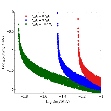
Figure 5: Allowed region in $m_{a}$ - $c_{ll}/f_{a}$ plane, satisfying the muon $(g-2)$ constraint within $2\sigma$ limit for $c_{qq}/f_{a}=8c_{ll}/f_{a}$ (red points), $c_{qq}/f_{a}=9c_{ll}/f_{a}$ (blue points) and $c_{qq}/f_{a}=10c_{ll}/f_{a}$ (green points). Here we have considered one and two loop contributions to $\Delta a_{\mu}$.

In Fig. 4, we show the allowed region in $(c_{ll}/f_{a})-(c_{\gamma\gamma}/f_{a}$) plane from $\Delta a_{\mu}$ observation within $2\sigma$ limit considering both one and two loop contribution. By considering the two loop diagrams, a new parameter $c_{qq}/f_{a}$ appears in our calculation. In this figure we choose $m_{a}=20\rm MeV$ (red points) and $m_{a}=100\rm MeV$ (blue points). With the introduction of the new parameter $c_{qq}/f_{a}$, one can clearly see a certain portion of the allowed region of parameter space is independent of $c_{\gamma\gamma}/f_{a}$. Thus in this region of parameter space, the negative contribution of Fig.1(a) can in principle be offset by the two loop contributions, shown in Fig. 3 independently of $c_{\gamma\gamma}/f_{a}$. In addition, in this region of the parameter space one needs to suppress the effective $c_{\gamma\gamma}/f_{a}$. This is a qualifying criterion for an ALP if it has to explain simultaneously the observed muon $(g-2)$ and the relic density.

Finally in Fig. 5, we show the allowed region of parameter space in $m_{a}$ - $c_{ll}/f_{a}$ plane, considering $c_{\gamma\gamma}/f_{a}=0$ and because of this choice, one can evade all the existing cosmological and astrophysical constraints on the ALP-photon coupling as discussed in [29, 26, 25, 39]. Here we show the allowed regions for muon $(g-2)$, considering $c_{qq}/f_{a}=8c_{ll}/f_{a}$ (red points) , $c_{qq}/f_{a}=9c_{ll}/f_{a}$ (blue points) and $c_{qq}/f_{a}=10c_{ll}/f_{a}$ (green points). Thus one can clearly see from this figure, for $c_{\gamma\gamma}/f_{a}=0$, it is still possible to satisfy the observation of muon $(g-2)$ for $16{\rm MeV}\leq m_{a}\leq 100\rm MeV$ by choosing $c_{qq}/f_{a}$ appropriately. Let us remark that Fig. 1(b) and Fig. 1(c) do not contribute to the calculation of $\Delta a_{\mu}$ because $c_{\gamma\gamma}/f_{a}=0$. As a result, our final conclusion is independent of the choice of $\Lambda$.

IV ALP as a DM candidate

IV.1 Standard Cosmology

In the light of the above discussion, in this section we will discuss the possibility of having ALP as a viable DM candidate. To study the allowed region of our model parameter space from the relic density constraint, we need to solve the Boltzmann equations for the comoving number density of ALP which is defined as $Y_{a}=n_{a}/s(T)$ where $n_{a}$ is the number density of ALP, $s(T)$ is the entropy density of the Universe, and $T$ is the SM bath temperature. In our scenario, the relevant $2\to 2$ number changing processes are $(i)\,aa\to\bar{f}f$, $(ii)\,af(\bar{f})\to\gamma f(\bar{f})$, and $(iii)a\gamma\to\bar{f}f$ where $f=\mu,\tau$. This is to be noted that ALP annihilation into pions are forbidden since in our parameter space of interest $m_{a}<m_{\pi}$.

Considering the above number changing processes, one can write the Boltzmann equation for $Y_{a}$ and it is given as follows.

(a)

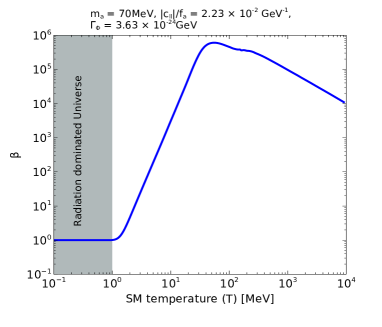
(b)

(c)

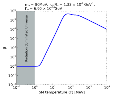
(d)

Figure 6: (a) Evolution of ALP relic density $\Omega_{a}h^{2}$ as a function of SM temperature for $m_{a}=70\rm MeV$ and $|c_{ll}|/f_{a}=2.23\times 10^{-2}{\rm GeV}^{-1}$. Relic density for standard radiation dominated Universe is depicted by red solid line whereas the black solid line depicts the relic abundance of ALP in presence of entropy dilution mechanism for $\Gamma_{\Phi}=3.63\times 10^{-24}{\rm GeV}$. The black dashed line is the equilibrium abundance and the blue solid line represents $\Omega_{a}h^{2}=0.12$. (b) Temperature evolution of $\beta$ for the same parameters as considered in Fig. 6(a). The region below $T=1\rm MeV$ is represented by the grey shaded region. (c) Evolution of ALP relic density for $m_{a}=80\rm MeV$ and $|c_{ll}|/f_{a}=1.33\times 10^{-2}{\rm GeV}^{-1}$. We choose $\Gamma_{\Phi}=6.90\times 10^{-24}{\rm GeV}$ for the entropy dilution mechanism. The color code is same as Fig. 6(a). (d) Temperature evolution of $\beta$ for the same parameter choice as mentioned in Fig. 6(c) and the color code is same as Fig. 6(c). In all the plots we have considered $\rho_{\Phi}^{\rm in}=10^{4}\rho_{\rm rad}(T_{\rm in})$ and $T_{\rm in}=10\rm GeV$.

$$\dfrac{dY_{a}}{dx} = \dfrac{sh_{\rm eff}}{xH}\left[\langle\sigma v\rangle_{aa\to\bar{f}f}({Y_{a}^{\rm eq}}^{2}-Y_{a}^{2})+\Gamma_{f}\left(Y_{a}^{{\rm eq}}-Y_{a}\right)\right]\,\,,$$

where

$$\Gamma_{f} = \sum_{f=\mu,\tau}Y_{f}^{\rm eq}(T)(\langle\sigma v\rangle_{af\to f\gamma}+\langle\sigma v\rangle_{a\bar{f}\to\bar{f}\gamma})$$ (9)

$$+ Y_{\gamma}^{\rm eq}(T)\sum_{f=\mu,\tau}\langle\sigma v\rangle_{a\gamma\to\bar{f}f}.$$

In Eq. LABEL:eq:BE_stancos, $\langle\sigma v\rangle_{aa\to\bar{f}f}$ is the thermally averaged annihilation cross section for $aa\to\bar{f}f$ process, $H$ is the Hubble parameter, $x=m_{a}/T$, and the entropy density $s=2\pi^{2}g_{*s}(T)T^{3}/45$ where $g_{*s}(T)$ is the relativistic degrees of freedom contributing to the entropy density of the Universe. The parameter $h_{\rm eff}$ is defined as

$$h_{\rm eff}=1+\dfrac{1}{3}\dfrac{d\ln g_{*s}(T)}{d\ln T}\,\,.$$ (10)

In Eq. 9, $\langle\sigma v\rangle_{af\to f\gamma}$ ($\langle\sigma v\rangle_{a\bar{f}\to\bar{f}\gamma}$) is the thermally averaged annihilation cross section for $af\to f\gamma$ ($a\bar{f}\to\bar{f}\gamma$) and $\langle\sigma v\rangle_{a\gamma\to\bar{f}f}$ is the thermally averaged annihilation cross section for $a\gamma\to\bar{f}f$.

In Fig. 6(a) and Fig. 6(c), we show the variation of relic density as a function of the SM bath temperature for two benchmark points which are allowed from the muon $(g-2)$ constraint. One can clearly see, for standard radiation dominated Universe, in both the cases, ALP abundance (depicted by red solid lines) exceeds the current bound on DM relic density (depicted by blue solid lines). Thus to get the correct relic density, we need to dilute the final relic abundance. One can dilute the relic density by increasing the parameter $|c_{ll}|/f_{a}$ but in that case we may end up in a region of parameter space where muon $(g-2)$ observation is not satisfied. Another way of diluting the relic is to use the entropy dilution mechanism. Thus to explore both the possibilities, we use the entropy dilution mechanism and vary the amount of dilution (by changing the decay width of the decaying particle) and also the coupling $|c_{ll}|/f_{a}$. The details of the analysis is discussed in the ensuing section.

IV.2 Entropy dilution mechanism

In this section, we will discuss the implication of entropy dilution mechanism on the final relic density of ALP [40, 41, 42, 43]. To study this non-standard cosmological scenario in a model independent way, we have considered a heavy field $\Phi$ which decouples in the early Universe and its total decay width into the SM particles is $\Gamma_{\Phi}$. Since at the time of Big Bang Nucleosynthesis (BBN), our Universe is radiation dominated therefore $\Phi$ must decays before BBN. To get an estimate on the lower limit of decay width of $\Phi$, we use the approximation that the energy density of $\Phi$ is converted into the energy density of radiation ($\rho_{\rm rad}$) instantaneously at or before $T=1\rm MeV$. Using this approximation, the lower limit of $\Gamma_{\Phi}$ is given by

$$\Gamma_{\Phi}\gtrsim 7\times 10^{-25}\rm GeV\,\,.$$ (11)

In order to study the effect of entropy dilution on the final relic of ALP, we need to solve the Boltzmann equations of $X_{\Phi}\equiv\rho_{\Phi}a^{3}$, SM temperature $T$, and comoving number density of ALP ($Y_{a})$ as a function of the scale factor $a$ along with the Hubble parameter $H$ and they are given as follows.

$$\dfrac{dX_{\Phi}}{da} = -\dfrac{\Gamma_{\Phi}X_{\phi}}{aH}\,\,\,,$$ (12)

$$\dfrac{dT}{da} = \dfrac{T}{ah_{\rm eff}}\left[\dfrac{\Gamma_{\Phi}X_{\Phi}}{3a^{3}HsT}-1\right]\,\,\,,$$ (13)

$$\dfrac{dY_{a}}{da} = \dfrac{s}{aH}\left[\langle\sigma v\rangle_{aa\to\bar{f}{f}}\left(Y_{a}^{\rm eq^{2}}-Y_{a}^{2}\right)+\right.$$

$$\left.\Gamma_{f}\left(Y_{a}^{{\rm eq}}-Y_{a}\right)-\dfrac{Y_{a}\Gamma_{\Phi}X_{\Phi}}{a^{3}s^{2}T}\right]\,\,,$$

$$H = \sqrt{\dfrac{8\pi}{3M_{\rm Pl}^{2}}\left(\rho_{\rm rad}+\rho_{\Phi}\right)}\,\,\,,$$ (15)

where $\rho_{\rm rad}=\dfrac{\pi^{2}}{30}g_{*\rho}(T)T^{4}$ and $g_{*\rho}(T)$ is the relativistic degrees of freedom contributing to the energy density of the radiation. $M_{\rm Pl}=1.22\times 10^{19}\rm GeV$ is the Planck mass, and $\Gamma_{f}$ is defined in Eq. 9.

We show the evolution of relic density in presence of the entropy dilution mechanism for the benchmark points considered in Fig. 6 and they are represented by the solid black lines in Fig. 6(a) and Fig. 6(c). In these figures we choose $\Gamma_{\Phi}=3.63\times 10^{-24}\rm GeV$ and $6.90\times 10^{-24}\rm GeV$ for $m_{a}=70\rm MeV$ and $80\rm MeV$ respectively. From the figure one can observe, in presence of the entropy injection to the SM bath after ALP decoupling, we obtain the correct density. However, one needs to ensure that $\Phi$ decays before BBN and our Universe is radiation-dominated during BBN epoch. To check this, we have defined $\beta\equiv 1+{\rho_{\Phi}}/\rho_{\rm rad}$. In order not to jeopardise observed abundances of light nuclei, one requires $\beta\approx 1$ during BBN epoch. In Fig. 6(b), Fig. 6(d) we show the variation of the parameter $\beta$ as a function of SM bath temperature for the same parameter choice as considered in Fig. 6(a) and Fig. 6(c). In the grey shaded region our Universe should be dominated only by the radiation density. In the next section, we will discuss the allowed region of our parameter space from muon $(g-2)$ along with the relic density constraint.

V Other constraints

In this section, we will discuss the constraints on the mass and coupling of ALP with SM fields from various experiments.

• ALP-photon coupling can be constrained from the various astrophysical and cosmological observations. For ALP to be a DM candidate, its lifetime must be greater than $10^{27}s$ as discussed in [29]. However, these constraints are not applicable in our scenario due to the absence of $c_{\gamma\gamma}/f_{a}$.

• The constraints on ALP-photon coupling from LHC [21] arising due to $h\to Za\to l^{+}l^{-}+\gamma\gamma$ and $h\to aa\to 4\gamma$ channels are not considered here since $c_{\gamma\gamma}/f_{a}=0$.

• We have also considered the coupling of ALP to electrons is absent to have ALP to be stable. As a result the constraint on the coupling of ALP with electrons [21] is not applicable in this scenario. However, The coupling of ALP with second and third generation leptons are not suppressed in our scenario and one can constrain ALP-lepton couplings from $h\to Za\to l^{+}l^{-}+\mu^{+}\mu^{-}$, $h\to Za\to l^{+}l^{-}+\tau^{+}\tau^{-}$, $h\to aa\to\mu^{+}\mu^{-}+\mu^{+}\mu^{-}$, $h\to aa\to\tau^{+}\tau^{-}+\mu^{+}\mu^{-}$ as discussed in [21]. However, in the mass range of our interest these processes are kinematically forbidden. The absence of ALP-electron coupling also evades the bound from beam-dump experiment as discussed in [21] .

• The parameter space in $m_{a}$ vs. $|c_{ll}|/f_{a}$ plane can be constrained from the search of light degrees of freedom at BaBar [44]. However in our scenario, the resonant production of $e^{+}e^{-}\to a\mu^{+}\mu^{-}\to\mu^{+}\mu^{-}+\mu^{+}\mu^{-}$ is kinematically forbidden since $m_{a}<2m_{\mu}$.

• In our scenario, the ALP couples with SM quarks and thus this coupling can be constrained from the direct searches. The most stringent bound on the DM-nucleon scattering cross section for sub-GeV DM will arise from CRESST-III [45] and the bound is significant for $m_{a}\gtrsim 100\rm MeV$. We have not considered this bound since we vary the mass of ALP from $1\rm MeV$ to $100\rm MeV$. XENON10T data put significant constraint for $m_{a}\lesssim\rm 100MeV$ if the ALP couples with electron [46]. Recent data from XENON1T [47] experiment put stringent constraint on the ALP mass between $1\rm keV$ to $210\rm keV$ and its coupling with the electron. However in our scenario, the direct search constraints arising from DM-electron scattering are not applicable since ALP coupling with electron is absent.

VI Numerical results for the allowed region from muon $(g-2)$ and relic density constraint

In this section, we show the allowed region of our model parameter space from relic density constraint along with the muon $(g-2)$ satisfied region. To study the ALP relic density, we solve the set of equations given in Eq. 12 - Eq. 15 to calculate the present day comoving number density of ALP ($Y_{a}^{0}$) and the corresponding relic density of ALP is $\Omega_{a}h^{2}=2.755\times 10^{8}(m_{a}/1{\rm GeV})Y_{a}^{0}$. In our numerical analysis, we have considered $T=T_{\rm in}=10{\rm GeV}$, $a=a_{\rm in}=1{\rm GeV}/T_{\rm in}$, and $\rho_{\Phi}=\rho_{\Phi}^{\rm in}=10^{4}\rho_{\rm rad}(T_{\rm in})$ as our initial condition and $\rho_{\rm rad}(T_{\rm in})$ is the radiation density of the Universe at $T_{\rm in}$.

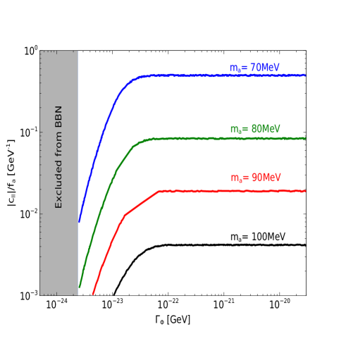
Figure 7: Relic density satisfied (within $2\sigma$ limit) contours in $\Gamma_{\Phi}$ vs. $|c_{ll}|/f_{a}$ plane for ALP masses $100\rm MeV$ (black), $90\rm MeV$ (red), $80\rm MeV$ (green), $70\rm MeV$ (blue). In the grey region, $\Phi$ decay occur after BBN, thus excluded from the observations during the BBN epoch.

In Fig. 7, we show the allowed contours from the relic density constraint within $2\sigma$ limit in $\Gamma_{\Phi}$ and $|c_{ll}|/f_{a}$ plane for four different values of $m_{a}$ such as $100\rm MeV$ (solid black), $90\rm MeV$(solid red), $80\rm MeV$(solid green), $70\rm MeV$ (solid blue). One can clearly see from the figure, for a fixed value of $m_{a}$, there is no variation of $|c_{ll}|/f_{a}$ for the larger values of $\Gamma_{\Phi}$. This is because for large value of $\Gamma_{\Phi}$, the $\Phi$ decays much earlier than the ALP freeze-out and thus at the time of freeze-out there will be no role of $\Gamma_{\Phi}$. However for long lived $\Phi$, the scenario is completely different. In this case, $\Phi$ decay occur during or after ALP freeze-out and thus the decay will dilute the relic significantly. Thus in this regime we need smaller values of $|c_{ll}|/f_{a}$ to satisfy the relic density constraint. The grey region in this figure is excluded from BBN since in this region the Hubble parameter is dominated by the energy density of $\Phi$. As discussed earlier, instantaneous reheating approximation gives the lower limit of $\Gamma_{\Phi}$ to be $7\times 10^{-25}\rm GeV$ however we have numerically checked the lower limit should be $2.5\times 10^{-24}\rm GeV$ and we show the constraint in Fig. 7 considering the lower limit of $\Gamma_{\Phi}$ to be $2.5\times 10^{-24}\rm GeV$.

Finally in Fig. 8, we show the allowed region in $m_{a}$ vs. $|c_{ll}|/f_{a}$ plane from relic density along with the muon $(g-2)$ constraint. In the color bar, we show the variation of the parameter $\kappa$ which is defined as $\kappa=(c_{qq}/f_{a})/(c_{ll}/f_{a})$. From this figure, one can observe that for fixed value of $m_{a}$, we need larger value of $\kappa$ as we decrease $|c_{ll}|/f_{a}$ and this can be understood as follows. The positive contribution to the muon $(g-2)$ arises from the two loop diagrams and it is proportional to $|c_{qq}|/f_{a}=\kappa|c_{ll}|/f_{a}$ and thus the reduction of $|c_{ll}|/f_{a}$ should be counterbalanced by enhancing the value of $\kappa$. In this figure, the blue shaded region is allowed from the relic constraint within $2\sigma$ limit. Here one can observe, for a fixed value of $m_{a}$, one can have multiple values of $|c_{ll}|/f_{a}$ and this is due to the variation of $\Gamma_{\Phi}$ which is varied between $10^{-19}\rm GeV$ to $10^{-24}\rm GeV$. Thus we have found an overlapping region of parameter space between $55{\rm MeV}\lesssim m_{a}\lesssim 100{\rm MeV}$ where ALP can act as a DM and its coupling with muon also ameliorate the tension between theoretical and experimental prediction of muon $(g-2)$.

Figure 8: Allowed region from the muon $(g-2)$ and relic density constraint of ALP in $m_{a}$ vs. $|c_{ll}|/f_{a}$ plane within $2\sigma$ limit. The scattered points are allowed from muon $(g-2)$ constraint and the variation of the quantity $\kappa$ is shown in the color bar. In the blue shaded region, relic density of ALP lies between $0.1176\leq\Omega_{a}h^{2}\leq 0.1224$. In deriving the relic density bound, $\Gamma_{\Phi}$ is varied between $10^{-19}\rm GeV$ to $10^{-24}\rm GeV$.

VII Summary and Conclusions

In this work we have studied the prospect of ALP to be DM candidate along with its muon $(g-2)$ interpretation in a model independent manner. Here we have considered the mass range of ALP to be $1\rm MeV$ to $100\rm MeV$ and its coupling with electron is absent. The coupling of ALP with other charged leptons and SM quarks are flavor universal with coupling co-efficient $c_{ll}/f_{a}$ and $c_{qq}/f_{a}$ respectively. In this set-up we have studied the ALP interpretation of muon $(g-2)$ and DM and our findings are listed below.

• We have considered all possible one and two loop diagrams involving ALP which contribute to the anomalous magnetic moment of muon. We have found that due to the presence of two loop diagrams, in a certain region of parameter space, one can satisfy the muon $(g-2)$ anomaly, even if the coupling of ALP with photon i.e. $c_{\gamma\gamma}/f_{a}$ is absent.

• The above result opens up the possibility of an ALP being a potential DM candidate which can ameliorate the tension between the theoretical prediction and experimental observation of muon $(g-2)$. To ensure the stability of ALP in the cosmological time scale, we require the effective $c_{\gamma\gamma}/f_{a}$ to be tuned to the level of $10^{-22}\rm GeV^{-1}$. As has been stated earlier, we tentatively accept the necessary fine tuning, since its level is still considerably lower than what is required to justify the SM Higgs mass.

• We have calculated the ALP relic density considering all possible $2\to 2$ processes in standard radiation dominated Universe. We have also studied the effect of entropy dilution on the final relic. In our numerical analysis we vary the coupling $c_{ll}/f_{a}$ and also the amount entropy dilution by varying the decay width $\Gamma_{\Phi}$.

• In particular, an ALP in the mass range between $55\rm MeV$ to $100\rm MeV$ can solve the discrepancy between theoretical prediction and experimental observations of muon $(g-2)$ and also serves as a possible DM candidate that saturates the presently estimated relic density.

VIII Acknowledgements

SG would like to acknowledge the financial support in the form of Senior Research Fellowship provided by the University Grants Commission (UGC).

References

- Bennett et al. [2006] G. W. Bennett et al. (Muon g-2), Final Report of the Muon E821 Anomalous Magnetic Moment Measurement at BNL, Phys. Rev. D 73, 072003 (2006), arXiv:hep-ex/0602035 .
- Abi et al. [2021] B. Abi et al. (Muon g-2), Measurement of the Positive Muon Anomalous Magnetic Moment to 0.46 ppm, Phys. Rev. Lett. 126, 141801 (2021), arXiv:2104.03281 [hep-ex] .
- Aoyama et al. [2020] T. Aoyama et al., The anomalous magnetic moment of the muon in the Standard Model, Phys. Rept. 887, 1 (2020), arXiv:2006.04822 [hep-ph] .
- Baek et al. [2001] S. Baek, N. G. Deshpande, X. G. He, and P. Ko, Muon anomalous g-2 and gauged L(muon) - L(tau) models, Phys. Rev. D 64, 055006 (2001), arXiv:hep-ph/0104141 .
- Ma et al. [2002] E. Ma, D. P. Roy, and S. Roy, Gauged L(mu) - L(tau) with large muon anomalous magnetic moment and the bimaximal mixing of neutrinos, Phys. Lett. B 525, 101 (2002), arXiv:hep-ph/0110146 .
- Banerjee et al. [2021] H. Banerjee, B. Dutta, and S. Roy, Supersymmetric gauged model for electron and muon anomaly, JHEP 03, 211, arXiv:2011.05083 [hep-ph] .
- ’t Hooft [1976a] G. ’t Hooft, Symmetry breaking through bell-jackiw anomalies, Phys. Rev. Lett. 37, 8 (1976a).
- ’t Hooft [1976b] G. ’t Hooft, Computation of the quantum effects due to a four-dimensional pseudoparticle, Phys. Rev. D 14, 3432 (1976b).
- Baker et al. [2006] C. A. Baker, D. D. Doyle, P. Geltenbort, K. Green, M. G. D. van der Grinten, P. G. Harris, P. Iaydjiev, S. N. Ivanov, D. J. R. May, J. M. Pendlebury, J. D. Richardson, D. Shiers, and K. F. Smith, Improved experimental limit on the electric dipole moment of the neutron, Phys. Rev. Lett. 97, 131801 (2006).
- Peccei and Quinn [1977a] R. D. Peccei and H. R. Quinn, Constraints Imposed by CP Conservation in the Presence of Instantons, Phys. Rev. D 16, 1791 (1977a).
- Peccei and Quinn [1977b] R. D. Peccei and H. R. Quinn, CP Conservation in the Presence of Instantons, Phys. Rev. Lett. 38, 1440 (1977b).
- Weinberg [1978] S. Weinberg, A new light boson?, Phys. Rev. Lett. 40, 223 (1978).
- Wilczek [1978] F. Wilczek, Problem of strong and invariance in the presence of instantons, Phys. Rev. Lett. 40, 279 (1978).
- Dine and Fischler [1983] M. Dine and W. Fischler, The Not So Harmless Axion, Phys. Lett. B 120, 137 (1983).
- Preskill et al. [1983] J. Preskill, M. B. Wise, and F. Wilczek, Cosmology of the invisible axion, Physics Letters B 120, 127 (1983).
- Abbott and Sikivie [1983] L. Abbott and P. Sikivie, A cosmological bound on the invisible axion, Physics Letters B 120, 133 (1983).
- Marsh [2016] D. J. Marsh, Axion cosmology, Physics Reports 643, 1 (2016), axion cosmology.
- Di Luzio et al. [2020] L. Di Luzio, M. Giannotti, E. Nardi, and L. Visinelli, The landscape of qcd axion models, Physics Reports 870, 1 (2020), the landscape of QCD axion models.
- Arvanitaki et al. [2010] A. Arvanitaki, S. Dimopoulos, S. Dubovsky, N. Kaloper, and J. March-Russell, String Axiverse, Phys. Rev. D 81, 123530 (2010), arXiv:0905.4720 [hep-th] .
- Cicoli et al. [2012] M. Cicoli, M. Goodsell, and A. Ringwald, The type IIB string axiverse and its low-energy phenomenology, JHEP 10, 146, arXiv:1206.0819 [hep-th] .
- Bauer et al. [2017] M. Bauer, M. Neubert, and A. Thamm, Collider Probes of Axion-Like Particles, JHEP 12, 044, arXiv:1708.00443 [hep-ph] .
- Bauer et al. [2020] M. Bauer, M. Neubert, S. Renner, M. Schnubel, and A. Thamm, Axionlike Particles, Lepton-Flavor Violation, and a New Explanation of and , Phys. Rev. Lett. 124, 211803 (2020), arXiv:1908.00008 [hep-ph] .
- Calibbi et al. [2021] L. Calibbi, D. Redigolo, R. Ziegler, and J. Zupan, Looking forward to Lepton-flavor-violating ALPs, JHEP 09, 173, arXiv:2006.04795 [hep-ph] .
- Bauer et al. [2021] M. Bauer, M. Neubert, S. Renner, M. Schnubel, and A. Thamm, Flavor probes of axion-like particles, (2021), arXiv:2110.10698 [hep-ph] .
- Arias et al. [2012] P. Arias, D. Cadamuro, M. Goodsell, J. Jaeckel, J. Redondo, and A. Ringwald, WISPy Cold Dark Matter, JCAP 06, 013, arXiv:1201.5902 [hep-ph] .
- Jaeckel et al. [2014] J. Jaeckel, J. Redondo, and A. Ringwald, 3.55 keV hint for decaying axionlike particle dark matter, Phys. Rev. D 89, 103511 (2014), arXiv:1402.7335 [hep-ph] .
- Ho et al. [2018] S.-Y. Ho, K. Saikawa, and F. Takahashi, Enhanced photon coupling of ALP dark matter adiabatically converted from the QCD axion, JCAP 10, 042, arXiv:1806.09551 [hep-ph] .
- Grossman et al. [2002] Y. Grossman, S. Roy, and J. Zupan, Effects of initial axion production and photon axion oscillation on type Ia supernova dimming, Phys. Lett. B 543, 23 (2002), arXiv:hep-ph/0204216 .
- Cadamuro and Redondo [2012] D. Cadamuro and J. Redondo, Cosmological bounds on pseudo Nambu-Goldstone bosons, JCAP 02, 032, arXiv:1110.2895 [hep-ph] .
- Chang et al. [2018] J. H. Chang, R. Essig, and S. D. McDermott, Supernova 1987A Constraints on Sub-GeV Dark Sectors, Millicharged Particles, the QCD Axion, and an Axion-like Particle, JHEP 09, 051, arXiv:1803.00993 [hep-ph] .
- Chang et al. [2001] D. Chang, W.-F. Chang, C.-H. Chou, and W.-Y. Keung, Large two loop contributions to g-2 from a generic pseudoscalar boson, Phys. Rev. D 63, 091301 (2001), arXiv:hep-ph/0009292 .
- Marciano et al. [2016] W. J. Marciano, A. Masiero, P. Paradisi, and M. Passera, Contributions of axionlike particles to lepton dipole moments, Phys. Rev. D 94, 115033 (2016), arXiv:1607.01022 [hep-ph] .
- Cornella et al. [2020] C. Cornella, P. Paradisi, and O. Sumensari, Hunting for ALPs with Lepton Flavor Violation, JHEP 01, 158, arXiv:1911.06279 [hep-ph] .
- Ge et al. [2021] S.-F. Ge, X.-D. Ma, and P. Pasquini, Probing the dark axion portal with muon anomalous magnetic moment, Eur. Phys. J. C 81, 787 (2021), arXiv:2104.03276 [hep-ph] .
- Buen-Abad et al. [2021] M. A. Buen-Abad, J. Fan, M. Reece, and C. Sun, Challenges for an axion explanation of the muon g 2 measurement, JHEP 09, 101, arXiv:2104.03267 [hep-ph] .
- Leveille [1978] J. P. Leveille, The second-order weak correction to (g - 2) of the muon in arbitrary gauge models, Nuclear Physics B 137, 63 (1978).
- Lindner et al. [2018] M. Lindner, M. Platscher, and F. S. Queiroz, A Call for New Physics : The Muon Anomalous Magnetic Moment and Lepton Flavor Violation, Phys. Rept. 731, 1 (2018), arXiv:1610.06587 [hep-ph] .
- Buttazzo et al. [2021] D. Buttazzo, P. Panci, D. Teresi, and R. Ziegler, Xenon1T excess from electron recoils of non-relativistic Dark Matter, Phys. Lett. B 817, 136310 (2021), arXiv:2011.08919 [hep-ph] .
- Alonso-Álvarez et al. [2020] G. Alonso-Álvarez, R. S. Gupta, J. Jaeckel, and M. Spannowsky, On the Wondrous Stability of ALP Dark Matter, JCAP 03, 052, arXiv:1911.07885 [hep-ph] .
- Scherrer and Turner [1985] R. J. Scherrer and M. S. Turner, Decaying Particles Do Not Heat Up the Universe, Phys. Rev. D 31, 681 (1985).
- Drees and Hajkarim [2018] M. Drees and F. Hajkarim, Dark Matter Production in an Early Matter Dominated Era, JCAP 02, 057, arXiv:1711.05007 [hep-ph] .
- Cosme et al. [2021] C. Cosme, M. a. Dutra, T. Ma, Y. Wu, and L. Yang, Neutrino Portal to FIMP Dark Matter with an Early Matter Era, JHEP 03, 026, arXiv:2003.01723 [hep-ph] .
- Asadi et al. [2021] P. Asadi, T. R. Slatyer, and J. Smirnov, WIMPs Without Weakness: Generalized Mass Window with Entropy Injection, (2021), arXiv:2111.11444 [hep-ph] .
- Lees et al. [2016] J. P. Lees et al. (BaBar), Search for a muonic dark force at BABAR, Phys. Rev. D 94, 011102 (2016), arXiv:1606.03501 [hep-ex] .
- Abdelhameed et al. [2019] A. H. Abdelhameed et al. (CRESST), First results from the CRESST-III low-mass dark matter program, Phys. Rev. D 100, 102002 (2019), arXiv:1904.00498 [astro-ph.CO] .
- Essig et al. [2017] R. Essig, T. Volansky, and T.-T. Yu, New Constraints and Prospects for sub-GeV Dark Matter Scattering off Electrons in Xenon, Phys. Rev. D 96, 043017 (2017), arXiv:1703.00910 [hep-ph] .
- Aprile et al. [2020] E. Aprile et al. (XENON), Excess electronic recoil events in XENON1T, Phys. Rev. D 102, 072004 (2020), arXiv:2006.09721 [hep-ex] .