MST++: Multi-stage Spectral-wise
Transformer for Efficient Spectral Reconstruction

Abstract

Existing leading methods for spectral reconstruction (SR) focus on designing deeper or wider convolutional neural networks (CNNs) to learn the end-to-end mapping from the RGB image to its hyperspectral image (HSI). These CNN-based methods achieve impressive restoration performance while showing limitations in capturing the long-range dependencies and self-similarity prior. To cope with this problem, we propose a novel Transformer-based method, Multi-stage Spectral-wise Transformer (MST++), for efficient spectral reconstruction. In particular, we employ Spectral-wise Multi-head Self-attention (S-MSA) that is based on the HSI spatially sparse while spectrally self-similar nature to compose the basic unit, Spectral-wise Attention Block (SAB). Then SABs build up Single-stage Spectral-wise Transformer (SST) that exploits a U-shaped structure to extract multi-resolution contextual information. Finally, our MST++, cascaded by several SSTs, progressively improves the reconstruction quality from coarse to fine. Comprehensive experiments show that our MST++ significantly outperforms other state-of-the-art methods. In the NTIRE 2022 Spectral Reconstruction Challenge, our approach won the First place. Code and pre-trained models are publicly available at https://github.com/caiyuanhao1998/MST-plus-plus.

1 Introduction

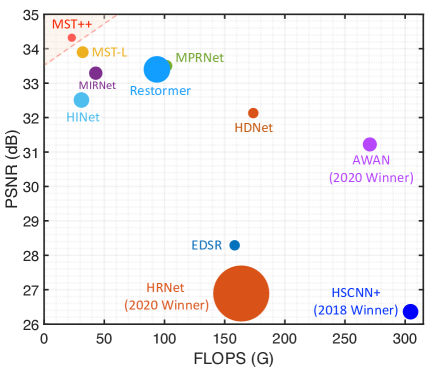
Figure 1: PSNR-Params-FLOPS comparisons with other spectral reconstruction algorithms. The horizontal axis is FLOPS (computational complexity), the vertical axis is PSNR ( performance), and the circle radius is Params (memory cost). Our Multi-stage Spectral-wise Transformer (MST++) surpasses other methods while requiring significantly cheaper FLOPS and Params.

Hyperspectral imaging records the real-world scene spectra in narrow bands, where each band captures the information at a specific spectral wavelength. Compared to normal RGB images, HSIs have more spectral bands to store richer information and delineate more details of the captured scenes. Because of this advantage, HSIs have wide applications such as medical image processing [8, 51, 57], remote sensing [10, 54, 82], object tracking [35, 61], and so on. Nonetheless, such HSIs with plentiful spectral information is time-consuming that spectrometers are used to scan the scenes along the spatial or spectral dimension. This limitation impedes the application scope of HSIs, especially in dynamic or real-time scenes.

One way to solve this problem is to develop snapshot compressive imaging (SCI) systems and computational reconstruction algorithms [13, 12, 29, 47, 80, 55, 56, 59, 33, 73, 74, 48, 9, 58, 52] from 2D measurement to 3D HSI cube. Nevertheless, these methods rely on expensive hardware devices. To reduce costs, spectral reconstruction (SR) algorithms are proposed to reconstruct the HSI from a given RGB image, which can be easily obtained by RGB cameras.

Conventional SR methods are mainly based on sparse coding or relatively shallow learning models. Nonetheless, these model-based methods suffer from limited representing capacity and poor generalization ability. Recently, with the development of deep learning, SR has witnessed significant progress. Deep convolutional neural networks (CNNs) have been applied to learn the end-to-end mapping function from RGB images to HSI cubes. Although impressive performance have been achieved, these CNN-based methods show limitations in capturing long-range dependencies and inter-spectra self-similarity.

In recent years, the natural language processing (NLP) model, Transformer [70], has been applied in computer vision and achieved great success. The multi-head self-attention (MSA) mechanism in Transformer does better in modeling long-range dependencies and non-local self-similarity than CNN, which can alleviate the limitations of CNN-based SR algorithms. However, directly using standard Transformer [25, 49] for SR will encounter two main issues. (i) Global [25] and local [49] Transformer captures inter-actions of spatial regions. Yet, the HSI representations are spatially sparse while spectrally highly self-similar. Thus, modeling spatial inter-dependencies may-be less cost-effective than capturing inter-spectra correlations. (ii) On the one hand, the computational complexity of standard global MSA is quadratic to the spatial dimension, which is a huge burden that may be unaffordable. On the other hand, local window-based MSA suffers from limited receptive fields within position-specific windows.

To address the aforementioned limitations, we propose the first Transformer-based framework, Multi-stage Spectral-wise Transformer (MST++) for efficient spectral reconstruction from RGB images. Notely, our MST++ is based on the prior work MST [13], which is customized for spectral compressive imaging restoration. Firstly, we note that HSI signals are spatially sparse while spectrally self-similar. Based on this nature, we adopt the Spectral-wise Multi-head Self-Attention (S-MSA) to compose the basic unit, Spectral-wise Attention Block (SAB). S-MSA treats each spectral feature map as a token to calculate the self-attention along the spectral dimension. Secondly, our SABs build up our proposed Single-stage Spectral-wise Transformer (SST) that exploits a U-shaped structure to extract multi-resolution spectral contextural information which is critical for HSI restoration. Finally, our MST++, cascaded by several SSTs, develops a multi-stage learning scheme to progressively improve the reconstruction quality from coarse to fine, which significantly boosts the performance.

The main contributions of this work are listed as follow.

• We propose a novel framework, MST++, for SR. To the best of our knowledge, it is the first attempt to explore the potential of Transformer in this task.

• We validate a series of natural image restoration models on this SR task. Toward them, we propose a Top-K multi-model ensemble strategy to improve the SR performance. Codes and pre-trained models of these methods are made publicly available to serve as a baseline and toolbox for further research in this topic.

• Quantitative and qualitative experiments demonstrate that our MST++ dramatically outperforms SOTA methods while requiring much cheaper Params and FLOPS. Surprisingly, our MST++ won the First place in NTIRE 2022 Spectral Reconstruction Challenge [5].

2 Related Work

2.1 Hyperspectral Image Aquisition

Traditional imaging systems for collecting HSIs often adopt spectrometers to scan the scene along the spatial or spectral dimensions. Three main types of scanners including whiskbroom scanner, pushroom scanner, and band sequential scanner are often used to capture HSIs. These scanners have been widely used in detecting, remote sensing, medical imaging, and environmental monitoring for decades. For example, pushbroom scanner and whiskbroom scanner have been used in satellite sensors [11, 64] for photogrammetric and remote sensing. However, the scanning procedure usually requires a long time, which makes it unsuitable for measuring dynamic scenes. Besides, the imaging devices are usually too large physically to be plugged in portable platforms. To address these limitations, researchers have developed SCI systems [50, 71, 72, 18, 26] to capture HSIs, where the 3D HSI cube is compressed into a single 2D measurement [81]. Among these SCI systems, coded aperture snapshot spectral imaging (CASSI) [56, 71] stands out and forms one promising research direction. Nonetheless, the SCI systems remain prohibitively expensive to date for consumer grade use. Even ”low-cost” SCI systems are often in the $ 10K - $ 100K. Therefore, the SR topic has significant research and practical value.

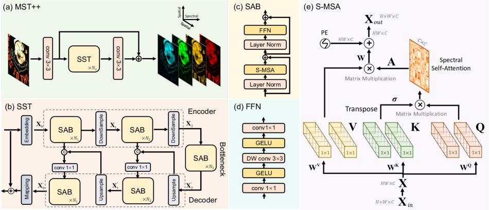
Figure 2: The overall pipeline of the proposed solution MST++. (a) Multi-stage Spectral-wise Transformer. (b) Single-stage Spectral-wise Transformer. (c) Spectral-wise Attention Block. (d) Feed Forward Network. (e) Spectral-wise Multi-head Self-Attention.

2.2 Spectral Reconstruction from RGB

Conventional SR methods [1, 2, 34, 66, 62] are mainly based on hand-crafted hyperspectral priors. For instance, Paramar et al. [62] propose a data sparsity expending method for HSI reconstruction. Arad et al. [2] propose a sparse coding method that create a dictionary of HSI signals and their RGB projections. Aeschbacher et al. [1] suggest using relatively shallow learning models from a specific spectral prior to fulfill spectral super-resolution. However, these model-based methods suffer from limited representing capacities and poor generalization ability.

Recently, inspired by the great success of deep learning in natural image restoration [92, 24, 46, 12, 40, 38, 39, 63, 30, 31], CNNs have been exploited to learn the underlying mapping function from RGB to HSI [78, 67, 87, 68, 28]. For instance, Xiong et al. [78] propose a unified HSCNN framework for HSI reconstruction from both RGB images and compressive measurements. Shi et al. [67] use adapted residual blocks to build up a deep residual network HSCNN-R for SR. Zhang et al. [87] customize a pixel-aware deep function-mixture network consisting to model the RGB-to-HSI mapping. However, these CNN-based SR methods achieve impressive results but show limitations in capturing non-local self-similarity and long-range inter-dependencies.

2.3 Vision Transformer

The NLP model Transformer [70] is proposed for machine translation. In recent years, it has been introduced into computer vision and gained much popularity due to its advantage in capturing long-range correlations between spatial regions. In high-level vision, Transformer has been widely applied in image classification [49, 7, 25, 27, 65, 19], object detection [93, 86, 22, 23, 60, 6], semantic segmentation [76, 16, 90, 91, 77, 69], human pose estimation [43, 79, 14, 15, 32, 37, 89, 42, 53], etc. In addition, vision Transformer has also been used in low-level vision [13, 17, 20, 24, 44, 46, 47]. For instance, Cai et al. [13] propose the first Transformer-based end-to-end framework MST for HSI reconstruction from compressive measurements. Lin et al. [47] embed the HSI sparsity into Transformer to establish a coarse-to-fine learning scheme for spectral comrpessive imaging. The prior work Uformer [75] adopts a U-shaped structure built up by Swin Transformer [49] blocks for natural image restoration. Nonetheless, to the best of our knowledge, the potential of Transformer in spectral super-resolution has not been explored. This work aims to fill this research gap.

3 Method

3.1 Network Architecture

As shown in Fig. 2, (a) depicts the proposed Multi-stage Spectral-wise Transformer (MST++), which is cascaded by $N_{s}$ Single-stage Spectral-wise Transformers (SSTs). Our MST++ takes a RGB image as the input and reconstructs its HSI counterpart. A long identity mapping is exploited to ease the training procedure. Fig. 2 (b) shows the U-shaped SST consisting of an encoder, a bottleneck, and a decoder. The embedding and mapping block are single $conv$3$\times$3 layers. The feature maps in the encoder sequentially undergo a downsampling operation (a strided $conv$4$\times$4 layer), $N_{1}$ Spectral-wise Attention Blocks (SABs), a downsampling operation, and $N_{2}$ SABs. The bottleneck is composed of $N_{3}$ SABs. The decoder employs a symmetrical architecture. The upsampling operation is a strided deconv2$\times$2 layer. To avoid the information loss in the downsampling, skip connections are used between the encoder and decoder. Fig. 2 (c) illustrates the components of SAB, i.e., a Feed Forward Network (FFN as shown in Fig. 2 (d) ), a Spectral-wise Multi-head Self-Attention (S-MSA), and two layer normalization. Details of S-MSA are given in Fig. 2 (e).

3.2 Spectral-wise Multi-head Self-Attention

Suppose $\mathbf{X}_{in}\in\mathbb{R}^{H\times W\times C}$ as the input of S-MSA, which is reshaped into tokens $\mathbf{X}\in\mathbb{R}^{HW\times C}$. Then $\mathbf{X}$ is linearly projected into query $\mathbf{Q}\in\mathbb{R}^{HW\times C}$, key $\mathbf{K}\in\mathbb{R}^{HW\times C}$, and value $\mathbf{V}\in\mathbb{R}^{HW\times C}$:

$$\mathbf{Q}=\mathbf{X}\mathbf{W}^{\mathbf{Q}},\mathbf{K}=\mathbf{X}\mathbf{W}^{\mathbf{K}},\mathbf{V}=\mathbf{X}\mathbf{W}^{\mathbf{V}},\vspace{0.2mm}$$ (1)

where $\mathbf{W}^{\mathbf{Q}}$, $\mathbf{W}^{\mathbf{K}}$, and $\mathbf{W}^{\mathbf{V}}\in\mathbb{R}^{C\times C}$ are learnable parameters; $biases$ are omitted for simplification. Subsequently, we respectively split $\mathbf{Q}$, $\mathbf{K}$, and $\mathbf{V}$ into $N$ heads along the spectral channel dimension: $\mathbf{Q}=[\mathbf{Q}_{1},\ldots,\mathbf{Q}_{N}]$, $\mathbf{K}=[\mathbf{K}_{1},\ldots,\mathbf{K}_{N}]$, and $\mathbf{V}=[\mathbf{V}_{1},\ldots,\mathbf{V}_{N}]$. The dimension of each head is $d_{h}=\frac{C}{N}$. Please note that Fig. 2 (e) depicts the situation with $N$ = 1 and some details are omitted for simplification. Different from original MSAs, our S-MSA treats each spectral representation as a token and calculates self-attention for $head_{j}$:

$$\mathbf{A}_{j}=\text{softmax}(\sigma_{j}\mathbf{K}_{j}^{\text{T}}\mathbf{Q}_{j}),~{}~{}{head}_{j}=\mathbf{V}_{j}\mathbf{A}_{j},\vspace{-0.2mm}$$ (2)

where $\mathbf{K}_{j}^{\text{T}}$ denotes the transposed matrix of $\mathbf{K}_{j}$. Because the spectral density varies significantly with respect to the wavelengths, we use a learnable parameter $\sigma_{j}\in\mathbb{R}^{1}$ to adapt the self-attention $\mathbf{A}_{j}$ by re-weighting the matrix multiplication $\mathbf{K}_{j}^{\text{T}}\mathbf{Q}_{j}$ inside $head_{j}$. Subsequently, the outputs of $N$ heads are concatenated to undergo a linear projection and then is added with a position embedding:

$$\text{S-MSA}(\mathbf{X})=\big{(}\mathop{\text{Concat}}\limits_{j=1}^{N}(head_{j})\big{)}\mathbf{W}+f_{p}(\mathbf{V}),$$ (3)

where $\mathbf{W}\in\mathbb{R}^{C\times C}$ are learnable parameters, $f_{p}(\cdot)$ is the function to generate position embedding. It consists of two depth-wise conv3$\times$3 layers, a GELU activation, and reshape operations. The HSIs are sorted by the wavelength along the spectral dimension. Therefore, we exploit this embedding to encode the position information of different spectral channels. Finally, we reshape the result of Eq. (3) to obtain the output feature maps $\mathbf{X}_{out}\in\mathbb{R}^{H\times W\times C}$.

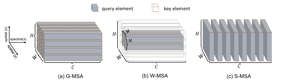
Figure 3: Diagram of different MSAs. The dark colored box represents $query$ element and the dashed box denotes $key$ element. (a) Global MSA samples all the tokens (pixel vectors) as $query$ and $key$ elements. (b) W-MSA calculates the self-attention inside position-specific windows. (c) The adopted S-MSA treats each spectral channel as a token and calculates the self-attention along the spectral dimension.

3.3 Discussion with Original Transformers

In this section, we introduce the general paradigm of MSA in Transformer and then we analyze the computational complexity of the spatial-wise MSAs in original Transformers and the adopted S-MSA.

3.3.1 General Paradigm of MSA

We denote the input token as $\mathbf{X}\in\mathbb{R}^{n\times C}$, where $n$ is to be determined. In spatial-wise MSAs, $n$ denotes the number of tokens. In S-MSA, $n$ represents the dimension of the token. $\mathbf{X}$ is firstly linearly projected into query $\mathbf{Q}\in\mathbb{R}^{n\times C}$, key $\mathbf{K}\in\mathbb{R}^{n\times C}$, and value $\mathbf{V}\in\mathbb{R}^{n\times C}$:

$$\mathbf{Q}=\mathbf{X}\mathbf{W^{Q}},\mathbf{K}=\mathbf{X}\mathbf{W^{K}},\mathbf{V}=\mathbf{X}\mathbf{W^{V}},$$ (4)

where $\mathbf{W^{Q}},\mathbf{W^{K}}$, and $\mathbf{W^{V}}\in\mathbb{R}^{C\times C}$ are learnable parameters; biases are omitted for simplification. Subsequently, we respectively split $\mathbf{Q}$, $\mathbf{K}$, and $\mathbf{V}$ into $N$ heads along the spectral channel dimension: $\mathbf{Q}=[\mathbf{Q}_{1},\ldots,\mathbf{Q}_{N}]$, $\mathbf{K}=[\mathbf{K}_{1},\ldots,\mathbf{K}_{N}]$, and $\mathbf{V}=[\mathbf{V}_{1},\ldots,\mathbf{V}_{N}]$. The dimension of each head is $d_{h}=\frac{C}{N}$. Then MSA calculates the self-attention for each $head_{j}$:

$$head_{j}=\text{MSA}(\mathbf{Q}_{j},\mathbf{K}_{j},\mathbf{V}_{j}).$$ (5)

Subsequently, the outputs of $N$ heads are concatenated along the spectral dimension and undergo a linear projection to generate the output feature map $\textbf{X}_{out}\in\mathbb{R}^{n\times C}$:

$$\textbf{X}_{out}=\big{(}\mathop{\text{Concat}}\limits_{j=1}^{N}(head_{j})\big{)}\mathbf{W},$$ (6)

where $\mathbf{W}\in\mathbb{R}^{C\times C}$ are learnable parameters. Please note that some other contents such as the position embedding are omitted for simplification. Because we only compare the main difference between original spatial-wise MSAs and S-MSA, i.e., the specific formulation of Eq. (5).

MSA Scheme	Global MSA	Local W-MSA	S-MSA
Receptive Field	Global	Local	Global
Complexity to $HW$	Quadratic	Linear	Linear
Calculating Wise	Spatial	Spatial	Spectral

Table 1: Comparisons of the properties of different MSAs.

3.3.2 Spatial-wise MSA

The spatial-wise MSA treats a pixel vector along the spectral dimension as a token and then calculates the self-attention for each $head_{j}$. Thus, Eq. (5) can be specified as

$$head_{j}=\mathbf{A}_{j}\mathbf{V}_{j},~{}~{}\mathbf{A}_{j}=\text{softmax}(\frac{\mathbf{Q}_{j}\mathbf{K}_{j}^{T}}{\sqrt{d_{h}}}).$$ (7)

Eq. (7) neads to be calculated for $N$ times. Therefore, the computational complexity of spatial-wise MSA is

$$O(\text{Spatial-MSA})=N(n^{2}d_{h}+n^{2}d_{h})=2n^{2}C.$$ (8)

The spatial-wise MSA is mainly divided into two categories: global MSA [25] and local window-based MSA [49]. Now we analyze these two kinds of MSAs.

Global MSA. As shown in Fig. 3 (a), global MSA samples all the tokens as $key$ and $query$ elements, and then calculates the self-attention. Thus, the number of tokens $n$ ($key$ or $query$ elements) is equal to $HW$. Then, according to Eq. (8), the computational complexity of global MSA is

$$O(\text{Global MSA})=2(HW)^{2}C,$$ (9)

which is quadratic to the spatial size of the input feature map. Global MSA enjoys a very large receptive field but its computational cost is nontrivial and sometimes unaffordable. Meanwhile, sampling redundant $key$ elements may easily lead to over-smooth results [41] and even non-convergence issue [93]. To cut down the computational cost, researchers propose local window-based MSA.

Window-based MSA. As depicted in Fig. 3 (b), W-MSA firstly splits the feature map into non-overlapping windows at size of $M^{2}$ and samples all the tokens inside each window to calculate self-attention. Hence, the number of tokens $n$ is equal to $M^{2}$ and W-MSA is conducted $\frac{HW}{M^{2}}$ times for all windows. Thus, the computational complexity is

$$O(\text{W-MSA})=\frac{HW}{M^{2}}(2(M^{2})^{2}C)=2M^{2}HWC,$$ (10)

which is linear to the spatial size ($HW$). W-MSA enjoys low computational cost but suffers from limited receptive fields inside position-specific windows. As a result, some highly related non-local tokens may be neglected.

Original spatial-wise MSAs aim to capture the long-range dependencies of spatial regions. However, the HSI representations are spatially sparse while spectrally similar and correlated. Capturing spatial-wise interactions may be less cost-effective than modeling the spectral-wise correlations. Based on this HSI characteristic, we adopt S-MSA.

3.3.3 S-MSA

As shown in Fig. 3 (b), S-MSA treats each spectral feature map as a token and calculates the self-attention along the spectral dimension. Then Eq. (5) is specified as

$$\mathbf{A}_{j}=\text{softmax}(\sigma_{j}\mathbf{K}_{j}^{\text{T}}\mathbf{Q}_{j}),~{}~{}{head}_{j}=\mathbf{V}_{j}\mathbf{A}_{j},$$ (11)

where $\mathbf{K}_{j}^{\text{T}}$ denotes the transposed matrix of $\mathbf{K}_{j}$. We note that the spectral density varies significantly with respect to the wavelengths. Therefore, we exploit a learnable parameter $\sigma_{j}\in\mathbb{R}^{1}$ to adapt the self-attention $\mathbf{A}_{j}$ by re-weighting the matrix multiplication $\mathbf{K}_{j}^{\text{T}}\mathbf{Q}_{j}$ inside $head_{j}$. Because S-MSA treats a whole feature map as a token, the dimension of each token $n$ is equal to $HW$. Eq. (11) needs to be calculated $N$ times. Thus, the complexity of S-MSA is

$$O(\text{S-MSA})=N(d_{h}^{2}n+d_{h}^{2}n)=\frac{2HWC^{2}}{N}.$$ (12)

The computational complexity of W-MSA and S-MSA are linear to the spatial size ($HW$), which is much cheaper than that of global MSA (quadratic to $HW$). Nonetheless, S-MSA treats each spectral feature as a token. When calculating the self-attention $\mathbf{A}_{j}$, S-MSA views the global representations and $\mathbf{A}_{j}$ functions as global spatial positions. Therefore, the receptive fields of S-MSA are global and not limited to the position-specific windows.

In addition, S-MSA calculates self-attention along the spectral dimension, which is based on HSI characteristics and more suitable for HSI reconstruction when compared to spatial-wise MSAs. Thus, S-MSA is considered to be more cost-effective than global MSA and W-MSA.

For brevity, we summarize the properties of global MSA, window-based MSA, and S-MSA in Tab. 1. S-MSA enjoys global receptive fields, models the spectral-wise self-similarity, and requires linear computational costs.

3.4 Ensemble Strategy

In NTIRE 2022 Spectral Reconstruction Challenge, we adopt three ensemble strategies including self-ensemble, multi-scale ensemble, and Top-K multi-model ensemble to improve the performance and generality of our MST++. Now in this part, we describe them in details.

3.4.1 Self-Ensemble

The RGB input is flipped up/down/left/right or rotated 90°/180°/270° to be fed into the network. Subsequently, the outputs are transformed to the original state to be averaged.

3.4.2 Multi-scale Ensemble

We respectively train our models with patches at size of 256$\times$256, 128$\times$128, and 64$\times$64. Then the outputs (whole images) are averaged to improve the restoration quality.

3.4.3 Top-K Multi-model Ensemble

We also train MIRNet [84], MPRNet [85], Restormer [83], HINet [21], and MST [13] families. The Top-K performers are selected for SR. Then we conduct our Top-K multi-model ensemble to fuse these reconstructed HSIs as

$$\mathbf{Y}_{ens}=\sum_{i=1}^{\text{K}}\alpha_{i}\mathbf{\hat{Y}}^{t}_{i},$$ (13)

where $\mathbf{Y}_{ens}\in\mathbb{R}^{H\times W\times N_{\lambda}}$ denotes the ensembled HSIs, $\mathbf{\hat{Y}}^{t}_{i}$ represents the reconstructed HSIs of the $i$-th model, and $\alpha_{i}$ represents hyperparameter satisfying $\sum_{i=1}^{\text{K}}\alpha_{i}=1$.

4 Experiment

4.1 Dataset

The dataset provided by NTIRE 2022 Spectral Reconstruction Challenge contains 1000 RGB-HSI pairs. This dataset is split into train, valid, and test subsets in proportional to 18:1:1. Each HSI at size of 482$\times$512 has 31 wavelengths from 400 nm to 700 nm. To generate the corresponding RGB counterpart $\mathbf{I}\in\mathbb{R}^{H\times W\times 3}$, a transformation matrix $\mathbf{M}\in\mathbb{R}^{N_{\lambda}\times 3}$ is applied to the ground-truth HSI cube $\mathbf{Y}\in\mathbb{R}^{H\times W\times N_{\lambda}}$ as

$$\mathbf{I}=\mathbf{Y}\times\mathbf{M}.$$ (14)

Then the generated RGB images are injected with shot noise to simulate the real-camera situation.

4.2 Implementation Details

During the training procedure, RGB images are linearly rescaled to [0, 1], after which $128\times 128$ RGB and HSI sample pairs are cropped from the dataset. The batch size is set to 20 and the parameter optimization algorithm chooses Adam modification with $\beta_{1}=0.9$ and $\beta_{2}=0.999$. The learning rate is initialized as 0.0004 and the Cosine Annealing scheme is adopted for 300 epochs. The training data is augmented with random rotation and flipping. The proposed MST++ has been implemented on the Pytorch framework and approximately 48 hours are required for training a network on a single RTX 3090 GPU. MRAE loss function between the predicted and ground-truth HSI is adopted as the objective. In the implementation of our MST++, we set $N_{s}$ = 3, $N_{1}$ = $N_{2}$ = $N_{3}$ = 1, $C$ = 31.

During the testing phase, the RGB image is also linearly rescaled to [0, 1] and fed into the network to fulfill the spectral recovery. Our MST++ takes 102.48 ms for per image (size 482$\times$512$\times$3) reconstruction on an RTX 3090 GPU.

We adopt three evaluation metrics to assess the model performance. The first metric is mean relative absolute error (MRAE) that computes the pixel-wise disparity between all wavelengths of the reconstructed and ground-truth HSIs. MRAE can be formulated as

$$\text{MRAE}(\mathbf{Y},\mathbf{\hat{Y}})=\frac{1}{N}\sum_{i=1}^{N}\frac{\big{|}~{}\mathbf{Y}[i]-\mathbf{\hat{Y}}[i]~{}\big{|}}{\mathbf{Y}[i]},$$ (15)

where $\mathbf{\hat{Y}}\in\mathbb{R}^{H\times W\times N_{\lambda}}$ indicates the reconstructed HSI cube and $N=H\times W\times N_{\lambda}$ denotes the number of all values on the image. The second metric is the root mean square error (RMSE) that is defined as

$$\text{RMSE}(\mathbf{Y},\mathbf{\hat{Y}})=\sqrt{\frac{1}{N}\sum_{i=1}^{N}\big{(}\mathbf{Y}[i]-\mathbf{\hat{Y}}[i]\big{)}^{2}}.$$ (16)

Since the deciding metric for the NTIRE 2022 Spectral Reconstruction Challenge is MRAE, we directly set it as the training objective for our SR models. The last metric is the Peak Signal-to-Noise Ratio (PSNR).

NTIRE 2022 HSI Dataset - Valid						NTIRE 2022 HSI Dataset - Test
Method	Params (M)	FLOPS (G)	MRAE	RMSE	PSNR	Username	MRAE	RMSE
HSCNN+ [67]	4.65	304.45	0.3814	0.0588	26.36	pipixia	0.2434	0.0411
HRNet [88]	31.70	163.81	0.3476	0.0550	26.89	uslab	0.2377	0.0391
EDSR [45]	2.42	158.32	0.3277	0.0437	28.29	orange_dog	0.2377	0.0376
AWAN [36]	4.04	270.61	0.2500	0.0367	31.22	askldklasfj	0.2345	0.0361
HDNet [29]	2.66	173.81	0.2048	0.0317	32.13	HSHAJii	0.2308	0.0364
HINet [21]	5.21	31.04	0.2032	0.0303	32.51	ptdoge_hot	0.2107	0.0365
MIRNet [84]	3.75	42.95	0.1890	0.0274	33.29	test_pseudo	0.2036	0.0324
Restormer [83]	15.11	93.77	0.1833	0.0274	33.40	gkdgkd	0.1935	0.0322
MPRNet [85]	3.62	101.59	0.1817	0.0270	33.50	deeppf	0.1767	0.0322
MST-L [13]	2.45	32.07	0.1772	0.0256	33.90	mialgo_ls	0.1247	0.0257
MST++	1.62	23.05	0.1645	0.0248	34.32	MST++*	0.1131	0.0231

Table 2: Comparisons with SOTA methods on NTIRE 2022 HSI datasets (valid and test). * represents using ensembled models.

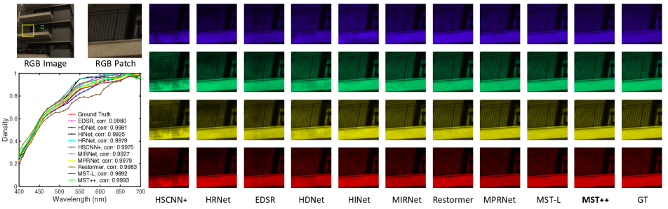
Figure 4: Reconstructed HSI comparisons of Scene ARAD_1K_0922 with 4 out of 31 spectral channels. 9 SOTA algorithms and our MST++ are included. The spectral curves (bottom-left) are corresponding to the selected green box of the RGB image. Please zoom in.

Method	Baseline	SW-MSA	W-MSA	G-MSA	S-MSA
MRAE	0.3177	0.2839	0.2624	0.1821	0.1645
RMSE	0.0453	0.0399	0.0375	0.0271	0.0248
Params (M)	1.30	1.60	1.60	1.60	1.62
FLOPS (G)	17.68	24.10	24.10	25.11	23.05

(a)

$N_{s}$	1	2	3	4
MRAE	0.1761	0.1716	0.1645	0.1711
RMSE	0.0266	0.0269	0.0248	0.0265
Params (M)	0.55	1.08	1.62	2.16
FLOPS (G)	8.10	15.57	23.05	30.52

(b)

Table 3: Ablations. We train models on the train set and test on the valid set. MRAE, RMSE, Params, and FLOPS are reported.

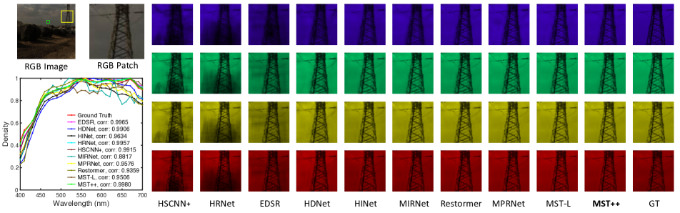
Figure 5: Reconstructed HSI comparisons of Scene ARAD_1K_0924 with 4 out of 31 spectral channels. 9 SOTA algorithms and our MST++ are included. The spectral curves (bottom-left) are corresponding to the selected green box of the RGB image. Please zoom in.

4.3 Main Results

4.3.1 Quantitative Results on Valid Set

We compare our MST++ with SOTA methods including two SCI reconstruction methods (MST [13] and HDNet [29]), three SR algorithms (HSCNN+ [67], AWAN [36] and HRNet [88]), and five natural image restoration models (MIRNet [84], MPRNet [85], Restormer [83], HINet [21], EDSR [45]) on the valid set. Please note that HSCNN+ [67], AWAN [36] and HRNet [88] are the winners of NTIRE 2018 [3] and 2020 [4] Spectral Reconstruction Challenges. The results are listed in Tab. 2. Our MST++ significantly outperforms SOTA methods by a large margin while requiring the least Params and FLOPS. For instance, our MST++ achieves 3.10, 7.43, and 7.96 dB improvement in PSNR while only requiring 40.10% (1.62 / 4.04), 5.11%, 34.84% Params and 8.52% (23.05 / 270.61), 14.07%, 7.57% FLOPS when compared to AWAN, HRNet, and HSCNN+.

To intuitively show the superiority of MST++, we provide PSNR-Params-FLOPS comparisons of different algorithms in Fig. 1. The vertical axis is PSNR (performance), the horizontal axis is FLOPS (computational cost), and the circle radius is Params (memory cost). It can be seen that our MST++ takes up the top-left corner, exhibiting the extreme efficiency advantages of our method.

4.3.2 Quantitative Results on Test Set

Tab. 2 lists the top-12 leaders of NTIRE 2022 Spectral Challenge (test set), where * indicates using ensembled models. Impressively, our method won the championship out of 231 participants, suggesting the superiority of our MST++.

4.3.3 Qualitative Results

Fig. 4 and 5 compares the reconstructed HSIs with 4 out of 31 spectral channels of nine SOTA methods and our MST++ on the valid set. Please zoom in for a better view. The top-left part depicts the input RGB image. The right part shows the reconstructed HSI patches of the selected yellow boxes in RGB image. It can be observed that previous methods show limitations in HSI detail restoration. They either achieve over-smooth HSIs sacrificing fine-grained contents and structural details, or introduce unpleasing artifacts and blotchy textures. By contrast, MST++ does better in producing perceptually-pleasing and sharp-edge HSIs, and preserving the spatial smoothness of the homogeneous regions. This is mainly because our MST++ excels at modeling inter-spectra self-similarity and dependencies. Besides, the bottom-left part exhibits the spectral density curves corresponding to the picked region of the green box in the RGB image. The highest correlation and coincidence between our curve and the ground truth verify the spectral-wise consistency restoration effectiveness of MST++.

4.4 Ablation Study

we use the valid subset to conduct ablations. The baseline model is derived by removing S-MSA from MST++.

4.4.1 Self-Attention Mechanism

We have discussed different self-attention mechanisms in Sec. 3.3. In this part, we conduct ablation studies to verify the performance of these MSAs including global MSA (G-MSA) [25], local window-based MSA (W-MSA) [49], Swin MSA (SW-MSA) [49], and the adopted S-MSA [13]. The results are reported in Tab. LABEL:tab:attention. For fairness, the Params of models using different MSAs are set to the same value. Notely, the input feature of G-MSA is downscaled into $\frac{1}{4}$ size to avoid out of memory. It can be observed that our adopted S-MSA achieves the most significant improvement while requiring the least memory and computational costs. To be specific, when we respectively apply SW-MSA, W-MSA, G-MSA, and S-MSA, the performance is improved by 0.0338, 0.0553, 0.1356, and 0.1532 in MRAE while increasing 6.42, 6.42, 7.43, and 5.37 GFLOPS. As analyzed in Sec. 3.3, these results mainly stem from the HSI spatially sparse while spectrally self-similar nature. Thus, capturing inter-spectra dependencies is more cost-effective than modeling correlations of spatial regions.

4.4.2 Stage Number

We change the stage number $N_{s}$ of MST++ to investigate its effect. The results are shown in Tab. LABEL:tab:stage. When $N_{s}$ = 3, the performance achieves its peak. Therefore, we finally adopt 3-stage MST++ as our SR model.

4.4.3 Ensemble Strategy

In Sec. 3.4, we adopt three ensemble strategies for NTIRE 2022 Spectral Reconstruction Challenge. In this part, we perform ablations to study their effects. On the valid set, self-ensemble, multi-scale ensemble, and Top-K (K is set to 5) multi-model ensemble respectively achieve improvements by 0.015, 0.033, and 0.045 in terms of MRAE.

5 Future Work

Until now, there has not been a low-cost high-accuracy open-source baseline for SR research. Our MST++ aims to fill this gap. Moreover, all the source code and pre-trained models in Tab. 2 (valid) including 11 SOTA methods are made publicly available. Our goal is to provide a model zoo and toolbox to benefit the community.

6 Conclusion

In this paper, we propose the first Transformer-based framework, MST++, for spectral reconstruction from RGB. Based on the HSI spatially sparse while spectrally self-similar nature, we adopt S-MSA that treats each spectral feature map as a token for self-attention calculation to compose the basic unit SAB. Then SABs build up SST. Eventually, our MST++ is cascaded by several SSTs. Enjoying a multi-stage learning scheme, MST++ progressively improves the reconstruction quality from coarse to fine. Quantitative and qualitative experiments demonstrate that our MST++ dramatically surpasses SOTA methods while requiring cheaper memory and computational costs. Impressively, our MST++ won the First place in the NTIRE 2022 Challenge on Spectral Reconstruction from RGB.

Acknowledgements: This work is partially supported by the NSFC fund (61831014), the Shenzhen Science and Technology Project under Grant (ZDYBH201900000002, CJGJZD20200617102601004), the Westlake Foundation (2021B1501-2). Zudi Lin and Hanspeter Pfister acknowledge the support from NSF award IIS-2124179 and Google Cloud research credits.

References

- [1] Jonas Aeschbacher, Jiqing Wu, and Radu Timofte. In defense of shallow learned spectral reconstruction from rgb images. In CVPRW, 2017.
- [2] Boaz Arad and Ohad Ben-Shahar. Sparse recovery of hyperspectral signal from natural rgb images. In ECCV, 2016.
- [3] Boaz Arad, Ohad Ben-Shahar, Radu Timofte, Luc Van Gool, Lei Zhang, Ming-Hsuan Yang, et al. Ntire 2018 challenge on spectral reconstruction from rgb images. In CVPRW, 2018.
- [4] Boaz Arad, Radu Timofte, Ohad Ben-Shahar, Yi-Tun Lin, Graham D Finlayson, et al. Ntire 2020 challenge on spectral reconstruction from an rgb image. In CVPRW, 2020.
- [5] Boaz Arad, Radu Timofte, Rony Yahel, Nimrod Morag, Amir Bernat, et al. NTIRE 2022 spectral recovery challenge and dataset. In CVPRW, 2022.
- [6] Nicolas arion, Francisco Massa, Gabriel Synnaeve, Nicolas Usunier, Alexander Kirillov, and Sergey Zagoruyko. End-to-end object detection with transformers. In ECCV, 2020.
- [7] Anurag Arnab, Mostafa Dehghani, Georg Heigold, Chen Sun, Mario Lučić, and Cordelia Schmid. Vivit: A video vision transformer. arXiv preprint arXiv:2103.15691, 2021.
- [8] V. Backman, M. B. Wallace, L. Perelman, J. Arendt, R. Gurjar, M. Muller, Q. Zhang, G. Zonios, E. Kline, and T. McGillican. Detection of preinvasive cancer cells. Nature, 2000.
- [9] J.M. Bioucas-Dias and M.A.T. Figueiredo. A new twist: Two-step iterative shrinkage/thresholding algorithms for image restoration. TIP, 2007.
- [10] M. Borengasser, W. S. Hungate, and R. Watkins. Hyperspectral remote sensing: principles and applications. CRC press, 2007.
- [11] Michael Breuer and Jörg Albertz. Geometric correction of airborne whiskbroom scanner imagery using hybrid auxiliary data. International Archives of Photogrammetry and Remote Sensing, 2000.
- [12] Yuanhao Cai, Xiaowan Hu, Haoqian Wang, Yulun Zhang, Hanspeter Pfister, and Donglai Wei. Learning to generate realistic noisy images via pixel-level noise-aware adversarial training. In NeurIPS, 2021.
- [13] Yuanhao Cai, Jing Lin, Xiaowan Hu, Haoqian Wang, Xin Yuan, Yulun Zhang, Radu Timofte, and Luc Van Gool. Mask-guided spectral-wise transformer for efficient hyperspectral image reconstruction. In Proceedings of the IEEE Conference on Computer Vision and Pattern Recognition (CVPR), 2022.
- [14] Yuanhao Cai, Zhicheng Wang, Zhengxiong Luo, Binyi Yin, Angang Du, Haoqian Wang, Xinyu Zhou, Erjin Zhou, Xiangyu Zhang, and Jian Sun. Learning delicate local representations for multi-person pose estimation. arXiv preprint arXiv:2003.04030, 2020.
- [15] Yuanhao Cai, Zhicheng Wang, Binyi Yin, Ruihao Yin, Angang Du, Zhengxiong Luo, Zeming Li, Xinyu Zhou, Gang Yu, Erjin Zhou, et al. Res-steps-net for multi-person pose estimation. In ICCVW, 2019.
- [16] Hu Cao, Yueyue Wang, Joy Chen, Dongsheng Jiang, Xiaopeng Zhang, Qi Tian, and Manning Wang. Swin-unet: Unet-like pure transformer for medical image segmentation. arXiv preprint arXiv:2105.05537, 2021.
- [17] Jiezhang Cao, Yawei Li, Kai Zhang, and Luc Van Gool. Video super-resolution transformer. arXiv preprint arXiv:2106.06847, 2021.
- [18] Xun Cao, Tao Yue, Xing Lin, Stephen Lin, Xin Yuan, Qionghai Dai, Lawrence Carin, and David J. Brady. Computational snapshot multispectral cameras: Toward dynamic capture of the spectral world. IEEE Signal Processing Magazine, 2016.
- [19] Chun-Fu Richard Chen, Quanfu Fan, and Rameswar Panda. Crossvit: Cross-attention multi-scale vision transformer for image classification. In ICCV, 2021.
- [20] Hanting Chen, Yunhe Wang, Tianyu Guo, Chang Xu, Yiping Deng, Zhenhua Liu, Siwei Ma, Chunjing Xu, Chao Xu, and Wen Gao. Pre-trained image processing transformer. In CVPR, 2021.
- [21] Liangyu Chen, Xin Lu, Jie Zhang, Xiaojie Chu, and Chengpeng Chen. Hinet: Half instance normalization network for image restoration. In CVPRW, 2021.
- [22] Xiyang Dai, Yinpeng Chen, Jianwei Yang, Pengchuan Zhang, Lu Yuan, and Lei Zhang. Dynamic detr: End-to-end object detection with dynamic attention. In ICCV, 2021.
- [23] Zhigang Dai, Bolun Cai, Yugeng Lin, and Junying Chen. Up-detr: Unsupervised pre-training for object detection with transformers. In CVPR, 2021.
- [24] Zhuo Deng, Yuanhao Cai, Lu Chen, Zheng Gong, Qiqi Bao, Xue Yao, Dong Fang, Shaochong Zhang, and Lan Ma. Rformer: Transformer-based generative adversarial network for real fundus image restoration on a new clinical benchmark. arXiv preprint arXiv:2201.00466, 2022.
- [25] Alexey Dosovitskiy, Lucas Beyer, Alexander Kolesnikov, Dirk Weissenborn, Xiaohua Zhai, Thomas Unterthiner, Mostafa Dehghani, Matthias Minderer, Georg Heigold, Sylvain Gelly, Jakob Uszkoreit, and Neil Houlsby. An image is worth 16x16 words: Transformers for image recognition at scale. In ICLR, 2021.
- [26] Hao Du, Xin Tong, Xun Cao, and Stephen Lin. A prism-based system for multispectral video acquisition. In ICCV, 2009.
- [27] Alaaeldin El-Nouby, Hugo Touvron, Mathilde Caron, Piotr Bojanowski, Matthijs Douze, Armand Joulin, Ivan Laptev, Natalia Neverova, Gabriel Synnaeve, Jakob Verbeek, et al. Xcit: Cross-covariance image transformers. In NeurIPS, 2021.
- [28] Silvano Galliani, Charis Lanaras, Dimitrios Marmanis, Emmanuel Baltsavias, and Konrad Schindler. Learned spectral super-resolution. arXiv preprint arXiv:1703.09470, 2017.
- [29] Xiaowan Hu, Yuanhao Cai, Jing Lin, Haoqian Wang, Xin Yuan, Yulun Zhang, Radu Timofte, and Luc Van Gool. Hdnet: High-resolution dual-domain learning for spectral compressive imaging. In CVPR, 2022.
- [30] Xiaowan Hu, Yuanhao Cai, Zhihong Liu, Haoqian Wang, and Yulun Zhang. Multi-scale selective feedback network with dual loss for real image denoising. In IJCAI, 2021.
- [31] Xiaowan Hu, Haoqian Wang, Yuanhao Cai, Xiaole Zhao, and Yulun Zhang. Pyramid orthogonal attention network based on dual self-similarity for accurate mr image super-resolution. In ICME, 2021.
- [32] Junjie Huang, Zengguang Shan, Yuanhao Cai, Feng Guo, Yun Ye, Xinze Chen, Zheng Zhu, Guan Huang, Jiwen Lu, and Dalong Du. Joint coco and lvis workshop at eccv 2020: Coco keypoint challenge track technical report: Udp++. In ECCVW, 2020.
- [33] Tao Huang, Weisheng Dong, Xin Yuan, Jinjian Wu, and Guangming Shi. Deep gaussian scale mixture prior for spectral compressive imaging. In CVPR, 2021.
- [34] Yan Jia, Yinqiang Zheng, Lin Gu, Art Subpa-Asa, Antony Lam, Yoichi Sato, and Imari Sato. From rgb to spectrum for natural scenes via manifold-based mapping. In ICCV, 2017.
- [35] M. H. Kim, T. A. Harvey, D. S. Kittle, H. Rushmeier, R. O. Prum J. Dorsey, and D. J. Brady. 3d imaging spectroscopy for measuring hyperspectral patterns on solid objects. ACM Transactions on on Graphics, 2012.
- [36] Jiaojiao Li, Chaoxiong Wu, Rui Song, Yunsong Li, and Fei Liu. Adaptive weighted attention network with camera spectral sensitivity prior for spectral reconstruction from rgb images. In CVPRW, 2020.
- [37] Ke Li, Shijie Wang, Xiang Zhang, Yifan Xu, Weijian Xu, and Zhuowen Tu. Pose recognition with cascade transformers. In CVPR, 2021.
- [38] Shang Li, Guixuan Zhang, Zhengxiong Luo, and Jie Liu. Dfan: Dual feature aggregation network for lightweight image super-resolution. Wireless Communications and Mobile Computing, 2022.
- [39] Shang Li, Guixuan Zhang, Zhengxiong Luo, Jie Liu, Zhi Zeng, and Shuwu Zhang. Approaching the limit of image rescaling via flow guidance. arXiv preprint arXiv:2111.05133, 2021.
- [40] Shang Li, Guixuan Zhang, Zhengxiong Luo, Jie Liu, Zhi Zeng, and Shuwu Zhang. From general to specific: Online updating for blind super-resolution. Pattern Recognition, 2022.
- [41] Xiangtai Li, Li Zhang, Ansheng You, Maoke Yang, Kuiyuan Yang, and Yunhai Tong. Global aggregation then local distribution in fully convolutional networks. In BMVC, 2019.
- [42] Yizhuo Li, Miao Hao, Zonglin Di, Nitesh Bharadwaj Gundavarapu, and Xiaolong Wang. Test-time personalization with a transformer for human pose estimation. In NeurIPS, 2021.
- [43] Yanjie Li, Shoukui Zhang, Zhicheng Wang, Sen Yang, Wankou Yang, Shu-Tao Xia, and Erjin Zhou. Tokenpose: Learning keypoint tokens for human pose estimation. In ICCV, 2021.
- [44] Jingyun Liang, Jiezhang Cao, Guolei Sun, Kai Zhang, Luc Van Gool, and Radu Timofte. Swinir: Image restoration using swin transformer. In ICCVW, 2021.
- [45] Bee Lim, Sanghyun Son, Heewon Kim, Seungjun Nah, and Kyoung Mu Lee. Enhanced deep residual networks for single image super-resolution. In CVPRW, 2017.
- [46] Jing Lin, Yuanhao Cai, Xiaowan Hu, Haoqian Wang, Youliang Yan, Xueyi Zou, Henghui Ding, Yulun Zhang, Radu Timofte, and Luc Van Gool. Flow-guided sparse transformer for video deblurring. arXiv preprint arXiv:2201.01893, 2022.
- [47] Jing Lin, Yuanhao Cai, Xiaowan Hu, Haoqian Wang, Xin Yuan, Yulun Zhang, Radu Timofte, and Luc Van Gool. Coarse-to-fine sparse transformer for hyperspectral image reconstruction. arXiv preprint arXiv:2203.04845, 2022.
- [48] Yang Liu, Xin Yuan, Jinli Suo, David Brady, and Qionghai Dai. Rank minimization for snapshot compressive imaging. TPAMI, 2019.
- [49] Ze Liu, Yutong Lin, Yue Cao, Han Hu, Yixuan Wei, Zheng Zhang, Stephen Lin, and Baining Guo. Swin transformer: Hierarchical vision transformer using shifted windows. In ICCV, 2021.
- [50] Patrick Llull, Xuejun Liao, Xin Yuan, Jianbo Yang, David Kittle, Lawrence Carin, Guillermo Sapiro, and David J Brady. Coded aperture compressive temporal imaging. Optics Express, 2013.
- [51] Guolan Lu and Baowei Fei. Medical hyperspectral imaging: a review. Journal of Biomedical Optics, 2014.
- [52] Zhengxiong Luo, Yan Huang, , Shang Li, Liang Wang, and Tieniu Tan. Learning the degradation distribution for blind image super-resolution. In CVPR, 2022.
- [53] Weian Mao, Yongtao Ge, Chunhua Shen, Zhi Tian, Xinlong Wang, and Zhibin Wang. Tfpose: Direct human pose estimation with transformers. arXiv preprint arXiv:2103.15320, 2021.
- [54] Farid Melgani and Lorenzo Bruzzone. Classification of hyperspectral remote sensing images with support vector machines. IEEE Transactions on Geoscience and Remote Sensing, 2004.
- [55] Ziyi Meng, Shirin Jalali, and Xin Yuan. Gap-net for snapshot compressive imaging. arXiv preprint arXiv:2012.08364, 2020.
- [56] Ziyi Meng, Jiawei Ma, and Xin Yuan. End-to-end low cost compressive spectral imaging with spatial-spectral self-attention. In ECCV, 2020.
- [57] Ziyi Meng, Mu Qiao, Jiawei Ma, Zhenming Yu, Kun Xu, and Xin Yuan. Snapshot multispectral endomicroscopy. Optics Letters, 2020.
- [58] Ziyi Meng, Zhenming Yu, Kun Xu, and Xin Yuan. Self-supervised neural networks for spectral snapshot compressive imaging. In ICCV, 2021.
- [59] Xin Miao, Xin Yuan, Yunchen Pu, and Vassilis Athitsos. l-net: Reconstruct hyperspectral images from a snapshot measurement. In ICCV, 2019.
- [60] Ishan Misra, Rohit Girdhar, and Armand Joulin. An end-to-end transformer model for 3d object detection. In ICCV, 2021.
- [61] Z. Pan, G. Healey, M. Prasad, and B. Tromberg. Face recognition in hyperspectral images. TPAMI, 2003.
- [62] Manu Parmar, Steven Lansel, and Brian A Wandell. Spatio-spectral reconstruction of the multispectral datacube using sparse recovery. In ICIP, 2008.
- [63] Wieschollek Patrick, Michael Hirsch, Bernhard Scholkopf, and Hendrik P. A. Lensch. Learning blind motion deblurring. In ICCV, 2017.
- [64] Daniela Poli and Thierry Toutin. Review of developments in geometric modelling for high resolution satellite pushbroom sensors. The Photogrammetric Record, 2012.
- [65] Prajit Ramachandran, Niki Parmar, Ashish Vaswani, Irwan Bello, Anselm Levskaya, and Jonathon Shlens. Stand-alone self-attention in vision models. In NeurIPS, 2019.
- [66] Antonio Robles-Kelly. Single image spectral reconstruction for multimedia applications. In ACM MM, 2015.
- [67] Zhan Shi, Chang Chen, Zhiwei Xiong, Dong Liu, and Feng Wu. Hscnn+: Advanced cnn-based hyperspectral recovery from rgb images. In CVPRW, 2018.
- [68] Tarek Stiebel, Simon Koppers, Philipp Seltsam, and Dorit Merhof. Reconstructing spectral images from rgb-images using a convolutional neural network. In CVPRW, 2018.
- [69] Robin Strudel, Ricardo Garcia, Ivan Laptev, and Cordelia Schmid. Segmenter: Transformer for semantic segmentation. In ICCV, 2021.
- [70] Ashish Vaswani, Noam Shazeer, Niki Parmar, Jakob Uszkoreit, Llion Jones, Aidan N Gomez, Łukasz Kaiser, and Illia Polosukhin. Attention is all you need. In NeurIPS, 2017.
- [71] Ashwin Wagadarikar, Renu John, Rebecca Willett, and David Brady. Single disperser design for coded aperture snapshot spectral imaging. Applied Optics, 2008.
- [72] Ashwin A Wagadarikar, Nikos P Pitsianis, Xiaobai Sun, and David J Brady. Video rate spectral imaging using a coded aperture snapshot spectral imager. Optics Express, 2009.
- [73] Lizhi Wang, Chen Sun, Ying Fu, Min H. Kim, and Hua Huang. Hyperspectral image reconstruction using a deep spatial-spectral prior. In CVPR, 2019.
- [74] Lizhi Wang, Chen Sun, Maoqing Zhang, Ying Fu, and Hua Huang. Dnu: Deep non-local unrolling for computational spectral imaging. In CVPR, 2020.
- [75] Zhendong Wang, Xiaodong Cun, Jianmin Bao, and Jianzhuang Liu. Uformer: A general u-shaped transformer for image restoration. arXiv preprint 2106.03106, 2021.
- [76] Bichen Wu, Chenfeng Xu, Xiaoliang Dai, Alvin Wan, Peizhao Zhang, Zhicheng Yan, Masayoshi Tomizuka, Joseph Gonzalez, Kurt Keutzer, and Peter Vajda. Visual transformers: Token-based image representation and processing for computer vision. arXiv preprint arXiv:2006.03677, 2020.
- [77] Enze Xie, Wenhai Wang, Zhiding Yu, Anima Anandkumar, Jose M Alvarez, and Ping Luo. Segformer: Simple and efficient design for semantic segmentation with transformers. In NeurIPS, 2021.
- [78] Zhiwei Xiong, Zhan Shi, Huiqun Li, Lizhi Wang, Dong Liu, and Feng Wu. Hscnn: Cnn-based hyperspectral image recovery from spectrally undersampled projections. In ICCVW, 2017.
- [79] Sen Yang, Zhibin Quan, Mu Nie, and Wankou Yang. Transpose: Keypoint localization via transformer. In ICCV, 2021.
- [80] Xin Yuan. Generalized alternating projection based total variation minimization for compressive sensing. In ICIP, 2016.
- [81] Xin Yuan, David J Brady, and Aggelos K Katsaggelos. Snapshot compressive imaging: Theory, algorithms, and applications. IEEE Signal Processing Magazine, 2021.
- [82] Yuan Yuan, Xiangtao Zheng, and Xiaoqiang Lu. Hyperspectral image superresolution by transfer learning. IEEE Journal of Selected Topics in Applied Earth Observations and Remote Sensing, 2017.
- [83] Syed Waqas Zamir, Aditya Arora, Salman Khan, Munawar Hayat, Fahad Shahbaz Khan, and Ming-Hsuan Yang. Restormer: Efficient transformer for high-resolution image restoration. In CVPR, 2022.
- [84] Syed Waqas Zamir, Aditya Arora, Salman Khan, Munawar Hayat, Fahad Shahbaz Khan, Ming-Hsuan Yang, and Ling Shao. Learning enriched features for real image restoration and enhancement. In ECCV, 2020.
- [85] Syed Waqas Zamir, Aditya Arora, Salman Khan, Munawar Hayat, Fahad Shahbaz Khan, Ming-Hsuan Yang, and Ling Shao. Multi-stage progressive image restoration. In CVPR, 2021.
- [86] Nicolas ZCarion, Francisco Massa, Gabriel Synnaeve, Nicolas Usunier, Alexander Kirillov, and Sergey Zagoruyko. Rend-to-end object detection with transformers. In ECCV, 2020.
- [87] Lei Zhang, Zhiqiang Lang, Peng Wang, Wei Wei, Shengcai Liao, Ling Shao, and Yanning Zhang. Pixel-aware deep function-mixture network for spectral super-resolution. In AAAI, 2020.
- [88] Yuzhi Zhao, Lai-Man Po, Qiong Yan, Wei Liu, and Tingyu Lin. Hierarchical regression network for spectral reconstruction from rgb images. In CVPRW, 2020.
- [89] Ce Zheng, Sijie Zhu, Matias Mendieta, Taojiannan Yang, Chen Chen, and Zhengming Ding. 3d human pose estimation with spatial and temporal transformers. In ICCV, 2021.
- [90] Sixiao Zheng, Jiachen Lu, Hengshuang Zhao, Xiatian Zhu, Zekun Luo, Yabiao Wang, Yanwei Fu, Jianfeng Feng, Tao Xiang, Philip H.S. Torr, and Li Zhang. Rethinking semantic segmentation from a sequence-to-sequence perspective with transformers. In CVPR, 2021.
- [91] Sixiao Zheng, Jiachen Lu, Hengshuang Zhao, Xiatian Zhu, Zekun Luo, Yabiao Wang, Yanwei Fu, Jianfeng Feng, Tao Xiang, Philip H.S. Torr, and Li Zhang. Rethinking semantic segmentation from a sequence-to-sequence perspective with transformers. In CVPR, 2021.
- [92] Luo Zhengxiong, Yan Huang, Shang Li, Liang Wang, and Tieniu Tan. Unfolding the alternating optimization for blind super resolution. Advances in Neural Information Processing Systems, 2020.
- [93] Xizhou Zhu, Weijie Su, Lewei Lu, Bin Li, Xiaogang Wang, and Jifeng Dai. Deformable detr: Deformable transformers for end-to-end object detection. In ICLR, 2021.