Spatial Channel Covariance Estimation and Two-Timescale Beamforming for IRS-Assisted Millimeter Wave Systems

Abstract

We consider the problem of spatial channel covariance matrix (CCM) estimation for intelligent reflecting surface (IRS)-assisted millimeter wave (mmWave) communication systems. Spatial CCM is essential for two-timescale beamforming in IRS-assisted systems; however, estimating the spatial CCM is challenging due to the passive nature of reflecting elements and the large size of the CCM resulting from massive reflecting elements of the IRS. In this paper, we propose a CCM estimation method by exploiting the low-rankness as well as the positive semi-definite (PSD) 3-level Toeplitz structure of the CCM. Estimation of the CCM is formulated as a semidefinite programming (SDP) problem and an alternating direction method of multipliers (ADMM) algorithm is developed. Our analysis shows that the proposed method is theoretically guaranteed to attain a reliable CCM estimate with a sample complexity much smaller than the dimension of the CCM. Thus the proposed method can help achieve a significant training overhead reduction. Simulation results are presented to illustrate the effectiveness of our proposed method and the performance of two-timescale beamforming scheme based on the estimated CCM.

I Introduction

Millimeter Wave (mmWave) communication is considered as a promising technology for future cellular networks due to its potential to offer gigabits-per-second communication data rates [1]. Nevertheless, due to the small wavelength, mmWave signals have limited diffraction and scattering abilities. As a result, mmWave communications are vulnerable to blockage events, which can be frequent in indoor and dense urban environments. Intelligent reflecting surface (IRS) has been recently introduced as a cost-effective and energy-efficient solution to address the blockage issue for mmWave communications [2]. The IRS, also referred to as reconfigurable intelligent surface (RIS), is a planar array made of a newly developed metamaterial. It comprises a large number of reconfigurable passive elements, each of which can independently reflect the incident signal with a reconfigurable phase shift. By properly adjusting the phase shifts of the passive elements, IRS can help realize a programmable and desirable wireless propagation environment [3, 4].

Channel state information (CSI) acquisition is a pre-requisite to achieve the full potential of IRS-assisted mmWave systems. There have been a plethora of studies on how to acquire the instantaneous CSI (I-CSI) for IRS-assisted mmWave systems. Specifically, to reduce the training overhead, some works exploited the inherent sparsity of mmWave channels and developed compressed sensing-based methods to estimate the cascade channel [5, 6, 7]. The sparse scattering characteristics were also utilized to devise fast beam training/alignment schemes [8, 9, 10], where the objective is to obtain partial I-CSI to simultaneously align the beam for both the transmitter-IRS link and the IRS-user link. Other works, e.g., [11, 12, 13], developed tensor decomposition-based channel estimation methods by utilizing some intrinsic multi-dimensional structure of cascade channels. Despite these efforts, system optimization based on I-CSI is still considered as a formidable task due to the following difficulties. First, the coherence time of mmWave channels is drastically shorter than that of sub-6GHz channels. This implies that channel estimation and system optimization (i.e. joint active/passive beamforming) should be performed more frequently, which entails tremendous computational resources. Second, system optimization based on I-CSI requires frequent transmissions of control signals from the base station (BS) to the IRS, which involves a significant amount of training overhead.

To address the above difficulties, some attempts have been made by exploiting channel statistics for joint active and passive beamforming, e.g., [14, 15, 16, 17, 18]. Specifically, in [17], a two-timescale beamforming protocol was proposed for IRS-assisted systems, where the reflecting coefficients at the IRS are designed according to the long-term (i.e. statistical) CSI, and the transmit beamforming matrix is devised based on the instantaneous equivalent channel in a short-term scale. Statistical CSI, usually characterized by the spatial CCM, is essential for two-timescale beamforming in IRS-assisted systems. Obtaining the spatial CCM, however, is challenging due to the passive nature of reflecting elements and the large size of the CCM resulting from massive reflecting elements of the IRS. To our best knowledge, how to estimate the spatial CCM for IRS-assisted mmWave systems has not been reported before. Although there are some works on CCM estimation for conventional mmWave systems, e.g., [19, 20, 21], these methods can not be straightforwardly extended to the IRS-aided systems.

In this paper, we propose a CCM estimation method for IRS-assisted mmWave systems. The proposed method exploits the low-rankness as well as the positive semi-definite (PSD) 3-level Toeplitz structure of the CCM. We formulate the estimation problem as a semidefinite programming (SDP) problem which is solved by an alternating direction method of multipliers (ADMM) algorithm. Our analysis shows that the proposed method is theoretically guaranteed to attain a reliable estimate of the true CCM with a sample complexity at the order of $\sqrt{NM}\log{NM}$, which is much smaller than the dimension of the CCM. Here $N$ and $M$ denote the number of antennas at the transmitter and the number of reflecting elements at the IRS, respectively. Thus the proposed method can help achieve a significant training overhead reduction. Simulation results show that, with a small amount of training overhead, the proposed method can render a reliable CCM estimate that helps achieve near-optimal two-timescale beamforming performance.

The rest of the paper is organized as follows. Section II discusses the system model, channel model, and the motivation of the work. Details about the downlink training and the received signal model are presented in Section III. Section IV proposes an ADMM-based algorithm for CCM estimation. Performance of the proposed CCM estimation method is analyzed in Section V. Section VI discusses how to perform two-timescale beamforming based on the estimated CCM. Simulation results are provided in Section VII, followed by concluding remarks in Section VIII.

Notations: Italic letters denote scalars. Boldface lowercase and uppercase denote the vectors and matrices, respectively. Superscripts $\left(\cdot\right)^{*}$, $\left(\cdot\right)^{T}$ and $\left(\cdot\right)^{H}$ denote conjugate, transpose, and conjugate transpose, respectively. $\mathbb{E}(\cdot)$ is the expectation operator and $j=\sqrt{-1}$. $\text{vec}(\cdot)$ is the vectorization operation, which stacks the columns of a matrix on top of each other. $\boldsymbol{A}\succcurlyeq\boldsymbol{B}$ means $\boldsymbol{A}-\boldsymbol{B}$ is a positive semidefinite matrix. The transposed Khatri-Rho, Hadamard and Kronecker product are denoted by $\bullet$, $\circ$, and $\otimes$ respectively. $\mathbb{CN}(\mu,\sigma^{2})$ means a circularly symmetric complex Gaussian distribution with mean $\mu$ and variance $\sigma^{2}$. $\mathbb{N}(\mu,\sigma^{2})$ denotes a real Gaussian distribution with mean $\mu$ and variance $\sigma^{2}$. $\mathbb{C}^{N\times M}$ represents the complex space with $N\times M$ dimension.

II Problem Formulation

II-A System Model

We consider a point-to-point IRS-aided mmWave communication system as illustrated in Fig. 1. An IRS is deployed to assist data transmission from the base station (BS) to an omnidirectional-antenna user. The BS is equipped with a uniform linear array with $N$ antennas. The IRS is a uniform planar array consisting of $M=M_{v}\times M_{h}$ passive reflecting elements. Each element can independently reflect the incident signal with a reconfigurable phase shift. Let

$$\boldsymbol{\Psi}=\text{diag}\left(e^{j\psi_{1}},\cdots,e^{j\psi_{M}}\right)$$

denote the reflecting coefficient matrix of the IRS, where $\psi_{m}$ is the phase shift associated with the $m$th passive element.

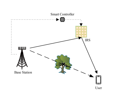
Figure 1: An IRS-assisted mmWave communication system.

For simplicity, we assume that the direct link between the BS and the user is blocked due to poor propagation conditions, and the transmitted signal arrives at the user via propagating through the BS-IRS-user channel. Let $\boldsymbol{G}\in\mathbb{C}^{M\times N}$ and $\boldsymbol{h}\in\mathbb{C}^{M\times 1}$ denote the BS-IRS channel and the IRS-user channel, respectively. The effective channel between the BS and the user can thus be expressed as

$$\boldsymbol{\tilde{h}}^{H} =\boldsymbol{h}^{H}\boldsymbol{\Psi}\boldsymbol{G}=\boldsymbol{\psi}^{T}\text{diag}(\boldsymbol{h}^{H})\boldsymbol{G}\triangleq\boldsymbol{\psi}^{T}\boldsymbol{H}$$ (1)

where $\boldsymbol{\psi}=\text{diag}(\boldsymbol{\Psi})$ and $\boldsymbol{H}\triangleq\text{diag}(\boldsymbol{h}^{H})\boldsymbol{G}$ is referred to as the cascade channel. Let $s$ be the transmitted signal and $\boldsymbol{f}$ be the transmit precoding vector. The signal received at the user can be expressed as

$$y =\boldsymbol{\tilde{h}}^{H}\boldsymbol{f}s+n$$

$$=(\boldsymbol{f}^{T}\otimes\boldsymbol{\psi}^{T})\text{vec}(\boldsymbol{H})s+n\triangleq\boldsymbol{w}\text{vec}(\boldsymbol{H})s+n$$ (2)

where $\boldsymbol{w}\triangleq\boldsymbol{f}^{T}\otimes\boldsymbol{\psi}^{T}$ and $n$ is the additive noise following a complex Gaussian distribution $\mathbb{CN}(0,\sigma^{2})$.

II-B Channel Model

For notational convenience, we first define

$$\boldsymbol{a}(\nu,D)\triangleq[1\phantom{0}\cdots\phantom{0}e^{j(D-1)\nu}]^{T}$$ (3)

We adopt a geometric mmWave channel model [22] to characterize the channel. The BS-IRS channel $\boldsymbol{G}$ can be expressed as

$$\boldsymbol{G} =\sum_{l=1}^{L}\alpha_{l}\boldsymbol{a}_{r}(\theta_{v,l},\theta_{h,l})\boldsymbol{a}_{t}^{H}(\gamma_{l})$$ (4)

where $L$ is the number of paths between the BS and the IRS, $\alpha_{l}$ is the complex gain which is assumed to follow a complex Gaussian distribution $\mathbb{CN}(0,\varpi_{l}^{2})$, $\{\gamma_{l},\theta_{h,l},\theta_{v,l}\}$ are, respectively, the angle of departure (AoD), the elevation and azimuth angle of arrival (AoA) associated with the $l$th path; and $\boldsymbol{a}_{t}(\gamma_{l})$ and $\boldsymbol{a}_{r}(\theta_{v,l},\theta_{h,l})$ are the transmit and receive array response vectors. Specifically, we have

$$\boldsymbol{a}_{t}(\gamma_{l})=\boldsymbol{a}(\nu_{1,l},N)$$ (5)

where $\nu_{1,l}\triangleq\frac{2\pi d}{\lambda}\sin(\gamma_{l})$ with $\lambda$ and $d$ representing the signal wavelength and the antenna spacing, respectively. $\boldsymbol{a}_{r}(\theta_{v,l},\theta_{h,l})$ has a form of a Kronecker product as

$$\boldsymbol{a}_{r}(\theta_{v,l},\theta_{h,l})=\boldsymbol{a}(\nu_{2,l},M_{v})\otimes\boldsymbol{a}(\nu_{3,l},M_{h})$$ (6)

where $\nu_{2,l}\triangleq\frac{2\pi d}{\lambda}\cos(\theta_{v,l})$ and $\nu_{3,l}\triangleq\frac{2\pi d}{\lambda}\sin(\theta_{v,l})\cos(\theta_{h,l})$. Define

$$\boldsymbol{\Sigma}\triangleq \text{diag}(\boldsymbol{\alpha})$$ (7)

$$\boldsymbol{\alpha}\triangleq [\alpha_{1}\ \cdots\ \alpha_{L}]^{T}$$ (8)

$$\boldsymbol{F}_{1}\triangleq [\boldsymbol{a}_{r}(\theta_{v,1},\theta_{h,1}))\phantom{0}\cdots\phantom{0}\boldsymbol{a}_{r}(\theta_{v,L},\theta_{h,L})$$ (9)

$$\boldsymbol{F}_{2}\triangleq [\boldsymbol{a}(\nu_{1,1},N)\ \cdots\ \boldsymbol{a}(\nu_{1,L},N)]$$ (10)

We can express $\boldsymbol{G}$ as

$$\boldsymbol{G}=\boldsymbol{F}_{1}\boldsymbol{\Sigma}\boldsymbol{F}_{2}^{H}$$ (11)

Similarly, the IRS-user channel is characterized as

$$\boldsymbol{h}=\sum_{p=1}^{P}\beta_{p}\boldsymbol{a}_{r}(\psi_{v,p},\psi_{h,p})$$ (12)

where $P$ is the number of paths between the IRS and the user, $\beta_{p}$ is the complex channel gain which follows $\mathbb{CN}(0,\chi_{p}^{2})$, $\{\psi_{v,p},\psi_{h,p}\}$ denotes the elevation and azimuth AoD associated with the $p$th path, and $\boldsymbol{a}_{r}(\psi_{v,p},\psi_{h,p})$ can be expressed as

$$\boldsymbol{a}_{r}(\psi_{v,p},\psi_{h,p})=\boldsymbol{a}(\nu_{4,p},M_{v})\otimes\boldsymbol{a}(\nu_{5,p},M_{h})$$ (13)

where $\nu_{4,p}\!\triangleq\!\frac{2\pi d}{\lambda}\cos(\psi_{v,p})$ and $\nu_{5,p}\!\!\triangleq\!\!\frac{2\pi d}{\lambda}\sin(\psi_{v,p})\cos(\psi_{h,p})$. The IRS-user channel can be written as

$$\boldsymbol{h}=\boldsymbol{F}_{3}\boldsymbol{\beta}$$ (14)

where

$$\boldsymbol{F}_{3}\triangleq [\boldsymbol{a}_{r}(\psi_{v,1},\psi_{h,1})\ \cdots\ \boldsymbol{a}_{r}(\psi_{v,P},\psi_{h,P})]$$ (15)

$$\boldsymbol{\beta}\triangleq [\beta_{1}\ \cdots\ \beta_{P}]^{T}$$ (16)

II-C Motivations

Although I-CSI helps achieve optimal beamforming performance, system optimization based on I-CSI is considered as an intimidating task due to the associated high computational complexity and training overhead as noted in Section I.

To address this challenge, notice that acquiring the I-CSI of the equivalent channel between the BS and the user is much easier and can be accomplished by conventional channel estimation schemes. Inspired by this fact, it is natural to consider a two-timescale beamforming protocol [17]. Specifically, in the long-term time-scale, the reflecting coefficients at the IRS are designed according to the statistical CSI which varies much more slowly than the I-CSI. Then, given fixed passive reflecting coefficients, the BS’s transmit beamforming matrix can be optimally determined based on the instantaneous effective channel in a short-term time-scale.

A prerequisite for such a two-timescale beamforming protocol is to obtain the statistical CSI, i.e. the spatial CCM of the cascade channel. Nevertheless, how to efficiently obtain an estimate of the CCM for IRS-assisted systems has not been fully considered before. The objective of this work is to present a method to estimate the CCM for IRS-aided mmWave systems. Specifically, by exploiting the PSD multi-level Toeplitz and low-rank structure of the CCM, we develop a method which is theoretically guaranteed to attain a reliable estimate of the true CCM with a sample complexity that is much smaller than the dimension of the CCM.

III Downlink Training

In order to estimate the CCM, we employ a downlink training procedure consisting of $T$ time frames. We assume that each time frame has a short period of time so that the channel remains unaltered. Each time frame consists of multiple training time slots, say, $J$ time slots. During the training process, the BS sends a same pilot signal, i.e., $s_{t,j}=1,\ \forall j\in\{1,\cdots,J\}$, to the receiver. The pilot signal is precoded via a transmit precoding vector $\boldsymbol{f}_{t,j}$ that changes over different time frames and different time slots. The signal received at the user can be expressed as

$$y_{t,j} =\boldsymbol{h}_{t}^{H}\boldsymbol{\Psi}_{t,j}\boldsymbol{G}_{t}\boldsymbol{f}_{t,j}+n_{t,j}$$

$$=\boldsymbol{w}_{t,j}\text{vec}\left(\boldsymbol{H}_{t}\right)+n_{t,j}$$ (17)

where $\boldsymbol{h}_{t}$ and $\boldsymbol{G}_{t}$ respectively represent the IRS-user channel and the BS-IRS channel at the $t$th time frame, $\boldsymbol{\Psi}_{t,j}$ is the phase shift matrix that is employed at the $j$th time slot of the $t$th time frame, $n_{t,j}$ is the additive white Gaussian noise, $\boldsymbol{H}_{t}\triangleq\text{diag}(\boldsymbol{h}_{t}^{H})\boldsymbol{G}_{t}$ is referred to as the cascade channel at the $t$th frame, and $\boldsymbol{w}_{t,j}\triangleq\boldsymbol{f}_{t,j}^{T}\otimes\boldsymbol{\psi}_{t,j}^{T}$, in which $\boldsymbol{\psi}_{t,j}=\text{diag}(\boldsymbol{\Psi}_{t,j})$. Define $\boldsymbol{y}_{t}\triangleq[y_{t,1}\cdots y_{t,J}]^{T}$, $\boldsymbol{n}_{t}\triangleq[n_{t,1}\cdots n_{t,J}]^{T}$ and $\boldsymbol{W}_{t}\triangleq[\boldsymbol{w}_{t,1}^{T}\ \cdots\ \boldsymbol{w}_{t,J}^{T}]^{T}$. To facilitate CCM estimation, we employ the same $\boldsymbol{W}=\boldsymbol{W}_{t},\forall t$ for each time frame. Thus the received signal at the $t$th frame can be written in a matrix form as

$$\boldsymbol{y}_{t}=\boldsymbol{W}\text{vec}\left(\boldsymbol{H}_{t}\right)+\boldsymbol{n}_{t}=\boldsymbol{W}\boldsymbol{\bar{h}}_{t}+\boldsymbol{n}_{t}$$ (18)

where $\boldsymbol{\bar{h}}_{t}\triangleq\text{vec}\left(\boldsymbol{H}_{t}\right)$.

As reported by previous studies [23, 24], an important fact about mmWave channels is that the angle parameters such as the AoA and AoD depend only on the relative positions of the BS, the user, and the scatterers, which vary much more slowly than I-CSI. Also, the statistics of the complex path gain keep invariant over an interval that is much longer than the channel coherent time. Hence it is reasonable to make the following basic assumption:

1. The angle parameters and the variances of the path gains, remains unchanged over a long-term period.

Our objective is to obtain an estimate of $\boldsymbol{R}_{h}\triangleq\mathbb{E}[\boldsymbol{\bar{h}}_{t}\boldsymbol{\bar{h}}_{t}^{H}]$ from the received signal $\{\boldsymbol{y}_{t}\}_{t=1}^{T}$. Note that the CCM $\boldsymbol{R}_{h}$ has a dimension of $NM\times NM$. We will show that the knowledge of $\boldsymbol{R}_{h}$ suffices for optimizing the reflecting coefficients at the IRS.

III-A Discussions

Although this paper considers CCM estimation of the downlink channel, the proposed method can be readily applied to the uplink’s CCM estimation. Similar to the downlink training, the uplink training contains $T$ time frames and each time frame consists of $J$ time slots. During the training phase, the user sends a same pilot signal $s_{t,j}=1$ to the BS, where the received signal is combined via a combing vector $\boldsymbol{g}_{t,j}$. The channel in the same time frame is assumed to be time-invariant. Therefore the signal received at the $j$th time slot of the $t$th time frame is given as

$${y}_{t,j}^{u} =\boldsymbol{g}_{t,j}^{H}\boldsymbol{G}_{t}^{H}\boldsymbol{\Psi}_{t,j}\boldsymbol{h}_{t}s_{t,j}+{n}_{t,j}^{u}$$

$$={\boldsymbol{w}}_{t,j}^{u}\text{vec}(\boldsymbol{{H}}_{t}^{u})+{n}_{t,j}^{u}$$ (19)

where $\boldsymbol{G}_{t}$ and $\boldsymbol{h}_{t}$ are, respectively, the IRS-BS channel and the user-IRS channel, ${\boldsymbol{w}}_{t,j}^{u}\triangleq\boldsymbol{\psi}_{t,j}^{T}\otimes\boldsymbol{g}_{t,j}^{H}$ with $\boldsymbol{\psi}_{t,j}=\text{diag}(\boldsymbol{\Psi}_{t,j})$ and $\boldsymbol{H}_{t}^{u}=\boldsymbol{G}_{t}^{H}\text{diag}(\boldsymbol{h}_{t})$. Define $\boldsymbol{y}_{t}^{u}\triangleq[y_{t,1}^{u}\ \cdots\ y_{t,J}^{u}]^{T}$, $\boldsymbol{n}_{t}^{u}\triangleq[n_{t,1}^{u}\ \cdots\ n_{t,J}^{u}]^{T}$, and $\boldsymbol{W}_{t}^{u}\triangleq[(\boldsymbol{w}_{t,1}^{u})^{T}\ \cdots\ (\boldsymbol{w}_{t,J}^{u})^{T}]$. The received signal at the BS can be expressed as

$$\boldsymbol{y}_{t}^{u}=\boldsymbol{{W}}_{t}^{u}\text{vec}(\boldsymbol{H}_{t}^{u})+\boldsymbol{n}_{t}^{u}$$ (20)

If we set $\boldsymbol{{W}}_{t}^{u}$ the same for different time frames, the signal model for the uplink training has a same form as that for the downlink scenario. For time division duplex (TDD) systems, due to the channel reciprocity between opposite links (downlink and uplink), the estimated uplink CCM can be used for downlink precoding/beamforming.

IV Spatial Channel Covariance Matrix Estimation

According to (18), we have

$$\boldsymbol{R}_{y}=\mathbb{E}\{\boldsymbol{y}_{t}\boldsymbol{y}_{t}^{H}\}=\boldsymbol{W}\boldsymbol{R}_{h}\boldsymbol{W}^{H}+\sigma^{2}\boldsymbol{I}$$ (21)

Generally the true covariance matrix $\boldsymbol{R}_{y}$ is unavailable. But it can be estimated via the following sample covariance matrix

$$\boldsymbol{\hat{R}}_{y}=\frac{1}{T}\sum_{t=1}^{T}\boldsymbol{y}_{t}\boldsymbol{y}_{t}^{H}$$ (22)

Intuitively, one can directly estimate $\boldsymbol{R}_{h}$ from $\boldsymbol{\hat{R}_{y}}$ via solving the following least squares problem

$$\text{vec}(\boldsymbol{\hat{R}_{y}})=\left(\boldsymbol{W}^{*}\otimes\boldsymbol{W}\right)\text{vec}({\boldsymbol{R}_{h}})+\text{vec}(\sigma^{2}\boldsymbol{I})$$ (23)

provided that the dimension of $\boldsymbol{\hat{R}_{y}}$ (i.e. $J\times J$) is larger than the dimension of $\boldsymbol{R}_{h}$ (i.e. $MN\times MN$). Nevertheless, the condition $J\geq NM$ is unlikely to be satisfied in practice since the coherence time in mmWave systems is relatively small. Therefore, estimating $\boldsymbol{R}_{h}$ from $\boldsymbol{\hat{R}_{y}}$ is in fact an underdetermined problem, and in order to handle such an issue we have to exploit the structure of $\boldsymbol{R}_{h}$.

IV-A Exploiting The Structure of $\boldsymbol{R}_{h}$

To exploit the structure of $\boldsymbol{R}_{h}$, we first obtain a sparse representation of the cascade channel $\boldsymbol{H}_{t}$. For notational convenience, in the following we will omit the subscript $t$ in $\boldsymbol{H}_{t}$, $\boldsymbol{h}_{t}$ and $\boldsymbol{G}_{t}$. Utilizing the matrix properties, the cascade channel $\boldsymbol{H}$ can be expressed as

$$\boldsymbol{H} =\text{diag}(\boldsymbol{h}^{H})\boldsymbol{G}=\boldsymbol{h}^{*}\bullet\boldsymbol{G}$$

$$=(\boldsymbol{F}_{3}^{*}\boldsymbol{\beta}^{*})\bullet(\boldsymbol{F}_{1}\boldsymbol{\Sigma}\boldsymbol{F}_{2}^{H})$$

$$=\left(\boldsymbol{F}_{3}^{*}\bullet\boldsymbol{F}_{1}\right)\left(\boldsymbol{\beta}^{*}\otimes\left(\boldsymbol{\Sigma}\boldsymbol{F}_{2}^{H}\right)\right)$$

$$=\left(\boldsymbol{F}_{3}^{*}\bullet\boldsymbol{F}_{1}\right)\left(\boldsymbol{\beta}^{*}\otimes\boldsymbol{\Sigma}\right)\boldsymbol{F}_{2}^{H}$$

$$\triangleq\boldsymbol{F}_{4}\boldsymbol{\Pi}\boldsymbol{F}_{2}^{H}$$ (24)

where

$$\boldsymbol{F}_{4}\triangleq \boldsymbol{F}_{3}^{*}\bullet\boldsymbol{F}_{1}$$ (25)

$$\boldsymbol{\Pi}\triangleq \boldsymbol{\beta}^{*}\otimes\boldsymbol{\Sigma}$$ (26)

Note that the $\varsigma$th ($\varsigma=(p-1)L+l$) column of $\boldsymbol{F}_{4}\in\mathbb{C}^{M\times PL}$ is given by

$$\boldsymbol{a}_{r}^{*}(\psi_{v,p},\psi_{h,p})\circ\boldsymbol{a}_{r}(\theta_{v,l},\theta_{h,l})$$

$$\overset{(a)}{=}\left(\boldsymbol{a}^{*}(\nu_{4,p},M_{v})\circ\boldsymbol{a}(\nu_{2,l},M_{v})\right)$$

$$\qquad\quad\otimes\left(\boldsymbol{a}^{*}(\nu_{5,p},M_{h})\circ\boldsymbol{a}(\nu_{3,l},M_{h})\right)$$

$$\triangleq\boldsymbol{a}(\nu_{6,\varsigma},M_{v})\otimes\boldsymbol{a}(\nu_{7,\varsigma},M_{h})$$ (27)

where $\nu_{6,\varsigma}\triangleq\nu_{2,l}-\nu_{4,p}$, $\nu_{7,\varsigma}\triangleq\nu_{3,l}-\nu_{5,p}$, and $(a)$ follows from the property: $(\boldsymbol{A}\otimes\boldsymbol{B})\circ(\boldsymbol{C}\otimes\boldsymbol{D})=(\boldsymbol{A}\circ\boldsymbol{C})\otimes(\boldsymbol{B}\circ\boldsymbol{D})$.

Vectorizing the cascade channel in (24) leads to

$$\text{vec}(\boldsymbol{H})=\text{vec}(\boldsymbol{F}_{4}\boldsymbol{\Pi}\boldsymbol{F}_{2}^{H})\triangleq\boldsymbol{F}\boldsymbol{x}$$ (28)

where $\boldsymbol{F}\triangleq\boldsymbol{F}_{2}^{*}\otimes\boldsymbol{F}_{4}\in\mathbb{C}^{MN\times L^{2}P}$ and $\boldsymbol{x}\triangleq\text{vec}(\boldsymbol{\Pi})\in\mathbb{C}^{L^{2}P}$. $\boldsymbol{F}$ can be further expressed as

$$\boldsymbol{F} =\boldsymbol{F}_{2}^{*}\otimes\boldsymbol{F}_{4}$$

$$=[\boldsymbol{a}^{*}(\nu_{1,1},N)\ \cdots\ \boldsymbol{a}^{*}(\nu_{1,L},N)]$$

$$\qquad\ \otimes\Big{[}\boldsymbol{a}(\nu_{6,1},M_{v})\otimes\boldsymbol{a}(\nu_{7,1},M_{h})\ \cdots$$

$$\qquad\qquad\qquad\qquad\boldsymbol{a}(\nu_{6,LP},M_{v})\otimes\boldsymbol{a}(\nu_{7,LP},M_{h})\Big{]}$$ (29)

Substituting (29) into (28), we have

$$\boldsymbol{\bar{h}}=\text{vec}(\boldsymbol{H})$$

$$=\sum_{l=1}^{L}\sum_{\zeta=1}^{LP}x_{\varrho}\boldsymbol{a}^{*}(\nu_{1,l},N)\otimes\boldsymbol{a}(\nu_{6,\zeta},M_{v})\otimes\boldsymbol{a}(\nu_{7,\zeta},M_{h})$$ (30)

where $x_{\varrho}$ with $\varrho=\zeta+(l-1)LP$ is the $\varrho$th element of $\boldsymbol{x}$. Due to the fact that $\boldsymbol{\Pi}=\boldsymbol{\beta}^{*}\otimes\boldsymbol{\Sigma}$ and $\boldsymbol{\Sigma}$ is a diagonal matrix, there are at most $LP$ non-zeros elements in $\boldsymbol{x}$, and each element in $\boldsymbol{x}$ is given by

$$x_{\varrho}=\left\{\begin{array}[]{ll}\alpha_{l}\beta_{p}^{*},&\varrho\in\boldsymbol{O}\\ 0,&\text{otherwise}\\ \end{array}\right.$$ (33)

where the set $\boldsymbol{O}$ is defined as

$$\Big{\{}(p-1)L+l+(l-1)LP|l\in\{1,\cdots,L\};p\in\{1,\cdots,P\}\Big{\}}$$

Recall that $\alpha_{l}\sim\mathbb{CN}(0,\varpi_{l}^{2})$ and $\beta_{p}\sim\mathbb{CN}(0,\chi_{p}^{2})$, and $\alpha_{l}$ and $\beta_{p}$ are mutually uncorrelated. Therefore for $x_{\varrho}=\alpha_{l}\beta_{p}^{*}$, its mean and variance are given as

$$\mathbb{E}[x_{\varrho}] =0$$

$$\mathbb{E}[x_{\varrho}x_{\varrho}^{*}] =\eta_{\varrho}^{2}\triangleq\varpi_{l}^{2}\chi_{p}^{2}$$ (34)

We see that $\boldsymbol{\bar{h}}$ can be characterized by a geometric channel model. It has $LP$ uncorrelated composite paths in total. The complex gain of each composite path is a random variable with zero mean and finite variance. The angular parameters ($\{\nu_{1,l},\nu_{6,\zeta},\nu_{7,\zeta}\}$) associated with each path are treated as deterministic parameters as angle parameters vary slowly relative to the complex path gains. Hence the channel covariance matrix $\boldsymbol{R}_{h}$ can be expressed as

$$\boldsymbol{R}_{h} =\mathbb{E}(\boldsymbol{\bar{h}}\boldsymbol{\bar{h}}^{H})=\boldsymbol{F}\mathbb{E}(\boldsymbol{x}\boldsymbol{x}^{H})\boldsymbol{F}^{H}$$

$$\overset{(a)}{=}\sum_{{\varrho}=1}^{L^{2}P}\mathbb{E}(x_{\varrho}x_{\varrho}^{*})\boldsymbol{R}_{\varrho}$$

$$=\sum_{{\varrho}\in\boldsymbol{O}}\eta_{\varrho}^{2}\boldsymbol{R}_{\varrho}$$ (35)

where $(a)$ follows from the fact that $\mathbb{E}(\boldsymbol{x}\boldsymbol{x}^{H})$ is a diagonal matrix, and $\boldsymbol{R}_{\varrho}\in\mathbb{C}^{{NM}\times{NM}}$ is defined as

$$\boldsymbol{R}_{\varrho} =\left(\boldsymbol{a}^{*}(\nu_{1,l},N)\boldsymbol{a}^{T}(\nu_{1,l},N)\right)$$

$$\qquad\otimes\left(\boldsymbol{a}(\nu_{6,\zeta},M_{v})\boldsymbol{a}^{H}(\nu_{6,\zeta},M_{v})\right)$$

$$\qquad\qquad\otimes\left(\boldsymbol{a}(\nu_{7,\zeta},M_{h})\boldsymbol{a}^{H}(\nu_{7,\zeta},M_{h})\right)$$ (36)

It can be easily verified that $\boldsymbol{R}_{\varrho}$ is a PSD 3-level Toeplitz matrix. As a result, $\boldsymbol{R}_{h}\in\mathbb{C}^{{NM}\times{NM}}$ is also a PSD 3-level Toeplitz matrix. Although there are $N^{2}M^{2}$ elements in $\boldsymbol{R}_{h}$, owing to the specific structure of PSD 3-level Toeplitz matrix, $\boldsymbol{R}_{h}$ can be characterized by $(2N-1)(2M_{v}-1)(2M_{h}-1)$ parameters which can be represented by a third-order tensor $\boldsymbol{V}\in\mathbb{C}^{(2N-1)\times(2M_{v}-1)\times(2M_{h}-1)}$, i.e. we can write $\boldsymbol{R}_{h}=\mathbb{T}_{3}(\boldsymbol{V})$. How to map a third-order tensor to a 3-level Toeplitz can be found in Appendix D. Furthermore, from (35), we know that $\boldsymbol{R}_{h}$ can be represented by a summation of $LP$ rank-one matrices. Due to the sparse scattering characteristics of mmWave channels, $LP$ is usually much smaller than the dimension of $\boldsymbol{R}_{h}$ (i.e., $NM$), meaning that $\boldsymbol{R}_{h}$ has a low-rank structure.

Utilizing the PSD 3-level Toeplitz structure and the low-rank property of $\mathbb{T}_{3}(\boldsymbol{V})$, the estimation of $\boldsymbol{R}_{h}$ can be cast into the following low-rank structured covariance reconstruction problem:

$$\boldsymbol{\hat{R}}_{h}= \arg\min_{\mathbb{T}_{3}(\boldsymbol{V})}\ \frac{1}{2}\left\|\boldsymbol{\hat{R}}_{y}-\boldsymbol{W}\mathbb{T}_{3}(\boldsymbol{V})\boldsymbol{W}^{H}\right\|_{F}^{2}+\lambda\text{rank}(\mathbb{T}_{3}(\boldsymbol{V}))$$

$$\qquad\text{s.t.}\quad\mathbb{T}_{3}(\boldsymbol{V})\succcurlyeq 0$$ (37)

where $\lambda$ is a regularization parameter to balance the tradeoff between data fitting and low-rankness. Nonetheless, such a problem is generally NP-hard due to the rank function. To make it tractable, we resort to convex relaxation to replace $\text{rank}(\mathbb{T}_{3}(\boldsymbol{V}))$ with the nuclear-norm of $\mathbb{T}_{3}(\boldsymbol{V})$. Since $\mathbb{T}_{3}(\boldsymbol{V})$ is confined to be a PSD matrix, its nuclear norm is equivalent to its trace. Consequently, the resulting optimization can be given by

$$\boldsymbol{\hat{R}}_{h}= \arg\min_{\mathbb{T}_{3}(\boldsymbol{V})}\quad\frac{1}{2}\left\|\boldsymbol{\hat{R}}_{y}-\boldsymbol{W}\mathbb{T}_{3}(\boldsymbol{V})\boldsymbol{W}^{H}\right\|_{F}^{2}+\lambda\text{tr}(\mathbb{T}_{3}(\boldsymbol{V}))$$

$$\qquad\text{s.t.}\qquad\mathbb{T}_{3}(\boldsymbol{V})\succcurlyeq 0$$ (38)

The above optimization is a convex semidefinite programming (SDP) problem which can be solved by many standard off-the-shelf solvers, e.g., CVX. Unfortunately, these solvers are usually computationally expensive. To reduce the computational complexity, we develop an alternating direction method of multipliers (ADMM) algorithm for solving  (38) in the next section.

IV-B ADMM-Based Algorithm

To solve (38), we first introduce two auxiliary variables, $\boldsymbol{A}$ and $\boldsymbol{B}$, and reformulate (38) into the following optimization

$$\{\boldsymbol{\hat{V}},\boldsymbol{\hat{A}},\boldsymbol{\hat{B}}\}= \arg\min_{\boldsymbol{V},\boldsymbol{A},\boldsymbol{B}}\ \Big{(}\frac{1}{2}\left\|\boldsymbol{\hat{R}}_{y}-\boldsymbol{W}\boldsymbol{A}\boldsymbol{W}^{H}\right\|_{F}^{2}$$

$$\qquad\qquad\qquad+\lambda\text{tr}(\boldsymbol{A})+\mathbb{I}_{\infty}(\boldsymbol{B}\succcurlyeq 0)\Big{)}$$

$$\qquad\text{s.t.}\qquad\boldsymbol{A}=\mathbb{T}_{3}(\boldsymbol{V}),\ \boldsymbol{B}=\boldsymbol{A},\$$ (39)

where $\mathbb{I}_{\infty}(a)$ is an indicator function defined as

$$\mathbb{I}_{\infty}(a)=\left\{\begin{array}[]{ll}0,&\quad\text{if $a$ is true}\\ \infty,&\quad\text{otherwise}\end{array}\right.$$ (42)

The augmented Lagrangian of the above optimization is read as

$$\mathcal{L}(\boldsymbol{V},\boldsymbol{A},\boldsymbol{B},\boldsymbol{\Upsilon},\boldsymbol{\Lambda})$$

$$=\frac{1}{2}\left\|\boldsymbol{\hat{R}}_{y}-\boldsymbol{W}\boldsymbol{A}\boldsymbol{W}^{H}\right\|_{F}^{2}+\lambda\text{tr}(\boldsymbol{A})$$

$$\qquad+\left\langle\boldsymbol{\Upsilon},\boldsymbol{A}-\mathbb{T}_{3}(\boldsymbol{V})\right\rangle+\frac{\eta}{2}\left\|\boldsymbol{A}-\mathbb{T}_{3}(\boldsymbol{V})\right\|_{F}^{2}$$

$$\qquad\quad+\left\langle\boldsymbol{\Lambda},\boldsymbol{B}-\boldsymbol{A}\right\rangle+\frac{\rho}{2}\left\|\boldsymbol{B}-\boldsymbol{A}\right\|_{F}^{2}+\mathbb{I}_{\infty}(\boldsymbol{B}\succcurlyeq 0)$$ (43)

where $\left\langle\boldsymbol{A},\boldsymbol{B}\right\rangle$ is defined as $\text{Re}\big{(}\text{Tr}(\boldsymbol{B}^{H}\boldsymbol{A})\big{)}$, $\boldsymbol{\Upsilon}$ and $\boldsymbol{\Lambda}$ are the dual parameters, and $\eta,\rho>0$ are the penalty parameters. According to the updating rule of the ADMM algorithm, it consists of solving the following sub-problems:

$$\boldsymbol{\hat{A}}^{k+1} =\arg\min_{\boldsymbol{A}}\ \mathcal{L}(\boldsymbol{V}^{k},\boldsymbol{A},\boldsymbol{B}^{k},\boldsymbol{\Upsilon}^{k},\boldsymbol{\Lambda}^{k})$$ (44)

$$\boldsymbol{\hat{V}}^{k+1} =\arg\min_{\boldsymbol{V}}\ \mathcal{L}(\boldsymbol{V},\boldsymbol{A}^{k+1},\boldsymbol{B}^{k},\boldsymbol{\Upsilon}^{k},\boldsymbol{\Lambda}^{k})$$ (45)

$$\boldsymbol{\hat{B}}^{k+1} =\arg\min_{\boldsymbol{B}}\ \mathcal{L}(\boldsymbol{V}^{k+1},\boldsymbol{A}^{k+1},\boldsymbol{B},\boldsymbol{\Upsilon}^{k},\boldsymbol{\Lambda}^{k})$$ (46)

$$\boldsymbol{\Upsilon}^{k+1} =\boldsymbol{\Upsilon}^{k}+\eta\big{(}\boldsymbol{A}^{k+1}-\mathbb{T}_{3}(\boldsymbol{V}^{k+1})\big{)}$$ (47)

$$\boldsymbol{\Lambda}^{k+1} =\boldsymbol{\Lambda}^{k}+\rho\big{(}\boldsymbol{B}^{k+1}-\boldsymbol{A}^{k+1}\big{)}$$ (48)

Update of $\boldsymbol{A}$: We first solve the sub-problem (44). Calculating the derivative of $\mathcal{L}(\boldsymbol{V}^{k},\boldsymbol{A},\boldsymbol{B}^{k},\boldsymbol{\Upsilon}^{k},\boldsymbol{\Lambda}^{k})$ with respect to $\boldsymbol{A}$, we have

$$\nabla_{\boldsymbol{A}}\mathcal{L} =(\boldsymbol{W}^{H}\boldsymbol{W})\boldsymbol{A}(\boldsymbol{W}^{H}\boldsymbol{W})^{H}+(\eta-\rho)\boldsymbol{A}-\eta\mathbb{T}_{3}(\boldsymbol{V}^{k})$$

$$\qquad+\rho\boldsymbol{B}^{k}-\boldsymbol{W}^{H}\boldsymbol{\hat{R}}_{y}\boldsymbol{W}+\boldsymbol{\Upsilon}^{k}-\boldsymbol{\Lambda}^{k}+\lambda\boldsymbol{I}$$ (49)

By setting $\nabla_{\boldsymbol{A}}\mathcal{L}$ to $0$, we can update $\boldsymbol{A}$ via solving the following linear equation

$$\boldsymbol{\Xi}\boldsymbol{A}\boldsymbol{\Xi}^{H}+\kappa\boldsymbol{A}=\boldsymbol{C}$$ (50)

where $\boldsymbol{C}=\eta\mathbb{T}_{3}(\boldsymbol{V}^{k})-\rho\boldsymbol{B}^{k}+\boldsymbol{W}^{H}\boldsymbol{\hat{R}}_{y}\boldsymbol{W}-\lambda\boldsymbol{I}-\boldsymbol{\Upsilon}^{k}+\boldsymbol{\Lambda}^{k}$, $\kappa=\eta-\rho$ and $\boldsymbol{\Xi}=\boldsymbol{W}^{H}\boldsymbol{W}$. Clearly, $\boldsymbol{A}$ can be solved via

$$(\boldsymbol{\Xi}^{*}\otimes\boldsymbol{\Xi}+\kappa\boldsymbol{I})\text{vec}(\boldsymbol{A})=\text{vec}(\boldsymbol{C})$$ (51)

Nevertheless, this approach has a computational complexity of $\mathcal{O}(N^{6}M^{6})$. To reduce the computational complexity, we propose a more computationally-efficient approach to solve (50). Since $\boldsymbol{\Xi}=\boldsymbol{W}^{H}\boldsymbol{W}$, $\boldsymbol{\Xi}$ can be diagonalized via the eigen-decomposition (EVD), i.e.,

$$\boldsymbol{\Xi}=\boldsymbol{A}_{1}\boldsymbol{A}_{2}\boldsymbol{A}_{1}^{H}$$ (52)

where $\boldsymbol{A}_{2}$ is a diagonal matrix and $\boldsymbol{A}_{1}$ is a unitary matrix (meaning $\boldsymbol{A}_{1}^{H}=\boldsymbol{A}_{1}^{-1}$). Substituting (52) into (50) results in

$$\boldsymbol{A}_{1}\boldsymbol{A}_{2}\boldsymbol{A}_{1}^{H}\boldsymbol{A}(\boldsymbol{A}_{1}\boldsymbol{A}_{2}\boldsymbol{A}_{1}^{H})^{H}+\kappa\boldsymbol{A}=\boldsymbol{C}$$ (53)

By defining $\boldsymbol{A}_{3}\triangleq\boldsymbol{A}_{1}^{H}\boldsymbol{A}\boldsymbol{A}_{1}$ and $\boldsymbol{C}_{1}\triangleq\boldsymbol{A}_{1}^{H}\boldsymbol{C}\boldsymbol{A}_{1}$, we can express (53) as

$$\boldsymbol{A}_{2}\boldsymbol{A}_{3}\boldsymbol{A}_{2}+\kappa\boldsymbol{A}_{3}=\boldsymbol{C}_{1}$$ (54)

Since $\boldsymbol{A}_{2}$ is a diagonal matrix, we can explicitly solve (54) in an elementwise manner. Once $\boldsymbol{A}_{3}$ is obtained, $\boldsymbol{A}$ can be simply reconstructed as

$$\boldsymbol{A}=\boldsymbol{A}_{1}\boldsymbol{A}_{3}\boldsymbol{A}_{1}^{H}$$ (55)

Update of $\boldsymbol{V}$: Keeping the terms that only depend on $\boldsymbol{V}$ in (45), we have

$$\boldsymbol{\hat{V}}^{k+1}= \arg\min_{\boldsymbol{V}}\ \frac{\eta}{2}\text{Tr}\left(\mathbb{T}_{3}^{H}(\boldsymbol{V})\mathbb{T}_{3}(\boldsymbol{V})\right)$$

$$\qquad\quad\ -\text{Re}\left(\text{Tr}\big{(}(\boldsymbol{\Upsilon}^{k}+\eta\boldsymbol{A}^{k+1})^{H}\mathbb{T}_{3}(\boldsymbol{V})\big{)}\right)$$ (56)

Directly taking derivative with respect to $\boldsymbol{V}$ is difficult. Nevertheless, the elements in $\boldsymbol{V}$ can be optimized separately. To this end, we reshape $\boldsymbol{V}\in\mathbb{C}^{(2N-1)\times(2M_{v}-1)\times(2M_{h}-1)}$ to a vector $\boldsymbol{v}\in\mathbb{C}^{(2N-1)(2M_{v}-1)(2M_{h}-1)}$. Also, we define an index set $\mathbb{I}_{v_{l}}$ as

$$\mathbb{I}_{v_{l}} =\{(i,j)|\mathbb{T}_{3}(\boldsymbol{V})(i,j)\equiv v_{l}\}$$ (57)

for all $l\in\{1,\cdots,(2N-1)(2M_{v}-1)(2M_{h}-1)\}$. The cardinality of the set $\mathbb{I}_{v_{l}}$ is denoted by $|\mathbb{I}_{v_{l}}|$. Based on this definition, the terms that only depend on $v_{l}$ in the cost function (56) can be rewritten as

$$\hat{v}_{l}^{k+1}=\arg\min_{v_{l}}\frac{\eta|\mathbb{I}_{v_{l}}|}{2}v_{l}v_{l}^{*}-\bigg{(}\sum_{(i,j)\in\mathbb{I}_{v_{l}}}\text{Re}\left(\Delta^{*}(i,j)v_{l}\right)\bigg{)}$$ (58)

where $\Delta\triangleq\boldsymbol{\Upsilon}^{k}+\eta\boldsymbol{A}^{k+1}$. It is clear that $\hat{v}_{l}^{k+1}$ is given by

$$\hat{v}_{l}^{k+1}=\frac{1}{\eta|\mathbb{I}_{v_{l}}|}\bigg{(}\sum_{(i,j)\in\mathbb{I}_{v_{l}}}\Delta(i,j)\bigg{)}$$ (59)

Update of $\boldsymbol{B}$: The optimization in (46) is equivalent to

$$\boldsymbol{\hat{B}}^{k+1}=\arg\min_{\boldsymbol{B}}\ \frac{\rho}{2}\text{Tr}(\boldsymbol{B}\boldsymbol{B}^{H})+\text{Re}(\text{Tr}((\boldsymbol{\Lambda}^{k}-\rho\boldsymbol{A}^{k+1})^{H}\boldsymbol{B}))$$

$$\qquad+\mathbb{I}_{\infty}(\boldsymbol{B}\succcurlyeq 0)$$ (60)

The last term in (60) makes the optimization problem intractable. To handle this issue, we propose a two-step solution. Specifically, we first ignore the positive semi-definite constraint and solve the following optimization problem

$$\boldsymbol{\tilde{B}}=\arg\min_{\boldsymbol{B}}\ \frac{\rho}{2}\text{Tr}(\boldsymbol{B}\boldsymbol{B}^{H})+\text{Re}(\text{Tr}((\boldsymbol{\Lambda}^{k}-\rho\boldsymbol{A}^{k+1})^{H}\boldsymbol{B}))$$ (61)

which gives

$$\boldsymbol{\tilde{B}}=\boldsymbol{A}^{k+1}-\boldsymbol{\Lambda}^{k}/\rho$$ (62)

Then we calculate $\boldsymbol{\hat{B}}^{k+1}$ by projecting $\boldsymbol{\tilde{B}}$ onto the positive semi-definite cone, which is equivalent to setting all negative eigenvalues of $\boldsymbol{\tilde{B}}$ to zero.

V Performance Analysis of The CCM Estimator

In this section, we analyze the estimation performance of the CCM estimator (38). Specifically, we are interested in quantifying the amount of training overhead required to achieve a reliable estimate of the true CCM $\boldsymbol{R}_{h}$. To facilitate our analysis, we consider the noise-free case, i.e., $\sigma^{2}=0$ and $\boldsymbol{R}_{y}=\boldsymbol{W}\boldsymbol{R}_{h}\boldsymbol{W}^{H}$. In the following we use $\boldsymbol{R}_{h}$ and $\mathbb{T}_{3}(\boldsymbol{V})$ interchangeably since these two essentially have the same meaning.

Suppose $\mathbb{T}_{3}(\boldsymbol{X})\!\in\!\mathbb{C}^{I_{1}I_{2}I_{3}\times I_{1}I_{2}I_{3}}$ is a 3-level Toeplitz matrix parameterized by a tensor $\boldsymbol{X}\in\mathbb{C}^{(2I_{1}-1)\times(2I_{2}-1)\times(2I_{3}-1)}$. For any matrix $\boldsymbol{M}\in\mathbb{C}^{I\times I_{1}I_{2}I_{3}}$, $\boldsymbol{\check{M}}\in\mathbb{C}^{I^{2}\times(2I_{1}-1)(2I_{2}-1)(2I_{3}-1)}$ is referred to as the transforming matrix of $\boldsymbol{M}$ if it satisfies

$$\boldsymbol{\check{M}}\boldsymbol{x}=\text{vec}(\boldsymbol{M}\mathbb{T}_{3}(\boldsymbol{X})\boldsymbol{M}^{H})$$ (63)

where $\boldsymbol{x}$ is a vector by reshaping $\boldsymbol{X}$ into a vector. In addition, define $r_{e}(\boldsymbol{A})\triangleq\frac{\text{Tr}(\boldsymbol{A})}{\|\boldsymbol{A}\|_{2}}$ as the effective rank of matrix $\boldsymbol{A}$. Our result is summarized as follows.

Theorem 1

Let $\boldsymbol{V}\in\mathbb{C}^{(2N-1)\times(2M_{v}-1)\times(2M_{h}-1)}$ be the ground truth and $\boldsymbol{\hat{V}}\in\mathbb{C}^{(2N-1)\times(2M_{v}-1)\times(2M_{h}-1)}$ be the solution of (38). Given observations $\{\boldsymbol{y}_{t}\}_{t=1}^{T}$, and set

$$J\geq u\triangleq\sqrt{(2N-1)(2M_{v}-1)(2M_{h}-1)}$$ (64)

and

$$\lambda\geq c\|\boldsymbol{W}\|_{F}^{2}\|\boldsymbol{R}_{y}\|_{2}\text{max}\{\sqrt{\tilde{\delta}},\tilde{\delta}\}$$ (65)

where $c$ is a constant and $\tilde{\delta}$ is defined as

$$\tilde{\delta}\triangleq\frac{r_{e}(\boldsymbol{R}_{y})\log(TJ)}{T}$$ (66)

then with probability at least $1-4T^{-1}$, the average per-entry root mean square error (RMSE) of the solution to (38) satisfies

$$\frac{1}{u}\|\boldsymbol{\hat{V}}-\boldsymbol{V}\|_{F}\leq\frac{16\lambda\sqrt{r}}{\sigma^{2}_{\text{min}}(\boldsymbol{\check{W}})}\frac{\sqrt{NM}}{u}$$ (67)

where $r$ is the rank of $\boldsymbol{R}_{h}$, $\boldsymbol{\check{W}}$ is the transforming matrix of $\boldsymbol{W}$, and $\sigma_{\text{min}}(\boldsymbol{\check{W}})$ denotes the smallest singular value of $\boldsymbol{\check{W}}$.

Proof:

See Appendix A. ∎

The above theorem is a generalization of Theorem 4 in [25]. Specifically, [25] analyzes the structured covariance estimation performance under a partial observation framework where the aim is to recover the complete CCM from a submatrix of the sample CCM. Theorem 1 generalizes this partial observation model to an arbitrarily linear compression model in which we do not have direct access to the entries of the sample CCM; instead, only the sample covariance matrix $\boldsymbol{\hat{R}}_{y}$ is available. Also, the CCM in this work has a multi-level Toeplitz structure, which is different from that of [25].

Recalling $M=M_{v}M_{h}$, the term $\sqrt{NM}/u$ in (67) tends to be a constant for sufficiently large values of $M$ and $N$. Therefore, the average per-entry RMSE is upper bounded by $\lambda\sqrt{r}$ times a scale factor. According to (65), we know that

$$\lambda\sqrt{r}\geq\bar{u}\triangleq c\sqrt{r}\|\boldsymbol{W}\|_{F}^{2}\|\boldsymbol{R}_{y}\|_{2}\text{max}\{\sqrt{\tilde{\delta}},\tilde{\delta}\}$$ (68)

Therefore, in our optimization problem (38), we set $\lambda=\bar{u}/\sqrt{r}$ such that the average pre-entry RMSE of $\boldsymbol{V}$ has the smallest upper bound, i.e.,

$$\frac{1}{u}\|\boldsymbol{\hat{V}}-\boldsymbol{V}\|_{F}$$

$$\leq\frac{\sqrt{NM}}{u}\frac{16\bar{u}}{\sigma^{2}_{\text{min}}(\boldsymbol{\check{W}})}$$

$$=\frac{\sqrt{NM}}{u}\frac{16c\|\boldsymbol{W}\|_{F}^{2}\|\boldsymbol{R}_{y}\|_{2}\text{max}\{\sqrt{r\tilde{\delta}},\sqrt{r}\tilde{\delta}\}}{\sigma^{2}_{\text{min}}(\boldsymbol{\check{W}})}$$ (69)

From (69), we can see that the average pre-entry RMSE vanishes as long as $r\tilde{\delta}$ tends to $0$. To this objective, it can be verified that the number of time frames $T$ should be in the order of $r_{e}(\boldsymbol{R}_{y})r\log(J)$ or in the order of $r^{2}\log(J)$ since the effective rank of a matrix is no greater than its true rank, i.e. $r_{e}(\boldsymbol{R}_{y})\leq r$ [26]. To see why $r\tilde{\delta}$ tends to $0$ when $T\sim\mathcal{O}(r^{2}\log(J))$, let $T=\tau r^{2}\log(J)$, where $\tau$ is a constant. In this case, we have

$$r\tilde{\delta}\leq\frac{\log(\tau r^{2}\log(J))}{\tau\log(J)}$$ (70)

where the right-hand side of the above inequality decreases to a small value as $\tau$ increases. In summary, when the number of time frames $T$ is in the order of $r^{2}\log(J)$, the average per-entry RMSE can be upper bounded by an arbitrarily small value, which means that we can obtain a reliable estimate of the true CCM $\boldsymbol{R}_{h}$. Note that our performance guarantee is non-asymptotic and holds for a finite number of measurement vectors. In other words, the result has accounted for the covariance estimation error due to finite samples.

Recall that the proposed downlink training protocol consists of $T$ time frames, and each time frame comprises $J$ time slots. Thus the total amount of training overhead is $TJ$. Since the number of time slots $J$ has to satisfy (64), which means that $J$ is on the order of $\sqrt{NM}$. Therefore, the total amount of training overhead is at the order of $r^{2}\sqrt{NM}\log(NM)$. Note that here $r=PL$ is the rank of $\boldsymbol{R}_{h}$. In mmWave systems, due to sparse scattering characteristics, both $P$ and $L$ are relatively small. Hence $r$ is generally far less than $NM$. Based on this, we can conclude that when the total number of training symbols is in the order of $\sqrt{NM}\log{NM}$, we can provide a reliable estimate of the CCM $\boldsymbol{R}_{h}$. Note that $\sqrt{NM}\log{NM}$ is much smaller than the dimension of $\boldsymbol{R}_{h}$ (i.e., $N^{2}M^{2}$).

VI Two-Timescale Beamforming Based on Estimated CCM

In this section, we discuss how to perform two-timescale beamforming based on the estimated CCM. For the considered point-to-point IRS-assisted mmWave system, the received signal at the user can be expressed as

$$y_{t}=\boldsymbol{h}^{H}\boldsymbol{\Psi}\boldsymbol{G}\boldsymbol{f}s_{t}+n_{t}$$ (71)

where $s_{t}$ is the transmitted symbol satisfying $\mathbb{E}(|s_{t}|^{2})=1$, $\boldsymbol{f}$ is the precoding vector, and $n_{t}\sim\mathbb{CN}(0,\sigma^{2})$ denotes the zero-mean complex Gaussian noise. The achievable spectral efficiency can be expressed as

$$R=\log_{2}(1+{|\boldsymbol{h}^{H}\boldsymbol{\Psi}\boldsymbol{G}\boldsymbol{f}|^{2}}/{\sigma^{2}})$$ (72)

To circumvent the need for the I-CSI $\boldsymbol{h}$ and $\boldsymbol{G}$, we adopt a two-timescale beamforming approach. Specifically, in the long-term time-scale, the reflecting coefficients at the IRS are optimized based on the estimated CCM. Then, given fixed passive reflecting coefficients, the BS’s transmit beamforming matrix can be optimally determined based on the instantaneous effective channel in a short-term time-scale. Such a joint beamforming problem can be formulated into the following optimization:

$$\max_{\boldsymbol{\psi}}\ \ \mathbb{E}\bigg{\{}\max_{\boldsymbol{f}}R\bigg{\}}$$

$$s.t.\quad |\psi_{m}|=1\ \ \forall m\in\{1,\cdots,M\}$$

$$\|\boldsymbol{f}\|^{2}\leq P_{\text{max}}$$ (73)

where $\boldsymbol{\psi}=\text{diag}(\boldsymbol{\Psi})$ with $\psi_{m}$ as its $m$th element and $P_{\text{max}}$ is the total transmit power budget. The optimization problem in (73) has two levels. The inner one is the rate-maximization problem with respect to $\boldsymbol{f}$. This is implemented in each channel realization with the given phase shift matrix $\boldsymbol{\Psi}$. The outer one is an expectation maximization problem over the IRS phase shift coefficients in which the expectation of the achievable rate is taken over all possible channel realizations.

When $\boldsymbol{\Psi}$ is given, the optimal precoding vector is the maximum-ratio transmission (MRT) which is explicitly given as

$$\boldsymbol{f}=\sqrt{P_{\text{max}}}\frac{(\boldsymbol{h}^{H}\boldsymbol{\Psi}\boldsymbol{G})^{H}}{\|\boldsymbol{h}^{H}\boldsymbol{\Psi}\boldsymbol{G}\|_{2}}$$ (74)

Substituting (74) into (73), we arrive at the following optimization problem which is only related to $\boldsymbol{\Psi}$:

$$\max_{\boldsymbol{\psi}}\ \ \mathbb{E}\left\{\log_{2}(1+P_{\text{max}}\|\boldsymbol{h}^{H}\boldsymbol{\Psi}\boldsymbol{G}\|^{2}/\sigma^{2})\right\}$$

$$s.t.\quad |\psi_{m}|=1\ \ \forall m\in\{1,\cdots,M\}$$ (75)

Directly solving (75) is intractable. The major reason is that its cost function is the expectation of a logarithmic function, which in general does not have an explicit expression. To handle this issue, we resort to maximize its tight upper bound, which is given by [17]

$$\mathbb{E}\{\log_{2}(1+P_{\text{max}}\|\boldsymbol{h}^{H}\boldsymbol{\Psi}\boldsymbol{G}\|^{2}/\sigma^{2})\}$$

$$\qquad\qquad\leq\log_{2}(1+P_{\text{max}}\mathbb{E}\{\|\boldsymbol{h}^{H}\boldsymbol{\Psi}\boldsymbol{G}\|^{2}\}/\sigma^{2})$$ (76)

Note that the upper bound shown in (76) is sufficiently tight and thus is a good approximation of the original objective function, especially when $P_{\text{max}}/\sigma^{2}$ is large. Such an optimization trick has been used in existing literatures, e.g.[17, 16]. Maximizing the upper bound yields the following optimization:

$$\max_{\boldsymbol{\psi}}\ \ \mathbb{E}(\|\boldsymbol{h}^{H}\boldsymbol{\Psi}\boldsymbol{G}\|^{2})$$

$$s.t.\quad |\psi_{m}|=1\ \ \forall m\in\{1,\cdots,M\}$$ (77)

where $\mathbb{E}(\|\boldsymbol{h}^{H}\boldsymbol{\Psi}\boldsymbol{G}\|^{2})$ is given by

$$\mathbb{E}(\|\boldsymbol{h}^{H}\boldsymbol{\Psi}\boldsymbol{G}\|^{2}) =\mathbb{E}(\|\boldsymbol{\psi}^{T}\boldsymbol{H}\|^{2})$$

$$=\boldsymbol{\psi}^{T}\mathbb{E}(\boldsymbol{H}\boldsymbol{H}^{H})\boldsymbol{\psi}^{*}$$

$$=\boldsymbol{\psi}^{T}\boldsymbol{\bar{R}}_{h}\boldsymbol{\psi}^{*}$$ (78)

in which $\boldsymbol{\bar{R}}_{h}$ is the covariance matrix of the cascade channel $\boldsymbol{H}$. Note that $\boldsymbol{\bar{R}}_{h}=\mathbb{E}(\boldsymbol{H}\boldsymbol{H}^{H})$ and $\boldsymbol{R}_{h}=\mathbb{E}(\text{vec}(\boldsymbol{H})\text{vec}(\boldsymbol{H})^{H})$. Therefore, $\boldsymbol{\bar{R}}_{h}$ can be directly obtained from $\boldsymbol{R}_{h}$. Specifically, the $(i,j)$th element of $\boldsymbol{\bar{R}}_{h}$ can be calculated by

$$\boldsymbol{\bar{R}}_{h}(i,j)=\sum_{k=1}^{N}\boldsymbol{R}_{h}(i+(k-1)M,j+(k-1)M)$$ (79)

for $1\leq i,j\leq M$.

The optimization problem (77) with its cost function given in (78) is a nonconvex quadratically constrained quadratic problem, and it can be relaxed as the following semidefinite programming (SDP) problem

$$\max_{\boldsymbol{V}}\ \text{Tr}(\boldsymbol{\bar{R}}_{h}\boldsymbol{V})$$

$$s.t.\ {V}_{ii}=1$$

$$\boldsymbol{V}\succcurlyeq 0$$

$$\text{rank}(\boldsymbol{V})=1$$ (80)

where $\boldsymbol{V}=\boldsymbol{\psi}^{*}\boldsymbol{\psi}^{T}$ is a rank-one matrix and ${V}_{ii}$ is the $i$th diagonal element of $\boldsymbol{V}$. When ignoring the rank-one constraint, (80) can be immediately solved by the off-the-shelf SDR programming toolboxes, e.g., the CVX. After obtaining the optimal solution $\boldsymbol{V}$, we need to find a feasible solution $\boldsymbol{v}$ from $\boldsymbol{V}$. One efficient approach is the Gaussian randomization approximation solution [27], and the detailed procedures can be found within.

VII Simulation Results

In this section, we present simulation results to illustrate the effectiveness of the proposed low-rank PSD Toeplitz-structured CCM (LRT-CCM) estimation method. We compare our method with the conventional CCM estimation approach which estimates the channel at each time frame and then reconstructs the CCM with these estimated channel samples. Such an approach is referred to as the conventional CCM estimation method. For this approach, we use the compressed sensing-based method [5] to estimate the channel at each time frame.

In our simulations, the BS employs a uniform linear array (ULA) of $N=8$ antennas and the IRS is a planar array with $M_{v}\times M_{h}=16\times 16$ reflecting elements. The three-dimensional coordinates of the BS, the IRS, and the user are set to $(5,0,10)$, $(0,50,20)$ and $(10,60,1.8)$, respectively. The BS-IRS channel and the IRS-user channel are generated according to (4) and (12), respectively. The number of the signal paths is set to $L=P=3$, and each channel comprises an LOS path and two NLOS paths. The corresponding angles (including AoAs and AoDs) of the LOS paths are determined by the geometry configuration, and the associated complex gains of the LOS paths are generated according to a complex Gaussian distribution $\mathbb{CN}(0,10^{-0.1\kappa})$, where $\kappa=61.4+29.2\log_{10}(d)+\epsilon$ with $d$ denoting the length of the path and $\epsilon$ being a random variable following $\mathbb{N}(0,(8.7\text{dB})^{2})$. The angles associated with the NLOS paths are randomly selected from the interval $[-\pi,\pi]$. The channel coefficients of these NLOS paths follow a distribution $\mathbb{CN}(0,\delta^{2})$, where $\delta$ is determined by the Rician factor (i.e., the ratio of the energy of the LOS path to that of all NLOS paths). We set the Rician factor to $10$ dB and the transmitted power to $P_{\max}=30\text{dBm}$. The signal-to-noise ratio (SNR) is defined as

$$\text{SNR}=\mathbb{E}\left(10\log_{10}\left({\varsigma^{2}}/{\sigma^{2}}\right)\right)$$ (81)

where $\varsigma^{2}$ is the received signal power.

We evaluate the CCM estimation performance via the relative efficiency metric (REM), which is widely adopted [28, 29, 30] and defined as

$$\eta=\frac{\text{tr}(\boldsymbol{U}_{1}^{H}\boldsymbol{R}_{h}\boldsymbol{U}_{1})}{\text{tr}(\boldsymbol{U}_{2}^{H}\boldsymbol{R}_{h}\boldsymbol{U}_{2})}$$ (82)

where $\boldsymbol{U}_{1}$ and $\boldsymbol{U}_{2}$ are, respectively, the matrices constructed by the eigenvectors of the estimated CCM $\boldsymbol{\hat{R}}_{h}$ and the eigenvectors of the true CCM $\boldsymbol{R}_{h}$. Clearly, a higher value of $\eta$ indicates a more accurate CCM estimate. The value $1-\eta$ means the lost of the signal power due to the mismatch between the optimal beamformer and the estimated one. All results are averaged over 50 independent Monte Carlo runs.

Fig. 2(a) plots the REMs of different methods as a function of the SNR, where the number of time slots $J$ is set to $120$ and the number of time frames $T$ is set to $100$. We see that our proposed method presents a substantial performance improvement over the conventional CCM estimation method, particularly in the low SNR regime. In fact, our proposed method can still provide a reliable CCM estimate even when the SNR is below -10dB, whereas the conventional CCM estimation method performs poorly in such a low SNR region. In Fig. 2(b), we plot the achievable rate attained by the two-timescale beamforming scheme based on the estimated CCM. To better evaluate the performance, we also include the achievable rates attained by the two-timescale beamforming scheme based on the true CCM, the two-timescale beamforming scheme in which the reflecting coefficients are randomly chosen from a unit circle (referred to as random passive beamforming), and the joint beamforming scheme [31] that utilizes the true I-CSI. Note that the beamforming approach [31] that exploits the I-CSI provides an upper bound on the performance that is achievable by any two-timescale beamforming schemes.

Several points can be made from Fig. 2(b). First, our proposed method incurs only a very mild performance loss as compared with the two-timescale beamforming scheme based on the true CCM. This result indicates that the proposed method can yield a CCM estimate that is good enough for subsequent beamforming. Second, the two-timescale beamforming scheme can achieve performance close to that of the beamforming method that utilizes the I-CSI, which demonstrates the effectiveness of the two-timescale beamforming scheme. Lastly, all methods present a substantial performance advantage over the random passive beamforming scheme.

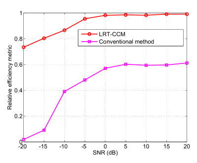
(a) REM

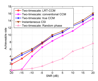
(b) Achievable rate

Figure 2: REMs and achievable rates of respective methods, where we set $T=100$ and $J=120$.

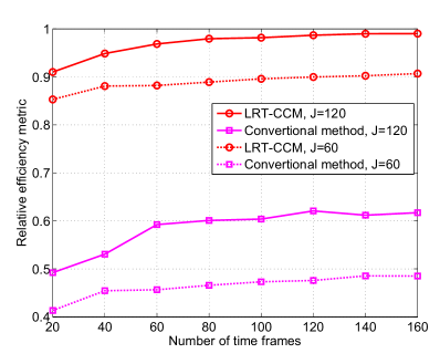
(a) REM

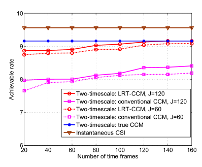
(b) Achievable rate

Figure 3: REMs and achievable rates of respective methods, where we set $\text{SNR}=0$dB, $J=60$ and $J=120$.

Next, we examine the impact of the number of time frames on the estimation and beamforming performance. Fig. 3 plots the performance of respective methods as a function of $T$, where we set SNR to $0$dB, and $J$ is set to $J=60$ and $J=120$, respectively. It can be observed from Fig. 3 that a small value of $T$, say $T=20$ is sufficient to achieve a decent performance for our proposed method. Increasing the number of time frames can lead to better performance for both methods, but the performance improvement is very limited. Since the total number of measurements required for training is $TJ$, this result suggests that our proposed method can provide a reliable CCM estimate using a training overhead as small as $TJ=20\times 60=1200$. Fig. 4 illustrates the effect of the number of time slots on the estimation and beamforming performance of respective methods, where we set $\text{SNR}=0\text{dB}$, and $T$ is set to $T=40$ and $T=100$, respectively. We see that increasing the number of time slots leads to better performance. Nevertheless, a small value of $J$, say, $J=60$, is enough to provide a decent performance for our proposed method. Again, this result demonstrates the ability of the proposed method in providing an accurate CCM using a small amount of training overhead.

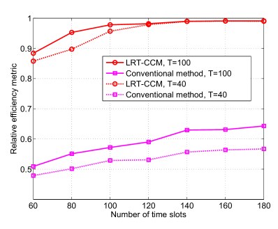
(a) REM

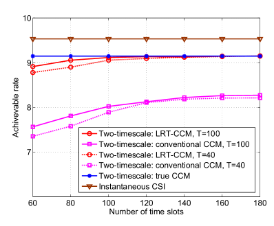
(b) Achievable rate

Figure 4: REMs and achievable rates of respective methods, where we set $\text{SNR}=0$dB, $T=40$ and $T=100$.

VIII Conclusions

In this paper, we considered the CCM estimation for IRS-assisted mmWave communication systems. We exploited the low-rank property and PSD 3-level Toeplitz structure of the CCM and formulated the CCM estimation problem as a convex SDP problem, which was further efficiently solved by an ADMM algorithm. In addition, we analyzed the estimation performance of the proposed solution, as well as the training overhead required to obtain a reliable estimate of the CCM. Lastly, we discussed how to perform the two-timescale beamforming based on the estimated CCM. Simulation results showed that our proposed method can provide a reliable CCM estimate using a small amount of training overhead.

Appendix A Proof of Theorem 1

Based on the definition, the trace of a PSD matrix is equivalent to its nuclear norm. For simplicity, we consider the following equivalent form of (38):

$$\boldsymbol{\hat{R}}_{h}=\arg\min_{\boldsymbol{{R}}_{h}}\frac{1}{2}\left\|\boldsymbol{\hat{R}}_{y}-\boldsymbol{W}\boldsymbol{{R}}_{h}\boldsymbol{W}^{H}\right\|_{F}^{2}+\lambda\|\boldsymbol{{R}}_{h}\|_{*}$$ (83)

where $\|\cdot\|_{*}$ denotes the nuclear norm.

In order to prove Theorem 1, we first introduce the following theorem [26].

Theorem 2

For the convex optimization problem

$$\widehat{\boldsymbol{\Theta}}_{\lambda_{n}}\in\arg\min_{\boldsymbol{\Theta}}\left\{\mathcal{L}\left(\boldsymbol{\Theta}\right)+\lambda_{n}\mathcal{R}(\boldsymbol{\Theta})\right\}$$ (84)

where $\lambda_{n}>0$ is a user-defined regularization parameter and $\mathcal{R}(\cdot)$ is a norm. Suppose that $\mathcal{L}$ is a convex and differentiable function, and consider any optimal solution $\widehat{\boldsymbol{\Theta}}$ to the aforementioned optimization problem with a strictly positive regularization parameter satisfying

$$\lambda_{n}\geq 2\mathcal{R}^{*}(\nabla\mathcal{L}\left(\boldsymbol{\Theta}^{*}\right))$$ (85)

where $\mathcal{R}^{*}(\cdot)$ is the dual norm of $\mathcal{R}(\cdot)$ and $\boldsymbol{\Theta}^{*}$ is the unknown true value. Denote $\mathcal{M}\subseteq\bar{\mathcal{M}}$ as the subspace to capture the constraints specified by the norm-based regularizer and $\bar{\mathcal{M}}^{\perp}$ as the orthogonal complement of space $\bar{\mathcal{M}}$. Then for any pair $\left(\mathcal{M},\bar{\mathcal{M}}^{\perp}\right)$ over which $\mathcal{R}$ is decomposable, the error $\boldsymbol{\Delta}=\widehat{\boldsymbol{\Theta}}_{\lambda_{n}}-\boldsymbol{\Theta}^{*}$ belongs to the set

$$\mathbb{C}\left(\mathcal{M},\bar{\mathcal{M}}^{\perp};\boldsymbol{\Theta}^{*}\right)$$

$$\quad\triangleq\left\{\boldsymbol{\Delta}|\mathcal{R}\left(\boldsymbol{\Delta}_{\bar{\mathcal{M}}^{\perp}}\right)\right.\left.\leq 3\mathcal{R}\left(\boldsymbol{\Delta}_{\bar{\mathcal{M}}}\right)+4\mathcal{R}\left(\boldsymbol{\Theta}_{\mathcal{M}^{\perp}}^{*}\right)\right\}$$ (86)

where $\mathcal{M}^{\perp}$ is the orthogonal complement of the space $\mathcal{M}$. In (86) $\boldsymbol{\Delta}_{\bar{\mathcal{M}}}$ denotes the projection of $\boldsymbol{\Delta}$ onto the subspace $\bar{\mathcal{M}}$, which is defined as

$$\boldsymbol{\Delta}_{\bar{\mathcal{M}}}=\arg\min_{\boldsymbol{\Delta}_{1}\in\bar{\mathcal{M}}}\|\boldsymbol{\Delta}-\boldsymbol{\Delta}_{1}\|_{F}^{2}$$ (87)

${\boldsymbol{\Delta}}_{\bar{\mathcal{M}}^{\perp}}$ and $\boldsymbol{\Theta}_{\mathcal{M}^{\perp}}^{*}$ can be similarly defined (and hence we omit them here). Specifically, $\mathcal{R}\left(\boldsymbol{\Theta}_{\mathcal{M}^{\perp}}^{*}\right)=0$ when $\boldsymbol{\Theta}\in\mathcal{M}$, and under such a circumstance (86) turns to be

$$\mathbb{C}\left(\mathcal{M},\bar{\mathcal{M}}^{\perp};\boldsymbol{\Theta}^{*}\right)\triangleq\left\{\boldsymbol{\Delta}|\mathcal{R}\left(\boldsymbol{\Delta}_{\bar{\mathcal{M}}^{\perp}}\right)\right.\left.\leq 3\mathcal{R}\left(\boldsymbol{\Delta}_{\bar{\mathcal{M}}}\right)\right\}$$ (88)

Proof:

See [26]. ∎

Theorem 2 implies that with a proper regularization parameter and $\boldsymbol{\Theta}\in\mathcal{M}$, the estimation error of the problem (84) satisfies (88). We know that $\text{rank}(\boldsymbol{R}_{h})=r$ and the SVD of $\boldsymbol{R}_{h}$ is given as $\boldsymbol{R}_{h}=\boldsymbol{U}\boldsymbol{\Sigma}\boldsymbol{V}^{H}$. Let $\text{row}(\boldsymbol{R}_{h})$ and $\text{col}(\boldsymbol{R}_{h})$ denote the row and column space of $\boldsymbol{R}_{h}$ respectively, and meanwhile let $\boldsymbol{U}^{r}$ and $\boldsymbol{V}^{r}$ be the first $r$ columns of $\boldsymbol{U}$ and $\boldsymbol{V}$. We now can define the subspace $\mathcal{M}$ and $\bar{\mathcal{M}}^{\perp}$ as

$$\mathcal{M}=\bar{\mathcal{M}}\triangleq\{\boldsymbol{R}|\text{row}(\boldsymbol{R})=\boldsymbol{V}^{r},\text{col}(\boldsymbol{R})=\boldsymbol{U}^{r}\}$$ (89)

$$\bar{\mathcal{M}}^{\perp}\triangleq\{\boldsymbol{R}|\text{row}(\boldsymbol{R})={(\boldsymbol{V}^{r})}^{\perp},\text{col}(\boldsymbol{R})={(\boldsymbol{U}^{r})}^{\perp}\}$$ (90)

Utilizing these defined subspaces, we can conclude that $\boldsymbol{R}_{h}\in\mathcal{M}$, and meanwhile the estimation error of $\boldsymbol{R}_{h}$, i.e., $\boldsymbol{\Delta}\triangleq\boldsymbol{\hat{R}}_{h}-\boldsymbol{R}_{h}$, can be decomposed into two parts, i.e.,

$$\boldsymbol{\Delta}=\boldsymbol{\Delta}_{1}+\boldsymbol{\Delta}_{2}$$ (91)

with $\text{rank}(\boldsymbol{\Delta}_{1})=r$, $\boldsymbol{\Delta}_{1}\in\mathcal{M}$ and $\boldsymbol{\Delta}_{2}\in\bar{\mathcal{M}}^{\perp}$.

In our problem, $\mathcal{L}\left(\boldsymbol{\Theta}\right)=\frac{1}{2}\|\boldsymbol{\hat{R}}_{y}-\boldsymbol{W}\boldsymbol{R}_{h}\boldsymbol{W}^{H}\|_{F}^{2}$. Therefore, we have

$$\nabla\mathcal{L}\left(\boldsymbol{R}_{h}\right)=\frac{1}{2}\left[\boldsymbol{W}^{H}(\boldsymbol{W}\boldsymbol{R}_{h}\boldsymbol{W}^{H}-\boldsymbol{\hat{R}}_{y})\boldsymbol{W}\right]^{T}$$ (92)

In addition, it is clear that the dual norm of the nuclear norm is the spectral norm. Therefore, if the regularization parameter $\lambda$ satisfies

$$\lambda\geq 2\mathcal{R}^{*}(\nabla\mathcal{L}\left(\boldsymbol{R}_{h}\right)) =\|\boldsymbol{W}^{H}(\boldsymbol{\hat{R}}_{y}-\boldsymbol{W}\boldsymbol{R}_{h}\boldsymbol{W}^{H})\boldsymbol{W}\|_{2}$$

$$=\|\boldsymbol{W}^{H}(\boldsymbol{\hat{R}}_{y}-\boldsymbol{R}_{y})\boldsymbol{W}\|_{2}$$ (93)

then the estimation error, based on Theorem 2, belongs to the set

$$\boldsymbol{\Delta} \triangleq\boldsymbol{\hat{R}}_{h}-\boldsymbol{R}_{h}=\mathbb{T}_{3}(\hat{\boldsymbol{V}})-\mathbb{T}_{3}({\boldsymbol{V}})=\mathbb{T}_{3}(\hat{\boldsymbol{V}}-{\boldsymbol{V}})$$

$$\in\{\boldsymbol{\Delta}|\boldsymbol{\Delta}=\boldsymbol{\Delta}_{1}+\boldsymbol{\Delta}_{2},\ \|\boldsymbol{\Delta}_{2}\|_{*}\leq 3\|\boldsymbol{\Delta}_{1}\|_{*}\}$$ (94)

From (93), we can see that the choice of $\lambda$ depends on the value of $\|\boldsymbol{W}^{H}(\boldsymbol{\hat{R}}_{y}-\boldsymbol{R}_{y})\boldsymbol{W}\|_{2}$. The following lemma provides an upper bound on $\|\boldsymbol{W}^{H}(\boldsymbol{\hat{R}}_{y}-\boldsymbol{R}_{y})\boldsymbol{W}\|_{2}$.

Lemma 1

Given $T$ observation samples $\{\boldsymbol{y}_{t}\}_{t=1}^{T}$, $\boldsymbol{\hat{R}}_{y}$ is obtained via $\frac{1}{T}\sum_{t=1}^{T}\boldsymbol{y}_{t}\boldsymbol{y}_{t}^{H}$. Then with probability at least $1-4T^{-1}$, we have

$$\|\boldsymbol{W}^{H}(\boldsymbol{\hat{R}}_{y}-\boldsymbol{R}_{y})\boldsymbol{W}\|_{2}$$

$$\qquad\qquad\leq\delta\triangleq c\|\boldsymbol{W}\|_{F}^{2}\|\boldsymbol{R}_{y}\|_{2}\text{max}\{\sqrt{\tilde{\delta}},\tilde{\delta}\}$$ (95)

where $\tilde{\delta}$ is given in (66).

Proof:

See Appendix B. ∎

Since $\boldsymbol{\hat{R}}_{h}$ is the optimal solution to (83), we have

$$\frac{1}{2}\left\|\boldsymbol{\hat{R}}_{y}-\boldsymbol{W}\boldsymbol{\hat{R}}_{h}\boldsymbol{W}^{H}\right\|_{F}^{2}+\lambda\|\boldsymbol{\hat{R}}_{h}\|_{*}$$

$$\qquad\leq\frac{1}{2}\left\|\boldsymbol{\hat{R}}_{y}-\boldsymbol{W}{\boldsymbol{R}}_{h}\boldsymbol{W}^{H}\right\|_{F}^{2}+\lambda\|{\boldsymbol{R}}_{h}\|_{*}$$ (96)

which can be converted to

$$\left\|\boldsymbol{\hat{R}}_{y}-\boldsymbol{W}\boldsymbol{\hat{R}}_{h}\boldsymbol{W}^{H}\right\|_{F}^{2} -\left\|\boldsymbol{\hat{R}}_{y}-\boldsymbol{W}{\boldsymbol{R}}_{h}\boldsymbol{W}^{H}\right\|_{F}^{2}$$

$$\qquad\leq 2\lambda\Big{(}\|{\boldsymbol{R}}_{h}\|_{*}-\|\boldsymbol{\hat{R}}_{h}\|_{*}\Big{)}$$ (97)

Recalling $\boldsymbol{\Delta}=\boldsymbol{\hat{R}}_{h}-\boldsymbol{R}_{h}$, the left side of (97) can be further expressed as

$$\left\|\boldsymbol{\hat{R}}_{y}-\boldsymbol{W}\hat{\boldsymbol{R}}_{h}\boldsymbol{W}^{H}\right\|_{F}^{2}-\left\|\boldsymbol{\hat{R}}_{y}-\boldsymbol{W}{\boldsymbol{R}}_{h}\boldsymbol{W}^{H}\right\|_{F}^{2}$$

$$=\left\|\boldsymbol{\hat{R}}_{y}-\boldsymbol{W}({\boldsymbol{R}}_{h}+\boldsymbol{\Delta})\boldsymbol{W}^{H}\right\|_{F}^{2}-\left\|\boldsymbol{\hat{R}}_{y}-\boldsymbol{W}{\boldsymbol{R}}_{h}\boldsymbol{W}^{H}\right\|_{F}^{2}$$

$$=2\langle-\boldsymbol{\hat{R}}_{y}+\boldsymbol{W}{\boldsymbol{R}}_{h}\boldsymbol{W}^{H},\boldsymbol{W}\Delta\boldsymbol{W}^{H}\rangle+\left\|\boldsymbol{W}\boldsymbol{\Delta}\boldsymbol{W}^{H}\right\|_{F}^{2}$$

$$=2\langle\boldsymbol{W}^{H}(-\boldsymbol{\hat{R}}_{y}+\boldsymbol{W}{\boldsymbol{R}}_{h}\boldsymbol{W}^{H})\boldsymbol{W},\boldsymbol{\Delta}\rangle+\left\|\boldsymbol{W}\boldsymbol{\Delta}\boldsymbol{W}^{H}\right\|_{F}^{2}$$ (98)

Substituting (98) into (97), we have

$$\left\|\boldsymbol{W}\boldsymbol{\Delta}\boldsymbol{W}^{H}\right\|_{F}^{2}$$

$$\leq 2\langle\boldsymbol{W}^{H}(\boldsymbol{\hat{R}}_{y}-\boldsymbol{W}{\boldsymbol{R}}_{h}\boldsymbol{W}^{H})\boldsymbol{W},\boldsymbol{\Delta}\rangle+2\lambda\Big{(}\|{\boldsymbol{R}}_{h}\|_{*}-\|\hat{\boldsymbol{R}}_{h}\|_{*}\Big{)}$$

$$\overset{(a)}{\leq}2\|\boldsymbol{W}^{H}(\boldsymbol{\hat{R}}_{y}-\boldsymbol{W}{\boldsymbol{R}}_{h}\boldsymbol{W}^{H})\boldsymbol{W}\|\|\boldsymbol{\Delta}\|_{*}$$

$$\qquad\qquad\qquad\qquad\qquad+2\lambda\Big{(}\|\boldsymbol{\hat{R}}_{h}+\boldsymbol{\Delta}\|_{*}-\|\boldsymbol{\hat{R}}_{h}\|_{*}\Big{)}$$

$$\overset{(b)}{\leq}2\|\boldsymbol{W}^{H}(\boldsymbol{\hat{R}}_{y}-\boldsymbol{W}{\boldsymbol{R}}_{h}\boldsymbol{W}^{H})\boldsymbol{W}\|\|\boldsymbol{\Delta}\|_{*}+2\lambda\|\boldsymbol{\Delta}\|_{*}$$

$$\overset{(c)}{\leq}4\lambda\left\|\boldsymbol{\Delta}\right\|_{*}$$ (99)

where $(a)$ follows from Holder’s inequality, $(b)$ comes from the triangle inequality, and $(c)$ follows from the assumption $\lambda\geq\delta$. Furthermore, we have

$$\left\|\boldsymbol{\Delta}\right\|_{*} =\left\|\boldsymbol{\Delta}_{1}+\boldsymbol{\Delta}_{2}\right\|_{*}\leq\left\|\boldsymbol{\Delta}_{1}\right\|_{*}+\left\|\boldsymbol{\Delta}_{2}\right\|_{*}$$

$$\overset{(a)}{\leq}\left\|\boldsymbol{\Delta}_{1}\right\|_{*}+3\left\|\boldsymbol{\Delta}_{1}\right\|_{*}$$

$$\overset{(b)}{\leq}4\sqrt{r}\|\boldsymbol{\Delta}_{1}\|_{F}$$

$$\leq 4\sqrt{r}\left\|\boldsymbol{\Delta}\right\|_{F}=4\sqrt{r}\left\|\mathbb{T}_{3}(\hat{\boldsymbol{V}}-\boldsymbol{V})\right\|_{F}$$

$$\leq 4\sqrt{rNM}\|\hat{\boldsymbol{V}}-\boldsymbol{V}\|_{F}$$ (100)

where $(a)$ follows from (94), and $(b)$ is a result of the relationship between the nuclear norm and F-norm of a rank-$r$ matrix. Putting (99) and (100) together results in

$$\left\|\boldsymbol{W}\boldsymbol{\Delta}\boldsymbol{W}^{H}\right\|_{F}^{2}\leq 16\lambda\sqrt{rNM}\|\hat{\boldsymbol{V}}-\boldsymbol{V}\|_{F}$$ (101)

Furthermore, we utilize the following lemma to find a lower bound of $\left\|\boldsymbol{W}\boldsymbol{\Delta}\boldsymbol{W}^{H}\right\|_{F}^{2}$.

Lemma 2

Consider a 3-level Toeplitz matrix $\mathbb{T}_{3}(\boldsymbol{{X}})$ with $\boldsymbol{X}\in\mathbb{C}^{(2I_{1}-1)\times(2I_{2}-1)\times(2I_{3}-1)}$ and the matrix $\boldsymbol{W}\in\mathbb{C}^{I^{2}\times I_{1}I_{2}I_{3}}$. If

$$I\geq\sqrt{(2I_{1}-1)(2I_{2}-1)(2I_{3}-1)}$$ (102)

then with high probability there exists a full-column rank transforming matrix $\boldsymbol{\check{W}}$ of $\boldsymbol{W}$ such that

$$\|\boldsymbol{W}\mathbb{T}_{3}(\boldsymbol{{X}})\boldsymbol{W}^{H}\|_{F}^{2}\geq\sigma_{\text{min}}^{2}(\boldsymbol{\check{W}})\|\boldsymbol{{X}}\|_{F}^{2}$$ (103)

where $\sigma_{\text{min}}(\boldsymbol{\check{W}})$ is the smallest singular value of $\boldsymbol{\check{W}}$.

Proof:

See Appendix C. ∎

Since we have

$$J\geq u\triangleq\sqrt{(2N-1)(2M_{v}-1)(2M_{h}-1)}$$ (104)

and meanwhile $\boldsymbol{\Delta}=\mathbb{T}_{3}(\boldsymbol{\hat{V}}-\boldsymbol{V})$ is a 3-level Toeplitz matrix, based on Lemma 2, we know that, with high probability the following holds

$$\|\boldsymbol{W}\boldsymbol{\Delta}\boldsymbol{W}^{H}\|_{F}^{2}\geq\sigma_{\text{min}}^{2}(\boldsymbol{\check{W}})\|\hat{\boldsymbol{V}}-\boldsymbol{V}\|_{F}^{2}$$ (105)

where $\boldsymbol{\check{W}}$ is the transforming matrix of $\boldsymbol{W}$. Substituting (105) into (101) leads to

$$\|\boldsymbol{\hat{V}}-\boldsymbol{V}\|_{F}\leq\frac{16\lambda\sqrt{rNM}}{\sigma_{\text{min}}^{2}(\boldsymbol{\check{W}})}$$ (106)

As a result, the average per-entry RMSE is given by

$$\frac{1}{u}\|\boldsymbol{\hat{V}}-\boldsymbol{V}\|_{F}\leq\frac{16\lambda\sqrt{r}}{\sigma^{2}_{\text{min}}(\boldsymbol{\check{W}})}\frac{\sqrt{NM}}{u}$$ (107)

which completes the proof.

Appendix B Proof of Lemma 1

The received signal $\boldsymbol{y}_{t}$ follows a complex Gaussian $\mathbb{CN}(0,\boldsymbol{R}_{y})$. Therefore, according to Theorem 2.2 in [32] we know that, with probability at least $1-4T^{-1}$, the following inequality holds

$$\|\boldsymbol{\hat{R}}_{y}-\boldsymbol{R}_{y}\|_{2}\leq c\|\boldsymbol{R}_{y}\|_{2}\text{max}\{\sqrt{\tilde{\delta}},\tilde{\delta}\}$$ (108)

where $c$ is a constant. Furthermore, we have

$$\|\boldsymbol{W}^{H}(\boldsymbol{\hat{R}}_{y}-\boldsymbol{R}_{y})\boldsymbol{W}\|_{2}$$

$$\overset{(a)}{\leq}\|\boldsymbol{W}^{H}(\boldsymbol{\hat{R}}_{y}-\boldsymbol{R}_{y})\boldsymbol{W}\|_{F}$$

$$\overset{(b)}{\leq}\|\boldsymbol{W}\|_{F}^{2}\|(\boldsymbol{\hat{R}}_{y}-\boldsymbol{R}_{y})\|_{2}$$

$$\leq c\|\boldsymbol{W}\|_{F}^{2}\|\boldsymbol{R}_{y}\|_{2}\text{max}\{\sqrt{\tilde{\delta}},\tilde{\delta}\}$$ (109)

where $(a)$ follows from the fact that $\|\boldsymbol{A}\|_{2}\leq\|\boldsymbol{A}\|_{F}$ and $(b)$ follows from $\|\boldsymbol{A}\boldsymbol{B}\|_{F}\leq\|\boldsymbol{A}\|_{2}\|\boldsymbol{B}\|_{F}$.

Appendix C Proof of Lemma 2

According to the Kronecker product property, we have

$$\text{vec}(\boldsymbol{W}\mathbb{T}_{3}(\boldsymbol{{X}})\boldsymbol{W}^{H}) =(\boldsymbol{W}^{*}\otimes\boldsymbol{W})\text{vec}(\mathbb{T}_{3}(\boldsymbol{X}))$$ (110)

Since $\mathbb{T}_{3}(\boldsymbol{X})$ is a 3-level Toeplitz matrix, we can express (110) as

$$(\boldsymbol{W}^{*}\otimes\boldsymbol{W})\text{vec}(\mathbb{T}_{3}(\boldsymbol{{X}}))=\boldsymbol{\check{W}}\boldsymbol{x}$$ (111)

where $\boldsymbol{x}=\text{vec}(\boldsymbol{X})$ and $\boldsymbol{\check{W}}\in\mathbb{C}^{I^{2}\times(2I_{1}-1)(2I_{2}-1)(2I_{3}-1)}$ is constructed by combining those columns in $\boldsymbol{W}^{*}\otimes\boldsymbol{W}$ which correspond to the same element in $\mathbb{T}_{3}(\boldsymbol{X})$. Furthermore, $\boldsymbol{\check{W}}$ is a full-column rank matrix with high probability due to the fact that $\boldsymbol{W}$ is a random matrix and the condition (102) holds. Since $\boldsymbol{\check{W}}$ is a full-column rank matrix, we have

$$\|\boldsymbol{\check{W}}\boldsymbol{x}\|_{2}^{2}\geq\sigma_{\text{min}}^{2}(\boldsymbol{\check{W}})\|\boldsymbol{x}\|_{2}^{2}\equiv\sigma_{\text{min}}^{2}(\boldsymbol{\check{W}})\|\boldsymbol{X}\|_{F}^{2}$$ (112)

Due to that fact that $\|\boldsymbol{A}\|_{F}^{2}=\|\text{vec}(\boldsymbol{A})\|_{2}^{2}$ for an arbitrary matrix $\boldsymbol{A}$, we have

$$\|\boldsymbol{W}\mathbb{T}_{3}(\boldsymbol{X})\boldsymbol{W}^{H}\|_{F}^{2}=\|\boldsymbol{\check{W}}\boldsymbol{x}\|_{2}^{2}\geq\sigma_{\text{min}}^{2}(\boldsymbol{\check{W}})\|\boldsymbol{X}\|_{F}^{2}$$ (113)

which completes the proof.

Appendix D Multi-level Toeplitz Matrix

Given a $d$-order tensor $\boldsymbol{{U}}_{d}\in\mathbb{C}^{(2k_{d}-1)\times\cdots\times(2k_{1}-1)}$, its corresponding $d$-level Toeplitz matrix $\mathbb{T}_{d}(\boldsymbol{{U}}_{d})$ is defined in the following recursive manner. For $d=1$, $\boldsymbol{{U}}_{d}$ is essentially a vector $\boldsymbol{u}_{1}\in\mathbb{C}^{2k_{1}-1}$, in which case $\mathbb{T}_{1}(\boldsymbol{u}_{1})$ is given by

$$\mathbb{T}_{1}(\boldsymbol{u}_{1})=\begin{bmatrix}\boldsymbol{u}_{1}(0)&\boldsymbol{u}_{1}(1)&\cdots&\boldsymbol{u}_{1}(k_{1}-1)\\ \boldsymbol{u}_{1}(-1)&\boldsymbol{u}_{1}(0)&\cdots&\boldsymbol{u}_{1}(k_{1}-2)\\ \vdots&\vdots&\ddots&\vdots\\ \boldsymbol{u}_{1}(1-k_{1})&\boldsymbol{u}_{1}(2-k_{1})&\cdots&\boldsymbol{u}_{1}(0)\\ \end{bmatrix}$$ (114)

For $d\geq 2$, Let $\boldsymbol{{U}}_{d-1}(i)=\boldsymbol{{U}}_{d}(i,:,\cdots,:)$ with $i$ from $-k_{d}+1$ to $k_{d}-1$, and denote $\mathbb{T}_{d-1}(\boldsymbol{{U}}_{d-1}(i))$ as $\boldsymbol{D}(i)$. We have

$$\mathbb{T}_{d}(\boldsymbol{{U}}_{d})=\begin{bmatrix}\boldsymbol{D}(0)&\boldsymbol{D}(1)&\cdots&\boldsymbol{D}(k_{d}-1)\\ \boldsymbol{D}(-1)&\boldsymbol{D}(0)&\cdots&\boldsymbol{D}(k_{d}-2)\\ \vdots&\vdots&\ddots&\vdots\\ \boldsymbol{D}(1-k_{d})&\boldsymbol{D}(2-k_{d})&\cdots&\boldsymbol{D}(0)\\ \end{bmatrix}$$ (115)

References

- [1] S. Rangan, T. S. Rappaport, and E. Erkip, “Millimeter-wave cellular wireless networks: potentials and challenges,” Proceedings of the IEEE, vol. 102, no. 3, pp. 366–385, 2014.
- [2] P. Wang, J. Fang, X. Yuan, Z. Chen, and H. Li, “Intelligent reflecting surface-assisted millimeter wave communications: Joint active and passive precoding design,” IEEE Transactions on Vehicular Technology, vol. 69, no. 12, pp. 14 960–14 973, 2020.
- [3] Q. Wu and R. Zhang, “Intelligent reflecting surface enhanced wireless network via joint active and passive beamforming,” IEEE Transactions on Wireless Communications, vol. 18, no. 11, pp. 5394–5409, 2019.
- [4] B. Zheng, C. You, W. Mei, and R. Zhang, “A survey on channel estimation and practical passive beamforming design for intelligent reflecting surface aided wireless communications,” IEEE Communications Surveys & Tutorials, 2022.
- [5] P. Wang, J. Fang, H. Duan, and H. Li, “Compressed channel estimation for intelligent reflecting surface-assisted millimeter wave systems,” IEEE Signal Processing Letters, vol. 27, pp. 905–909, 2020.
- [6] S. Liu, Z. Gao, J. Zhang, M. Di Renzo, and M.-S. Alouini, “Deep denoising neural network assisted compressive channel estimation for mmwave intelligent reflecting surfaces,” IEEE Transactions on Vehicular Technology, vol. 69, no. 8, pp. 9223–9228, 2020.
- [7] X. Wei, D. Shen, and L. Dai, “Channel estimation for RIS assisted wireless communications–part II: An improved solution based on double-structured sparsity,” IEEE Communications Letters, vol. 25, no. 5, pp. 1403–1407, 2021.
- [8] W. Wang and W. Zhang, “Joint beam training and positioning for intelligent reflecting surfaces assisted millimeter wave communications,” IEEE Transactions on Wireless Communications, vol. 20, no. 10, pp. 6282–6297, 2021.
- [9] P. Wang, J. Fang, W. Zhang, and H. Li, “Fast beam training and alignment for IRS-assisted millimeter wave/terahertz systems,” IEEE Transactions on Wireless Communications, vol. 21, no. 4, pp. 2710–2724, 2022.
- [10] P. Wang, J. Fang, W. Zhang, Z. Chen, H. Li, and W. Zhang, “Beam training and alignment for RIS-assisted millimeter wave systems: State of the art and beyond,” IEEE Wireless Communications, to appear.
- [11] Y. Lin, S. Jin, M. Matthaiou, and X. You, “Channel estimation and user localization for IRS-assisted MIMO-OFDM systems,” IEEE Transactions on Wireless Communications, 2021.
- [12] G. T. de Araújo, A. L. De Almeida, and R. Boyer, “Channel estimation for intelligent reflecting surface assisted MIMO systems: A tensor modeling approach,” IEEE Journal of Selected Topics in Signal Processing, vol. 15, no. 3, pp. 789–802, 2021.
- [13] X. Zheng, P. Wang, J. Fang, and H. Li, “Compressed channel estimation for IRS-assisted millimeter wave OFDM systems: A low-rank tensor decomposition-based approach,” IEEE Wireless Communications Letters, pp. 1–1, 2022.
- [14] F. Yang, J.-B. Wang, H. Zhang, C. Chang, and J. Cheng, “Intelligent reflecting surface-assisted mmwave communication exploiting statistical CSI,” in 2020 IEEE International Conference on Communications (ICC). Dublin, Ireland, 2020, pp. 1–6.
- [15] X. Hu, F. Gao, C. Zhong, X. Chen, Y. Zhang, and Z. Zhang, “An angle domain design framework for intelligent reflecting surface systems,” in 2020 IEEE Global Communications Conference (GLOBECOM). Taipei, Taiwan, 2020, pp. 1–6.
- [16] X. Hu, J. Wang, and C. Zhong, “Statistical CSI based design for intelligent reflecting surface assisted MISO systems,” Science China Information Sciences, vol. 63, no. 12, pp. 1–10, 2020.
- [17] M.-M. Zhao, Q. Wu, M.-J. Zhao, and R. Zhang, “Intelligent reflecting surface enhanced wireless networks: Two-timescale beamforming optimization,” IEEE Transactions on Wireless Communications, vol. 20, no. 1, pp. 2–17, 2021.
- [18] X. Gan, C. Zhong, C. Huang, and Z. Zhang, “RIS-assisted multi-user MISO communications exploiting statistical CSI,” IEEE Transactions on Communications, vol. 69, no. 10, pp. 6781–6792, 2021.
- [19] S. Park and R. W. Heath, “Spatial channel covariance estimation for the hybrid MIMO architecture: A compressive sensing-based approach,” IEEE Transactions on Wireless Communications, vol. 17, no. 12, pp. 8047–8062, 2018.
- [20] S. Park, A. Ali, N. González-Prelcic, and R. W. Heath, “Spatial channel covariance estimation for hybrid architectures based on tensor decompositions,” IEEE Transactions on Wireless Communications, vol. 19, no. 2, pp. 1084–1097, 2019.
- [21] Y. Wang, Y. Zhang, Z. Tian, G. Leus, and G. Zhang, “Super-resolution channel estimation for arbitrary arrays in hybrid millimeter-wave massive MIMO systems,” IEEE Journal of Selected Topics in Signal Processing, vol. 13, no. 5, pp. 947–960, 2019.
- [22] O. El Ayach, S. Rajagopal, S. Abu-Surra, Z. Pi, and R. W. Heath, “Spatially sparse precoding in millimeter wave MIMO systems,” IEEE Transactions on Wireless Communications, vol. 13, no. 3, pp. 1499–1513, 2014.
- [23] I. Viering, H. Hofstetter, and W. Utschick, “Spatial long-term variations in urban, rural and indoor environments,” in Proceedings of the 5th Metting COST. Lisbon, Pirtugal, 2002.
- [24] A. Alkhateeb, O. El Ayach, G. Leus, and R. W. Heath, “Channel estimation and hybrid precoding for millimeter wave cellular systems,” IEEE Journal of Selected Topics in Signal Processing, vol. 8, no. 5, pp. 831–846, 2014.
- [25] Y. Li and Y. Chi, “Off-the-grid line spectrum denoising and estimation with multiple measurement vectors,” IEEE Transactions on Signal Processing, vol. 64, no. 5, pp. 1257–1269, 2015.
- [26] S. N. Negahban, P. Ravikumar, M. J. Wainwright, and B. Yu, “A unified framework for high-dimensional analysis of -estimators with decomposable regularizers,” Statistical Science, vol. 27, no. 4, pp. 538–557, 2012.
- [27] A. M.-C. So, J. Zhang, and Y. Ye, “On approximating complex quadratic optimization problems via semidefinite programming relaxations,” Mathematical Programming, vol. 110, no. 1, pp. 93–110, 2007.
- [28] S. Haghighatshoar and G. Caire, “Massive MIMO channel subspace estimation from low-dimensional projections,” IEEE Transactions on Signal Processing, vol. 65, no. 2, pp. 303–318, 2016.
- [29] S. Park, J. Park, A. Yazdan, and R. W. Heath, “Exploiting spatial channel covariance for hybrid precoding in massive MIMO systems,” IEEE Transactions on Signal Processing, vol. 65, no. 14, pp. 3818–3832, 2017.
- [30] C. K. Anjinappa, A. C. Gürbüz, Y. Yapıcı, and I. Güvenç, “Off-grid aware channel and covariance estimation in mmwave networks,” IEEE Transactions on Communications, vol. 68, no. 6, pp. 3908–3921, 2020.
- [31] X. Yu, D. Xu, and R. Schober, “MISO wireless communication systems via intelligent reflecting surfaces,” in 2019 IEEE/CIC International Conference on Communications in China (ICCC). Changchun, China, 2019, pp. 735–740.
- [32] F. Bunea and L. Xiao, “On the sample covariance matrix estimator of reduced effective rank population matrices, with applications to fPCA,” Bernoulli, vol. 21, no. 2, pp. 1200–1230, 2015.