Classification of KPI lumps

Abstract

A large family of nonsingular rational solutions of the Kadomtsev-Petviashvili (KP) I equation are investigated. These solutions are constructed via the Gramian method and are identified as points in a complex Grassmannian. Each solution is a traveling wave moving with a uniform background velocity but have multiple peaks which evolve at a slower time scale in the co-moving frame. For large times, these peaks separate and form well-defined wave patterns in the $xy$-plane. The pattern formation are described by the roots of well-known polynomials arising in the study of rational solutions of Painlevé II and IV equations. This family of solutions are shown to be described by the classical Schur functions associated with partitions of integers and irreducible representations of the symmetric group of $N$ objects. It is then shown that there exists a one-to-one correspondence between the KPI rational solutions considered in this article and partitions of a positive integer $N$.

1 Introduction

An important example of nonlinear wave equations in $(2+1)$-dimensions is the Kadomtsev-Petviashvili (KP) equation, which is dispersive equation describing the propagation of small amplitude, long wavelength, uni-directional waves with small transverse variation. It was originally proposed by Kadomtsev and Petviashvili [24] to study ion-acoustic waves of small amplitude propagating in plasmas. The KP equation has many physical applications and arises in such diverse fields as plasma physics [22, 28], fluid dynamics [4, 1, 27], nonlinear optics  [39, 8] and ferromagnetic media  [44]. It is also an exactly solvable nonlinear equation with remarkably rich mathematical structure documented in many research monographs (see e.g. [34, 2, 22, 21, 27]).

There are two mathematically distinct versions of the KP equation, referred to as KPI and KPII. This article is concerned with the KPI equation which can be expressed as

$$(4u_{t}+6uu_{x}+u_{xxx})_{x}=3u_{yy}.$$ (1.1)

Here $u=u(x,y,t)$ represents the normalized wave amplitude at the point $(x,y)$ in the $xy$-plane for fixed time $t$, and the subscripts denote partial derivatives. The KPII equation is (1.1) with $-3u_{yy}$ in the right hand side. From the water wave theory perspective, KPI corresponds to large surface tension while KPII arises in the small surface tension limit of the multiple-scale asymptotics [4, 1].

The KPI equation admits large classes of exact rational solutions known as lumps which are localized in the $xy$-plane and are non-singular for all $t$. The simplest type of rational solutions was first discovered analytically by employing the dressing method [30] and subsequently via the Hirota method [42]. These solutions consist of $N$ local maxima (peaks) traveling with distinct velocities and their trajectories remain unchanged before and after interaction. These solutions are often referred to as simple lumps in contrast to yet another class of KPI rational solutions arise as bound states formed by fusing the simple lump solutions in a certain manner. These are called the multi-lump solutions which were originally found in [23] by algebraic techniques and further investigated by several authors [37, 20, 3]. The multi-lump solution is an ensemble of a finite number of localized structures (or peaks) interacting in a non-trivial manner unlike the $N$-simple lump solution. The peaks move with the same center-of-mass velocity but undergo anomalous scattering with a non-zero deflection angle after collision. Furthermore, the peak amplitudes evolve in time and reaches a constant asymptotic value which equals that of the simple $1$-lump peak. Both simple and multi-lump rational solutions of the KPI equation are rational potentials associated with the time-dependent Schrödinger equation, and were studied via inverse scattering method [5, 45].

In this article, a large family of rational solutions of KPI described above as multi-lump solutions, are investigated. These solutions constructed here via the Gramian method which expresses the solutions in terms of the determinant (Gramian) of a Gram matrix. The entries of the Gram matrix are constructed out of the inner products of $n$ linearly independent complex vectors which spans a $n$-dimensional subspace which represents a non-degenerate point $V_{P}$ in a complex Grassmannian. Then the Gramian which is the $\tau$-function of the associated KPI solution is the norm of the complex $n$-form obtained as the image of $V_{P}$ via the Plücker embedding of the Grassmannian. It is shown in this paper that this geometric construction leads immediately to a positive definite polynomial form of the $\tau$-function for all $(x,y,t)\in\mathbb{R}^{3}$ so that the resulting KPI rational solution is nonsingular in the $xy$-plane for all $t$ and decays as $(x^{2}+y^{2})^{-1}$.

The next part of this paper describes how to interpret the multi-lump $\tau$-function as a sum of squares in terms of the classical Schur functions which arises in the theory of symmetric functions. The Schur functions are weighted homogeneous polynomials of degree $N$ in $N$ complex variables with specified weights of each variable, and form a basis of symmetric polynomials over integers. The Schur functions play an important role in the Sato theory of the KP equation [41, 36, 27]. However, the relationship between the multi-lump $\tau$-function and the Schur functions unfolded in this article is new, and forms a key feature of the underlying multi-lump solution structure. The Schur functions then lead to a natural characterization that associates each KPI multi-lump solution to a unique partition $\lambda$ of a given positive integer $N$ that is the degree of the corresponding Schur function. Finally, this last characterization can be utilized to formulate a comprehensive classification of the multi-lump solutions which are thus referred to as the $N$-lump solutions of the KPI equation. This classification is also new and completes the task that was initiated in an earlier comprehensive article [3].

Finally, a detailed study of the long time behavior of the $N$-lump solutions is carried out. Our investigation reveals that (a)  for $|t|\gg 1$, the $N$-lump KPI solutions splits into $N$ distinct peaks which form a rich variety of surface wave patterns in the $xy$-plane; and (b)  the solution in the $O(1)$-neighborhood of each peak is a single $1$-lump solution as $|t|\to\infty$ implying that the $N$-lump solution can be viewed as a superposition of $N$ $1$-lump solutions for large times. The approximate location of the peaks are determined in terms of the zeros of the Yablonskii-Vorob’ev and Wronskian-Hermite (heat) polynomials which also describe certain classes of rational solutions of the Painlevé II and IV equations, respectively. This occurrence is not accidental but is related to the similarity reductions of the KPI $N$-lump solutions although this matter will not be pursued further in this paper. Note that the conclusion in part (a) above is based on an assumption that the non-zero roots of the Wronskian-Hermite polynomials are simple [16]. It is also worth noting that some of the exotic surface patterns of the KPI multi-lumps were observed earlier [20, 3, 19, 14] and particularly, the long time asymptotics has been reported recently [48] after our investigation was complete. However, the treatment presented in this paper is new and different from the earlier works since it utilizes the special property of the Schur functions as characteristics of irreducible representation of the symmetric group $S_{N}$. In fact, this property plays a key role in our long time asymptotic analysis which shows that as a whole, the $N$-lump structure is a traveling wave which moves with a uniform velocity while the internal dynamics of the component lumps takes place at a slower time scale $O(|t|^{1/p})$, where (generically) $p=2$ or $p=3$. In a recent paper [10], we analyzed the lump dynamics for a special class of $N$-lump solutions, and showed the dynamics corresponds to a special reduction of the Calogero-Moser system. We believe that is the case for the general KPI $N$-lumps although we do not pursue the matter in this article.

The paper is structured as follows: Section 2 describes the Gramian construction of the $\tau$-function for the multi-lumps and provides some illustrative examples of some simple multi-lump solutions. A brief overview of the Schur functions and integer partition theory is provided in Section 3, followed by a characterization of the KPI solutions by a partition $\lambda$ of a positive integer $N$, that finally leads to a complete classification of the $N$-lump solutions in terms of integer partitions. The long time behavior of the $N$-lump solutions is described in Section 4 which begins with a brief overview of irreducible characters of the symmetric group $S_{N}$, that is essential for the asymptotic analysis presented. Section 5 contains some concluding remarks including future directions of this continued investigation of KPI lumps.

2 Construction of multi-lump solutions

In this section we describe how to construct a large family of multi-lump solutions via Gramians [21] which arise from the application of the binary Darboux transformation to the KPI equation [32]. The building blocks for these solutions are given by a special type of complex polynomials called the generalized Schur polynomials introduced below.

2.1 Generalized Schur polynomials

Let $k$ be a complex parameter and $\theta:=kx+k^{2}y+k^{3}t+\gamma(k)$ where $(x,y,t)\in\mathbb{R}^{3}$ and $\gamma(k)$ is an arbitrary, differentiable (to all orders) function of $k$. The generalized Schur polynomial $p_{n}(x,y,t,k)$ is then defined via

$$\phi_{n}:=\frac{1}{n!}\partial_{k}^{n}\exp(i\theta)=p_{n}\exp(i\theta)\,.$$ (2.1)

The $p_{n}$ is a polynomial in $n$ variables $\theta_{1},\theta_{2},\cdots,\theta_{n}$ with $\theta_{j}:=i{\textstyle\frac{\partial_{k}^{j}\theta}{j!}}$. However, only the first three variables

$$\theta_{1}=i(x+2ky+3k^{2}t+\gamma_{1}),\quad\theta_{2}=i(y+3kt+\gamma_{2}),\quad\theta_{3}=i(t+\gamma_{3})$$ (2.2)

depend on $(x,y,t)$ while $\theta_{j}=i\gamma_{j}(k)$ for $j>3$ depend only on $k$. For a fixed value of $k$, $\gamma_{j}(k)={\textstyle\frac{\partial_{k}^{j}\gamma(k)}{j!}}$, $j=1,\cdots,n$ are viewed as independent complex parameters which parametrize each polynomial $p_{n}$.

A generating function for the $p_{n}$’s is given by the Taylor series

$$\exp(i\theta(k+h))=\exp(i\theta)\sum_{n=0}^{\infty}p_{n}(k)h^{n}\,,$$ (2.3)

which yields, after expanding $i\theta(k+h)=i\theta(k)+h\theta_{1}+h^{2}\theta_{2}+\cdots$, and comparing with the right hand side, an explicit expression for $p_{n}$, namely

$$p_{n}(\theta_{1},\ldots,\theta_{n})=\sum_{\genfrac{}{}{0.0pt}{}{m_{1},m_{2},\cdots,m_{n}\geq 0}{m_{1}+2m_{2}+\cdots nm_{n}=n}}\prod_{j=1}^{n}\frac{\theta_{j}^{m_{j}}}{m_{j}!}\,.$$ (2.4)

The first few generalized Schur polynomials are given by

$$p_{0}=1,\quad p_{1}=\theta_{1},\quad p_{2}={\textstyle\frac{1}{2}}\theta_{1}^{2}+\theta_{2}\quad p_{3}={\textstyle\frac{1}{3!}}\theta_{1}^{3}+\theta_{1}\theta_{2}+\theta_{3}\ldots\,.$$

It follows from (2.4) that $p_{n}$ is a weighted  homogeneous polynomial of degree $n$ in $\theta_{j},\,j=1,\ldots,n$, i.e., $p_{n}(a\theta_{1},a^{2}\theta_{2},\cdots,a^{n}\theta_{n})=a^{n}p_{n}(\theta_{1},\theta_{2},\cdots,\theta_{n})$, where weight$(\theta_{j})=j$. Some useful properties for the $p_{n}$’s are listed below. They can be derived using (2.1) and (2.3), and will be used throughout this article.

$$\partial^{j}_{\theta_{1}}p_{n}=\partial_{\theta_{j}}p_{n}=\left\{\begin{matrix}p_{n-j}\,,&\quad j\leq n\cr 0\,,&\quad j>n\end{matrix}\right.$$ (2.5a)

$$p_{n+1}(k)={\textstyle\frac{1}{n+1}}\sum_{j=0}^{n}(j+1)\,\theta_{j+1}\,p_{n-j}\,,\quad n\geq 0,\qquad p_{0}=1$$ (2.5b)

$$p_{n}(\theta_{1}+h_{1},\theta_{2}+h_{2},\cdots,\theta_{n}+h_{n})=\sum_{j=0}^{n}p_{j}(h_{1},h_{2},\cdots,h_{j})\,p_{n-j}(\theta_{1},\theta_{2},\cdots,\theta_{n-j})$$ (2.5c)

Remark 2.1.

• The generalized Schur polynomials were introduced in the study of rational solutions for the Zakharov-Shabat and KP hierarchies [31, 38, 40] where the phase was defined as a quasi-polynomial $\theta=kt_{1}+k^{2}t_{2}+k^{3}t_{3}+\cdots$ in the multi-time variables $(t_{1},t_{2},t_{3},\ldots)$. In this paper, we restrict the $p_{n}$’s to depend only on the first three variables $(t_{1},t_{2},t_{3}):=(x,y,t)$ while the dependence on the remaining variables are parametric, through the complex parameters $\theta_{j}=i\gamma_{j}$ for $j>3$.

• It is possible to recover the standard Schur polynomials which are important in the Sato theory of the KP hierarchy [41] (see also [36, 27]) by modifying the generating function (2.3) as

  $$\exp(\theta(k))=\sum_{n=0}^{\infty}s_{n}k^{n}\,,$$

  where $\theta=kt_{1}+k^{2}t_{2}+k^{3}t_{3}+\cdots$. The Schur polynomials $s_{n}(t_{1},t_{2},\ldots,t_{n})$ are then given by (2.4) by replacing $\theta_{j}$ with $t_{j}$.

2.2 The multi-lump $\tau$-function

The solution of the KPI equation (1.1) can be expressed as

$$u(x,y,t)=2(\ln\tau)_{xx}\,,$$ (2.6)

where the function $\tau(x,y,t)$ is known as the $\tau$-function [41, 21]. We describe below an explicit construction and the resulting properties of a $\tau$-function associated with a large family of rational multi-lump solutions of KPI.

Let $1\leq m_{1}<m_{2}<\cdots<m_{n}$ denote $n$ distinct positive integers and let $\phi_{m_{j}}(x,y,t,k)=p_{m_{j}}\exp(i\theta)$ be as in (2.1) and $\bar{\phi}_{m_{j}}$ be its complex conjugate.. Define a $n\times n$ hermitian matrix $M$ whose entries are

$$M_{ij}=\int_{x}^{\infty}\phi_{m_{i}}\bar{\phi}_{m_{j}}\,dx^{\prime}=\int_{x}^{\infty}p_{m_{i}}\bar{p}_{m_{j}}\exp i(\theta-\bar{\theta})\,dx^{\prime}\,,$$ (2.7)

where the parameter $k=a+ib$ is chosen such that $b:=\mathop{\rm Im}\nolimits(k)>0$ in order for the integral in (2.7) to converge. Then a $\tau$-function for KPI is

$$\tau(x,y,t)=\det M\,,$$ (2.8)

such that the corresponding function $u(x,y,t)$ in (2.6) satisfies the KPI equation. This form of the $\tau$-function is called the Gramian where $M$ is a Gram matrix which can be derived using a variety of algebraic techniques such as the binary Darboux transformation [32] as well as the Hirota bilinear method [21].

The matrix $M$ is positive definite since for any vector $v\in\mathbb{C}^{n}$

$$v^{\dagger}Mv=\sum_{i,j}\bar{v}_{i}M_{ij}v_{j}=\int_{x}^{\infty}\big{(}\sum_{i,j}\bar{v}_{i}\phi_{m_{i}}\bar{\phi}_{m_{j}}v_{j}\big{)}\,dx^{\prime}=\int_{x}^{\infty}\big{(}\sum_{i}|\bar{v}_{i}\phi_{m_{i}}|^{2}\big{)}\,dx^{\prime}>0\,,$$

so that $\tau(x,y,t)=\det M>0$. Consequently, the corresponding KPI solution given by (2.6) is nonsingular in the $xy$-plane for all $t$. Furthermore, evaluating the integral in (2.7) by integration by parts, yield

$$M_{ij}=\frac{\exp i(\theta-\bar{\theta})}{2b}H_{ij}\,,\qquad\quad H_{ij}=\sum_{r=0}^{m_{i}+m_{j}}\frac{\partial^{r}_{x}(p_{m_{i}}\bar{p}_{m_{j}})}{(2b)^{r}}\,.$$ (2.9)

Consequently, (2.6) can be re-expressed as

$$u=2(\ln\det M)_{xx}=2(\ln\det H)_{xx}\,,$$

since the factor ${\textstyle\frac{e^{in(\theta-\bar{\theta})}}{(2b)^{n}}}$ arising in $\det M$ is annihilated by $\ln(\cdot)_{xx}$. The generalized Schur polynomial $p_{j}$ is of degree $j$ in $x,y,t$, hence $\det H$ is also a polynomial. Consequently, $u(x,y,t)$ in (2.9) is a rational function of its arguments and decays as $(x^{2}+y^{2})^{-1}$ for fixed $t$.

It is evident from (2.9) that the matrix $H$ is also positive definite. We explore further its underlying structure. The expression for $H_{ij}$ in (2.9) can be expanded using Leibnitz rule of derivatives as

$$H_{ij}=\sum_{r=0}^{m_{i}+m_{j}}\frac{1}{(2b)^{r}}\sum_{s=0}^{r}\binom{r}{s}\partial_{x}^{s}p_{m_{i}}\partial_{x}^{r-s}\bar{p}_{m_{j}}=\sum_{r=0}^{m_{i}}\sum_{s=0}^{m_{j}}\frac{1}{(2b)^{r+s}}\binom{r+s}{s}\partial_{x}^{r}p_{m_{i}}\partial_{x}^{s}\bar{p}_{m_{j}}\,.$$

Notice that the upper limits of both sums in the last equality above can be extended to $m_{n}$ without any loss of generality because from (2.2) and (2.5a) it follows that $\partial_{x}^{r}p_{j}=i^{r}\partial^{r}_{\theta_{1}}p_{j}=i^{r}p_{j-r}$ if $r\leq j$ and $\partial_{x}^{r}p_{j}=0$ if $r>j$. Next consider $n$ complex vectors in $\mathbb{C}^{m_{n}+1}$

$$P_{i}:=(p_{m_{i}},\partial_{x}p_{m_{i}},\cdots,\partial_{x}^{m_{n}}p_{m_{i}})^{T}\,,\qquad i=1,2,\ldots,n$$

then the elements of $H_{ij}$ are given by the inner products

$$H_{ij}=P_{j}^{\dagger}CP_{i}\,,\qquad\quad C_{rs}=\frac{1}{(2b)^{r+s}}\binom{r+s}{s}\,,\quad r,s=0,1,\ldots,m_{n}\,,$$ (2.10)

where $C$ is a real, symmetric $(m_{n}+1)\times(m_{n}+1)$ matrix. The matrix $H$ is known as the Gram matrix and $\det H$ is called the Gramian of the vectors $P_{1},P_{2},\ldots,P_{n}$ which are linearly independent since $H$ is positive definite. A geometric interpretation of the KPI $\tau$-function $\det H$ is given as follows: Consider the complex vector space $\mathbb{C}^{m_{n}+1}$ endowed with a hermitian inner product given by the matrix $C$. Then $V_{P}:={\rm span}_{\mathbb{C}}\{P_{1},P_{2},\ldots,P_{n}\}$ is a complex $n$-dimensional subspace of $\mathbb{C}^{m_{n}+1}$, i.e., a point in the complex Grassmannian ${\rm Gr}_{\mathbb{C}}(n,m_{n}+1)$. A natural representation of $V_{P}\in{\rm Gr}_{\mathbb{C}}(n,m_{n}+1)$ is given by the $m_{n}+1\times n$ matrix $P:=(P_{1},P_{2},\ldots,P_{n})$ whose $j^{\rm th}$ column is the vector $P_{j}$ such that the entries of $P$ are given by

$$P_{rj}=\partial_{x}^{r}p_{m_{j}}=i^{r}W_{rj}\,,\quad W_{rj}=\left\{\begin{matrix}p_{m_{j}-r}\,,&\quad r\leq m_{j}\cr 0\,,&\quad r>m_{j}\end{matrix}\right.\,,\quad r=0,1,\ldots,m_{n}\,,\quad j=1,2,\ldots,n\,.$$ (2.11)

Since the point $V_{P}\in{\rm Gr}_{\mathbb{C}}(n,m_{n}+1)$ is independent of the choice of basis for the $n$-dimensional subspace, its matrix representation is unique up to a right multiplication $P\to PA$ for any $A\in{\rm GL}(n,\mathbb{C})$. Yet another way to represent $V_{P}$ is via the Plücker map $V_{P}\to\Lambda^{n}\mathbb{C}^{m_{n}+1}$ whose image is a one-dimensional subspace of the exterior product space $\Lambda^{n}\mathbb{C}^{m_{n}+1}$. Explicitly, this is given by the $n$-form

$$\omega_{P}=P_{1}\wedge\cdots\wedge P_{n}=\sum_{0\leq i_{1}<\cdots<i_{n}\leq m_{n}}P(i_{1},\ldots,i_{n})\,e_{i_{1}}\wedge\cdots e_{i_{n}}\,,$$

where $P(i_{1},\ldots,i_{n})$ are the $n\times n$ maximal minors of the matrix $P$, i.e., the determinants of the $\binom{m_{n}+1}{n}$ submatrices of $P$ with rows indexed by $0\leq i_{1}<\cdots<i_{n}\leq m_{n}$, and $\{e_{j}\}_{j=0}^{m_{n}}$ is the standard basis of $\mathbb{C}^{m_{n}+1}$. The maximal minors $P(i_{1},\ldots,i_{n})$ are called the Plücker co-ordinates of the point $V_{P}\in{\rm Gr}_{\mathbb{C}}(n,m_{n}+1)$; they are not all independent since they satisfy the Plücker relations

$$\sum_{r=1}^{n+1}(-1)^{r-1}P(l_{1},\ldots l_{n-1},j_{r})P(j_{1},\ldots,j_{r-1},j_{r+1},\ldots,j_{n+1})=0\,,\quad l_{1}<\ldots<l_{n-1}\,,\quad j_{1}<\ldots<j_{n+1}\,.$$

The Plücker co-ordinates are unique upto $P(i_{1},\ldots,i_{n})\to(\det A)P(i_{1},\ldots,i_{n}),\,\,A\in{\rm GL}(n,\mathbb{C})$ due to a change of basis for $V_{P}$. The inner product on $\mathbb{C}^{m_{n}+1}$ induces a natural inner product on the vector space $\Lambda^{n}\mathbb{C}^{m_{n}+1}$ given by $(v_{1}\wedge\cdots\wedge v_{n},w_{1}\wedge\cdots\wedge w_{n})=\det(v_{i}^{\dagger}Cw_{j})$. Then from (2.10) it follows that the polynomial form of the KPI $\tau$-function is simply the norm of the $n$-form $\omega_{P}$ representing the complex Grassmannian $V_{P}$. That is,

$$\tau_{P}(x,y,t)=\det H=(\omega_{P},\omega_{P})\,.$$

The hermitian matrix $C$ admits a unique decomposition $C=U^{\dagger}DU$ where $U$ is a real, upper-triangular matrix with 1’s along its main diagonal and $D$ is a diagonal matrix with $D_{rr}=(2b)^{-2r},\,r=0,1,\ldots,m_{n}$. Hence, the matrix elements of $H$ from (2.10) can be expressed as

$$H_{ij}=P_{j}^{\dagger}CP_{i}=Q_{j}^{\dagger}DQ_{i}\,,\quad Q_{i}=UP_{i}\,,\quad U_{rs}=\left\{\begin{matrix}\frac{1}{(2b)^{s-r}}\binom{s}{r}\,,&\quad r\leq s\cr 0\,,&\quad r>s\end{matrix}\right.\,,\qquad r,s=0,1,\ldots,m_{n}\,.$$ (2.12)

Let $Q=UP$ where $P$ is defined in (2.11), then $H=Q^{\dagger}DQ$ which results in an explicit expression for $\tau_{P}$ as a sum of squares after using the Cauchy-Binet formula for determinants

$$\tau_{P}=\det H=\sum_{0\leq l_{1}<\cdots<l_{n}\leq m_{n}}\frac{|Q(l_{1},\cdots,l_{n})|^{2}}{(2b)^{2(l_{1}+\cdots+l_{n})}}\,,\qquad Q(l_{1},\cdots,l_{n})=\sum_{0\leq r_{1}<\cdots<r_{n}\leq m_{n}}U\binom{l_{1}\cdots l_{n}}{r_{1}\cdots r_{n}}P(r_{1},\ldots,r_{n})\,,$$ (2.13a)

where $$U\tbinom{l_{1}\cdots l_{n}}{r_{1}\cdots r_{n}} n\times n U (l_{1},\dots l_{n}) (r_{1},\dots r_{n}) U 1 U\tbinom{l_{1}\cdots l_{n}}{l_{1}\cdots l_{n}}=1 U\tbinom{l_{1}\cdots l_{n}}{r_{1}\cdots r_{n}}\neq 0 l_{j}\leq r_{j} j=1,\ldots,n$$ is the minor of obtained from the submatrix whose rows and columns are indexed by and , respectively. Since is upper triangular with ’s along its diagonal, it follows that the principal minors and if and only if for each .

Since the matrix elements $H_{ij}$ in (2.9) are polynomials in the $p_{n}$, their complex conjugates and inverse powers of $2b$, it follows that $\tau_{P}$ is a positive definite, weighted homogeneous polynomial of degree $2(m_{1}+m_{2}+\cdots+m_{n})$ in $\theta_{j},\bar{\theta}_{j}\,j=1,2,\ldots,m_{n}$ and $\mathop{\rm Im}\nolimits(k)=b$ with weight$(\theta_{j})=$ weight$(\bar{\theta}_{j})=j$, and weight$(b)=-1$. Moreover, each of the generalized Schur polynomials $p_{m_{j}}$ may be parametrized by an independent set of arbitrary complex parameters $\{\gamma_{r}\in\mathbb{C},\,r=1,2,\ldots,m_{j}\}$ that is distinct for each $j=1,2,\ldots,n$, by choosing $n$ distinct arbitrary functions for $\gamma(k)$ in the expression for $\theta$ in (2.1). In that case, $\tau_{P}$ would depend on at most $2(m_{1}+m_{2}+\cdots+m_{n})$ real parameters and $k:=a+ib$. While this is true when $n=1$, the actual number of independent real parameters in $\tau_{P}$ is less than $2(m_{1}+m_{2}+\cdots+m_{n})$ if $n>1$. This will be clear from further analysis of the $\tau$-function in (2.13a), which will be done next.

Before proceeding further, it is convenient to introduce a total (lexicographic) ordering for the multi-index sets ${\bf l}:=(l_{1}\cdots l_{n}),\,\,0\leq l_{1}<l_{2}\cdots<l_{n}\leq m_{n}$, defined as follows.

Definition 2.1 (Lexicographic Ordering).

Given two distinct multi-index sets ${\bf l},{\bf r}$, if $j$ is the earliest index where ${\bf l}$ and ${\bf r}$ differ, then ${\bf l}<{\bf r}$ if and only if $l_{j}<r_{j}$.

Notice that there is a unique first element with respect to this total ordering namely $(01\cdots n-1)$ which will henceforth be denoted by ${\bf 0}$.

Example 2.1.

Suppose $n=2,m_{n}=3$. That is, each multi-index set is denoted by ${\bf l}=(l_{1}l_{2}),\,\,0\leq l_{1}<l_{2}\leq 3$. Then ${\bf 0}=(01)<(02)<(03)<(12)<(13)<(23)$ is the lexicographic ordering of the six 2-index sets.

Using the above notations (2.13a) can be re-expressed in an abridged form as

$$\tau_{P}=\det H=\sum_{{\bf r}\geq{\bf 0}}\frac{|Q({\bf r})|^{2}}{(2b)^{2|{\bf r}|}}\,,\qquad\quad Q({\bf r})=\sum_{{\bf s}\geq{\bf r}}U\tbinom{{\bf r}}{{\bf s}}P({\bf s})\,,$$ (2.13b)

with $|{\bf r}|:=r_{1}+\cdots+r_{n}$. The leading polynomial term in $\tau_{P}$ is given by ${\textstyle\frac{|Q({\bf 0})|^{2}}{(2b)^{n(n-1)}}}$, where

$$Q(01\cdots n-1)=Q({\bf 0})=P({\bf 0})+\sum_{{\bf s}>{\bf 0}}U\tbinom{{\bf 0}}{{\bf s}}P({\bf s})$$

since $U\tbinom{{\bf 0}}{{\bf 0}}=U\tbinom{01\cdots n-1}{01\cdots n-1}=1$. The maximal minors $P({\bf r})=P(r_{1}\cdots r_{n})$ for any multi-index set ${\bf r}$ and in particular $P({\bf 0})$, are given by $P({\bf r})=i^{|{\bf r}|}W({\bf r})$ and $P({\bf 0})=i^{{\textstyle\frac{n(n-1)}{2}}}W({\bf 0})$, where

$$W({\bf r})=\left|\begin{matrix}p_{m_{1}-r_{1}}&p_{m_{2}-r_{1}}&\cdots&p_{m_{n}-r_{1}}\\ p_{m_{1}-r_{2}}&p_{m_{2}-r_{2}}&\cdots&p_{m_{n}-r_{2}}\\ \vdots&\vdots&\vdots&\vdots\\ p_{m_{1}-r_{n}}&p_{m_{2}-r_{n}}&\cdots&p_{m_{n}-r_{n}}\end{matrix}\right|\,,\quad W({\bf 0})=\left|\begin{matrix}p_{m_{1}}&p_{m_{2}}&\cdots&p_{m_{n}}\\ p_{m_{1}-1}&p_{m_{2}-1}&\cdots&p_{m_{n}-1}\\ \vdots&\vdots&\vdots&\vdots\\ p_{m_{1}-n+1}&p_{m_{2}-n+1}&\cdots&p_{m_{n}-n+1}\end{matrix}\right|$$ (2.14)

are the $n\times n$ minors of the $m_{n}+1\times n$ matrix $W$ defined in (2.11). Notice that $P({\bf r})$ is a weighted homogeneous polynomial in $\theta_{1},\theta_{2},\ldots,\theta_{m_{n}}$ of degree $(m_{1}+\cdots m_{n})-|{\bf r}|$. Particularly when ${\bf r}={\bf 0}$, the degree of the leading principal minor $P({\bf 0})$ given by $N:=(m_{1}+\cdots m_{n})-{\textstyle\frac{n(n-1)}{2}}$ is the highest, whereas when ${\bf r}={\bf m}=(m_{1},\cdots,m_{n})$, $P({\bf m})$ is the last non-vanishing minor in the lexicographic ordering with $|P({\bf m})|=1$. Finally, note that one can factor out $(2b)^{-n(n-1)}$ from $\tau_{P}$ in (2.13b) as well as the gauge freedom:  $P({\bf r})\to(\det A)P({\bf r})\Rightarrow\tau_{P}\to|\det A|^{2}\tau_{P},\,\,A\in GL(n,\mathbb{C})$ since neither of these contribute to the solution (2.6). The results obtained thus far are summarized below.

Proposition 2.1.

The KPI $\tau$-function $(2b)^{n(n-1)}\tau_{P}(x,y,t)$ is a positive definite, weighted homogeneous polynomial in $x,y,t$ and parameter $b=\mathop{\rm Im}\nolimits(k)$ of degree $2N=2(m_{1}+\cdots m_{n})-n(n-1)$ where the weights of $x,y,t$ are $1,2,3$ respectively and weight$(b)=-1$. The corresponding KPI solution $u(x,y,t)$ is a non-singular rational function in the $xy$-plane, decaying as $(x^{2}+y^{2})^{-1}$ for any fixed value of $t$. Moreover, the KPI $\tau$-function can be expressed as a graded sum of squares of real polynomials in $x,y,t$ and $b$ whose (weighted) degrees are in descending order, namely $2N,2(N-1),\ldots,0$; the gradation is marked by dividing each square by an appropriate factor $(2b)^{2r},\,r=0,1,\ldots,N$ such that its overall degree is $2N$.

In order to estimate the number of independent parameters in the multi-lump $\tau$-function it suffices to consider the leading term $P({\bf 0})$ contributing to $\tau_{P}$ in (2.13b). As mentioned earlier, each of the polynomials $p_{m_{j}}$ in $P({\bf 0})$ is parametrized by a distinct set of $m_{j}$ complex parameters for $j=1,\ldots,n$. However when $n=2$, it is possible to eliminate 1 complex parameter from the determinant $W({\bf 0})$ by elementary column operations and subsequently redefining the arbitrary parameters so that $P({\bf 0})$ depends on only $m_{1}+m_{2}-1$ complex parameters. Similarly, one can eliminate 2 parameters when $n=3$, and by induction one finds that in general, $P({\bf 0})$ depends on $N$ free complex parameters. Instead of a technical proof, the following example illustrates the basic idea.

Example 2.2.

Let $n=2$ and $W({\bf 0})=\left|\begin{smallmatrix}p_{2}&p_{4}\\ p_{1}&p_{3}\end{smallmatrix}\right|,$ where $\theta_{1},\theta_{2}$ in $p_{2}$ are linear in the arbitrary parameters $\gamma_{1},\gamma_{2}$, and $\theta_{j}$ in $p_{4}$ are linear in another set of parameters $\tilde{\gamma}_{j},\,j=1,\ldots,4$. Thus there are 6 free complex parameters, one of which can be eliminated by the following process. Denote by $\delta_{j}=\tilde{\gamma}_{j}-\gamma_{j},\,j=1,2$ and use (2.5c) to expand $p_{4}(\theta_{1}+\delta_{1},\theta_{2}+\delta_{2},\theta_{3},\theta_{4})=p_{4}(\theta_{1},\ldots,\theta_{4})+a_{1}p_{3}+a_{2}p_{2}+a_{3}p_{1}+a_{4}p_{0}$ and similarly $p_{3}(\theta_{1}+\delta_{1},\theta_{2}+\delta_{2},\theta_{3})=p_{3}(\theta_{1},\ldots,\theta_{3})+a_{1}p_{2}+a_{2}p_{1}+a_{3}p_{0}$ where $a_{j}=p_{j}(\delta_{1},\delta_{2},0,0),\,j=1,\ldots,4$. Substituting these in $W({\bf 0})$, the coefficient $a_{2}={\textstyle\frac{\delta_{1}^{2}}{2}}+\delta_{2}$ in the second column is then eliminated by elementary column operation. In order to eliminate $\delta_{2}$ completely from $W({\bf 0})$, next redefine the arbitrary parameter $\tilde{\gamma}_{3}\to\tilde{\gamma}_{3}+a_{3}$ and use (2.5c) once more, to absorb the coefficient $a_{3}$. The coefficient $a_{4}$ can similarly be absorbed by redefining $\tilde{\gamma}_{4}$. Thus $W({\bf 0})$ depends on only the parameter $\delta_{1}=a_{1}$ together with $\gamma_{1},\gamma_{2}$ and the (redefined) parameters $\tilde{\gamma}_{3},\tilde{\gamma}_{4}$.

This process of eliminating variables described above can be generalized using induction in a straight-forward although tedious fashion. This leads to the fact that the $\tau$-function $\tau_{P}$ in (2.13b) and the corresponding KPI solution given by (2.6) is parametrized by $2N$ independent real parameters. In the next subsection we will give examples which indicate that the rational solutions KPI constructed from $\tau_{P}$ admit $N$ distinct peaks in the $xy$-plane which evolve in time. The $2N$ real parameters can be chosen arbitrarily to specify the locations of the peaks in the $xy$-plane at a given time $t=t_{0}$.

Remark 2.2.

• Several authors [15, 11, 48] have made different choices for the $\phi_{n}$ in (2.1) to construct the $n\times n$ matrix $M$ (2.7). These are essentially of the form

  $$\phi_{n}=\sum_{j=0}^{n}a_{nj}(k)p_{j}(\theta_{1},\cdots,\theta_{j})\exp(i\theta(k))$$

  where the sum can be reduced to a single generalized Schur polynomial $p_{n}(\theta_{1}+h_{1},\cdots,\theta_{n}+h_{n})$ using (2.5c) for suitable choices for the $h_{j}$’s which can then be absorbed in the arbitrary constants $\gamma_{j}$ appearing in the $\theta_{j}$ variables for $j=1,\ldots,n$. Thus, the classes of KPI rational solutions obtained by such choices are the same as those obtained from (2.6)–(2.8) which are simpler.

• The determinant $W({\bf 0})$ introduced in (2.14) is the wronskian form of the $\tau$-function for the KPI equation. However, the corresponding rational solution $u(x,y,t)$ given by (2.8) is singular in the $xy$-plane for any given $t$. The singularities occur at the zeros of the $W({\bf 0})$.

• Since the KPI equation admits a constant solution $u(x,y,t)=c,\,\,c\in\mathbb{R}$, one may also consider the multi-lump solutions in a constant background. In this case, equation (2.6) should read as $u=c+2(\ln\tau)_{xx}$ where $\tau$ is given by (2.8) except that the $\phi_{n}$ in (2.7) are given by $\phi_{n}={\textstyle\frac{1}{n!}}\,\partial_{k}^{n}\exp(i\theta^{\prime})=p^{\prime}_{n}\exp(i\theta^{\prime})$ where $\theta^{\prime}=kx+(k^{2}-c)y+(k^{3}-{\textstyle\frac{3}{4}}kc)t+\gamma(k)$. The new generalized Schur polynomials $p^{\prime}_{n}$ are defined in the same way as before, the only change being $x\to x-{\textstyle\frac{3}{4}}ct$ in the definition of $\theta_{1}$ in (2.2).

• The construction of $\tau_{P}$ in Section 2.2 requires that the positive integers $m_{j}$ labeling the polynomials $p_{m_{j}}$ be distinct, else some columns of the matrices $P$ and $H$ will be identical causing $\tau_{P}=\det H=0$. However, it is possible to choose $m_{1}=0$ instead of $m_{1}\geq 1$. Then the columns $P_{1}=Q_{1}=e_{0}\in\mathbb{C}^{m_{n}+1}$ in (2.12) since $p_{m_{1}}=p_{0}=1$. As a result the $n\times n$ minors of $P$ will have the form $P(l_{1},\cdots,l_{n})=0,\,\,l_{1}\neq 0$ and if $l_{1}=0$, then $P(0,l_{2},\cdots,l_{n})=\tilde{P}(l_{2},\cdots,l_{n}),\,\,1\leq l_{2}<\cdots<l_{n}\leq m_{n}$ where $\tilde{P}$ is the $m_{n}\times(n-1)$ matrix obtained by stripping off the first row and columns of $P$ in (2.11). Thus after re-indexing the columns of $\tilde{P}$ as $\tilde{m}_{j}=m_{j+1}-1,\,\,j=1,\ldots,n-1$ (and pulling out an insignificant factor of $i$), one obtains a new $m_{n}\times(n-1)$ $P$-matrix instead of the one in (2.11). This is equivalent to constructing a reduced KPI solution from the generalized Schur polynomials $p_{m_{j+1}-1},\,j=1,\ldots,n-1$ which forms a new $(n-1)\times(n-1)$ matrix $M$ in (2.7). If now $\tilde{m}_{2}=0$, i.e., $m_{2}=1$, then the reduction process described above is repeated once more, and in fact iterated until $m_{j}>j-1$ to obtain a non-trivial $\tau$-function. Clearly, the initial choice of $\{m_{1},\ldots,m_{n}\}=\{0,1,\ldots,n-1\}$ leads trivially to $(2b)^{n(n-1)}\tau_{P}=1$.

2.3 Examples of multi-lumps

We further illustrate the construction outlined in Section 2.2 with some examples of the KPI multi-lump solutions that are obtained via this method. It is convenient to first introduce a set of coordinates $r,s$ defined in terms of co-moving coordinates $x^{\prime},y^{\prime}$ as follows

$$r=x^{\prime}+2ay^{\prime},\quad s=2by^{\prime},\quad\text{where}\quad x^{\prime}=x-3(a^{2}+b^{2})t,\quad y^{\prime}=y+3at\,,$$ (2.15)

and $a=\mathop{\rm Re}\nolimits(k),b=\mathop{\rm Im}\nolimits(k)$. It will be clear from the discussion below that instead of the $x,y$, the natural coordinates to use are the $r,s$ coordinates, in terms of which $\theta_{j}$ in (2.2) are given by

$$\theta_{1}=i(r+is+\gamma_{1}),\quad\theta_{2}=\frac{is}{2b}-3bt+i\gamma_{2},\quad\theta_{3}=i(t+\gamma_{3})$$ (2.16)

2.3.1 The 1-lump solution

The simplest rational solution of the class described in this paper is obtained by choosing $n=m_{1}=1$. In this case both $M$ and $H$ are $1\times 1$ matrices in (2.7) and (2.9), respectively. Moreover, in (2.11) $P=(p_{1},ip_{0})^{T}$ is a single column vector. Then (2.12) together with the definition of $D$ above it, yields

$$U=\begin{pmatrix}1&{\textstyle\frac{1}{2b}}\\ 0&1\end{pmatrix}\,,\qquad Q=UP\,,\quad D=\begin{pmatrix}1&0\\ 0&{\textstyle\frac{1}{4b^{2}}}\end{pmatrix}\,,\qquad H=Q^{\dagger}DQ=|p_{1}+{\textstyle\frac{i}{2b}}p_{0}|^{2}+{\textstyle\frac{1}{4b^{2}}}p_{0}\,,$$

where the last expression is also the sum of squares form for $\tau_{P}=\det H$ as in (2.13b) since $H$ is a $1\times 1$ matrix. After using $p_{0}=1,p_{1}=\theta_{1}$ and (2.16), one obtains the $\tau$-function

$$\tau_{1}=|\theta_{1}+{\textstyle\frac{i}{2b}}|^{2}+{\textstyle\frac{1}{4b^{2}}}=(r+{\textstyle\frac{1}{2b}}-r_{0})^{2}+(s-s_{0})^{2}+{\textstyle\frac{1}{4b^{2}}},\qquad r_{0}=-\mathop{\rm Re}\nolimits(\gamma_{1}),\,\,s_{0}=-\mathop{\rm Im}\nolimits(\gamma_{1})\,,$$

and then from (2.6), the KPI solution is given by

$$u_{1}(x,y,t)=2(\ln\tau_{1})_{xx}=4\,\frac{-(r+{\textstyle\frac{1}{2b}}-r_{0})^{2}+(s-s_{0})^{2}+{\textstyle\frac{1}{4b^{2}}}}{\big{[}(r+{\textstyle\frac{1}{2b}}-r_{0})^{2}+(s-s_{0})^{2}+{\textstyle\frac{1}{4b^{2}}}\big{]}^{2}}\,.$$ (2.17)

  

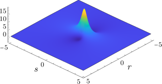
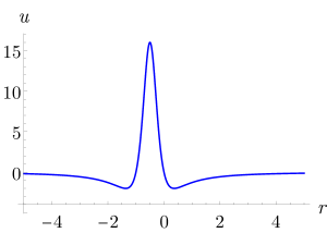
Figure 1: $1$-lump solution of the KPI equation:  $a=\gamma_{1}=0,b=1$. Right: Vertical cross-section showing the maximum and two minima.

Notice that the solution is stationary in the $rs$-plane since the only time dependence enters via the co-moving coordinates $x^{\prime},y^{\prime}$. Hence, (2.17) represents a rational traveling waveform with a single peak (maximum) at $(r_{0}-{\textstyle\frac{1}{2b}},s_{0})$, of height $16b^{2}$, and two local minima symmetrically located from the peak at $(r_{0}-{\textstyle\frac{1}{2b}}\pm{\textstyle\frac{\sqrt{3}}{2b}},\,s_{0})$ and depth $-2b^{2}$ determined by $b$ and the complex parameter $\gamma_{1}$ as illustrated in Figure 1. The wave moves in the $xy$-plane with a uniform velocity $(3(a^{2}+b^{2}),-3a)$ at an angle $\tan^{-1}(-a/(a^{2}+b^{2}))$ with the positive $x$-axis. This solution is referred to as the $1$-lump solution since it has a single peak which also coincides with the fact that $N=1$ in this case. It will be shown in Section 4 that $N$ indeed represents the number of peaks when $|t|\gg 1$ for this class of rational solutions.

Since $u_{1}$ is the $x$-derivative of the rational function $F_{1x}/F_{1}$ which decays as $|x|\to\infty$ for all $y,t$, one has that $\int_{-\infty}^{\infty}u_{1}\,dx=0$. However, $u_{1}$ is not a $L^{1}(\mathbb{R}^{2})$ function although $u_{1}\in L^{2}(\mathbb{R}^{2})$ and $\int\!\!\int_{\mathbb{R}^{2}}u_{1}^{2}=16\pi b$; the latter is a conserved quantity for the KPI equation (1.1).

2.3.2 A 2-lump solution

Next we consider the simplest case for $n=2$ where $m_{1}=1,m_{2}=2$. Here $M$ is a $2\times 2$ matrix and there are 2 column vectors in $P$ which is a $3\times 2$ matrix. The matrices $P,U$ and $D$ are given by

$$P=\begin{pmatrix}p_{1}&p_{2}\\ ip_{0}&ip_{1}\\ 0&-p_{0}\end{pmatrix}\,,\quad\qquad U=\begin{pmatrix}1&{\textstyle\frac{1}{2b}}&{\textstyle\frac{1}{4b^{2}}}\\ 0&1&{\textstyle\frac{1}{b}}\\ 0&0&1\end{pmatrix}\,,\qquad\quad D=\mathrm{diag}(1,\,\,{\textstyle\frac{1}{2b}},\,\,{\textstyle\frac{1}{4b^{2}}})$$

from which the $2\times 2$ minors are computed as follows:

$$P({\bf 0})=P(01)=i(p_{1}^{2}-p_{0}p_{2}),\,\,P(02)=-p_{1}p_{0},\,\,P(12)=-ip_{0}^{2},$$

$$U\tbinom{01}{01}=U\tbinom{02}{02}=U\tbinom{12}{12}=1,\quad U\tbinom{02}{01}=U\tbinom{12}{01}=U\tbinom{12}{02}=0,\quad U\tbinom{01}{02}={\textstyle\frac{1}{b}}=2U\tbinom{02}{12},\quad U\tbinom{01}{12}={\textstyle\frac{1}{4b^{2}}}\,.$$

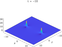
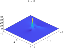
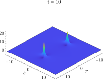
Figure 2: A $2$-lump solution interacting in the $rs$-plane corresponding to $\tau_{2}$ in (2.18). Parameters:  $a=\gamma_{1}=\gamma_{2}=0,b=1$.

From (2.4) it follows that $P(01),P(02)$ and $P(12)$ are weighted homogeneous polynomials in $\theta_{1},\theta_{2}$ of degree $(m_{1}+m_{2})-|{\bf r}|$, with $|{\bf r}|=r_{1}+r_{2}=1,2,3$, respectively, as shown in Section 2.2. Next, calculating the minors using (2.13b) leads to the sum of squares expression for the $\tau$-function

$$\tau_{P}=\frac{|Q(01)|^{2}}{(2b)^{2}}+\frac{|Q(02)|^{2}}{(2b)^{4}}+\frac{|Q(12)|^{2}}{(2b)^{6}}={\textstyle\frac{1}{4b^{2}}}\left[|({\textstyle\frac{\theta_{1}^{2}}{2}}-\theta_{2})+{\textstyle\frac{1}{b}}\theta_{1}-{\textstyle\frac{1}{4b^{2}}}|^{2}+{\textstyle\frac{1}{4b^{2}}}|\theta_{1}+{\textstyle\frac{i}{2b}}|^{2}+{\textstyle\frac{1}{16b^{4}}}\right]\,,$$

where (2.4) is used to express $p_{0}=1,p_{1},p_{2}$. Note that $\tau_{P}$ is a weighted homogeneous polynomial of degree $2(m_{1}+m_{2})=6$ in $\theta_{1},\theta_{2},b$ as mentioned below (2.13a). Finally using (2.16) and factoring out ${\textstyle\frac{1}{4b^{2}}}$ from $\tau_{P}$ above one obtains the reduced $\tau$-function

$$\tau_{2}=|{\textstyle\frac{1}{2}}((r+{\textstyle\frac{1}{b}})^{2}-s^{2})-3bt-{\textstyle\frac{1}{4b^{2}}}+i(r+{\textstyle\frac{3}{2b}})s|^{2}+{\textstyle\frac{1}{4b^{2}}}|(r+{\textstyle\frac{1}{2b}})+is|^{2}+{\textstyle\frac{1}{16b^{4}}}\,,$$ (2.18)

where we have set the constants $\gamma_{1}=\gamma_{2}=0$ for simplicity. In terms of the variables $r,s,t$ (equivalently, $x,y,t$) and $b=\mathop{\rm Im}\nolimits(k)$, $\tau_{2}$ is a weighted homogeneous polynomial of degree $2N$ with $N=(m_{1}+m_{2})-{\textstyle\frac{n(n-1)}{2}}=2$ as in Proposition 2.1. The leading order (in $r,s,t$) contribution arises from the from the first square term $|Q({\bf 0})|^{2}$ through $P({\bf 0})=i\big{(}{\textstyle\frac{1}{2}}\theta_{1}^{2}-\theta_{2}\big{)}$ which is of degree $N=2$ in $\theta_{1},\theta_{2}$.

Notice that unlike $\tau_{1}$, the polynomial $\tau_{2}(r,s,t)$ in (2.18) does depend explicitly on $t$ so that the solution $u_{2}$ obtained from (2.6) is non-stationary in the co-moving $rs$-plane. The explicit expression for $u_{2}(x,y,t)$ is complicated, so it is not included here. Figure 2 illustrates that $u_{2}$ consists of 2 localized lumps (local maxima) along the $s$-axis that are well separated as $t\ll-1$; these lumps get attracted to each other and overlap for finite $t$ to form a transient large amplitude peak that splits again into two localized lumps which then recede from each other when $t\gg 1$ but along the $r$-axis. Furthermore, the height of each peak also evolve with time and approaches the constant height of the 1-lump solution as $|t|\to\infty$. The interaction process is an example of anomalous scattering rather than the usual solitonic interaction of the simple $n$-lump solutions of KPI found in [30]. This particular $2$-lump solution and another solution which corresponds to $n=1,m_{1}=2$, were found earlier in [20, 45, 3]. The latter solution was also studied more recently in [10], where the structure of the solution was analyzed in details. The analysis for the solutions corresponding to $\tau_{2}$ in (2.18) is similar, so we do not include it here. The locations of the lump peaks for these two solutions are related by time reversal symmetry $t\to-t$ when $|t|\gg 1$. Note that $N=2$ in both cases. The classification scheme developed in Section 3 will establish that there are only 2 possible $2$-lump solutions obtained from the method outlined in Section 2.2.

2.3.3 A $3$-lump solution

Our next illustrative example is $n=2,m_{1}=1,m_{2}=3$ which corresponds to $N=3$. In this case, the matrices $P,U,D$ are as follows:

$$P=\begin{pmatrix}p_{1}&p_{3}\\ ip_{0}&ip_{2}\\ 0&-p_{1}\\ 0&-ip_{0}\end{pmatrix}\,,\quad\qquad U=\begin{pmatrix}1&{\textstyle\frac{1}{2b}}&{\textstyle\frac{1}{(2b)^{2}}}&{\textstyle\frac{1}{(2b)^{3}}}\\ 0&1&{\textstyle\frac{2}{2b}}&{\textstyle\frac{3}{(2b)^{2}}}\\ 0&0&1&{\textstyle\frac{3}{2b}}\\ 0&0&0&1\end{pmatrix}\,,\qquad\quad D=\mathrm{diag}\big{(}1,\,\,{\textstyle\frac{1}{(2b)^{2}}},\,\,{\textstyle\frac{1}{(2b)^{4}}}\,\,{\textstyle\frac{1}{(2b)^{6}}}\big{)}\,,$$

and the index set for the maximal minors ${\bf r}=(r_{1}r_{2})\in\{(01),(02),(03),(12),(13),(23)\}$. Then using (2.13b) and (2.4) the $\tau$-function can be expressed as

$$\tau_{3}=(2b)^{2}\tau_{P}=|({\textstyle\frac{\theta_{1}^{3}}{3}}-\theta_{3})+{\textstyle\frac{i}{b}}(\theta_{1}+{\textstyle\frac{i}{2b}})^{2}|^{2}+{\textstyle\frac{1}{(2b)^{2}}}|(\theta_{1}+{\textstyle\frac{i}{b}})^{2}+{\textstyle\frac{1}{4b^{2}}}|^{2}+{\textstyle\frac{1}{(2b)^{4}}}|2(\theta_{1}+{\textstyle\frac{i}{b}})|^{2}+{\textstyle\frac{1}{(2b)^{6}}}\,.$$ (2.19)

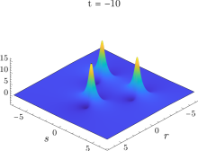
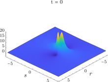
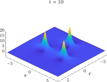
Figure 3: $3$-lump solution of the KPI equation:  $a=\gamma_{1}=\gamma_{2}=\gamma_{3}=0,b=1$.

Figure 3 shows that the corresponding KPI solution $u_{3}(x,y,t)$ is a $3$-lump solution which forms a triangular pattern in the $rs$-plane for $|t|\gg 1$ with the 3 peaks located at the vertices of the triangle. As time progresses starting from large negative values, the lumps are attracted to each other and overlap, then for $t\gg 1$ the 3 peaks re-appear and recede from each other forming a time-reversed triangular structure. One of the peaks is located along the $r$-axis while the other two are located symmetrically from the $r$-axis. It will be shown in Section 4 that the approximate peak locations for $|t|\gg 1$ can be estimated from the zeros of the first $|\cdot|^{2}$ term i.e., by setting $Q({\bf 0})=0$ in (2.19). Indeed, after substituting (2.16) in (2.19), $Q({\bf 0})=0$ implies that $(z+{\textstyle\frac{1}{b}})^{3}+3t-{\textstyle\frac{1}{4b^{3}}}=0$ where $z=r+is$. The peak locations are then given by

$$z_{j}=r_{j}+is_{j}\sim-\frac{1}{b}+x_{j}t^{1/3}+\frac{1}{12x_{j}^{2}b^{3}}t^{-2/3}+O(|t|^{-5/3})\,,\quad\qquad|t|\gg 0\,,$$

where $x_{j},\,j=1,2,3$ are the roots of $x^{3}+3=0$. These are shown in Figure 4. Note from Figure 4 that the peak locations exhibit reflection symmetry across the line $r=-{\textstyle\frac{1}{b}}$ as $t\to-t$.

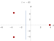
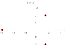
Figure 4: $3$-lump peak locations at $t=-40$ (left panel) and $t=40$ (right panel). Black dots represent locations $z_{j}$ where $Q({\bf 0})=0$, red open circles are exact locations. As $t\to-t$, the peak locations are reflected across the vertical line $r=-{\textstyle\frac{1}{b}}$. KP parameters: same as in Figure 3.

Finally, we remark that in local co-ordinates $(r,s)=(r_{j}+h,s_{j}+k),\,\,(h,k)\sim O(1)$ near each peak, $\tau_{3}$ in (2.19) reduces to a $1$-lump $\tau$-function $\tau_{1}(h,k)$ for $|t|\gg 1$. Specifically, $\tau_{3}\sim(3|t|)^{4/3}\left(h^{2}+k^{2}+{\textstyle\frac{1}{4b^{2}}}+O(|t|^{-1/3})\right)$. This implies that the $3$-lump solution $u_{3}$ is a superposition of three $1$-lump solution as $|t|\to\infty$. This result also holds for general multi-lumps as will be shown in Section 4.2.

3 Classification of KPI multi-lumps

In this section we provide a simple yet useful characterization of the KPI rational solutions constructed in Section 2.2, in terms of integer partitions. Then we classify these solutions utilizing certain ideas from the integer partition theory. Given a set of distinct positive integers $\{m_{1},\ldots,m_{n}\}$ indexing the generalized Schur polynomials $p_{m_{i}},\,i=1,\ldots,n$, the key observation is that there is a one-to-one correspondence between the $\tau$-function $\tau_{P}$ and the leading order principal minor $P({\bf 0})$. Indeed, from $P({\bf 0})=i^{|{\bf 0}|}W({\bf 0})$ where the determinant $W({\bf 0})$ is given by (2.14), one can immediately identify the generalized Schur polynomials $p_{m_{i}}$ which are used to construct the KPI solution as in (2.9). On the other hand, $P({\bf 0})$ can be extracted from the first square term of the expression of $\tau_{P}$ in (2.13b), or even directly from (2.11) as the leading principal minor of the matrix $P$ which is used to construct the Gram matrix $H$ in (2.10) that then yields the $\tau$-function $\tau_{P}=\det H$ in (2.13b).

3.1 Characterization of multi-lumps via integer partition

In order to establish the relationship between the KPI lumps and partitions of integers we first introduce some basic ideas from partition theory and its connection with the symmetric polynomials.

Definition 3.1 (Partition).

A partition is a decomposition of a nonnegative integer $N$ given by a non-decreasing sequence $\lambda=(\lambda_{1},\ldots\lambda_{n})$ such that $0\leq\lambda_{1}\leq\lambda_{2}\leq\cdots\leq\lambda_{n}$ and $|\lambda|:=\lambda_{1}+\cdots+\lambda_{n}=N$. The number of non-zero parts $l(\lambda)\leq n$ of $\lambda$ is called its length and $|\lambda|=N$, its size. The strictly increasing sequence $m=(m_{1},\ldots,m_{n})$ defined by $m_{j}=\lambda_{j}+(j-1),\,\,j=1,\ldots,n$ is called the degree vector of the partition $\lambda$.

It is often convenient to describe a partition $\lambda$ of $N\in\mathbb{N}$ in terms of its associated Young diagram $Y_{\lambda}$ which is a rectangular array of left-justified boxes (or dots) such that the i^th row from the top contains $\lambda_{n-i+1}$ boxes, $i=1,\ldots,n$. Thus $Y_{\lambda}$ consists of $n$ rows, $l(\lambda)$ of which contain non-zero number of boxes, and $\lambda_{n}$ columns. The total number of boxes in $Y_{\lambda}$ is, of course $N$. The conjugate $\lambda^{\prime}$ of a partition $\lambda$ is a partition whose Young diagram $Y_{\lambda^{\prime}}$ is the transpose of $Y_{\lambda}$ obtained by interchanging its rows and columns. Clearly, $|\lambda^{\prime}|=|\lambda|=N,(\lambda^{\prime})^{\prime}=\lambda$, the length $l(\lambda^{\prime})=\lambda_{n}$, also $\lambda^{\prime}$ has $l(\lambda)\leq n$ columns. A partition is called self-conjugate if $\lambda=\lambda^{\prime}$.

Example 3.1.

Following are the Young diagrams of the partition $\lambda=(1,2,4)$, its conjugate $\lambda^{\prime}=(1,1,2,3)$ and a self-conjugate partition $\mu=(1,2,3)$ also known as a staircase (or triangular) partition.

$$Y_{\lambda}=\raisebox{5.0pt}{\ytableausetup{boxsize=0.8em}\ydiagram{4,2,1}}\hskip 72.26999ptY_{\lambda^{\prime}}=\raisebox{8.50006pt}{\ytableausetup{boxsize=0.8em}\ydiagram{3,2,1,1}}\hskip 72.26999ptY_{\mu}=\raisebox{5.0pt}{\ytableausetup{boxsize=0.8em}\ydiagram{3,2,1}}$$

Here, $|\lambda|=|\lambda^{\prime}|=7$ which is the number of boxes in the diagrams $Y_{\lambda}$ and $Y_{\lambda^{\prime}}$. The number of non-zero rows in $Y_{\lambda}=l(\lambda)=3=$ number of columns in $Y_{\lambda^{\prime}}$. Similarly, the number of non-zero rows in $Y_{\lambda^{\prime}}=l(\lambda^{\prime})=4=\lambda_{4}=$ number of columns in $Y_{\lambda}$. For the self-conjugate partition, $|\mu|=6$, and $l(\mu)=3=\mu_{3}$.

For a given pair of partitions $\mu$ and $\lambda$, $\mu\subset\lambda$ means that $Y_{\mu}\subset Y_{\lambda}$, i.e., $\mu^{i}\leq\lambda^{i},\,\,1\leq i\leq l(\mu)$ where $\mu^{i},\lambda^{i}$ are the number of boxes in the i^th row (from top) of $Y_{\mu},Y_{\lambda}$, respectively. Alternatively, suppose $\lambda$ has $n$ parts then the number of parts in $\mu$ can be extended to $n$ by appending $0$ parts if necessary. Then $\mu\subset\lambda$ implies $\mu_{i}\leq\lambda_{i},\,\,1\leq i\leq n$. The set difference $Y_{\lambda}-Y_{\mu}$ is called a skew diagram $Y_{\lambda/\mu}$ which may be disconnected.

Example 3.2.

Let $\lambda=(1,3,4)$ and $\mu=(1,2)$ then

$$Y_{\lambda}=\raisebox{5.0pt}{\ytableausetup{boxsize=0.8em}\ydiagram{4,3,1}}\hskip 72.26999ptY_{\mu}=\raisebox{3.00003pt}{\ytableausetup{boxsize=0.8em}\ydiagram{2,1}}\hskip 72.26999ptY_{\lambda/\mu}=\raisebox{5.0pt}{\ytableausetup{boxsize=0.8em}\ydiagram{2+2,1+2,1}}$$

If $\rho=(2,3)$ but $\lambda$ is the same as above then

$$Y_{\rho}=\raisebox{3.00003pt}{\ytableausetup{boxsize=0.8em}\ydiagram{3,2}}\hskip 72.26999ptY_{\lambda/\rho}=\raisebox{5.0pt}{\ytableausetup{boxsize=0.8em}\ydiagram{3+1,2+1,1}}$$

Schur and skew-Schur functions:  Associated with each partition $\lambda$ of $N\in\mathbb{N}$ and degree vector $m=(m_{1},\ldots,m_{n})$, there is a unique weighted homogeneous polynomial of degree $N$ in the variables $\theta_{j}$ defined by the second $n\times n$ determinant in (2.14) namely, $W({\bf 0})=\det(p_{m_{j}-i+1})=\det(p_{\lambda_{j}+j-i})$. It will be referred to as the Schur function throughout this article and will be denoted by $W_{\lambda}$. Historically, the Schur functions were introduced in the study of symmetric functions in $n$ variables $(x_{1},\ldots,x_{n})$ with integer coefficients, and was defined as a quotient of determinants namely $W_{\lambda}(x_{1},\ldots,x_{n})=\det(x_{i}^{m_{j}})/\det(x_{i}^{j-1})$. The last formula can be re-expressed via Jacobi-Trudi identity as $W_{\lambda}=\det(h_{\lambda_{j}+j-i})$ where $h_{r}=\sum x_{i_{1}}\cdots x_{i_{r}}$, $1\leq i_{1}\leq\cdots\leq i_{r}\leq n$ are the complete symmetric polynomials of degree $r$. Next, introducing the power sums $\theta_{j}={\textstyle\frac{1}{j}}(x_{1}^{j}+\cdots+x_{n}^{j}),\,j\geq 1$ it can be shown that $h_{r}(x_{1},\ldots,x_{n})=p_{r}(\theta_{1},\ldots,\theta_{r})$, and one recovers the expression for $W_{\lambda}$ in terms of the generalized Schur polynomials $p_{r}$.

Just as each Young diagram $Y_{\lambda}$ is associated to the Schur function $W_{\lambda}$, similarly each skew diagram $Y_{\lambda/\mu}$ is associated with a skew Schur function defined as follows. Let $\lambda,\mu$ be two partitions with degree vectors $m$ and $n$, i.e., $m_{i}=\lambda_{i}+(i-1),\,n_{i}=\mu_{i}+(i-1),\,\,i=1,\ldots,n$, and let $\mu\subset\lambda$. Then the Schur function $W_{\lambda}$ and the skew Schur function $W_{\lambda/\mu}$ are defined as

$$W_{\lambda}=\det(p_{m_{j}-i+1})=\mathop{\rm Wr}\nolimits(p_{m_{1}},\ldots,p_{m_{n}})\,,\qquad W_{\lambda/\mu}=\det(p_{m_{j}-n_{i}})=\det(p_{\lambda_{j}-\mu_{i}+j-i})\,,$$ (3.1)

where the wronskian in the first expression is with respect to $\theta_{1}$, and is the same epression as $W({\bf 0})$ in (2.14). Both $W_{\lambda}$ and $W_{\lambda/\mu}$ are weighted homogeneous polynomials in the $\theta_{j}$s of degree $|\lambda|$ and $|\lambda|-|\mu|$ respectively, which are also equal to the number of boxes in the Young diagram $Y_{\lambda}$ and the skew diagram $Y_{\lambda/\mu}$. It follows that if $\mu=\lambda$ i.e., $Y_{\lambda}-Y_{\mu}=\emptyset$ (a diagram with no boxes) then $W_{\emptyset}=\mathop{\rm Wr}\nolimits(p_{0},p_{1},\ldots,p_{n-1})=1$. Also, if $\mu=\emptyset$ then $W_{\lambda/\emptyset}=W_{\lambda}$, and if $\mu\supset\lambda$ then $W_{\lambda/\mu}=0$. The Schur functions $W_{\lambda}$ forms a basis of the symmetric functions over the ring of integers. The Schur function together with its properties and its role in the representation theory of the symmetric group $S_{N}$ are well documented in the literature [33, 18, 29] (and references therein).

Notice that the multi-index sets ${\bf r}=(r_{1}\ldots r_{n})$ with $0\leq r_{1}<r_{2}<\cdots<r_{n}\leq m_{n}$ introduced to label the $n\times n$ minors in (2.13b) form the degree vector of a partition denoted by $\lambda({\bf r})$. Each part $\lambda_{i}({\bf r})=r_{i}-i+1$ for $1\leq i\leq n$ and $|\lambda({\bf r})|=|{\bf r}|-|{\bf 0}|$ where recall that $|{\bf r}|=r_{1}+\cdots+r_{n}$. Furthermore, in addition to the lexicographic ordering in Definition 2.1, there is a natural partial ordering among the multi-index sets defined by

$${\bf r}\preceq{\bf s}\quad\Leftrightarrow\quad r_{i}\leq s_{i}\,,\qquad 1\leq i\leq n\,.$$

The corresponding partitions then satisfy $\lambda({\bf r})\subset\lambda({\bf s})$ and are partially ordered by the inclusion $Y_{\lambda({\bf r})}\subset Y_{\lambda({\bf s})}$ of the corresponding Young diagrams as mentioned after Example 3.1. Note that if ${\bf r}={\bf 0}$ then the partition $\lambda({\bf 0})=\emptyset$ which has only $0$ parts, and when ${\bf r}={\bf m}$ the last multi-index in the lexicographic order, $\lambda({\bf m})=\lambda$.

Example 3.3.

Consider the multi-index sets of Example 2.1. The ordering described above corresponds to the partially ordered set (poset) shown below where the arrows indicate the ordering ${\bf r}\preceq{\bf s}$.

$$\begin{matrix}&&\quad\nearrow&\raisebox{7.22743pt}{(03)}&\searrow&\\ (01)&\rightarrow&(02)&&(13)&\rightarrow&(23)\,,\\ &&\quad\searrow&\raisebox{-7.22743pt}{(12)}&\nearrow&\\ \end{matrix}$$

Note that the index sets $(03)$ and $(12)$ are incomparable although both $(03)\preceq(13),\,\,(12)\preceq(13)$. The partitions $\lambda({\bf r})$ corresponding to ${\bf r}=(r_{1}r_{2})$ are given by
$\lambda((01))=(0,0)=\emptyset,\quad\lambda((02))=(0,1),\quad\lambda((03))=(0,2),\quad\lambda((12))=(1,1),\quad\lambda((13))=(1,2)$, and $\lambda((23))=(2,2)$. Then the associated Young diagrams are

$$Y_{\emptyset}\,,\qquad Y_{(0,1)}=\ytableausetup{boxsize=0.6em}\ydiagram{1}\,,\qquad Y_{(0,2)}=\ytableausetup{boxsize=0.6em}\ydiagram{2}\,,\qquad Y_{(1,1)}=\raisebox{3.99994pt}{\ytableausetup{boxsize=0.6em}\ydiagram{1,1}}\,,\qquad Y_{(1,2)}=\raisebox{3.99994pt}{\ytableausetup{boxsize=0.6em}\ydiagram{2,1}}\,,\qquad Y_{(2,2)}=\raisebox{3.99994pt}{\ytableausetup{boxsize=0.6em}\ydiagram{2,2}}\,.$$

Notice that neither $Y_{(0,2)}$ nor $Y_{(1,1)}$ are contained in each other but both are subdiagrams of $Y_{(1,2)}$.

The main purpose of the background in partition theory is to relate the expressions for the KPI $\tau$-function $\tau_{P}$ in (2.13b) with the Schur and skew Schur functions. It was already mentioned earlier that in (3.1) $W_{\lambda}=W({\bf 0})$ which is the second determinant in (2.14). The second formula in (3.1) states that for a given multi-index set ${\bf r}$ and the associated partition $\mu=\lambda({\bf r})$ the skew Schur function $W_{\lambda/\mu}=W_{\lambda/\lambda({\bf r})}=W({\bf r})$ where $W({\bf r})$ is the first determinant in (2.13b). Then using the fact that the $n\times n$ minors of the upper triangular matrix $U$ in (2.13a) satisfy $U\tbinom{{\bf r}}{{\bf s}}=0$ unless ${\bf r}\preceq{\bf s}$, the minors in (2.13b) can now be re-expressed in terms of the Schur and the skew Schur functions in the following manner

$$Q({\bf 0})=i^{|{\bf 0}|}\Big{(}W_{\lambda}+\sum_{\lambda(s)\neq\emptyset}\!\!i^{|\lambda(s)|}U\tbinom{{\bf 0}}{{\bf s}}W_{\lambda/\lambda({\bf s})}\Big{)}\,,$$ (3.2a)

where the sum is over all non-empty partitions $$\lambda({\bf s}) \lambda({\bf s})\subset\lambda Y_{\lambda} W_{\lambda/\lambda({\bf s})} \theta_{j} |\lambda|-|\lambda({\bf s})|,\,\,1\leq|\lambda({\bf s})|\leq|\lambda| W_{\lambda/\lambda({\bf s})}=0 \lambda({\bf s})\supset\lambda {\bf r}>{\bf 0}$$. If , i.e., partitions whose Young diagram is contained in , then the corresponding skew Schur function is a weighted homogeneous polynomial in the of degree . Otherwise, when . Similarly, for each , the second expression in (2.13b) gives

$$Q({\bf r})=i^{|{\bf r}|}\Big{(}W_{\lambda/\lambda({\bf r})}+\sum_{\lambda({\bf s})}i^{|\lambda({\bf s})|-|\lambda({\bf r})|}U\tbinom{{\bf r}}{{\bf s}}W_{\lambda/\lambda({\bf s})}\Big{)}\,,\qquad\lambda({\bf r})\subset\lambda({\bf s})\subseteq\lambda\,,$$ (3.2b)

where the sum is over all $$\lambda({\bf s}) Y_{\lambda({\bf r})}\subset Y_{\lambda({\bf s})}\subseteq Y_{\lambda} W_{\lambda/\lambda({\bf s})} \theta_{j} |\lambda|-|\lambda({\bf s})| |\lambda({\bf r})|<|\lambda({\bf s})|\leq|\lambda|$$ such that the Young diagrams satisfy . The skew Schur functions in this sum are weighted homogeneous polynomials in the of degree with .

Example 3.4.

Consider the $3$-lump solution in Section 2.3.3. In this case, the partition corresponding to the degree vector $m=(m_{1},m_{2})=(1,3)$ is $\lambda=(1,2)$. The $2\times 2$ minors of $P,Q,U$ and $D$ are labeled by the set of multi-indices $\{{\bf r}=(r_{1}r_{2})\}$ which corresponds to the poset in Example 3.3. Using the partitions $\lambda({\bf r})$ enumerated in Example 3.3 and employing either equation (2.14) or (3.1), the Schur function $W_{(1,2)}=W({\bf 0})$ and the skew schur functions $W_{\lambda/\lambda({\bf r})}=W({\bf r})$ for this example are found to be

$$W((01))=W_{(1,2)}=\begin{vmatrix}p_{1}&p_{3}\\ p_{0}&p_{2}\end{vmatrix}\,,\quad W((02))=W_{(1,2)/(0,1)}=\begin{vmatrix}p_{1}&p_{3}\\ 0&p_{1}\end{vmatrix}\,,\quad W((03))=W_{(1,2)/(0,2)}=\begin{vmatrix}p_{1}&p_{3}\\ 0&p_{0}\end{vmatrix}\,,$$

$$W((12))=W_{(1,2)/(1,1)}=\begin{vmatrix}p_{0}&p_{2}\\ 0&p_{1}\end{vmatrix}\,,\quad W((13))=W_{(1,2)/(1,2)}=\begin{vmatrix}p_{0}&p_{2}\\ 0&p_{0}\end{vmatrix}\quad W((23))=W_{(1,2)/(2,2)}=\begin{vmatrix}0&p_{1}\\ 0&p_{0}\end{vmatrix}\,,$$

Notice that $W_{(1,2)/(1,2)}=W_{\emptyset}=1$ and $W_{(1,2)/(2,2)}=0$ since the partition $(2,2)\supset(1,2)$. Then from (3.2a) and the matrix $U$ given in Section 2.3.3,

$$Q({\bf 0})=Q((01))=i\big{[}W_{(1,2)}+{\textstyle\frac{i}{b}}W_{(1,2)/(0,1)}-{\textstyle\frac{3}{4b^{2}}}W_{(1,2)/(0,2)}-{\textstyle\frac{1}{4b^{2}}}W_{(1,2)/(1,1)}-{\textstyle\frac{i}{4b^{3}}}W_{\emptyset}\big{]}\,,$$

which is the argument inside the leading $|\cdot|^{2}$ term of $\tau_{3}$ in (2.19) when expressed in terms of $\theta_{j}$. The arguments inside the remaining $|\cdot|^{2}$ terms in $\tau_{3}$ are obtained from (3.2b). For example,

$$Q((02))=-\big{[}W_{(1,2)/(0,1)}+{\textstyle\frac{3i}{2b}}W_{(1,2)/(0,2)}+{\textstyle\frac{i}{2b}}W_{(1,2)/(1,1)}-{\textstyle\frac{3}{4b^{2}}}W_{\emptyset}\big{]}\,,$$

and the rest follow in a similar fashion.

We rename the KPI $\tau$-function $\tau_{P}$ as $\tau_{\lambda}$. Then the characterization of $\tau_{\lambda}$ in terms of integer partition can be stated as follows.

Proposition 3.1.

Let $\lambda=(\lambda_{1},\ldots,\lambda_{n})$ be a partition of a positive integer $N$ and $W_{\lambda}$ be the associated Schur function. Then there is a unique (upto a $GL(n,\mathbb{C})$ gauge freedom) KPI $\tau$-function given by (2.13b) and (3.2b)

$$\tau_{\lambda}=\frac{1}{(2b)^{2|{\bf 0}|}}\Big{|}W_{\lambda}+\sum_{\lambda(s)\neq\emptyset}\!\!i^{|\lambda(s)|}U\tbinom{{\bf 0}}{{\bf s}}W_{\lambda/\lambda({\bf s})}\Big{|}^{2}+\sum_{{\bf r}>{\bf 0}}\frac{1}{(2b)^{2|{\bf r}|}}\Big{|}W_{\lambda/\lambda({\bf r})}+\sum_{\lambda({\bf r})\subset\lambda({\bf s})\subseteq\lambda}\!\!\!i^{|\lambda({\bf s})|-|\lambda({\bf r})|}U\tbinom{{\bf r}}{{\bf s}}W_{\lambda/\lambda({\bf s})}\Big{|}^{2}\,,$$

where ${\bf r}=(r_{1}\ldots r_{n}),\,\,0\leq r_{1}<\cdots<r_{n}\leq m_{n}$ is the degree vector of the partition $\lambda({\bf r})$. $\tau_{\lambda}$ is expressed as a sum of squares, where each square term is a weighted homogeneous polynomial in $\theta_{j},\,j=1,\ldots,\lambda_{n}+n-1$ and their complex conjugates, of degree $2(|\lambda|-|\lambda({\bf r})|),\,\,0\leq|\lambda({\bf r})|\leq|\lambda|$ with $|\lambda|=N$.

Remark 3.1.

• Throughout this article the parts $\lambda_{j}$ of a partition $\lambda=(\lambda_{1},\ldots,\lambda_{n})$ are consistently listed in non-decreasing order (cf. Definition 3.1) contrary to the more standard convention of listing the parts in non-increasing order.

• Yet another way to denote a partition of a positive integer $N$ is to indicate the number of times (multiplicity) each positive integer $1,2,\ldots$ occur as a part in the partition. That is, $\lambda=(1^{\alpha_{1}},2^{\alpha_{2}},\ldots,N^{\alpha_{N}})$, where $\alpha_{i}\geq 0,\,\,i=1,2,\ldots,N$ satisfy $\alpha_{1}+2\alpha_{2}+\cdots N\alpha_{N}=N=|\lambda|$. Let $Y_{\lambda}$ be the Young diagram of $\lambda$. The sum of boxes in each column of $Y_{\lambda}$ starting from the leftmost column is successively given by $\mu_{N}=\alpha_{1}+\cdots+\alpha_{N},\,\,\mu_{N-1}=\alpha_{2}+\cdots+\alpha_{N},\ldots\,\,\mu_{1}=\alpha_{N}$ so that $\mu_{1}\leq\mu_{2}\leq\cdots\mu_{N}$. Thus, $\mu=(\mu_{1},\ldots,\mu_{N})$ is also a partition with $|\mu|=N$. In fact, $\mu=\lambda^{\prime}$ is the partition conjugate to $\lambda$ where the difference between successive rows from the top $\mu_{j}-\mu_{j-1}=\alpha_{N-j+1},\,\,j=N,N-1,\ldots,2,\,\mu_{1}=\alpha_{N}$.

• The Schur function $W_{\lambda}$ is a wronskian as shown in (3.1) but the skew Schur functions $W_{\lambda/\mu}$ are not wronskians. They are in fact, components of the $n$-form $\omega_{P}$ representing the Grassmannian $P\in{\rm Gr}_{\mathbb{C}}(n,m_{n}+1)$ introduced in Section 2.2. However, viewed as functions of $\theta=(\theta_{1},\theta_{2},\ldots)$, it can be shown that $W_{\lambda/\mu}(\theta)=W_{\mu}(\tilde{\partial})W_{\lambda}(\theta)$, where $\tilde{\partial}=(\partial_{\theta_{1}},{\textstyle\frac{1}{2}}\partial_{\theta_{2}},{\textstyle\frac{1}{3}}\partial_{\theta_{3}},\ldots)$ [27].

3.2 The $N$-lump solutions

Propositions 2.1 and 3.1 demonstrate that the $\tau$-function $\tau_{\lambda}$ and the corresponding rational solution of KPI given by (2.6) can be identified with a partition $\lambda$ of a positive integer $N$. In particular, each $\tau_{\lambda}$ is uniquely characterized by its Schur function $W_{\lambda}$ which is a weighted homogeneous polynomial in $\theta_{j}$ of degree $|\lambda|=N$. Henceforth in this paper, we refer to these solutions as the $N$-lump solutions. Our nomenclature will be further justified in Section 4 where it will be shown that the $N$-lump solution separates into $N$ distinct peaks whose heights approach the $1$-lump peak height asymptotically as $|t|\to\infty$. Evidence of the latter feature has already been seen in the examples of Section 2.3. The $N$-lump solutions for a given positive integer $N$ can be enumerated according to the underlying partition $\lambda$ of $N$. To avoid redundancies, we will consider only those partitions $\lambda=(\lambda_{1},\ldots,\lambda_{n})$ in this subsection, whose smallest part $\lambda_{1}>0$ so that the length of the partition $l(\lambda)=n$. It will be useful to introduce a lexicographic ordering among the partitions of the same size $|\lambda|=N$ in a similar way as in Definition 2.1.

Definition 3.2.

(Lexicographic ordering) Let $\lambda$ and $\mu$ be two distinct partitions of $N$. If $j$ is the earliest index such that $\mu_{j}\neq\lambda_{j}$ then $\mu<\lambda$ if and only if $\mu_{j}<\lambda_{j}$.

Note that the lexicographic ordering is a total ordering. The smallest partition $\lambda=(1,1,\ldots,1):=(1^{N})$ which has $N$ parts, and the largest partition $\lambda=(N)$ that has only one part.

Example 3.5.

All possible partitions for $N=4$ are:  $(1^{4})<(1^{2},2)<(1,3)<(2^{2})<(4)$ and the associated Young diagrams are given by

$$Y_{(1^{4})}=\raisebox{10.00002pt}{\ytableausetup{boxsize=0.6em}\ydiagram{1,1,1,1}}\,,\qquad Y_{(1^{2},2)}=\raisebox{6.00006pt}{\ytableausetup{boxsize=0.6em}\ydiagram{2,1,1}}\,,\qquad Y_{(1,3)}=\raisebox{3.99994pt}{\ytableausetup{boxsize=0.6em}\ydiagram{3,1}}\,,\qquad Y_{(2^{2})}=\raisebox{3.99994pt}{\ytableausetup{boxsize=0.6em}\ydiagram{2,2}}\,,\qquad Y_{(4)}=\ytableausetup{boxsize=0.6em}\ydiagram{4}\,.$$

There are two conjugate pairs, namely $(1^{4})^{\prime}=(4),\,(1^{2},2)^{\prime}=(1,3)$, while $(2^{2})$ is self-conjugate. Hence there are 5 types of $4$-lump solutions indexed by the Schur functions:  $W_{(1^{4})}=\mathop{\rm Wr}\nolimits(p_{1},p_{2},p_{3},p_{4}),\,\,W_{(1^{2},2)}=\mathop{\rm Wr}\nolimits(p_{1},p_{2},p_{4}),\,\,W_{(1,3)}=\mathop{\rm Wr}\nolimits(p_{1},p_{4}),\,\,W_{(2^{2})}=\mathop{\rm Wr}\nolimits(p_{2},p_{3}),\,\,W_{(4)}=p_{4}$. In each case, $W_{\lambda}$ is a weighted homogeneous polynomial in $\theta_{j},\,\,j=1,\ldots,4$ of degree 4.

For a given positive integer $N$, the total number of distinct $N$-lump solutions of the KPI equation is given by $p(N)$, which is the total number of ways to partition $N$. The Euler generating function for $p(N)$ is given by

$$p(x)=\sum_{N}p(N)x^{N}=\prod_{j\geq 1}\frac{1}{1-x^{j}}=\frac{1}{(1-x)(1-x^{2})(1-x^{3})\cdots}\,,$$ (3.3)

$p(0)=0$ and $p(j)=0$ if $j<0$. In addition, there exists a recurrence formula

$$p(N)=\sum_{k\geq 1}(-1)^{k-1}\Big{(}p\big{(}N-{\textstyle\frac{3k^{2}-k}{2}}\big{)}+p\big{(}N-{\textstyle\frac{3k^{2}+k}{2}}\big{)}\Big{)}=p(N-1)+p(N-2)-p(N-5)-p(N-7)+\cdots\,,$$

that follows from Euler’s pentagonal number identity

$$\frac{1}{p(x)}=\prod_{j\geq 1}(1-x^{j})=1+\sum_{k\geq 1}(-1)^{k}(x^{(3k^{2}-k)/2}+x^{(3k^{2}+k)/2})\,.$$

The first few values of $p(N)$ are $p(1)=1,p(2)=2,p(3)=3,p(4)=5,p(5)=7,\ldots$. It is also possible to further refine the class of $N$-lump solutions according to a fixed number of parts $n$ of the partition. The number of partitions of $N$ with $n(\leq N)$ parts $p(N,n)$ is obtained from the generating function

$$p(x,y)=\sum_{N}p(N,y)x^{N}=\prod_{j\geq 1}\frac{1}{(1-yx^{j})}\,,\qquad p(N,y)=\sum_{n=1}^{N}p(N,n)y^{n}\,.$$ (3.4)

Setting $y=1$ above, yields $\sum_{n}p(N,n)=p(N)$. It is easy to verify from (3.4) that $p(N,1)=p(N,N)=1$. Moreover, the $p(N,n)$ satisfy the recurrence relation $p(N,n)=p(N-1,n-1)+p(N-n,n)$.

Example 3.6.

For $N=4,\,p(4)=5$, which is the coefficient of $x^{4}$ in (3.3). These 5 partitions corresponding to 5 distinct $4$-lump solutions of KPI equation are enumerated in Example 3.5. Furthermore, from (3.4) the polynomial $p(4,y)=y^{4}+y^{3}+2y^{2}+y$ which implies that there are 2 partitions each with 2 parts, and 3 partitions each with 1, 3 and 4 parts as illustrated in Example 3.5.

Since conjugation preserves the size of a partition, i.e., $|\lambda|=|\lambda^{\prime}|=N$, it is natural to divide the set of all partitions of $N\in\mathbb{N}$ into two distinct classes, namely

(I)  non-self-conjugate partitions ($\lambda\neq\lambda^{\prime})$ and (II)  self-conjugate partitions ($\lambda=\lambda^{\prime}$).

Class (I) has even number of partitions that are further characterized by the fact that the largest part $\lambda_{n}\neq n$, the number of parts. More precisely class (I) consists of partitions $\{\lambda:\lambda_{n}\geq n\}$ and their conjugates $\lambda^{\prime}$. Class (II) consisting of the self-conjugate partitions are contained in the set $\{\lambda:\lambda_{n}=n\}$ although not necessarily equal to that set. (For example, $\lambda=(2^{2},3)$ satisfy $\lambda_{3}=3$ but it is not self-conjugate since $\lambda^{\prime}=(1,3^{2})$). However, the self-conjugate partitions are in bijection with the partitions with distinct, odd parts as illustrated below

$$\raisebox{6.00006pt}{\ytableausetup{boxsize=0.6em}\ydiagram{4,4,3,2}}\quad=\quad\raisebox{6.00006pt}{\ytableausetup{boxsize=0.6em}\ydiagram{4,1,1,1}}\quad+\quad\raisebox{6.00006pt}{\ytableausetup{boxsize=0.6em}\ydiagram{3,1,1}}\quad+\quad\ytableausetup{boxsize=0.6em}\ydiagram{1}\quad\longrightarrow\quad\raisebox{6.00006pt}{\ytableausetup{boxsize=0.6em}\ydiagram{7,5,1}}$$

where the Young diagram of a self-conjugate partition is decomposed along its diagonal into “hooks” each of which has odd number of boxes. Consequently, the number of self-conjugate partitions of $N$ is equal to the number of partitions of $N$ with distinct, odd parts $k(N)$. The latter has a generating function

$$K(x)=\sum_{N}k(N)x^{N}=\prod_{j\geq 1}(1+x^{2j-1})=(1+x)(1+x^{3})\cdots$$

For example, $k(4)=1$ corresponds to $\lambda=(1,3)$ as well as the self-conjugate partition $\lambda=(2,2)$ in Example 3.5. Furthermore, $p(N)-k(N)$ is an even number which equals the number of partitions in class (I).

In order to further characterize the $\tau$-function $\tau_{\lambda}$ corresponding to classes (I) and (II), it is necessary to describe an involution symmetry among the Schur and skew Schur functions of a partition $\lambda$ and its conjugate $\lambda^{\prime}$. It will be useful for that purpose to introduce the elementary symmetric functions of of degree $r$ in variables $(x_{1},\ldots,x_{n})$. These are defined as $e_{r}=\sum x_{i_{1}}x_{i_{2}}\cdots x_{i_{r}},\,\,1\leq i_{1}<i_{2}\cdot<i_{r}\leq n$ and form a basis for the symmetric functions over the integer ring like the complete symmetric polynomials $h_{r}$ introduced earlier in Section 3.1. When expressed in terms of the power sums $j\theta_{j}=(x_{1}^{j}+\cdots+x_{n}^{j})$ it can be shown (see e.g., [33, 29]) that $e_{r}(x_{1},\ldots,x_{n})=p_{r}(\theta_{1},-\theta_{2},\ldots,\pm\theta_{r})$ i.e., by reversing the sign $\theta_{j}\to-\theta_{j}$ when $j$ is even in the generalized Schur polynomials. For brevity, we denote this involution on the ring of symmetric polynomials by $\omega(\theta_{j})=(-1)^{j-1}\theta_{j},\,\,j\geq 1$ on the power sums. Then it follows that

$$\omega(h_{r})=p_{r}(\omega(\theta))=e_{r}\,,\qquad\theta=(\theta_{1},\theta_{2},\ldots)$$

from the relationships between the symmetric polynomials $e_{r},h_{r}$ and the generalized Schur polynomials $p_{r}$.

Let $\lambda=(\lambda_{1},\ldots,\lambda_{n})$ be a partition of $N\in\mathbb{N}$ and $\lambda^{\prime}=(\lambda^{\prime}_{1},\ldots,\lambda^{\prime}_{k})$ be its conjugate so that $\lambda_{n}=k$ and $\lambda^{\prime}_{k}=n$. If $\mu,\mu^{\prime}$ be another pair of conjugate partitions then a well known result (see e.g.,, [33, 29]) from the theory of symmetric functions shows that the skew Schur function $W_{\lambda/\mu}$ can be expressed via both sets of polynomials $\{e_{r}\}$ and $\{h_{r}\}$ as follows:  $W_{\lambda/\mu}=\det(h_{\lambda_{j}-\mu_{i}+j-i})_{i,j=1}^{n}=\det(e_{\lambda^{\prime}_{j}-\mu^{\prime}_{i}+j-i})_{i,j=1}^{k}$. Setting $\mu=\emptyset$ an analogous result for the Schur function $W_{\lambda}$ is also obtained. Translated in terms of generalized Schur polynomials, this result states that $W_{\lambda/\mu}=\det\big{(}p_{\lambda_{j}-\mu_{i}+j-i}\big{)}_{i,j=1}^{n}(\theta)=\det\big{(}p_{\lambda^{\prime}_{j}-\mu^{\prime}_{i}+j-i}\big{)}_{i,j=1}^{k}(\omega(\theta))$. An immediate consequence of this result is the following duality under the involution $\omega$ [33, 29]

$$W_{\lambda^{\prime}}(\theta)=W_{\lambda}(\omega(\theta))\,,\qquad W_{\lambda^{\prime}/\mu^{\prime}}(\theta)=W_{\lambda/\mu}(\omega(\theta))\,,\qquad\omega(\theta_{j})=(-1)^{j-1}\theta_{j}\,,\,\,j\geq 1\,.$$

Next we apply the above involution property to obtain the $\tau$-function $\tau_{P}$ for conjugate partitions $\lambda^{\prime}$ whose degree vector is given by $(m^{\prime}_{1},\ldots,m^{\prime}_{k}),\,\,m^{\prime}_{j}=\lambda^{\prime}_{j}+j-1,\,\,1\leq j\leq k$. However, note that since $k=\lambda_{n}$ and $\lambda^{\prime}_{k}=n$, $m^{\prime}_{k}=\lambda^{\prime}_{k}+k-1=n+k-1=\lambda_{n}+n-1=m_{n}$. Then the matrices $P,Q,W$ in Section 2.2 corresponding to partitions $\lambda$ and $\lambda^{\prime}$, have the same number $m_{n}+1=m_{k}+1$ number of rows and $U$ is the same upper triangular matrix for both partitions. The (skew) Schur functions associated with $\lambda^{\prime}$ are the $k\times k$ minors of the $m_{n}+1\times k$ matrix

$$W^{\prime}_{rj}=p_{m^{\prime}_{j}-r}\,,\quad 0\leq r\leq m_{n}=m^{\prime}_{k}\,,\,\,1\leq j\leq k\quad\text{and}\quad p_{j}=0,\,\,j<0$$

analogous to $W$ in (2.11). The minors $W^{\prime}({\bf r^{\prime}})$ are labeled by the multi-indices ${\bf r^{\prime}}=(r^{\prime}_{1}\ldots r^{\prime}_{k})$ such that $0\leq r^{\prime}_{1}<\cdots<r^{\prime}_{k}\leq m_{n}$ which form the degree vector of the corresponding partition $\lambda^{\prime}({\bf r^{\prime}})$ whose parts are given by $\lambda^{\prime}_{j}({\bf r^{\prime}})=r^{\prime}_{j}-j+1$. The total number of the such multi-indices $\{{\bf r^{\prime}}\}$ are $\tbinom{m^{\prime}_{k}+1}{k}=\tbinom{k+n}{k}=\tbinom{k+n}{n}=\tbinom{m_{n}+1}{n}$, which is equal to the total number of multi-indices $\{{\bf r}\}$ which label the $n\times n$ minors of $W$ given by (2.14). Therefore, for every partition $\lambda({\bf r})$ there is a unique multi-index ${\bf r^{\prime}}$ such that $\lambda({\bf r})^{\prime}=\lambda^{\prime}({\bf r^{\prime}})$. In fact, there is a one-to-one correspondence among the elements in the sets $\{{\bf r^{\prime}}\}$ and $\{{\bf r}\}$ with respect to the linear ordering in Definition 2.1. That is, ${\bf 0}\equiv{\bf 0^{\prime}},\ldots,{\bf m}\equiv{\bf m^{\prime}}$. Consequently, we have the following identification among the Schur functions of a given partition $\lambda$ and its conjugate

$$W_{\lambda^{\prime}}(\theta)=W^{\prime}({\bf 0^{\prime}})(\theta)=W_{\lambda}(\omega(\theta))\,,\qquad W_{\lambda^{\prime}/\lambda^{\prime}({\bf r^{\prime}})}(\theta)=W^{\prime}({\bf r^{\prime}})(\theta)=W_{\lambda/\lambda({\bf r})}(\omega(\theta))$$ (3.5)

Inserting (3.5) to compute $Q({\bf 0^{\prime}}),Q({\bf r^{\prime}})$ in (3.2b) and substituting the resulting expressions (2.13b) enables one to compute $\tau_{P}$ corresponding to the conjugate partition $\lambda^{\prime}$ in terms of $\lambda$. The above results are collected below.

Proposition 3.2.

Let $\lambda$ be a partition of a positive integer $N$ with degree vector $(m_{1},\ldots,m_{n})$ and let $\lambda^{\prime}$ be the conjugate partition with degree vector $(m^{\prime}_{1},\ldots,m^{\prime}_{k})$ where $k=\lambda_{n}$ and $m^{\prime}_{k}=m_{n}$. Let $\lambda^{\prime}({\bf r^{\prime}})$ be the partition with degree vector ${\bf r^{\prime}}=(r^{\prime}_{1}\ldots r^{\prime}_{k}),\,\,0\leq r^{\prime}_{1}<\cdots<r^{\prime}_{k}\leq m_{n}$. Then the $\tau$-function $\tau_{\lambda^{\prime}}$ is obtained from $\tau_{\lambda}$ given in Proposition 3.1 by first identifying a unique ${\bf r^{\prime}}$ by the relation $\lambda({\bf r})^{\prime}=\lambda^{\prime}({\bf r^{\prime}})$ and then applying the involution symmetry (3.5) to obtain $W_{\lambda^{\prime}}(\theta)$ and $W_{\lambda^{\prime}/\lambda^{\prime}({\bf r^{\prime}})}(\theta)$.

Remark 3.2.

• It is important to note that although the involution symmetry in (3.5) applies to the Schur and skew Schur functions, it does not apply to the $\tau$-functions themselves, i.e., $\tau_{\lambda^{\prime}}(\theta)\neq\tau_{\lambda}(\omega(\theta))$. This is because the coefficients $U\tbinom{{\bf r}}{{\bf s}}$ and the phase factors $i^{|\lambda({\bf r})|}$ are not the same when the multi-indices ${\bf r}$ are replaced by the corresponding ${\bf r^{\prime}}$ in the expression for $\tau_{\lambda}$ in Proposition 3.2 in order to obtain $\tau_{\lambda^{\prime}}$.

• The cardinality of the sets $\{{\bf r}\}$ and $\{{\bf r^{\prime}}\}$ given by $\tbinom{n+k}{k}$ is the total number of Young diagrams that fits a $n\times k$ (or a $k\times n$) rectangle.

For self-conjugate partitions $\lambda=\lambda^{\prime}$, hence $\tau_{\lambda}=\tau_{\lambda^{\prime}}$. Then (3.5) implies that $W_{\lambda}(\theta)=W_{\lambda}(\omega(\theta))$ and $W_{\lambda/\lambda({\bf r})}(\theta)=W_{\lambda/\lambda({\bf r})}(\omega(\theta))$ where $\omega(\theta_{j})=(-1)^{j-1}\theta_{j}$. Consequently, the following result holds.

Corollary 3.1.

The $\tau$-function corresponding to a self-conjugate partition is either independent of, or a polynomial of even degree in the variables $\theta_{2j},\,\,j\geq 1$.

The classification scheme for the KPI rational solutions is now complete and summarized below.

Proposition 3.3.

For a given positive integer $N$, the $\tau$-function for the $N$-lump solutions of KPI fall into 2 distinct classes, (I) and (II). The class (I) $\tau$-functions correspond to partitions $\{\lambda:n\leq\lambda_{n}\}$ and their conjugates $\lambda^{\prime}$, where $n$ is the number of non-zero parts and $\lambda_{n}$ is the largest part of the partition $\lambda$. The relation between $\tau_{\lambda}$ and $\tau_{\lambda^{\prime}}$ is given by Proposition 3.2. The class (II) $\tau$-functions correspond to self-conjugate partitions $\lambda=\lambda^{\prime}$ and satisfy Corollary 3.1. The total number of distinct $N$-lump solutions in class (I) is $p(N)-k(N)$ while that of class (II) is $k(N)$, where $p(N)$ is the total number of partitions of $N$ and $k(N)$ is the total number of partitions of $N$ into distinct, odd parts.

We conclude this section with an illustrative example of class (I) and (II) partitions.

Example 3.7.

Consider $N=4$ whose partitions are enumerated in Example 3.5. For this example, we pick class (I) partitions $\lambda=(1,3)$ and and its conjugate $\lambda^{\prime}=(1^{2},2)$ with degree vectors $(m_{1},m_{2})=(1,4)$ and $(m^{\prime}_{1},m^{\prime}_{2},m^{\prime}_{3})=(1,2,4)$. The associated matrices $W$ and $W^{\prime}$ are $5\times 2$ and $5\times 3$ respectively, and are given by

$$W=\begin{pmatrix}p_{1}&p_{4}\\ p_{0}&p_{3}\\ 0&p_{2}\\ 0&p_{1}\\ 0&p_{0}\end{pmatrix}\,,\qquad\qquad\quad W^{\prime}=\begin{pmatrix}p_{1}&p_{2}&p_{4}\\ p_{0}&p_{1}&p_{3}\\ 0&p_{0}&p_{2}\\ 0&0&p_{1}\\ 0&0&p_{0}\end{pmatrix}\,.$$

Each give rise to $10$ maximal minors out of which $W(23)=W(24)=W(34)=0$ and correspondingly, $W^{\prime}(034)=W^{\prime}(134)=W^{\prime}(234)=0$. The Schur functions are

$$W_{(1,3)}=W(01)=\begin{vmatrix}p_{1}&p_{4}\\ p_{0}&p_{3}\end{vmatrix}={\textstyle\frac{\theta_{1}^{4}}{8}}+{\textstyle\frac{\theta_{1}^{2}\theta_{2}}{2}}-{\textstyle\frac{\theta_{2}^{2}}{2}}-\theta_{4}\,,\quad W_{(1^{2},2)}=W^{\prime}(012)=\begin{vmatrix}p_{1}&p_{2}&p_{4}\\ p_{0}&p_{1}&p_{3}\\ 0&p_{0}&p_{2}\end{vmatrix}={\textstyle\frac{\theta_{1}^{4}}{8}}-{\textstyle\frac{\theta_{1}^{2}\theta_{2}}{2}}-{\textstyle\frac{\theta_{2}^{2}}{2}}+\theta_{4}\,,$$

after using (2.4) to calculate the $p_{n}$’s. Notice the symmetry $W_{(1^{2},2)}(\theta_{1},\theta_{2},\theta_{3},\theta_{4})=W_{(1,3)}(\theta_{1},-\theta_{2},\theta_{3},-\theta_{4})$ given by (3.5). Next, consider the multi-index ${\bf r}=(12)$ and the associated partition $\lambda(12)=(1,1)$. Thus, $Y_{1^{2}}=\raisebox{1.99997pt}{\ytableausetup{boxsize=0.4em}\ydiagram{1,1}}\subset Y_{1,3}=\raisebox{1.99997pt}{\ytableausetup{boxsize=0.4em}\ydiagram{3,1}}$. The conjugate $\lambda(12)^{\prime}=\lambda^{\prime}({\bf r^{\prime}})=(0,0,2)$, and $Y_{(0^{2},2)}=\raisebox{1.99997pt}{\ytableausetup{boxsize=0.4em}\ydiagram{2,0,0}}\subset Y_{(1^{2},2)}=\raisebox{3.99994pt}{\ytableausetup{boxsize=0.4em}\ydiagram{2,1,1}}$. Then the corresponding multi-index ${\bf r^{\prime}}=(014)$ is obtained by the relation $r^{\prime}_{j}=\lambda^{\prime}_{j}+j-1,\,\,1\leq j\leq 3$. The associated skew Schur functions are

$$W_{(1,3)/(1^{2})}=W(12)=\begin{vmatrix}p_{0}&p_{3}\\ 0&p_{2}\end{vmatrix}={\textstyle\frac{\theta_{1}^{2}}{2}}+\theta_{2}\,,\qquad\quad W_{(1^{2},2)/(0^{2},2)}=W^{\prime}(014)=\begin{vmatrix}p_{1}&p_{2}&p_{4}\\ p_{0}&p_{1}&p_{3}\\ 0&0&p_{0}\end{vmatrix}={\textstyle\frac{\theta_{1}^{2}}{2}}-\theta_{2}\,,$$

which again demonstrates the symmetry $W_{(1^{2},2)/(0^{2},2)}(\theta_{1},\theta_{2})=W_{(1,3)/(1^{2})}(\theta_{1},-\theta_{2})$ of (3.5).

Now consider a self-conjugate partition of $N=4$ as an example of class (II). There is only one such partition $\lambda=(2^{2})$ according to Example 3.5. The degree vector is $(m_{1},m_{2})=(2,3)$. The multi-index sets ${\bf r}=(r_{1}r_{2})$ and the partitions $\lambda({\bf r})$ are enumerated in Example 2.1 and Example 3.3, respectively. The corresponding matrix $W$ from (2.11), the Schur function $W_{(2^{2})}=W(01)$ and the skew Schur function $W_{(2^{2})/(0,1)}=W(02)$ are

$$W=\begin{pmatrix}p_{2}&p_{3}\\ p_{1}&p_{2}\\ p_{0}&p_{1}\\ 0&p_{0}\end{pmatrix}\,,\qquad\quad W_{(2^{2})}=\begin{vmatrix}p_{2}&p_{3}\\ p_{1}&p_{2}\end{vmatrix}={\textstyle\frac{\theta_{1}^{4}}{12}}+\theta_{2}^{2}-\theta_{1}\theta_{3}\,,\quad\qquad W_{(2^{2})/(0,1)}=\begin{vmatrix}p_{2}&p_{3}\\ p_{0}&p_{1}\end{vmatrix}={\textstyle\frac{\theta_{1}^{3}}{3}}-\theta_{1}\theta_{3}\,.$$

Notice that $W_{(2^{2})}$ is of degree 2 in $\theta_{2}$ while $W_{(2^{2})/(0,1)}$ is independent of $\theta_{2}$, consistent with Corollary 3.1.

4 Long time asymptotics of $N$-lumps

In this section we will examine the solution structure and certain properties of the $N$-lump solutions of the KPI equation. In spite of having an exact solution it is often difficult to analyze $u(x,y,t)$ for arbitrary choices of variables or underlying parameters unless one (or more) of them are assumed to be very small (or large). A natural choice that is of physical interest is to investigate the behavior of the solution $u(x,y,t)$ including the wave pattern in the $xy$-plane when $|t|>>1$.

The examples in Section 2.3 present evidence that the $N$-lump solution for $N=2,3$ separates into $N$ distinct peaks whose heights approach the $1$-lump peak height asymptotically as $|t|\to\infty$. Moreover, the peak locations scale as $|t|^{1/p},\,p=2,3$ and (generically) admit an asymptotic expansion as $|t|\to\infty$ of the form

$$Z_{j}(t):=r_{j}(t)+is_{j}(t)\sim|t|^{1/p}\big{(}\xi_{j0}+\xi_{j1}\epsilon+\xi_{j2}\epsilon^{2}+\cdots\big{)}\,,\qquad\epsilon=|t|^{-1/p}\,,$$

where $Z_{j}(t)$ is the $j^{\mathrm{t}h}$ peak location, $j=1,2,3$. In this section, we will show that the above features also hold for an arbitrary positive integer $N$. Further evidence of such behavior exhibited by a special family of multi-lump solutions was presented in a recent paper [10] by the authors.

The key point of the analysis is to establish the fact that to leading order (in time), the solution $u(x,y,t)$ is localized around a finite number of peaks (local maxima) in the $xy$-plane; and the dynamics of these peaks occur at a slow time scale $|t|^{1/p}$ for some $p>0$, in the co-moving frame of (2.15). As evident from Proposition 2.1, The KPI solution $u(x,y,t)$ given by (2.6) is a globally regular rational function for each fixed $t$ in the $xy$-plane, decaying as $\sqrt{x^{2}+y^{2}}\to\infty$. Hence $u$ has local maxima and minima in the $xy$-plane but they are too complicated to calculate exactly, in general. Instead, we note first that the expression

$$u=2\ln(\tau_{\lambda})_{xx}=2\left(\frac{\tau_{\lambda xx}}{\tau_{\lambda}}-\big{(}\frac{\tau_{\lambda x}}{\tau_{\lambda}}\big{)}^{2}\right)$$

suggests that local maxima for $u$ occur approximately near the minima of $\tau_{\lambda}$ where $\tau_{\lambda x}=0$ and $\tau_{\lambda xx}>0$ so that in the above expression for $u$ the first term is positive and the second (negative term) vanishes. Secondly, from either (2.13b) or Proposition 3.2 together with (3.2a), it follows that $\tau_{\lambda}$ is approximately minimized when the leading order $|\cdot|^{2}$ term in $\tau_{\lambda}$ vanishes. That is, when the leading order maximal minor $Q({\bf 0})=0$. Therefore, the peaks of the $N$-lump solution $u(x,y,t)$ are located approximately near the zeros of $Q({\bf 0})$. It can be shown that for $|t|\gg 1$, the exact and approximate peak locations differ by $O(|t|^{-1/p})$ in a very similar manner as outlined in the Appendix of [10] for a special class of $N$-lump solutions. Those calculations will not be repeated here.

4.1 Asymptotic peak locations

Recall from equations (2.13b), (2.14) and (3.2a) that $Q({\bf 0})$ is a weighted homogeneous polynomial of degree $N$ in $\theta_{j}$’s and the parameter $b$ (weight$(b)=-1$). In order to investigate the zeros of $Q({\bf 0})$ in the $xy$-plane we first need to express the Schur and skew Schur functions in terms of the $\theta_{j}$-variables. Such a representation is available from the representation theory of symmetric group $S_{N}$ where the Schur function $W_{\lambda}$ expresses the irreducible characters of $S_{N}$ in terms of the symmetric functions (see e.g. [18, 33, 29]). $W_{\lambda}$ is given by

$$W_{\lambda}(\theta)=\sum_{\alpha_{j}\geq 0}\chi^{\lambda}(\alpha)\frac{\theta_{1}^{\alpha_{1}}\cdots\theta_{N}^{\alpha_{N}}}{\alpha_{1}!\cdots\alpha_{N}!}\,,\qquad\alpha_{1}+2\alpha_{2}+\cdots+N\alpha_{N}=N\,,$$ (4.1)

where $\chi^{\lambda}(\alpha)\in\mathbb{Z}$ is the character of $S_{N}$ corresponding to the irreducible representation $\lambda$, and the class denoted by $(\alpha)=(1^{\alpha_{1}},2^{\alpha_{2}},\ldots,N^{\alpha_{N}})$ which is the cycle-type of all permutations in a given class of $S_{N}$. Note from Remark 3.1(b) that $(\alpha)$ also denotes partition of a positive integer $N$. Hence, both the irreducible representations and characteristic classes of $S_{N}$ are enumerated by integer partitions.

Example 4.1.

For $N=3$, there are 3 partitions:  $\{(1^{3}),(1,2),(3)\}$ labeling the irreducible representations of $S_{3}$ which is the permutation group of 3 indices. $S_{3}$ has 6 elements which (in the one-line notation of permutations) can be listed as follows:  $(123)$ which has 3 1-cycles; $(213),(321),(132)$ consisting of a 1- and a 2-cycle; and 2 3-cycles $(312),(231)$. Thus $S_{3}$ has 3 classes denoted by the cycle-types $(1^{3}),(1^{1},2^{1}),(3^{1})$ where the superscripts denote the multiplicities $\alpha_{j}$ of the $j$-cycle. Thus there are 9 characters $\chi^{\lambda}(\alpha)$ for $S_{3}$.

Consider the partition $\lambda=(3)$, then $n=1$ and $m_{1}=3$. From (3.1), $W_{(3)}=p_{3}={\textstyle\frac{\theta_{1}^{3}}{6}}+\theta_{1}\theta_{2}+\theta_{3}$. Comparing with (4.1), it follows that $\chi^{(3)}(1^{3})=\chi^{(3)}(1^{1},2^{1})=\chi^{(3)}(3)=1$. If $\lambda=(1,2)$ then from Example 3.4, $W_{(1,2)}=p_{1}p_{2}-p_{3}={\textstyle\frac{\theta_{1}^{3}}{3}}-\theta_{3}$. The characters in this case are:  $\chi^{(1,2)}(1^{3})=2,\,\chi^{(1,2)}(1^{1},2^{1})=0,\,\chi^{(1,2)}(3)=-1$.

The characters $\chi^{\lambda}(\alpha)$ satisfy the orthogonality relations

$$\sum_{(\alpha)}\frac{\chi^{\lambda}(\alpha)\chi^{\lambda^{\prime}}(\alpha)}{N_{\alpha}}=\delta_{\lambda\lambda^{\prime}}\,,\quad\qquad\sum_{\lambda}\chi^{\lambda}(\alpha)\chi^{\lambda}(\alpha^{\prime})=N_{\alpha}\delta_{\alpha\alpha^{\prime}}\,,\qquad N_{\alpha}=\prod_{j=1}^{N}j^{\alpha_{j}}\alpha_{j}!\,,$$

where the first sum is over all classes $\{(\alpha)\}$ of $S_{N}$ and the second sum is over all partitions $\{\lambda\}$ of $N\in\mathbb{N}$. The orthogonality relations for the characters are now used to obtain a result that will be useful for this section. The Schur functions $W_{\lambda}(\theta)$ satisfies a property under the shift of variables $\theta+h:=(\theta_{1}+h_{1},\cdots\theta_{N}+h_{N})$ similar to (2.5c) namely,

$$W_{\lambda}(\theta+h)=\sum_{\mu}W_{\mu}(h)W_{\lambda/\mu}(\theta)\,,\qquad\mu\subseteq\lambda\,.$$ (4.2)

Equation (4.2) can be derived by a Taylor expansion of $W_{\lambda}(\theta+h)$ followed by the orthogonality relations of the $\chi^{\lambda}(\alpha)$, and then using the result regarding the skew Schur functions mentioned in Remark 3.1(c) [36, 27, 29]. Applying (4.2) to the sum on the right hand side of (3.2a) $Q({\bf 0})$ can be expressed as a single Schur function

$$Q({\bf 0})(\theta)=i^{|{\bf 0}|}\Big{(}W_{\lambda}(\theta)+\sum_{\emptyset\neq\lambda({\bf s})\subset\lambda}W_{\lambda({\bf s})}(h)W_{\lambda/\lambda({\bf s})}(\theta)\Big{)}=i^{|{\bf 0}|}W_{\lambda}(\theta+h)\,,$$ (4.3)

by appropriately choosing the $h_{j}$’s such that $W_{\lambda({\bf s})}(h)=i^{|{\lambda(\bf s})|}U\tbinom{\bf 0}{\bf s}$. For example, if ${\bf s}=(01\cdots(n-2)n):={\bf 1}$, then the $n\times n$ minor $U\tbinom{\bf 0}{\bf 1}={\textstyle\frac{n}{2b}}$ from the $U$ defined in (2.12). The size of the partition $\lambda({\bf 1})=(0,\cdots,0,1)$ is $|\lambda({\bf 1})|=1$. Hence from (3.1), $W_{\lambda({\bf 1})}(h)=\mathop{\rm Wr}\nolimits(p_{0},p_{1},\ldots,p_{n-2},p_{n})=p_{1}(h)=h_{1}$. Thus $h_{1}={\textstyle\frac{in}{2b}}$, and all other $h_{j}$’s can be computed successively. The first 3 values of $h_{j}$ which will be used below are listed here

$$h_{1}=\frac{in}{2b}\,,\qquad h_{2}=-\frac{n}{2(2b)^{2}}\,,\qquad h_{3}=-\frac{in}{3(2b)^{3}}\,.$$ (4.4)

Equation (4.3) implies that the approximate location of the peaks of the KPI $N$-lump solutions are given by

$$Q({\bf 0})(\theta)=0\quad\Rightarrow\quad W_{\lambda}(\tilde{\theta})=0\,,\quad\tilde{\theta}:=\theta+h\,,$$ (4.5)

that is, by the zeros of the shifted Schur function $W_{\lambda}(\theta+h)$.

Recall from (2.2), that it is the first three variables $\theta_{j}\,\,j=1,2,3$ that depend on $x,y,t$, and in particular, the $t$-dependence occurs via $\theta_{2},\theta_{3}$ which are linear in $t$. The rest of the variables $\theta_{j}=i\gamma_{j},\,j>3$ are arbitrary $O(1)$ constants with higher weights since weight$(\theta_{j})=j$. Thus when $|t|\gg 1$, one can set $\alpha_{j}=0,\,\,j>3$ in (4.1) to obtain the dominant behavior

$$W_{\lambda}(\tilde{\theta})\sim\sum_{\alpha_{1},\alpha_{2},\alpha_{3}\geq 0}\!\!\!\chi^{\lambda}(\alpha^{\prime})\frac{\tilde{\theta}_{1}^{\alpha_{1}}\tilde{\theta}_{2}^{\alpha_{2}}\tilde{\theta}_{3}^{\alpha_{3}}}{\alpha_{1}!\alpha_{2}!\alpha_{3}!}=\mathop{\rm Wr}\nolimits(p_{m_{1}},\ldots,p_{m_{n}})\,,$$ (4.6)

where $(\alpha^{\prime}):=(1^{\alpha_{1}},2^{\alpha_{2}},3^{\alpha_{3}})$ with $\alpha_{1}+2\alpha_{2}+3\alpha_{3}=N$, denote those classes of $S_{N}$ which consist only of 1-, 2-, and 3-cycles. The wronskian form of (4.6) follows from (3.1) by restricting the generalized Schur polynomials to depend only on the first three variables by setting $\theta_{j}=0,\,j>3$ in (2.4), i.e., $p_{m_{j}}=p_{m_{j}}(\tilde{\theta}_{1},\tilde{\theta}_{2},\tilde{\theta}_{3})$. In order to locate the $N$-lump peaks, (4.5) is to be solved asymptotically for $\theta_{1}(t)$ as $|t|\gg 1$ applying (4.6). The coefficient of $\theta_{1}^{N}$ in $W_{\lambda}$ is non-zero because $\chi^{\lambda}(1^{N})\neq 0$, being the dimension of the irreducible representation $\lambda$ [33]. So the dominant balance for $|t|\gg 1$ arises from $\tilde{\theta}_{1}^{N}\sim\tilde{\theta}_{1}^{\alpha_{1}}\tilde{\theta}_{2}^{\alpha_{2}}\tilde{\theta}_{3}^{\alpha_{3}}$ where $\alpha_{1}+2\alpha_{2}+3\alpha_{3}=N$. This yields, $\tilde{\theta}_{1}\sim|t|^{1/p},\,|t|\gg 1$, where ${\textstyle\frac{1}{2}}\leq{\textstyle\frac{1}{p}}={\textstyle\frac{\alpha_{2}+\alpha_{3}}{2\alpha_{2}+3\alpha_{3}}}\leq{\textstyle\frac{1}{3}}$ as claimed in [3]. However, it was observed in [48] that the extreme values $p=2,3$ are the only two possibilities although no explanation was offered. In what follows, we shall first establish that is indeed the case.

In terms of their long time behavior the $N$-lump solutions can be grouped into two mutually exclusive classes depending on whether $W_{\lambda}(\theta)$ does or does not depend on the variable $\theta_{2}$. If $W_{\lambda}$ is independent of $\theta_{2}$ then $\tilde{\theta}_{1}^{N}\sim\tilde{\theta}_{1}^{\alpha_{1}}\tilde{\theta}_{3}^{\alpha_{3}}$ where $\alpha_{1}+3\alpha_{3}=N$, is the dominant balance in (4.5), implying that $\tilde{\theta}_{1}\sim|t|^{1/3},\,|t|\gg 1$. But if $W_{\lambda}$ does depend on $\theta_{2}$ then we show in Section 4.1.2 that there exists at least one positive integer $q$ such that the coefficient of the $\theta_{1}^{N-2q}\theta_{2}^{q}$ is non-zero in $W_{\lambda}$. Then the dominant balance required to solve (4.5) is $\tilde{\theta}_{1}^{N}\sim\tilde{\theta}_{1}^{N-2q}\tilde{\theta}_{2}^{q}$ implying that $\tilde{\theta}_{1}\sim|t|^{1/2},\,|t|\gg 1$. Furthermore, an interesting asymptotic feature is observed in this case, that arises from yet another dominant balance $\tilde{\theta}_{1}\sim|t|^{1/3}$ (see also [48]). We provide an explanation of this wave phenomena in Section 4.1.2. These two distinct classes of $N$-lump solutions exhibit very different surface wave patterns, and are described in more details below.

4.1.1 Triangular multi-lumps

First we consider the case when the Schur function $W_{\lambda}$ is independent of $\theta_{2}$. The corresponding class of $N$-lump solutions will be referred to as the triangular lumps. In a sense the $1$-lump solution belong to this class but the simplest non-trivial example is the $3$-lump solution in Section 2.3.3. The following result provides the main characterization of this class.

Lemma 4.1.

Let $\lambda$ be a partition of $N\in\mathbb{N}$ with degree vector $(m_{1},\dots,m_{n})$ and let $W_{\lambda}$ and $W_{\lambda/\mu}$ be as in (3.1). Then $W_{\lambda},W_{\lambda/\mu}$ are independent of $\theta_{2}$ if an only if the degree vector $(m_{1},\dots,m_{n})=(1,3,\ldots,2n-1)$ such that $\lambda=(1,2,\ldots,n)$ is a self-conjugate partition of the triangular number $N={\textstyle\frac{n(n+1)}{2}}$. In fact, $W_{\lambda}$ is independent of all the even variables $\theta_{2j},\,j\geq 1$ if $\lambda=(1,2,\ldots,n)$.

Proof.

If $(m_{1},\dots,m_{n})=(1,3,\ldots,2n-1)$ then differentiating each of the two determinants in (2.14) with respect to $\theta_{2}$ splits it up into $n$ determinants where the $j^{\mathrm{t}h}$ column is differentiated in the $j^{\mathrm{t}h}$ component determinant. Applying (2.5a) renders the first column of the first component determinant to vanish, and the $(j-1)^{\mathrm{t}h}$ and $j^{\mathrm{t}h}$ columns are identical for the $j^{\mathrm{t}h}$ component determinant for $j\geq 2$.

Conversely, differentiating $W_{\lambda}$ in (3.1) with respect to $\theta_{2}$ leads to $\sum_{j}\mathop{\rm Wr}\nolimits(p_{m_{1}},\ldots,p_{m_{j}-2},\ldots,p_{m_{n}})=0$ after using (2.5a) for $1\leq j\leq n$. Each term in the sum is itself a Schur function corresponding to a partition of $N-2$. This set of Schur functions is linearly independent since it forms a basis for the vector space of symmetric functions of degree $N-2$ over integers. Hence, $\mathop{\rm Wr}\nolimits(p_{m_{1}},\ldots,p_{m_{j}-2},\ldots,p_{m_{n}})=0$ for each $j$. For each wronskian to vanish, either a column must identically vanish or two successive column must be identical since $m_{1}<\cdot<m_{n}$. This implies that $m_{j-1}=m_{j}-2$ for $1<j\leq n$, and for $j=1$, $p_{m_{1}-2}=0$. That is, $m_{1}-2<0$ from (2.5a). But by hypothesis $m_{1}\geq 1$, hence $m_{1}=1$. The rest of the proof is similar. ∎

A triangular number $N=n(n+1)/2$ can be always expressed as either $N=3m$ or $N=3m+1$ for some $m\in\mathbb{N}$. Then applying Lemma 4.1 to (4.3) and denoting the shifted Schur function as $W_{\triangle}$, yield

$$W_{\triangle}(\tilde{\theta})=\mathop{\rm Wr}\nolimits(p_{1},p_{3},\ldots,p_{2n-1})\sim\sum_{r=0}^{m}\chi^{\triangle}(1^{N-3r},3^{r})\frac{\tilde{\theta}_{1}^{N-3r}\tilde{\theta}_{3}^{r}}{(N-3r)!r!}\,,\qquad|t|\gg 1\,,$$

where (4.6) is utilized in order to collect the dominant terms in $t$ and neglect terms involving $\tilde{\theta}_{2j+1},\,j>1$. Then it is clear from above that the dominant balance required to asymptotically solve $W_{\triangle}=0$ must be $\tilde{\theta}_{1}^{N}\sim\tilde{\theta}_{1}^{N-3r}\tilde{\theta}_{3}$ so that $\tilde{\theta}_{1}\sim|t|^{1/3}$ for $|t|\gg 1$. Substituting from (2.16) $\tilde{\theta}_{1}=iz,\,\,z=r+h_{1}+is+\gamma_{1},\,\,\tilde{\theta}_{3}=i(t+h_{3}+\gamma_{3})$ where $h_{1},h_{3}$ are from (4.4), and using the dominant balance to rescale $z=-({\textstyle\frac{t}{a}})^{1/3}\xi$ where $a\neq 0$ is a constant, in the above asymptotic expression of $W_{\triangle}$, lead to

$$W_{\triangle}(r,s,t)\sim t^{N/3}\Big{[}({\textstyle\frac{i}{a}})^{N/3}\frac{\chi^{\triangle}(1^{N})}{N!}\,Q_{n}(\xi)+O(t^{-1})\Big{]}\,.$$ (4.7)

The polynomial $Q_{n}(\xi)$ in (4.7) is derived as follows. Lemma 4.1 implies that the wronskian $\mathop{\rm Wr}\nolimits(p_{1},p_{3},\ldots,p_{2n-1})$ is independent of $\theta_{2}$, hence it can be evaluated by setting $\tilde{\theta}_{2}=0$ in the generalized Schur polynomials, yielding

$$p_{r}(\tilde{\theta}_{1},0,\tilde{\theta}_{3})\sim p_{r}(iz,0,it)=\Big{(}\frac{-it}{a}\Big{)}^{r/3}\,q_{r}(\xi,a)$$

to leading order when $|t|\gg 1$. The polynomials $q_{r}(\xi,a)$ together with the generating function are readily obtained from (2.4) and (2.3)

$$q_{r}(\xi,a)=\sum_{k,l\geq 0}\frac{\xi^{k}a^{l}}{k!l!},\quad k+3l=r\,,\qquad\exp(\alpha\xi+\alpha^{3}a)=\sum_{r=0}^{\infty}q_{r}(\xi,a)\alpha^{r}\,.$$

Then the leading order term in $W_{\triangle}=\mathop{\rm Wr}\nolimits(p_{1},p_{3},\ldots,p_{2n-1})$ corresponds to the first term in (4.7) where $\mathop{\rm Wr}\nolimits(q_{1},q_{3},\ldots,q_{2n-1})={\textstyle\frac{\chi^{\triangle}(1^{N})}{N!}}Q_{n}(\xi),\,N=n(n+1)/2$. The polynomials $Q_{n}(\xi)$ normalized by choosing the scale factor $a=-{\textstyle\frac{4}{3}}$ are known as the Yablonskii-Vorob’ev polynomials which were originally studied to obtain special rational solutions of the second Painlevé equation PII [47, 46]. These are monic polynomials of degree $N=n(n+1)/2$, with integer coefficients, defined by

$$Q_{n}(\xi)=\xi^{N-3m}\sum_{r=0}^{m}(-{\textstyle\frac{4}{3}})^{r}c_{r}\xi^{3(m-r)}\,,\qquad\quad c_{r}=\frac{\chi^{\triangle}(1^{N-3r},3^{r})N!}{\chi^{\triangle}(1^{N})(N-3r)!r!}\,,\quad\quad m=\left\{\begin{matrix}{\textstyle\frac{N}{3}}\,,&\quad N=3m\vspace{0.05 in}\\ {\textstyle\frac{N-1}{3}}\,,&\quad N=3m+1\end{matrix}\right.\,,$$

and are known to have $N$ distinct roots in the complex plane [17]. Then it follows immediately from the above expression for $Q_{n}(\xi)$ that $\xi=0$ is a root if and only if $N=3m+1$ (also, then $n\equiv 1$ mod $3$) and the non-real roots arise as complex conjugate pairs. Moreover, the roots have a “triangular” symmetry:  $\xi\to\xi e^{2\pi i/3}$ since $Q(\xi)=\xi^{N-3m}P(\eta),\,\eta=\xi^{3}$. Then for each root $\eta^{(j)},\,j=1,\ldots,m$ of $P(\eta)$, $Q(\xi)$ has a corresponding triplet of roots $\xi^{(j)}_{i},\,i=1,2,3$ which lie ${\textstyle\frac{2\pi}{3}}$ apart on a circle of radius $|\eta^{(j)}|^{1/3}$ centered at the origin. There exists an extensive literature on the Yablonskii-Vorob’ev polynomials and patterns of its roots in the complex plane (see e.g. [12] and references therein). They are also related to rational solutions of the KdV and modified KdV equations [25], so it is natural for them to appear in the context of the rational solutions of KPI.

Note that the $O(t^{-1})$ term in (4.7) arises from all the subdominant terms not included in (4.6) as well as from terms linear in the shift $h_{3}$ obtained when expanding $\tilde{\theta}_{3}^{r}$ in the wronskian $\mathop{\rm Wr}\nolimits(p_{1},\ldots,p_{2n-1})$. Then the solution $W_{\triangle}(r,s,t)=0$ in (4.7) has the asymptotic form:  $\tilde{\theta}_{1}=iz(t)$,

$$z(t)=t^{1/3}(z_{0}+\epsilon z_{1}+\epsilon^{2}z_{2}+\cdots)\,,\qquad\epsilon=t^{-1}\,,\qquad z_{0}=-\frac{\xi_{j}}{a^{1/3}}\,,$$

where $\xi_{j}$ is a root of $Q_{n}(\xi)=0$. Next, solving for $z=r+h_{1}+is+\gamma_{1}$, the approximate locations of the $N$-lump peaks for $|t|\gg 1$ are obtained as

$$Z_{j}(t):=r_{j}(t)+is_{j}(t)=(r_{0}-{\textstyle\frac{n}{2b}}+is_{0})-({\textstyle\frac{3}{4}}t)^{1/3}\big{(}\xi_{j}+O(t^{-1})\big{)}\,,\qquad j=1,2,\ldots,N\,,$$ (4.8)

where $r_{0}+is_{0}=-\gamma_{1}$ and $h_{1}={\textstyle\frac{n}{2b}}$ from (4.4). Therefore, the corresponding rational solutions of the KPI equation have $N$ distinct peaks which form a “triangular” pattern in the co-moving $rs$-plane. Hence they were referred to as the triangular $N$-lump solutions at the top of this subsection. The wave pattern has an almost time-reversal symmetry in the sense that $Z_{j}(t)+Z_{j}(-t)\sim(r_{0}+{\textstyle\frac{n}{2b}},s_{0})$ is independent of $t$ for $|t|\gg 1$.

If $n=3k+1$ for some $k=0,1,\ldots$ then $Q_{n}(\xi)$ has a root at $\xi=0$ and $N=3m+1$ for some $m\in\mathbb{N}$. The corresponding peak for the $N$-lump solution is approximately located at $(r_{0}-{\textstyle\frac{3k+1}{2b}},s_{0})+O(|t|^{-2/3})$ for $|t|\gg 1$. The $k=0$ case is the $1$-lump solution. The solution corresponding to $k=1$ i.e., $n=4$ is shown below in Figure 5. The simplest, non-trivial triangular lump solution corresponds to $n=2,\,N=3$ which was discussed in details earlier in Section 2.3.3. Figure 5 below compares the exact and the approximate peak locations given by (4.8) for the cases $n=3,4,5$ corresponding to $N=6,10,15$ respectively.

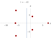
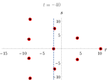
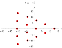
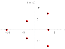
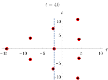
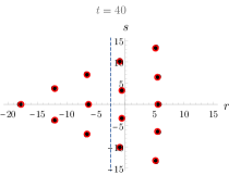
Figure 5: Triangular lump peak locations for $n=3,4,5$ at $t=-40$ (top panel) and $t=40$ (bottom panel). Total number of peaks $N={\textstyle\frac{n(n+1)}{2}}$ (see text). Black dots represent locations $z_{j}$ where $Q({\bf 0})=0$, red open circles are exact locations. Under time reversal ($t\to-t$) the peak locations are reflected across the dashed vertical line:  $r=-{\textstyle\frac{n}{2b}}$. KP parameters: $a=0,b=1$ and $\gamma_{j}=0,\,j\geq 1$.

Remark 4.1.

• It should be emphasized that (4.8) gives the approximate locations of the triangular $N$-lump solutions. The absolute difference between the exact and approximate locations is $O(|t|^{-1/3})$ when $\xi_{k}\neq 0$ and $O(|t|^{-1})$ when $\xi_{k}=0$.

• The triangular waveform patterns in KPI rational solutions were previously found in [20, 3] and more recently in [19, 14, 48] but no previous attempt was made to classify these KPI rational solutions. According to Proposition 3.3, the triangular lumps belong to Class (II) corresponding to self-conjugate partitions.

• The leading order approximate peak locations is also governed by a well known dynamical system studied in [7]. It can be shown using Lemma 4.1 (see also Remark 2.2(b)) that the wronskian $\mathop{\rm Wr}\nolimits(p_{1},p_{3},\ldots,p_{2n-1})$ is in fact a $\tau$-function $\tau(x,t)$ of the KdV equation:  $4u_{t}+6uu_{x}+u_{xxx}=0$ where the generalized Schur polynomials are redefined as $p_{n}=p_{n}(x,y,t)$ instead of $\theta_{j},\,j\geq 1$ (see Remark 2.1(b)). The corresponding rational solution of KdV is $u(x,t)=2(\ln\tau(x,t))_{xx}$ where $\tau(x,t)=(x-x_{1}(t))(x-x_{2}(t))\cdots(x-x_{N}(t))$ are the Adler-Moser polynomials [6] which are known to have distinct roots if $N=n(n+1)/2$ for some $n\in\mathbb{N}$. Plugging this form of $\tau(x,t)$ back into the KdV equation and following the method outlined in [13] one recovers the first order dynamical system for the roots $x_{j}(t)$ together with the constraints

  $$x_{jt}=\sum_{i\neq j}\frac{3}{(x_{j}-x_{i})^{2}}\,,\quad\qquad\sum_{i=1,i\neq j}^{N}\frac{1}{(x_{j}-x_{i})^{3}}=0\,,\quad j=1,2,\ldots,N\,,$$

  found in [7]. A closer examination of this dynamical system may provide further insights into the interaction properties of the triangular $N$-lump solutions but we do not pursue this matter here. Substitution of $x_{j}(t)=-({\textstyle\frac{3}{4}}t)^{1/3}\xi_{j}$ in the dynamical system and the constraints, yield

  $$\xi_{j}=-\sum_{i\neq j}\frac{12}{(\xi_{j}-\xi_{i})^{2}}\,,\quad\qquad\sum_{i=1,i\neq j}^{N}\frac{1}{(\xi_{j}-\xi_{i})^{3}}=0\,,\quad j=1,2,\ldots,N\,,$$

  which form a nonlinear system of algebraic equations that may be useful to compute the roots for the Yablonskii-Vorob’ev polynomials as well as study their properties. ‘

• Another possible interesting application of the Yablonskii-Vorob’ev polynomials is to obtain explicit formulas for the characters $\chi^{\triangle}(1^{N-3r},3^{r})$ since there is no easy algorithm to derive them in general. There are some studies which derive formulas for the coefficients $c_{r}$ of $Q_{n}(\xi)$. For example, it was shown that $c_{m-1}=0$ if $N=3m+1$ [43] and a formula for $c_{m}$ has been derived in [26], both utilize the recurrence relations for $Q_{n}(\xi)$.

4.1.2 General multi-lumps

We now consider a partition $\lambda\neq(1,2,\ldots,n)$ of $N$ and the zeros of the associated shifted Schur function $W_{\lambda}(\tilde{\theta})$ whose asymptotic form is given in (4.6). In general, $W_{\lambda}(\tilde{\theta})$ will depend on $\tilde{\theta}_{2}$. We first look for a dominant balance of the type:  $\tilde{\theta}_{1}^{N}\sim\tilde{\theta}_{1}^{N-2j}\tilde{\theta}_{2}^{j}$ which means that the corresponding character coefficient $\chi^{\lambda}(1^{N-2j},2^{j})$ has to be non-zero. To examine this possibility, it is necessary again to briefly review some ideas from partition theory. We will do so from the monograph [29] (see also the recent work [9]).

Murnaghan-Nakayama rule and 2-core of a partition:  A combinatorial way of computing the character $\chi^{\lambda}(1^{N-2j},2^{j})$ of the symmetric group $S_{N}$ is to recursively apply the Murnaghan-Nakayama rule which for the present purpose reads as follows

$$\chi^{\lambda}(1^{N-2j},2^{j})=\sum_{\mu\subset\lambda}(-1)^{ht(S)}\chi^{\mu}(1^{N-2j},2^{j-1})\,,$$

where the sum is over all partitions $\mu\subset\lambda$ such that $S=\lambda/\mu$ is either a vertical or horizontal 2-block, i.e. either $Y_{\lambda/\mu}=\raisebox{3.61371pt}{\ytableausetup{boxsize=0.4em}\ydiagram{1,1}}\,,$ or $Y_{\lambda/\mu}=\ytableausetup{boxsize=0.5em}\ydiagram{2}\,,$ and $ht(S)=\#$ of rows in $S$ minus 1. Thus $ht(S)=1$ for a vertical 2-block and $ht(S)=0$ for a horizontal one. Successive applications of the Murnaghan-Nakayama rule can exhaust all the 2-cycles, which leads to a form

$$\chi^{\lambda}(1^{N-2j},2^{j})=\sum_{\rho}\pm\chi^{\rho}(1^{N-2j})\,,$$

where $\rho\subset\lambda$ are partitions whose diagrams $Y_{\rho}$ are obtained by peeling off $j$ 2-blocks from $Y_{\lambda}$. The parity $\pm$ depends on the number of horizontal and vertical 2-blocks peeled away during the process of obtaining a specific $Y_{\rho}$ starting from $Y_{\lambda}$, and the sum is over all possible partitions $\rho$ whose diagram $Y_{\rho}$ consists of $N-2j$ boxes. The character $\chi^{\rho}(1^{N-2j})\neq 0$ is known since it is the dimension of the irreducible representation $\rho$. Note that if $\rho=\emptyset,\,\chi^{\emptyset}=1$. However, this reduction process may lead to obstructions where a stage is reached when the resulting partition $\tilde{\lambda}$ is such that no more 2-blocks can be peeled away from $\tilde{\lambda}$ and the recursive process has to prematurely terminate. The partition $\tilde{\lambda}$ is called the 2-core of the partition $\lambda$. It can be shown that 2-cores are precisely triangular partitions discussed in Section 4.1.1. The key ingredient of this process is to peel off one 2-block at a time so that the resulting diagram is still a Young diagram of some partition $\mu\subset\lambda$. The terminating 2-core partition $\tilde{\lambda}$ is always the same no matter which path is followed. Moreover the parity $\pm$ which depends on the number of vertical 2-blocks removed along a path is also invariant across all paths. Thus there exists a positive integer $q$ such that the character coefficient $\chi^{\lambda}(1^{N-2q},2^{q})$ of $\tilde{\theta}_{1}^{N-2q}\tilde{\theta}_{2}^{q}$ of the Schur function $W_{\lambda}$ in (4.6) takes the form

$$\chi^{\lambda}(1^{N-2q},2^{q})=\pm N(\lambda,\tilde{\lambda})\chi^{\tilde{\lambda}}(1^{N-2q})=C(\lambda,\tilde{\lambda})\neq 0$$

for some triangular partition $\tilde{\lambda}$ and where $N(\lambda,\tilde{\lambda})$ is the total number of possible paths from $Y_{\lambda}$ to $Y_{\tilde{\lambda}}$. The expression for $C(\lambda,\tilde{\lambda})$ is given in [9]. More important for our discussion is the fact that then $\chi^{\lambda}(1^{N-2q-2},2^{q+1})=0$ since after removing $q$ 2-blocks the 2-core $\tilde{\lambda}$ is reached. The example below illustrates the process.

Example 4.2.

Let $\lambda=(1,1,3,4)$. All possible sequences of peeling off a vertical or a horizontal 2-block starting from $Y_{\lambda}$ and the intermediate diagrams $Y_{\mu}$ are shown below. Finally all (3) possible paths indicated by the arrows terminate at the Young diagram $Y_{\tilde{\lambda}}=\raisebox{3.61371pt}{\ytableausetup{boxsize=0.5em}\ydiagram{2,1}}$ at the lower right corner, which corresponds to a triangular partition.

$$\begin{matrix}\raisebox{7.22743pt}{\ytableausetup{boxsize=0.6em}\ydiagram{4,3,1,1}}&\longrightarrow&\raisebox{7.22743pt}{\ytableausetup{boxsize=0.6em}\ydiagram{4,1,1,1}}&\longrightarrow&\raisebox{7.22743pt}{\ytableausetup{boxsize=0.6em}\ydiagram{2,1,1,1}}\\ \big{\downarrow}&&\big{\downarrow}&&\downarrow\\ \ytableausetup{boxsize=0.6em}\ydiagram{4,3}&\longrightarrow&\ytableausetup{boxsize=0.6em}\ydiagram{4,1}&\longrightarrow&\ytableausetup{boxsize=0.6em}\ydiagram{2,1}\end{matrix}$$

Notice that along each path 1 vertical and 2 horizontal 2-blocks are removed to arrive at $Y_{\tilde{\lambda}}$ before the process terminates. Thus, $\chi^{(1,1,3,4)}(1^{3},2^{3})=-3\chi^{(1,2)}(1^{3})$ but $\chi^{(1,1,3,4)}(1,2^{4})=0$ since no further 2-blocks can be peeled off from the diagram $Y_{\tilde{\lambda}}$.

It is also possible to determine the positive integer $q$ which is the maximum number of 2-blocks removed from $Y_{\lambda}$, precisely as follows. Let $m=(m_{1},\ldots,m_{n}),\,1\leq m_{1}<\dots<m_{n}$ be the degree vector of a partition $\lambda$ of $N\in\mathbb{N}$. After removing a 2-block, one arrives at an (unordered) sequence $(m_{1},\ldots,m_{j}-2,\ldots,m_{n})$ for some $1\leq j\leq n$. After rearranging the resulting sequence in ascending order, yields the sequence $m^{\prime}$ which is the degree vector of a new partition $\mu$ so long as the components of $m^{\prime}$ are all distinct and non-negative. Thus, the terminal 2-core $\tilde{\lambda}$ partition is reached when the successive components of the corresponding degree vector $\tilde{m}$ differ by at most 2. Next consider the initial degree vector $m$ as an unordered set which is a union of $k$ odd and $l$ even positive integers with $k+l=n$. After removing all possible 2-blocks from the odd set, the residual set is $\{1,3,\ldots,2k-1\}$ while the residual even set becomes $\{0,2,\ldots,2l-2\}$. Let us assume $k>l$. Then after rearranging the union of these residual sets in ascending order one recovers the degree vector $\tilde{m}=(0,1,\ldots,2l-2,2l-1,2l+1,\ldots 2k-1\}$ corresponding to the 2-core

$$\tilde{\lambda}=(\underbrace{0,0,\ldots,0}_{2l},\underbrace{1,3,\ldots,d}_{k-l})$$

of length $l(\tilde{\lambda})=d=k-l$, using the relation $\tilde{\lambda}_{j}=\tilde{m}_{j}-j+1$. $\tilde{\lambda}$ is a triangular partition of size $|\tilde{\lambda}|={\textstyle\frac{d(d+1)}{2}}$. The total number of 2-blocks removed is

$$q={\textstyle\frac{1}{2}}(|\lambda|-|\tilde{\lambda}|)\,,\quad\text{since}\quad|\lambda|-|\tilde{\lambda}|=(m_{1}+\cdots+m_{n})-(1+\cdots+2k-1)-(2+\cdots+2l-2)$$

is an even number. If $k<l$ then a similar argument shows that $d=l-k-1$, and if $k=l$ then $d=0$.

Example 4.3.

For $\lambda=(1,1,3,4)$ as in Example 4.2, the degree vector $m=(1,2,5,7)$ where $m_{2}=2$ is even and the remaining 3 components are odd. Then $\{2\}\cup\{1,5,7\}\to\{0\}\cup\{1,3,5\}$ after removing $(2-0)+(1-1)+(5-3)+(7-5)=6$ boxes from $Y_{\lambda}$. So $q=3$. The degree vector for the core partition is $\tilde{m}=(0,1,3,5)$ so that $\tilde{\lambda}=(0,0,1,2)$ and $d=k-l=3-1=2$.

We conclude our brief excursion to partition theory with the following.

Proposition 4.1.

Let $\lambda\neq(1,2,\ldots,n)$ be a non-triangular partition of $N\in\mathbb{N}$. Suppose the degree vector of $\lambda$ has $k$ odd and $l$ even components, $k+l=n$. Then there exists a largest positive integer $q\leq\lfloor{\textstyle\frac{N}{2}}\rfloor$ such that the character coefficient $\chi^{\lambda}(1^{N-2q},2^{q})\neq 0$ in the associated Schur function $W_{\lambda}(\theta)$. The integer $q={\textstyle\frac{N-|\tilde{\lambda}|}{2}}$ where the $n$-tuple $\tilde{\lambda}=(0,\dots,0,1,2,\ldots,d)$ is the 2-core of $\lambda$ and $d=k-l$ if $k\geq l$ and $d=l-k-1$ if $l>k$. Hence, $N-2q=|\tilde{\lambda}|={\textstyle\frac{d(d+1)}{2}}$. Furthermore, the coefficient of $\theta_{2}^{q}$ in $W_{\lambda}(\theta)$ is $C_{q}W_{\tilde{\lambda}}(\theta)$ for some constant $C_{q}$ that determines the value of $\chi^{\lambda}(1^{N-2q},2^{q})$.

The last part of Proposition 4.1 will be explained later in more details. The first part of Proposition 4.1 implies the dominant balance $\tilde{\theta}_{1}^{N}\sim\tilde{\theta}_{1}^{N-2q}\tilde{\theta}_{2}^{q}$ in (4.5) so that $\tilde{\theta}_{1}\sim|t|^{1/2},\,|t|\gg 1$. Collecting all the dominant terms that are of the form $\tilde{\theta}_{1}^{N-2j}\tilde{\theta}_{2}^{j}\sim O(|t|^{N/2})$ from (4.6), yields

$$W_{\lambda}(\tilde{\theta})\sim\sum_{j=0}^{q}\chi^{\lambda}(1^{N-2j},2^{j})\frac{\tilde{\theta}_{1}^{N-2j}\tilde{\theta}_{2}^{j}}{(N-2j)!j!}=\mathop{\rm Wr}\nolimits(p_{m_{1}},\ldots,p_{m_{n}})\,,$$ (4.9)

where $p_{r}=p_{r}(\tilde{\theta}_{1},\tilde{\theta}_{2},0)$ in the above wronskian. From (2.16), $\tilde{\theta}_{1}=iz$ where $z=(r+h_{1}+is+\gamma_{1})$ and $\tilde{\theta}_{2}=\frac{is}{2b}-3bt+h_{2}+\gamma_{2}$. Proceeding similarly as in Section 4.1.1, one rescales $z=|t|^{1/2}\xi$, and uses (2.4) to obtain

$$p_{r}(\tilde{\theta}_{1},\tilde{\theta}_{2},0)\sim i^{r}|t|^{r/2}\big{(}H_{r}(\xi,\eta)+O(|t|^{-1/2})\big{)}\,.$$

The heat polynomials $H_{r}(\xi,\eta)$ and their generating function are obtained directly from (2.4) and (2.3)

$$H_{r}(\xi,\eta)=\sum_{j,k\geq 0}\frac{\xi^{j}\eta^{k}}{j!k!},\quad j+2k=r\,,\qquad\exp(\alpha\xi+\alpha^{2}\eta)=\sum_{r=0}^{\infty}H_{r}(\xi,\eta)\alpha^{r}\,,\quad\quad\eta=\left\{\begin{matrix}3b\,,&\quad t\geq 0\vspace{0.05 in}\\ -3b\,,&\quad t<0\end{matrix}\right.\,.$$

These heat polynomials $H_{r}(\xi,\eta)$ were also introduced recently in order to investigate a special family of KPI lumps [10]. Substituting the asymptotic expression of $p_{r}$ into (4.9) leads to

$$W_{\lambda}(r,s,t)\sim i^{N}|t|^{N/2}\big{[}H_{\lambda}(\xi,\eta)+O(|t|^{-1/2})\big{]}\,,$$ (4.10a)

where $$H_{\lambda}(\xi,\eta)$$ is the wronskian of the heat polynomials given by

$$H_{\lambda}(\xi,\eta)=\mathop{\rm Wr}\nolimits(H_{m_{1}},\ldots,H_{m_{n}})=\xi^{N-2q}\sum_{j=0}^{q}\frac{\chi^{\lambda}(1^{N-2j},2^{j})}{(N-2j)!j!}\,\xi^{2(q-j)}\eta^{j}\,,$$ (4.10b)

and the positive integer $$q$$ is defined in Proposition 4.1.

The heat polynomials $H_{r}(\xi,\eta)$ above can be normalized to the Hermite polynomials (see Remark 4.2(b)) so that the polynomials $H_{\lambda}$ are related to the wronskian of Hermite polynomials after certain rescalings. The wronskian of Hermite polynomials arise in the study of the Schrödinger equation:  $\psi^{\prime\prime}(z)=(u(z)-\lambda)\psi(z)$ where $u(z)$ is rational, growing as $z^{2}$ at infinity, and $\psi(z)$ is single-valued in the complex $z$-plane for all $\lambda\in\mathbb{C}$ [35].

Treating $H_{\lambda}$ as a polynomial in $\xi$ only, and $\eta=\pm 3b$ as a parameter, it is clear that $H_{\lambda}(\xi)$ is of degree $N$ and has a root at $\xi=0$ with multiplicity $N-2q$. It is conjectured that the non-zero roots of $H_{\lambda}(\xi)$ are simple [16] and will be assumed to be true in what follows. Furthermore, since $\xi^{2q-N}H_{\lambda}(\xi)$ in (4.10b) is a polynomial in $\xi^{2}$ of degree $q$ with real coefficients, the remaining non-zero roots admit the following symmetries:  (a)  if $\xi_{j}\in\mathbb{C}$, then the quartet $\{\pm\xi_{j},\pm\bar{\xi}_{j}\}$, and (b)  if $\xi_{j}\in\mathbb{R}$, then the pair $\pm\xi_{j}$ are all roots of $H_{\lambda}(\xi)$. Another symmetry stems from the dependence of the roots on the parameter $\eta$. It is evident from the definition of the heat polynomials $H_{r}(\xi,\eta)$ given above (4.10a) that $H_{r}(\xi,-\eta)=i^{r}H_{r}(-i\xi,\eta)$ which implies that $H_{\lambda}(\xi,-\eta)=i^{N}H_{\lambda}(-i\xi,\eta)$ and its roots satisfy $\xi_{j}(\eta=-3b)=i\xi_{j}(\eta=3b)$.

When $\xi_{j}\neq 0$, by putting $W_{\lambda}(r,s,t)=0$ in (4.10a) and solving asymptotically for

$$z(t)=|t|^{1/2}(z_{0}+\epsilon z_{1}+\epsilon^{2}z_{2}+\cdots)\,,\qquad\epsilon=|t|^{-1/2}$$

like in the triangular $N$-lump case, one obtains the $2q$ approximate peak locations for the general $N$-lump solutions when $|t|\gg 1$ in terms of the roots of $H_{\lambda}(\xi)$. Denoting the peak locations by $Z^{\pm}_{j}=r^{\pm}_{j}+is^{\pm}_{j}$ corresponding to positive and negative $t$ respectively, one obtains for $|t|\gg 1$,

$$Z^{\pm}_{j}(t)=(r_{0}-{\textstyle\frac{n}{2b}}+is_{0})+|t|^{1/2}\big{[}\xi_{j}(\eta=\pm 3b)+O(|t|^{-1/2})\big{]}\,,\quad j=1,2,\ldots,2q\,,$$ (4.11)

where as usual, $h_{1}={\textstyle\frac{n}{2b}}$ from (4.4) and $-\gamma_{1}=r_{0}+is_{0}$. Furthermore, $(r^{+}_{j}(t),s^{+}_{j}(t))\sim(-s^{-}_{j}(t),r^{-}_{j}(t))$ as $|t|\to\infty$ due to the symmetry of the roots:  $\xi_{j}(\eta=-3b)=i\xi_{j}(\eta=3b)$. The surface wave pattern due to the peak locations in the $rs$-plane are markedly different from those of the triangular $N$-lumps due to the quartet or doublet root patterns of $H_{\lambda}(\xi)$ as shown below in Figure 6. Also, unlike in (4.8), the $O(1)$ term in (4.11) will change if $z_{1}\neq 0$ in the asymptotic expansion of $z(t)$ above. Further details of this asymptotics will not be pursued in this paper.

Example 4.4.

Consider the partition $\lambda=(3,3)$ with $m=(3,4)$ where $N=6$. The Schur function is given by

$$W_{\lambda}=\begin{vmatrix}p_{3}&p_{4}\\ p_{2}&p_{3}\end{vmatrix}=\frac{\tilde{\theta}_{1}^{6}}{144}+\frac{\tilde{\theta}_{1}^{4}\tilde{\theta}_{2}}{24}+\frac{\tilde{\theta}_{1}^{2}\tilde{\theta}_{2}^{2}}{4}-\frac{\tilde{\theta}_{2}^{3}}{2}-\frac{\tilde{\theta}_{1}^{3}\tilde{\theta}_{3}}{6}+\tilde{\theta}_{1}\tilde{\theta}_{2}\tilde{\theta}_{3}-(\frac{\tilde{\theta}_{1}^{2}}{2}-\tilde{\theta}_{2})\tilde{\theta}_{4}\,,$$

after using (2.4). The first four terms above are dominant consistent with the scaling $\tilde{\theta}_{1}=i|t|^{1/2}\xi$, and leads to

$$W_{\lambda}\sim i^{6}|t|^{3}\big{[}H_{\lambda}(\xi,\eta)+O(|t|^{-1/2}\big{]}\,,\quad H_{\lambda}=\mathop{\rm Wr}\nolimits(H_{3},H_{4})=\frac{1}{144}\big{(}\xi^{6}+6\xi^{4}\eta+36\xi^{2}\eta^{2}-72\eta^{3}\big{)}\,,$$

as in (4.10a). Note that $\xi=0$ is not a root of $H_{\lambda}$ as $q=N/2=3$ in (4.10b). Since $\eta=3b$ for positive $t$, setting $w={\textstyle\frac{\xi^{2}}{3b}}$ it can be easily verified that the resulting cubic polynomial $w^{3}+6w^{2}+36w-72$ has a single real root that is positive and a pair of complex conjugate roots. Consequently, 4 of the 6 distinct zeros of $H_{\lambda}(\xi)$ arise in complex conjugate pairs, and remaining 2 are real which corresponds to the positive real root of the cubic polynomial in $w$. The approximate peak locations given by (4.11) in this case are shown in the right panel of Figure 6. By using the symmetry $\xi_{j}(\eta=-3b)=i\xi_{j}(\eta=3b)$ of the zeros of $H_{\lambda}(\xi,\eta)$ one obtains the leading order approximate peak locations for $t<0$. These are shown in the left panel of Figure 6 confirming that $(r^{+}_{j}(t),s^{+}_{j}(t))\sim(-s^{-}_{j}(t),r^{-}_{j}(t))$ for $|t|\gg 1$.

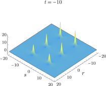
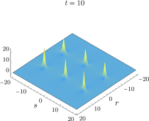
Figure 6: The $6$-lump solutions of Example 4.4. Solutions corresponding to $t=-10$ (left panel) and $t=10$ (right panel). KP Parameters:  $a=0,b=1,\,\gamma_{j}=0,\,j\geq 1$.

Yet another interesting result concerns the relation between the asymptotic peak locations of a pair of class (I) $N$-lump solutions in Section 3.2 corresponding to partition $\lambda$ and its conjugate $\lambda^{\prime}$. This relationship occurs when the approximate peak locations are given by (4.11) corresponding to the non-zero roots of $H_{\lambda}$ and $H_{\lambda^{\prime}}$. Applying the first involution relation in (3.5) to (4.9) yields $W_{\lambda^{\prime}}(\tilde{\theta}_{1},\tilde{\theta}_{2})=W_{\lambda}(\tilde{\theta}_{1},-\tilde{\theta}_{2})$. From $\tilde{\theta}_{2}=\frac{is}{2b}-3bt+h_{2}+\gamma_{2}$ and the fact that $s\sim O(|t|^{1/2})$ (since $\theta_{1}\sim O(|t|^{1/2}))$ it follows that $\tilde{\theta}_{2}(-t)\sim-\tilde{\theta}_{2}(t)$ for $|t|\gg 1$. Hence, one obtains the leading order asymptotic relation $W_{\lambda^{\prime}}(r,s,t)\sim W_{\lambda}(r,s,-t)$ in (4.10a). Consequently, the asymptotic peak locations given by (4.11) for the $N$-lump solutions corresponding to partitions $\lambda$ and $\lambda^{\prime}$ satisfy

$$Z^{\lambda^{\prime}}_{j}(t)\sim Z^{\lambda}_{j}(-t)\,,\quad j=1,\ldots,2q\,,\qquad|t|\gg 1\,.$$

In this context, one should note that the 2-core partition $\tilde{\lambda}$ is the same for both $\lambda$ and its conjugate $\lambda^{\prime}$ since removing a horizontal 2-block from $\lambda$ is equivalent to removing a vertical 2-block from $\lambda^{\prime}$ and vice-versa. Hence it follows from Proposition 4.1 that the positive integer $q$ in (4.9) is the same for both Schur functions $W_{\lambda}$ and $W_{\lambda^{\prime}}$. Note that the involution in (3.5) can be applied directly to obtain the relation $H_{\lambda^{\prime}}(\xi,\eta)=H_{\lambda}(\xi,-\eta)$ reported in [16, 9].

When $\xi=0$ is a root of $H_{\lambda}(\xi)$ with multiplicity $N-2q$, the $N-2q$ peak locations are not separated to leading order at the $O(|t|^{1/2})$ time scale. It is then necessary to examine the terms that were subdominant in (4.6) when $\tilde{\theta}_{1}\sim|t|^{1/2}$ and were neglected to obtain (4.9). Looking back in (4.6) such terms that are significant for $|t|\gg 1$ are of the form $\tilde{\theta}_{1}^{k}\tilde{\theta}_{2}^{q}\tilde{\theta}_{3}^{l},\,k+3l=N-2q$ where the exponent of $\tilde{\theta}_{2}$ is fixed at its largest value $q$. In other words, one needs to collect the coefficient of $\tilde{\theta}_{2}^{q}$ from the Schur function $W_{\lambda}(\tilde{\theta})$ in (4.6). For this purpose we split $\tilde{\theta}=\hat{\theta}+\delta$ where $\hat{\theta}=(\tilde{\theta}_{1},0,\tilde{\theta}_{3},\ldots)+(0,\tilde{\theta}_{2},0,\ldots)$ and apply (4.2) to $W_{\lambda}(\tilde{\theta})$, which leads to the following

$$W_{\lambda}(\hat{\theta}+\delta)=\sum_{\mu}W_{\mu}(\hat{\theta})W_{\lambda/\mu}(\delta)\,,\qquad\mu\subseteq\lambda\,.$$

It can be shown from the definition of $W_{\lambda/\mu}$ in (3.1) that since $\delta$ depends only on $\tilde{\theta}_{2}$, $W_{\lambda/\mu}(\delta)$ is nonvanishing only when $\mu$ is obtained from $\lambda$ by removing successive 2-blocks, i.e., $|\lambda|-|\mu|=2j,\,j\geq 0$ so that $W_{\lambda/\mu}(\delta)=C_{j}\tilde{\theta}_{2}^{j}$ for some constant $C_{j}$. This is precisely the process of obtaining the 2-core partition of $\lambda$ as explained at the beginning of this subsection (see also Example 4.2). Therefore, the above sum starting from $\mu=\emptyset$ must terminate when $\mu=\tilde{\lambda}$ which is the 2-core of $\lambda$ and $W_{\lambda/\tilde{\lambda}}(\delta)=C_{q}\tilde{\theta}_{2}^{q}$ as claimed at the end of Proposition 4.1. Since $\tilde{\lambda}$ is a triangular partition the analysis presented in Section 4.1.1 applies to this case. Using (3.1) and the degree vector $\tilde{m}=(0,1,\ldots,2l-2,2l-1,2l+1,\ldots 2k-1\}$ for the partition $\tilde{\lambda}$ in Proposition 4.1, one obtains

$$W_{\tilde{\lambda}}(\hat{\theta})=\mathop{\rm Wr}\nolimits(p_{0},p_{1},\ldots,p_{2l-1},p_{2l+1},\ldots,p_{2k-1})=\mathop{\rm Wr}\nolimits(p_{1},p_{3},\ldots,p_{2d-1})\,,\qquad d=k-l\,,\quad k\geq l\,.$$

A similar expression can be obtained when $k<l$. Also when $k=l,\,d=0$, and $\tilde{\lambda}=\emptyset$. In this case, $N$ is even and $q=N/2$ so that $\xi=0$ is not a root of $H_{\lambda}(\xi)$ (cf. Example 4.4).

Isolating the coefficient of $\tilde{\theta}_{2}^{q}$ in $W_{\lambda}(\tilde{\theta})$ leads to the dominant behavior

$$W_{\lambda}(\tilde{\theta})\sim W_{\lambda/\tilde{\lambda}}(\delta)W_{\tilde{\lambda}}(\hat{\theta})=C_{q}\tilde{\theta}_{2}^{q}\mathop{\rm Wr}\nolimits(p_{1},p_{3},\dots,p_{2d-1})\,,$$ (4.12)

and when $W_{\lambda}(\tilde{\theta})=0$ the corresponding dominant balance is $\tilde{\theta}_{1}\sim O(|t|^{1/3})$ as in Section 4.1.1. In this case, when $|t|\gg 1$, $W_{\lambda}(\tilde{\theta})\sim O(|t|^{(N+q)/3})$ while the terms in (4.9), $\tilde{\theta}_{1}^{N-2j}\tilde{\theta}_{2}^{j}\sim O(|t|^{(N+j)/3})$ for $j<q$, are now sub-dominant. Then the remaining $d=N-2q$ approximate peak locations for the $N$-lump solution corresponding to partition $\lambda$ as well as its conjugate $\lambda^{\prime}$ are obtained by zeros of the Yablonskii-Voro’bev polynomial $Q_{d}(\xi)$ as in (4.8) for $j=1,\ldots,d$. Also note that the coefficient $C_{q}$ in (4.12) is recovered from $W_{\lambda/\tilde{\lambda}}(\delta)$. Indeed from (3.1),

$$C_{q}\tilde{\theta}_{2}^{q}=W_{\lambda/\tilde{\lambda}}(\delta)=\det(p_{m_{j}-\tilde{m}_{i}})(\delta)\,,\qquad\delta=(0,\tilde{\theta}_{2},0,\ldots)\,,$$ (4.13)

where $m,\tilde{m}$ denote the degree vectors of the partitions $\lambda,\tilde{\lambda}$, respectively.

In summary, it is established that there are indeed $N$ distinct peaks for the general $N$-lump solutions of KPI equation (1.1). The wave pattern in the $rs$-plane exhibit two distinct time scales such that the dynamics of $q$ out of the $N$ peaks occurs at a faster $O(|t|^{1/2})$ time scale, while the remaining $N-2q$ peaks evolve at a slower $O(|t|^{1/3})$ time scale. Consequently, the $q$ peaks in the far field region of the wave pattern form a rectangular shape or lie symmetrically along the $r$- or $s$-axis, whereas the other $N-2q$ peaks form a triangular pattern in the near-field region of the $rs$-plane.

Example 4.5.

Let $\lambda=(1,4)$ corresponding to $m=(1,5)$ and $N=5$. Then the Schur function from (4.3) is

$$W_{\lambda}(\tilde{\theta})=\mathop{\rm Wr}\nolimits(p_{1},p_{5})=\frac{\tilde{\theta}_{1}^{5}}{30}+\frac{\tilde{\theta}_{1}^{3}\tilde{\theta}_{2}}{3}+\frac{\tilde{\theta}_{1}^{2}\tilde{\theta}_{3}}{2}-\tilde{\theta}_{2}\tilde{\theta}_{3}-\tilde{\theta}_{5}\,.$$

The largest exponent of $\tilde{\theta}_{2}$ in $W_{\lambda}(\tilde{\theta})$ is $q=1$. So the first dominant balance $\tilde{\theta}_{1}^{5}\sim\tilde{\theta}_{1}^{3}\tilde{\theta}_{2}$ to solve (4.5) gives the scaling $\tilde{\theta}_{1}\sim|t|^{1/2}$, Collecting the dominant terms which are $O(|t|^{5/2})$, one obtains as in (4.9) $W_{\lambda}\sim{\textstyle\frac{\tilde{\theta}_{1}^{3}}{30}}(\tilde{\theta}_{1}^{2}+\tilde{\theta}_{2}$), the rest of the terms in $W_{\lambda}$ are subdominant being $O(|t|^{2})$. Next putting $\tilde{\theta}_{1}=iz,\,z=|t|^{1/2}\xi$, and after using (2.16) for $\tilde{\theta}_{1},\tilde{\theta}_{2}$, the dominant terms give the following asymptotics accordingly as (4.10b)

$$W_{\lambda}\sim i^{5}|t|^{5/2}\big{[}H_{\lambda}(\xi,\eta)+O(|t|^{-1/2})\big{]}\,,\quad\qquad H_{\lambda}(\xi,\eta)=\mathop{\rm Wr}\nolimits(H_{1},H_{5})=\frac{\xi^{3}}{30}\big{(}\xi^{2}+10\eta\big{)}\,.$$

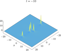
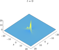
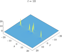
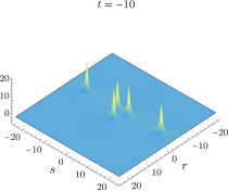
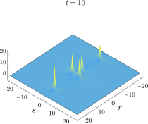
Figure 7: The $5$-lump solutions of Example 4.4. Solutions corresponding to $\lambda=(1,4)$ (top panel) and the conjugate $\lambda^{\prime}=(1,1,1,2)$ (bottom panel). Note that the two peaks in the outer region of the plane satisfy the symmetry $Z^{\lambda^{\prime}}_{j}(t)\sim Z^{\lambda}_{j}(-t)$ at $t=\pm 10$. A triangular configuration of three lumps are formed in the inner region which is the same for both $\lambda$ and $\lambda^{\prime}$. KP Parameters: same as in Figure 6.

The approximate peak locations for $|t|\gg 1$ are obtained by solving $W_{\lambda}=0$ for $z(t)=|t|^{1/2}(z_{0}+\epsilon z_{1}+\cdots)$ where $\epsilon=|t|^{-1/2}$. Hence, to leading order the distinct peak locations $z_{0}$ in this example correspond to the two non-zero roots $\xi=\pm\sqrt{-10\eta}$ of $H_{\lambda}(\xi)$ above. Using $\eta=\pm 3b$ and the shift from (4.4) $h_{1}={\textstyle\frac{n}{2b}}={\textstyle\frac{1}{b}}$ (since $n=2$ here), the approximate peak locations for $|t|\gg 1$ are given by

$$r^{\pm}(t)+is^{\pm}(t)=(r_{0}-{\textstyle\frac{1}{b}}+is_{0})+|t|^{1/2}\big{(}\sqrt{\mp 30b}+O(|t|^{-1/2})\big{)}\,,\qquad-\gamma_{1}=r_{0}+is_{0}\,,$$

as in (4.11). When $t<0$, $\eta=-3b$ corresponds to real roots $\xi=\pm\sqrt{30b}$. Hence for $t<0$ and $|t|\gg 1$, the two peaks lie on the $r$-axis symmetrically about the origin. For $t\gg 1$, the two peaks are instead located on the $s$-axis symmetrically about the origin consistent with the symmetry $(r^{+}_{j}(t),s^{+}_{j}(t))\sim(-s^{-}_{j}(t),r^{-}_{j}(t))$ as $|t|\to\infty$. These features are illustrated in Figure 8. From the asymptotic expansion of $z(t)$, one can also calculate $z_{1}$ which has a further $O(1)$ contribution to the peak locations. For example, when $t\gg 1$, $z_{1}={\textstyle\frac{11}{5b}}$ which shifts the two peak locations slightly to the right of the $s$-axis. This effect is evident in the top right panel of Figure 8.

The remaining approximate peak locations are obtained from a second dominant balance $\tilde{\theta}_{1}\sim O(|t|^{1/3})$ in $W_{\lambda}(\tilde{\theta})$ above, arising from the terms linear in $\tilde{\theta}_{2}$. That is, $W_{\lambda}(\tilde{\theta})\sim\tilde{\theta}_{2}(\tilde{\theta}_{1}^{3}/3-\tilde{\theta}_{3})\sim O(|t|^{2})$, and the remaining terms are then $O(|t|^{5/3})$, hence subdominant. Solving for $\tilde{\theta}_{1}^{3}/3-\tilde{\theta}_{3}\sim 0$, and using (4.4) with $n=2$ leads to the approximate peak locations that are exactly the same as the ones for the $3$-lump solution given above Figure 4 of Section 2.3.3. The origin of the second dominant balance is from the 2-core $\tilde{\lambda}=(1,2)$ of the partition $\lambda=(1,4)$ obtained by removing a single horizontal 2-block from its Young diagram i.e., $Y_{\lambda}=\raisebox{3.61371pt}{\ytableausetup{boxsize=0.4em}\ydiagram{4,1}}\longrightarrow\raisebox{3.61371pt}{\ytableausetup{boxsize=0.4em}\ydiagram{2,1}}=Y_{\tilde{\lambda}}$. Since $m_{1},m_{2}$ are both odd, $d=k-l=2$ from Proposition 4.1. Then $|\tilde{\lambda}|={\textstyle\frac{d(d+1)}{2}}=3$. Again from Proposition 4.1, $N-2q=|\tilde{\lambda}|=3$ implies that $q=1$ which has already been found as the largest exponent of $\tilde{\theta}_{2}$ in $W_{\lambda}(\tilde{\theta})$ above. Using (4.12) one can directly obtain the dominant term $W_{\lambda}(\tilde{\theta})\sim C_{1}\tilde{\theta}_{2}\mathop{\rm Wr}\nolimits(p_{1},p_{3})=C_{1}\tilde{\theta}_{2}(\tilde{\theta}_{1}^{3}/3-\tilde{\theta}_{3})$. The coefficient $C_{1}$ is obtained by applying (4.13). Here $m=(1,5)$ and $\tilde{m}=(1,3)$. Hence, $C_{1}\tilde{\theta}_{2}=\big{|}\begin{smallmatrix}p_{0}&p_{4}\\ 0&p_{2}\end{smallmatrix}\big{|}=p_{2}(0,\tilde{\theta}_{2})=\tilde{\theta}_{2}\Rightarrow C_{1}=1$. The full wave pattern as well as the peak locations in the $rs$-plane are illustrated in the top panels of Figures 7 and  8.

Let us also briefly consider the the $5$-lump solution corresponding to the conjugate partition $\lambda^{\prime}=(1,1,1,2)$ with degree vector $m^{\prime}=(1,2,3,5)$. By direct computation one verifies that

$$W_{\lambda^{\prime}}(\tilde{\theta})=\mathop{\rm Wr}\nolimits(p_{1},p_{2},p_{3},p_{5})=\frac{\tilde{\theta}_{1}^{5}}{30}-\frac{\tilde{\theta}_{1}^{3}\tilde{\theta}_{2}}{3}+\frac{\tilde{\theta}_{1}^{2}\tilde{\theta}_{3}}{2}+\tilde{\theta}_{2}\tilde{\theta}_{3}-\tilde{\theta}_{5}\,,$$

which also follows from the first involution relation in (3.5) by simply switching $\tilde{\theta}_{2}\to-\tilde{\theta}_{2}$ in $W_{\lambda}(\tilde{\theta})$ above. Therefore, again $q=1$ and the dominant balances are same as before. However, when $\tilde{\theta}_{1}\sim O(|t|^{1/2})$,

$$W_{\lambda^{\prime}}\sim i^{5}|t|^{5/2}\big{[}H_{\lambda^{\prime}}(\xi,\eta)+O(|t|^{-1/2})\big{]}\,,\quad\qquad H_{\lambda^{\prime}}(\xi,\eta)=H_{\lambda}(\xi,-\eta)=i^{N}H_{\lambda}(i\xi,\eta)\,,$$

so that the real and pure imaginary roots are switched from the previous case. This leads to the symmetry $Z_{j}^{\lambda^{\prime}}(t)\sim Z_{j}^{\lambda}(-t),\,\,j=1,2$ when $|t|\gg 1$ for the two peaks located in far field region of the $rs$-plane. However, the approximate configuration of the remaining three peaks that form the inner core in the near field region remains the same as in the previous case. Note that in this case $n=4$ so that the shift $h_{1}={\textstyle\frac{2}{b}}$ is larger than the previous case. This causes the peak locations to shift further toward the left of the $s$-axis as clearly evident from e.g., the bottom left frame in Figure 8. The full wave pattern and the peak locations are shown in the bottom panels of Figures 7 and  8.

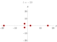
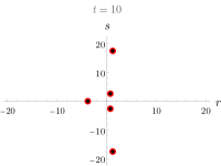
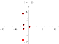
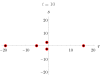
Figure 8: Peak locations for Example 4.4 at $t=-10$ (left frames) and $t=10$ (right frames). Black dots represent approximate peak locations where $Q({\bf 0})=0$ as in (4.5), red open circles are exact locations. The top panel shows $5$-lump peak locations associated with the partition $\lambda=(1,4)$, the bottom panel corresponds to its conjugate partition. KP parameters: same as in Figure 7.

Remark 4.2.

• It should be emphasized that (4.11) assumes that the non-zero roots of the polynomial $H_{\lambda}(\xi)$ are simple. Our assumption is based on a conjecture made in [16] and we are yet to find a counter-example.

• The heat polynomials $H_{n}(\xi,\eta)$ introduced above (4.10a) satisfies the heat equation $h_{\xi\xi}=h_{\eta}$ in two-dimensions with initial condition $h(\xi,0)={\textstyle\frac{\xi^{n}}{n!}}$. They are closely related to the Hermite polynomials via $H_{n}(\xi,\eta)={\textstyle\frac{(-\eta)^{n/2}}{n!}}\,H_{n}(z),\,\,z=\xi(-4\eta)^{-1/2}$. The roots of the heat polynomials $H_{n}(\xi,\eta)$ are real (in $\xi$) if the parameter $\eta<0$ and pure imaginary if $\eta>0$. These roots describe the approximate peak locations of $N$-lump solutions of KPI when the associated partition $\lambda$ has only one part, i.e., $n=1$ and $\lambda=(N)$. These were recently studied in [10].

• The coefficient $C_{q}$ in Proposition 4.1 is related to the character $\chi^{\lambda}(1^{N-2q},2^{q})$ by the formula

  $$C_{q}=\frac{\chi^{\lambda}(1^{N-2q},2^{q})}{\chi^{\tilde{\lambda}}(1^{N-2q})q!}\,.$$

  An expression for $C_{q}$ was derived in [9] using the same ideas related to the 2-core of a partition as the present article. However, we believe that (4.13) of this paper provides a more direct formula for $C_{q}$.

• The long time asymptotics of the approximate peak locations described in this subsection was also obtained in [48] but from a different approach as explained in Section 1.

4.2 Asymptotic peak heights

In Section 4.1, the asymptotic form of the approximate peak locations $Z_{j}(t)=r_{j}(t)+is_{j}(t),\,j=1,\ldots,N$ for the KPI $N$-lump solutions were obtained by solving (4.5). That is, the $Z_{j}(t)$ satisfy

$$Q({\bf 0})(Z_{j}(t))=0\quad\Leftrightarrow\quad W_{\lambda}(\tilde{\theta})(Z_{j}(t))=0\,,\qquad j=1,\ldots,N\,.$$ (4.14)

The approximate peak heights are then obtained by calculating $u_{j}(t)=u(Z_{j}(t))$ which estimates the local maximum values of the solution (2.6) in the co-moving $rs$-plane.

In order to obtain an asymptotic expression for $u_{j}(t)$, we decompose the $\tau$-function in (2.13b) as

$$\tau_{p}=\frac{|Q({\bf 0})|^{2}+l}{(2b)^{n(n-1)}}\,,\qquad l=\sum_{{\bf r}>{\bf 0}}\frac{|Q({\bf r})|^{2}}{(2b)^{2|\lambda({\bf r})|}}\,,$$

where recall that $|{\bf 0}|={\textstyle\frac{n(n-1)}{2}}$ and (from Section 3.1) that $|{\bf r}|-|{\bf 0}|=|\lambda({\bf r})|$. Thus $l$ denotes all other square terms in the sum in (2.13b) except the first one. Then the $N$-lump solution in (2.6) can be expressed as

$$u=2\partial^{2}_{x}\ln(|Q({\bf 0})|^{2}+l)=2\,\frac{\big{(}|Q({\bf 0})|^{2}\big{)}_{xx}+l_{xx}}{l}-2\left(\frac{\big{(}|Q({\bf 0})|^{2}\big{)}_{x}+l_{x}}{l}\right)^{2}\,.$$

Writing $|Q({\bf 0})|^{2}=|A+iB|^{2}=A^{2}+B^{2}$ and using (4.14), one obtains

$$\partial_{x}|Q({\bf 0})|^{2}=2(AA_{x}+BB_{x})=0,,\quad\text{and}\quad\partial^{2}_{xx}|Q({\bf 0})|^{2}=2(A_{x}^{2}+B_{x}^{2})$$

at $Z_{j}(t)$. Furthermore, $A_{x}^{2}+B_{x}^{2}=|A_{x}+iB_{x}|^{2}=|\partial_{x}Q({\bf 0})|^{2}$. In order to calculate $\partial_{x}Q({\bf 0})$, first note that from either the definition in (3.1) or the explicit form in (2.14),

$$\partial_{x}W_{\lambda}=i\partial_{\theta_{1}}W({\bf 0})=iW({\bf 1})=iW_{\lambda/\lambda({\bf 1})}$$

by differentiating each row of the determinant $W({\bf 0})$. Recall that the multi-index ${\bf 1}:=(01\cdots(n-2)n)$ and the corresponding partition is given by $\lambda({\bf 1})=(0,0,\ldots,1)$. Then it follows from (4.3) that

$$\partial_{x}Q({\bf 0})=i\partial_{\tilde{\theta}_{1}}i^{|{\bf 0}|}W_{\lambda}(\tilde{\theta})=i^{{\textstyle\frac{(n-2)(n+1)}{2}}}W_{\lambda/\lambda({\bf 1})}(\tilde{\theta})\,.$$

Therefore, the expression for each peak height takes the form

$$u_{j}(t)=4\frac{|W_{\lambda/\lambda({\bf 1})}(\tilde{\theta})|^{2}}{l}+2(\ln l)_{xx}\,,$$

where the right hand side is evaluated at $\theta(Z_{j}(t))$. The next task is to estimate $W_{\lambda/\lambda({\bf 1})}$ and $l$ in the above expression for $u_{j}$ at the peak locations $Z_{j}(t)$.

From Proposition 3.1 it follows that the degree of $\theta_{1}$ in $W_{\lambda}$ and $W_{\lambda/\lambda({\bf r})}$ are $N$ and $N-|\lambda({\bf r})|$, respectively. Consider first the case when $\theta_{1}\sim|t|^{1/p}$, $p=2$ or $p=3$ for $|t|\gg 1$. Then $W_{\lambda/\lambda({\bf r})}\sim O(|t|^{(N-|\lambda({\bf r})|)/p})$ at $Z_{j}(t)$ for all ${\bf r}\geq 0$. It is then evident from (3.2b) that the leading order term for $|t|\gg 1$ in $l$ is ${\textstyle\frac{1}{4b^{2}}}|Q({\bf 1})|^{2}$ so that $l\sim{\textstyle\frac{1}{4b^{2}}}|Q({\bf 1})|^{2}\big{[}1+O(|t|^{-1/p})\big{]}$. Like $Q({\bf 0})$ in (4.3), $Q({\bf 1})$ can also be expressed as a shifted skew Schur function. Differentiating (4.2) with respect to the shift variables $h=(h_{1},\ldots,h_{N})$, one can derive an analogous property for the shifted skew Schur function [29, 27]

$$W_{\lambda/\nu}(\theta+h)=\sum_{\mu}W_{\mu/\nu}(h)W_{\lambda/\mu}(\theta)\,,\qquad\nu\subseteq\mu\subseteq\lambda\,.$$

Then by putting ${\bf r}={\bf 1},\,\lambda({\bf 1})=\nu,\,\lambda({\bf s})=\mu$ in (3.2b), and suitably choosing a set of new shifted variables $c=(c_{1},c_{2},\ldots,c_{N})$ such that $W_{\lambda({\bf s})/\lambda({\bf 1})}(c)=i^{|\lambda({\bf s})|-|\lambda({\bf 1})|}U\tbinom{\bf 1}{\bf s}$, the above relation for shifted skew Schur function leads to

$$Q({\bf 1})=W_{\lambda/\lambda({\bf 1})}(\hat{\theta})\,,\qquad\hat{\theta}:=\theta+c\quad\text{then,}\quad l\sim{\textstyle\frac{1}{4b^{2}}}|W_{\lambda/\lambda({\bf 1})}(\hat{\theta})|^{2}\big{[}1+O(|t|^{-1/p})\big{]}\,.$$

Since $l$ is a polynomial in $\theta_{1}$ (and $\bar{\theta}_{1}$), $(\ln l)_{xx}$ decays as $\theta_{1}^{-2}$ (and $\bar{\theta}_{1}^{-2}$), thus $(\ln l)_{xx}\sim O(|t|^{-2/p})$ for $|t|\gg 1$. Substituting these estimates into the expression of $u_{j}(t)$ above yields

$$u_{j}(t)\sim 16b^{2}\frac{|W_{\lambda/\lambda({\bf 1})}(\tilde{\theta})|^{2}}{|W_{\lambda/\lambda({\bf 1})}(\hat{\theta})|^{2}}\big{(}1+O(|t|^{-1/p})\big{)}\,,$$ (4.15)

and where $W_{\lambda/\lambda({\bf 1})}(\tilde{\theta})\sim W_{\lambda/\lambda({\bf 1})}(\hat{\theta})\sim O(|t|^{(N-1)/p})$ as $|t|\gg 1$. Then from (4.15), it follows that asymptotically as $|t|\to\infty$, each peak height $u_{j}(t)\sim 16b^{2}$ for $j=1,\ldots,N$. Thus the height of each of the $N$ peaks of a KPI $N$-lump solution asymptotically approaches the $1$-lump peak height.

The asymptotics presented above need to be slightly modified for the case of triangular $N$-lump solutions. As mentioned in Section 4.1.1, if $N=3m+1,\,m\in\mathbb{N}$, then $\xi=0$ is a root of the Yablonskii-Vorob’ev polynomials $Q_{n}(\xi)$. The corresponding peak location $Z_{0}(t)\sim O(1)$ as mentioned earlier. The asymptotic formula for the approximate peak height $u(Z_{0}(t))$ is obtained in the same way as prescribed above except that one needs to re-estimate $W_{\lambda/\lambda({\bf 1})}$ and the derivatives $l_{x},l_{xx}$ of the lower order term $l$ to obtain a corresponding expression that would replace (4.15). To that end, one needs to first consider the asymptotic expression for $W_{\triangle}(\tilde{\theta})$ given just above (4.7). For $|t|\gg 1$, the dominant contribution arises from the last term $\tilde{\theta}_{1}\tilde{\theta}_{3}^{m}$ in the sum since the coefficient $\chi^{\triangle}(1,3^{m})\neq 0$ [26] (see Remark 4.1(d)). Since $\tilde{\theta}_{1}\sim O(1)$ and $\tilde{\theta}_{3}\sim O(t)$,

$$W_{\triangle}(\tilde{\theta})\sim O(t^{m})\,,\quad\partial_{\tilde{\theta}_{1}}W_{\triangle}(\tilde{\theta})=W_{\triangle/\lambda({\bf 1})}(\tilde{\theta})=O(t^{m})\,,\quad W_{\triangle/\lambda({\bf r})}(\tilde{\theta})\sim O(t^{m({\bf r})})\,,\quad m({\bf r})=\lfloor{\textstyle\frac{N-\lambda({\bf r})}{3}}\rfloor\,,$$

where $\tilde{\theta}=\tilde{\theta}(Z_{0}(t))$. Interestingly however, $\partial^{2}_{\tilde{\theta}_{1}}W_{\triangle}(\tilde{\theta})\sim O(t^{m-2})$ instead of $O(t^{m-1})$ because the $\tilde{\theta}_{1}^{4}\tilde{\theta}_{3}^{m-1}$ is missing from $W_{\triangle}(\tilde{\theta})$ since $\chi^{\triangle}(1^{4},3^{m-1})=0$ when $N=3m=1$ [43] (see Remark 4.1(d)). The above estimates then give

$$l\sim{\textstyle\frac{1}{4b^{2}}}|W_{\triangle/\lambda({\bf 1})}(\hat{\theta})|^{2}\big{[}1+O(|t|^{-2})\big{]}\,,\quad\quad l_{x}/l\sim l_{xx}/l=O(t^{-2})$$

since $l_{x}$ involves $\partial^{2}_{\tilde{\theta}_{1}}W_{\triangle}(\tilde{\theta})$ and its complex conjugate. Therefore, (4.15) is modified accordingly as

$$u_{j}(t)\sim 16b^{2}\frac{|W_{\lambda/\lambda({\bf 1})}(\tilde{\theta})|^{2}}{|W_{\lambda/\lambda({\bf 1})}(\hat{\theta})|^{2}}\big{(}1+O(t^{-2})\big{)}\,,$$

where $W_{\triangle/\lambda({\bf 1})}(\tilde{\theta})\sim W_{\triangle/\lambda({\bf 1})}(\hat{\theta})\sim O(t^{(N-1)/3})$ as $|t|\gg 1$. Thus $u(Z_{0}(t))\sim 16b^{2}$ as $|t|\to\infty$ like in the other previous cases.

The asymptotic form of $N$-lump solution in the neighborhood of each peak location is also derived from the estimates provided above. In the $rs$-plane let $(r,s)=(r_{j}(t)+\Delta r,s_{j}(t)+\Delta s)$ where $\Delta r,\Delta s\sim O(1)$ and $Z_{j}(t)=r_{j}(t)+is_{j}(t)$ is the $j^{\rm th}$ approximate peak location, $1\leq j\leq N$. Then the (re-scaled) KPI $\tau$-function near $Z_{j}(t)$ has the following form for $|t|\gg 1$

$$(2b)^{n(n-1)}\tau_{P}(r,s,t)=|Q({\bf 0})|^{2}+l\sim|W_{\lambda}(\tilde{\theta})|^{2}+{\textstyle\frac{1}{4b^{2}}}|W_{\lambda/\lambda({\bf 1})}(\hat{\theta})|^{2}\big{[}1+O(|t|^{-1/p})\big{]}\,,$$

where as before $\tilde{\theta}=\theta+h$ and $\hat{\theta}+\theta+c$. Using (2.16)

$$W_{\lambda}(\tilde{\theta})(r,s,t)=W_{\lambda}(\tilde{\theta}(Z_{j}(t))+(i\Delta r-\Delta s)\partial_{\tilde{\theta_{1}}}W_{\lambda}(\tilde{\theta}(Z_{j}(t))+{\textstyle\frac{i\Delta s}{2b}}\partial_{\tilde{\theta_{2}}}W_{\lambda}(\tilde{\theta}(Z_{j}(t))+H(\Delta r,\Delta s)\,,$$

where $H(\Delta r,\Delta s)$ consists of quadratic and higher powers in $\Delta r,\Delta s$. Now $W_{\lambda}(\tilde{\theta}(Z_{j}(t))=0$ from (4.14), and $\partial_{\tilde{\theta_{1}}}W_{\lambda}(\tilde{\theta}(Z_{j}(t))=W_{\lambda/\lambda({\bf 1})}(\tilde{\theta})(Z_{j}(t))=O(|t|^{(N-1)/p})$ for $|t|\gg 1$ where we take $p=2,3$ according to whether $\tilde{\theta}_{1}\sim|t|^{1/2}$ or $\tilde{\theta}_{1}\sim|t|^{1/3}$. Moreover, differentiating $W_{\lambda}=W({\bf 0})$ with respect to $\tilde{\theta}_{2}$ either in (2.14) or in (3.1), it follows that $\partial_{\tilde{\theta_{2}}}W_{\lambda}(\tilde{\theta})(Z_{j}(t))=W_{\lambda/\lambda({\bf r})}(\tilde{\theta})(Z_{j}(t))\sim O(|t|^{(N-2)/p})$ since in this case $|\lambda({\bf r})|=2$. In a similar fashion, it can be shown that $H(\Delta r,\Delta s)\sim O(|t|^{(N-|\lambda({\bf r})|)/p}),\,|\lambda({\bf r})|\geq 2$ since $H(\Delta r,\Delta s)$ involves $\partial^{j}_{\tilde{\theta_{1}}}W_{\lambda}(\tilde{\theta})$ and $\partial^{j}_{\tilde{\theta_{2}}}W_{\lambda}(\tilde{\theta}),\,j\geq 2$ terms. Collecting all the dominant terms, yields the following asymptotic form of the $\tau$-function in an $O(1)$ neighborhood of each peak $Z_{j}(t)$

$$(2b)^{n(n-1)}\tau_{P}(r,s,t)\sim|W_{\lambda/\lambda({\bf 1})}(\tilde{\theta})|^{2}(Z_{j}(t))\Big{[}(\Delta r)^{2}+(\Delta s)^{2}+{\textstyle\frac{1}{4b^{2}}}+O(|t|^{-1/p})\Big{]}\,.$$ (4.16a)

Finally, substituting (4.16a) in (2.6) gives

$$u(r,s,t)\sim u_{1}(\Delta r,\Delta s)+O(|t|^{-1/p})\,,$$

near each $$Z_{j}(t),\,j\geq 1 u_{1} 1 N=3m+1 Z_{0}(t)\sim O(1)$$, where is the -lump solution. For the special case of triangular -lumps where one of the approximate peak locations, , a similar asymptotic analysis as above leads to

$$(2b)^{n(n-1)}\tau_{P}(r,s,t)\sim|W_{\lambda}(\tilde{\theta})|^{2}(Z_{0}(t))\Big{[}(\Delta r)^{2}+(\Delta s)^{2}+{\textstyle\frac{1}{4b^{2}}}+O(|t|^{-1})\Big{]}\,.$$ (4.16b)

We omit the details.

Thus it has been shown here that asymptotically as $|t|\to\infty$, the $N$-lump solution of KPI splits into $N$ distinct lumps whose approximate peak locations are given in Sections 4.1.1 and 4.1.2. Furthermore, the solution $u$ in an $O(1)$ neighborhood of each peak locations is asymptotic to the $1$-lump solution $u_{1}$ and decays algebraically as $O(|t|^{1/p})$ elsewhere in the co-moving frame. In this sense the $N$-lump solution can be viewed as a superposition of $N$ distinct $1$-lump solutions. This asymptotics is useful to compute the conserved quantities. For example, the time-invariance of $\int\!\!\int_{\mathbb{R}^{2}}u^{2}$ implies that

$$\int\!\!\int_{\mathbb{R}^{2}}u^{2}=N\int\!\!\int_{\mathbb{R}^{2}}u_{1}^{2}+O(|t|^{-1/p})=N\int\!\!\int_{\mathbb{R}^{2}}u_{1}^{2}=N(16\pi b)\,,$$

for $p=3,2$ or $1$, where the second to last expression above follows by letting $|t|\to\infty$. Other conserved quantities for the KPI $N$-lump solutions can be computed using same decomposition rule.

5 Concluding remarks

A comprehensive study of a class of rationally decaying, nonsingular, multi-lump solutions of the KPI equation is carried out. These solutions are constructed employing the binary Darboux transformation. It is shown that geometrically the KPI $\tau$-function corresponds to a point in the complex Grassmannian ${\rm Gr}_{\mathbb{C}}(n,m_{n}+1)$ endowed with a hermitian inner product. Explicit formula for the $\tau$-function as a sum of squares is derived in terms of Schur functions associated with partition of a positive integer $N$. A classification scheme of the multi-lump solutions is then developed based on integer partition theory. Moreover, it is shown that there exists a duality among the multi-lump solutions associated with a partition $\lambda$ and its conjugate $\lambda^{\prime}$ of $N$.

The solution structure of the multi-lumps associated with each partition $\lambda$ of $N\in\mathbb{N}$ is analyzed to show that the waveform consists of $N$ distinct peaks for $|t|\gg 1$. Moreover, near each peak the solution behaves asymptotically as a $1$-lump solution and is vanishingly small elsewhere. The key ingredient in this analysis is the fact that each multi-lump solution is uniquely characterized by a specific Schur function which is the characteristic of the irreducible representation of the symmetric group $S_{N}$. Consequently, asymptotic analysis of the peak locations for large $|t|$ in conjunction with combinatorial methods from integer partition theory reveal that to leading order, the peak distribution in the co-moving plane is described by the zeros of the Yablonskii-Vorob’ev and Wronskian-Hermite polynomials whose coefficients are determined by the irreducible characters of the symmetric group $S_{N}$. The root structure of these polynomials give rise to novel, geometric surface wave patterns exhibited by the KPI multi-lumps for $|t|\gg 1$. Furthermore, it is shown that the duality of the Schur functions associated with a partition and its conjugate leads to certain symmetries of the peak distributions for large positive and negative values of $t$.

It is possible to generate a number of interesting rational solutions by considering special reductions of the KPI multi-lump solutions described in this article. In certain cases it is also possible to obtain special rational solutions of $1+1$-equations such as the Boussinesq and the non-linear Schrödinger equation as symmetry reductions of the KPI equation. A future direction of study is to investigate systematically such reduction processes. It is well known that the multi-lump solutions of KPI form rational potentials associated with the classical non-stationary Schrödinger equation. We plan to report our investigation on this topic in the future and to relate our work to the IST scheme discussed in [5, 45] in the hope of addressing certain open issues.

6 Acknowledgments

SC thanks Prof. Yuji Kodama (OSU) for useful discussions. Initial part of this work was partially supported by NSF grant No. DMS-1410862.

References

- [1] M. J. Ablowitz, Nonlinear Dispersive Waves (Cambridge University Press, Cambridge, UK 2011).
- [2] M. Ablowitz and P. Clarkson, Solitons, nonlinear evolution equations and inverse scattering (Cambridge University Press, London, 1991).
- [3] M. J. Ablowitz, S. Chakravarty, A. D. Trubatch, and J. Villarroel, A novel class of solutions of the non-stationary Schrödinger and the Kadomtsev-Petviashvili I equations, Phys. Lett. A 267 (2000) 132–146.
- [4] M. Ablowitz and H. Segur, Solitons and the inverse scattering transform (SIAM, Philadelphia, 1981).
- [5] M. J. Ablowitz and J. Villarroel, Solutions to the time dependent Schrödinger and the Kadomtsev-Petviashvili equations, Phys. Rev. Lett. 78 (1997) 570–573.
- [6] M. Adler and J. Moser, On a Class of Polynomials Connected with the KdV Equation, Comm. Math. Phys. 61 (1978) 1–30.
- [7] H. Airault, H. P. McKean, and J. Moser, Rational and elliptic solutions of the Korteweg de Vries equation and a related many-body problem, Comm. Pure Appl. Math. 30 (1977) 95–148.
- [8] F. Baronio, S. Wabnitz, and Y. Kodama, Optical Kerr Spatiotemporal Dark-Lump Dynamics of Hydrodynamic Origin, Phys. Rev. Lett. 116 (2016) 173901.
- [9] N. Bonneux, C. Dunning and M. Stevens, Coefficients of Wronskian Hermite polynomials, Stud. Appl. Math. 144 (2020) 245–288.
- [10] S. Chakravarty and M. Zowada, Dynamics of KPI lumps, J.Phys.A:Math. Theor. in press https://doi.org/10.1088/1751- 8121/ac37e7
- [11] J-H Chang, Asymptotic analysis of multilump solutions of the Kadomtsev-–Petviashvili-I equation, Theor. Mat. Phys. 195 (2018) 676–689.
- [12] P.A. Clarkson and E.L. Mansfield, The second Painlevé equation, its hierarchy and associated special polynomials, Nonlinearity 16 (2003) R1 – R26.
- [13] M. V. Demina and N. A. Kudryashov, Multi-particle Dynamical Systems and Polynomials, Reg. Chaotic Dyn. 21 (2016) 351–366.
- [14] J. Dong, L. Ling and X. Zhang, Kadomtsev-Petviashvili equation: one-constraint method and lump pattern, arXiv:2108.09715 (2021).
- [15] P. Dubard, V.B. Matveev, Multi-rogue waves solutions to the focusing NLS equation and the KP-I equation, Nat. Hazards. Earth. Syst. Sci. 11 (2011) 667-672.
- [16] G. Felder, A.D. Hemery and A.P. Veselov, Zeros of Wronskians of Hermite polynomials and Young diagrams, Physica D 241 (2012) 2131–2137.
- [17] S. Fukutani, K. Okamoto and H. Umemura, Special polynomials and the Hirota bilinear relations of the second and the fourth Painlevé equations, Nagoya Math. J. 159 (2000) 179–200.
- [18] W. Fulton and J. Harris, Representation theory, A first course. Graduate Texts in Mathematics 129 (Springer-Verlag, New York 1991).
- [19] P. Gaillard, Multiparametric families of solutions of the Kadomtsev–Petviashvili-I equation, the structure of their rational representations, and multi-rogue waves, Theor. Math. Phys. 196 (2018) 1174–1199.
- [20] K. A. Gorshkov, D. E. Pelinovsky, and Yu. A. Stepanyants, Normal and anomalous scattering, formation and decay of bound states of two-dimensional solitons described by the Kadomtsev-Petviashvili equation, JETP 104 (1993) 2704–2720.
- [21] R. Hirota, The Direct Method in Soliton Theory (Cambridge University Press, Cambridge, 2004).
- [22] E. Infeld and G. Rowlands, Nonlinear waves, solitons and chaos, 2nd ed. (Cambridge University Press, London, 2000).
- [23] R. S. Johnson and S. Thompson, A solution of the inverse scattering problem for the Kadomtsev-Petviashvili equation by the method of separation of variables, Phys. Lett. A 66 (1978) 279-281.
- [24] B. B. Kadomtsev and V. I. Petviashvili, On the stability of solitary waves in weakly dispersive media, Sov. Phys. - Dokl. 15 (1970) 539-541.
- [25] K. Kajiwara and Y. Ohta, Determinant structure of the rational solutions for the Painlevé II equation, J. Math. Phys. 37 (1996) 4693 – 4704.
- [26] M. Kaneko and H. Ochiai, On coefficients of Yablonskii–Vorob’ev polynomials, J. Math. Soc. Japan 55 (2003) 985–993.
- [27] Y. Kodama, Solitons in two-dimensional shallow water (SIAM 2018).
- [28] K. E. Lonngren, Ion acoustic soliton experiments in a plasma, Optical and Quantum Electronics 30 (1998), 615–630.
- [29] I. Macdonald, Symmetric Functions and Hall Polynomials 2nd edition, (Clarendon Press, Oxford, 1995).
- [30] S. V. Manakov, V. E. Zakharov, L. A. Bordag, A. R. Its and V. B. Matveev, Two-dimensional solitons of the Kadomtsev-Petviashvili equation and their interaction,
- [31] V. Matveev, Some comments on the rational solutions of the Zakharov-Shabat equations, Lett. Math. Phys. 3 (1979) 503–512.
- [32] V. B. Matveev and M. A. Salle, Darboux Transformations and Solitons (Springer-Verlag, Berlin 1991).
- [33] F. D. Murnaghan, On the Representations of the Symmetric Group, Am. J. Math. 59 (1937), 437–488.
- [34] S. P. Novikov, S. V. Manakov, L. P. Pitaevskii, and V. E. Zakharov, Theory of Solitons. The Inverse Scattering Transform (Plenum, New York, 1984).
- [35] A. A. Oblomkov, Monodromy-free Schrödinger operators with quadratically increasing potentials, Theor. Math. Phys. 121 (1999) 1574–1584.
- [36] Y. Ohta, J. Satsuma, D. Takahashi and T. Tokihiro, An elementary introduction to Sato theory, Prog. Theor. Phys. Suppl. 94 (1988) 210–241.
- [37] D. E. Pelinovskii and Yu. A. Stepanyants, New multisoliton solutions of the Kadomtsev-Petviashvili equation, JETP Lett. 57 (1993) 24-28.
- [38] D. Pelinovsky, Rational solutions of the Kadomtsev-Petviashvili hierarchy and the dynamics of their poles. I. New form of a general rational solution, J. Math. Phys. 35 (1994) 5820–5830.
- [39] D. E. Pelinovsky, Y. A. Stepanyants, and Y. S. Kivshar, Self-focusing of plane dark solitons in nonlinear defocusing media, Phys. Rev. E 51 (1995) 5016–5026.
- [40] D. Pelinovsky, Rational solutions of the KP hierarchy and the dynamics of their poles. II. Construction of the degenerate polynomial solutions, J. Math. Phys. 39 (1998) 5377–5395.
- [41] M. Sato, Soliton equations as dynamical systems on an infinite dimensional Grassmannian manifold, RIMS Kokyuroku (Kyoto University) 439 (1981) 30-46.
- [42] J. Satsuma and M. Ablowitz, Two-dimensional lumps in nonlinear dispersive systems, J. Math. Phys. 20 (1979) 1496–1503.
- [43] M. Taneda, Remarks on the Yablonskii-Vorob’ev polynomials, Nagoya Math. J. 159 (2000) 87–111.
- [44] S. K. Turitsyn and G. E. Fal’kovich, Stability of magnetoelastic solitons and self-focusing of sound in antiferromagnet, Sov. Phys. JETP 62 (1985) 146–152.
- [45] J. Villarroel and M. J. Ablowitz, On the discrete spectrum of the non-stationary Schrödinger equation, and multi-pole lumps of the Kadomtsev-Petviashvili I equation, Commun. Math. Phys. 207 (1999) 1-42.
- [46] A. P. Vorob’ev, On the rational solutions of the second Painlevé equation, Differ. Uravn. 1 (1965) 79–81.
- [47] A. I. Yablonskii, On rational solutions of the second Painlevé equation, Vesti Akad. Navuk. BSSR Ser. Fiz. Tkh. Nauk. 3 (1959) 30–35.
- [48] Bo Yang and Jianke Yang, Pattern transformation in higher-order lumps of the Kadomtsev-Petviashvili I equation, arXiv:2110.00953v1 (2021).