Analytical Benchmark Problems for Multifidelity Optimization Methods

Abstract

The paper presents a collection of analytical benchmark problems specifically selected to provide a set of stress tests for the assessment of multifidelity optimization methods. In addition, the paper discusses a comprehensive ensemble of metrics and criteria recommended for the rigorous and meaningful assessment of the performance of multifidelity strategies and algorithms.

1 Introduction

Innovative product requirements are evolving rapidly, reflecting the technological advances in many engineering disciplines. The accelerating nature of this change is accompanied by the growth in products performance, complexity, and cost. To meet emerging requirements, faster design processes are thus required to: thoroughly and accurately explore design spaces of increased size, leverage potentially complex physical interactions for performance benefit, and avoid deleterious interactions that may greatly increase product cost through late defect discovery [3].

Nowadays, there are design benefits by coupling more disciplines at higher levels of fidelity earlier in the development process. But there is no mathematical framework to determine which disciplines, level of coupling, or level of fidelity is required to capture the physics most critical to a particular system’s design, where the design space data is best collected, or how to make the best possible design decision with constrained computing resources. Currently, these decisions are based solely on engineering experience. This approach works reasonably well for systems that are similar to previous designs, but can fail for unique and innovative vehicles and technologies.

In this regard, one of the long-term challenges of multidisciplinary design optimization (MDO) is the efficient increase of modeling fidelity, when it is needed, to capture the critical physics that constrain or enable particular product concepts. Relying on low-fidelity models for the analysis throughout the entire design space may lead to designs that are infeasible, or significantly sub-optimal, when the physics is not sufficiently modeled or resolved. Simply replacing these models with higher fidelity models during optimization is often not a practical strategy, because of the higher computational cost associated with these more informative techniques.

Multifidelity methods offer the conceptual framework to efficiently optimize products by judiciously using a limited number of high-fidelity analyses while leveraging the information provided by low-fidelity methods. Multifidelity approaches are considered here to fall into a larger class of methods that manipulate a set of information sources to accelerate the computational task. These information sources quantify the systems response using computational approaches (i.e., a mathematical description and the concomitant numerical analysis) and/or non-computational approaches (e.g., physical experiments, analytical solutions, and expert analysis).

Despite the development of quite a large number of multifidelity methods, their capabilities are still under discussion and their potential is still under-explored [22, 11]. This motivates the interest for benchmark problems that could support the comparative and rigorous assessment of these methods. Beran et al. [3] propose to classify use cases and test problems into three classes: L1 problems, computationally cheap analytical functions with exact solutions; L2 problems, simplified engineering applications problems that can be executed with a reduced computational expense; and L3 problems, more complex engineering use cases, usually including multiphysics couplings.

The NATO AVT-331 research task group on “Goal-Driven, Multifidelity Approaches for Military Vehicle System-Level Design,” has been conducting a coordinated activity to collect and study benchmarks for these three classes. This paper provides an overview of the L1 benchmarks which are analytical problems with no explicit resemblance to actual engineering problems but support cross-domain investigations. A large number of L1 benchmark problems have been proposed in literature, mostly in conjunction with the presentation of a novel multifidelity method [13, 19, 20, 31, 17, 30, 26, 27, 29, 14, 16, 8, 6, 18, 24, 12, 21, 5, 4]. However, a comprehensive framework of computationally efficient benchmarks is not yet available.

The objective of this work is to propose and discuss a suite of analytical benchmark problems specifically formulated and selected to stress-test and assess the capabilities of a broad spectrum of multifidelity methods. The framework is intended to provide a set of standard problems, recommended experimental setups and performance assessment metrics to support the rigorous test and comparison of different computational methods. The benchmarks are selected to exemplify mathematical characteristics and behaviors that are often encountered in simulation-based optimization problems and that can challenge the successful search and identification of the optimal solutions for real-world engineering applications. Those challenges include: (i) addressing the curse of dimensionality [2] and the scalability associated with multifidelity methods; (ii) handling localized, multimodal, and discontinuous behaviors of the objective functions; and (iii) handling the possible presence of noise in the objective functions. The benchmarks are designed and selected to be of simple implementation while permitting to isolate and investigate different mathematical characteristics to gain insights about the performance of different multifidelity approaches to modeling, design, and optimization. The selected test set is composed of: the Forrester function (continuous and discontinuous), the Rosenbrock function, the Rastrigin function (shifted and rotated), the Heterogeneous function, a coupled spring-mass system, and the Pacioreck function (affected by noise).

The suite of analytical L1 benchmarks is designed to assess weaknesses and strengths of multifidelity methods in the face of all these mathematical characteristics. This paper also presents the metrics to compute and compare the global and optimization accuracy of the methods. Global accuracy metrics provide a measure of the ability to approximate the highest fidelity function, also considered as the ground truth source of information. The optimization accuracy is a goal-oriented metric that measures the efficiency and effectiveness of the method in searching and finding the global optimum.

The remainder of the paper is organized as follows. Section 2 illustrates the individual benchmark problems including their formulations and their distinguishing mathematical features. Section 3 presents the recommendations about the set up of the benchmark experiments for a fair and meaningful comparison of the methods. Section 4 discusses the different metrics and criteria to assess and compare the performance of multifidelity modelling and optimization strategies. Finally, concluding remarks are discussed in Section 5.

2 Analytical Benchmarks for Multifidelity Optimization

The analytical benchmarks proposed would exemplify potential objective functions to be optimized, somehow related to system-level design for complex industrial/military application, thus solvable by using goal-driven multifidelity methods. Specifically, we will consider a box-constrained optimization problem in the form:

$$\min_{{\bf x}\in\mathcal{A}}f({\bf x}),\qquad\mathrm{with}\qquad\mathbf{l}\leq\mathbf{x}\leq\mathbf{u},$$ (1)

where $\mathbf{x}\in{\mathbb{R}}^{D}$ is a design point in the feasible domain $\mathcal{A}$ bounded by $\bf l$ (lower bound) and $\bf u$ (upper bound), $\{x_{k}\}$ are the elements of $\mathbf{x}$ ($k$ is an integer satisfying $1\leq k\leq D$ or $k\in[1,D]$), $D$ is the dimensionality of the parameter space, $f(\mathbf{x})\in{\mathbb{R}}$ is the objective function, and $\mathbf{x}^{\star}$ is the optimum design point satisfying:

$$\mathbf{x}^{\star}={\underset{\mathbf{x}\in\mathcal{A}}{\rm argmin}}f(\mathbf{x}),$$ (2)

where $f^{\star}\equiv f(\mathbf{x}^{\star})$.

Within the multifidelity settings of the benchmarks, the $f({\bf x})$ to minimize would be the highest fidelity function $f_{1}({\bf x})$, while all the other possible $L$ representations would be considered as cheaper-to-evaluate approximations of the objective function, thus providing a fidelity spectrum from $f_{1}(\mathbf{x})$ up to $f_{L}(\mathbf{x})$, where the latter is the lowest fidelity level available.

Table 1: Analytical benchmarks main features

ID	Name	Behaviors	Scalability	Discrepancy	Noise
MF1	Forrester	Local / (Dis)continous	-	(non)linear	no
MF2	Rosenbrock	Local	Parametric	nonlinear	no
MF3	Shifted-rotated Rastrigin	Multi-modal	Parametric / Fidelity	nonlinear	no
MF4	Heterogeneous	Local / Multi-modal	Parametric	nonlinear	no
MF5	Spring-Mass system	Multi-modal	Parametric / Fidelity	nonlinear	no
MF6	Paciorek	Multi-modal	Fidelity	nonlinear	yes

The multifidelity benchmark problems are selected to capture fundamental mathematical characteristics and properties which also mimic real-world engineering problems. The distinguishing mathematical features of the selected benchmark problems can be listed as: behaviors, scalability, discrepancy type, and noise. Function behaviors include multi-modality, discontinuities, and atypical local behaviors, that cannot be neglected a priori, especially for real world problems where it could be important to represent the whole variable domain. In particular, multi-modality and discontinuities are challenging from both a modelling and optimization viewpoint. Scalabilty takes into consideration both the function parameterization and the fidelity spectrum. The former is one of the important criteria for the comprehensive assessment of the performance of the multifidelity methods which enables to represent the same parametric function with different input dimensions, whereas the latter is useful to demonstrate how the modelling process can be improved depending on the fidelity level available. This last point is particularly relevant, because its relation with the discrepancy type, that describes the relation among fidelities. In general, a linear discrepancy is simpler to model than a nonlinear one. For this reason the discrepancy type allows for a deeper assessment of the multifidelity methods, since the number of fidelities available have to be correlated to the associated discrepancy type. Finally, in real-world engineering problems, noise may exist, it is undesired but inescapable in the overall response of a system which may exhibit abrupt changes within the solution domain. It is difficult or even impossible to distinguish the individual impact of the noise in the overall response and eliminate it. Thus, the user has to deal with a function with some embedded noise, and is important to asses the ability of multifidelity methods to model a noisy function. Considering all these mathematical characteristics over the benchmark problems will allow to evaluate the performance metrics to assess the strengths and weaknesses of the multifidelity methods employed. The mathematical characteristics which are considered in this work are briefly summarized in Tab. 3.

The following subsections present each benchmark formulation in turn.

2.1 Forrester function

The proposed Forrester [10] multifidelity benchmark (MF1.1) is a well-known one-dimensional benchmark for multifidelity methods, described by the following equations (from 1 highest fidelity to 4 lowest fidelity level) and shown in Fig. 1.

$$f_{1}(x) =\left(6x-2\right)^{2}\sin(12x-4)$$ (3)

$$f_{2}(x) =\left(5.5x-2.5\right)^{2}\sin(12x-4)$$ (4)

$$f_{3}(x) =0.75f_{1}(x)+5(x-0.5)-2$$ (5)

$$f_{4}(x) =0.5f_{1}(x)+10(x-0.5)-5$$ (6)

The function is defined in the domain $0\leq x\leq 1$ and the minimum is located at $x^{\star}=0.75724876$ and given by $f(x^{\star})=-6.020740$.

In order to observe the performance of the multifidelity methods in problems with discontinuous behaviour, the discontinuous Forrester function [15] is also selected as one of the benchmarks. The benchmark function (MF1.2) is derived from the revision of Forrester’s function and is also called Forrester function with jump [23]. The discontinuous Forrester function is described by the following equation

$$f_{1}(x)=\left\{\begin{array}[]{lc}(6x-2)^{2}\sin(12x-4),&\ 0\leq x\leq 0.5\\ (6x-2)^{2}\sin(12x-4)+10,&\ 0.5<x\leq 1\end{array}\right.$$ (7)

$$f_{2}(x)=\left\{\begin{array}[]{lc}0.5f_{1}(x)+10(x-0.5)-5,&\ 0\leq x\leq 0.5\\ 0.5f_{1}(x)+10(x-0.5)-2,&\ 0.5<x\leq 1\end{array}\right.$$ (8)

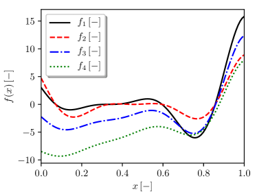
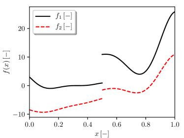
Figure 1: Forrester function (left) and discontinuous variant (right)

The function is defined in the domain $0\leq x\leq 1$ and the minimum is located $x^{*}=0.1426$ and given by $f(x^{*})=-0.9863$.

2.2 Rosenbrock function

The Rosenbrock function, also referred to as the Valley or Banana function, is a well-known D-dimensional optimization benchmark problem described by the following equation

$$f_{1}(\mathbf{x})=\sum_{i=1}^{D-1}100\left(x_{i+1}-x_{i}^{2}\right)^{2}+\left(1-x_{i}\right)^{2}$$ (9)

The global minimum is inside a long, narrow, parabolic shaped flat valley.

The function is unimodal, and the global minimum is located at $\mathbf{x}^{\star}=\{1,\dots,1\}^{\sf T}$ and equal to $f(\mathbf{x}^{\star})=0$. However, even though this valley is easy to find, convergence to the minimum is difficult. Note that there is also a local minimum at $\{-1,1,\dots,1\}^{\sf T}$ for $4\leq D\leq 7$. For the present problem the variable domain is defined as $-2\leq x_{i}\leq 2$ for $i=1,\dots D$.

The extension to multifidelity purposes is described by the following equations, where $f_{2}$ can be considered as a medium-fidelity level [9] and $f_{3}$ as the lowest fidelity [4].

$$f_{2}(\mathbf{x})=\sum_{i=1}^{D-1}50\left(x_{i+1}-x_{i}^{2}\right)^{2}+\left(-2-x_{i}\right)^{2}-\sum_{i=1}^{D}0.5x_{i}$$ (10)

$$f_{3}(\mathbf{x})=\dfrac{f_{1}(\mathbf{x})-4-\sum_{i=1}^{D}0.5x_{i}}{10+\sum_{i=1}^{D}0.25x_{1}}$$ (11)

The three-fidelity levels are shown for two dimensions in Figure 2.

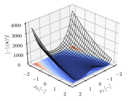
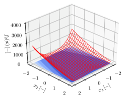
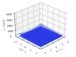
Figure 2: Rosenbrock Function: from left to right, $f_{1}$ (highest-fidelity), $f_{2}$ , and $f_{3}$ (lowest-fidelity)

2.3 Shifted-rotated Rastrigin function

To address real-world optimization problems, where the landscape of the objective function is usually multi-modal, the Rastrigin function is selected as benchmark. The function is shifted to change the position of the minimum and rotated to change the properties of the function itself within the variable space. The equation of the shifted-rotated Rastrigin function reads as follows

$$f_{1}(\mathbf{z})=\sum_{i=1}^{D}\left(z_{i}^{2}+1-\cos(10\pi z_{i})\right)$$ (12)

with

$$\mathbf{z}=R(\theta)(\mathbf{x}-\mathbf{x}^{\star})\,\,\,\,\,\mathrm{with}\,\,\,\,\,R(\theta)=\begin{bmatrix}\cos\theta&-\sin\theta\\ \sin\theta&\cos\theta\\ \end{bmatrix}$$ (13)

where $R$ is the rotation matrix in 2$D$ and can be extended to arbitrary dimension by using the Aguilera-Perez algorithm [1].

The variable ranges is defined such as $-0.1\leq x_{i}\leq 0.2$ for $i=1,\dots D$, rotation angle $\theta=0.2$, and optimum equal to $f(\mathbf{x}^{\star})=0$ at $\mathbf{x^{\star}}=\{0.1,\dots,0.1\}^{\sf T}$.

The fidelity levels can be defined following the work of Wang et al. [29], where a resolution error is defined as follows

$$e_{r}(\mathbf{z},\phi)=\sum_{i=1}^{D}a(\phi)\cos^{2}(w(\phi)z_{i}+b(\phi)+\pi)$$ (14)

with $a(\phi)=\Theta(\phi)$, $w(\phi)=10\pi\Theta(\phi)$, $b(\phi)=0.5\pi\Theta(\phi)$, and $\Theta(\phi)=1-0.0001\phi$. The fidelity levels are thus described as follows and depicted in Fig. 3.

$$f_{i}(\mathbf{z},\phi_{i})=f_{1}(\mathbf{z})+e_{r}(\mathbf{z},\phi_{i})~{}~{}~{}\mathrm{for}~{}~{}~{}\,i=1,2,3$$ (15)

with $\phi_{1}=10000$ (high-fidelity), $\phi_{2}=5000$ (medium-fidelity), and $\phi_{3}=2500$ (low-fidelity).

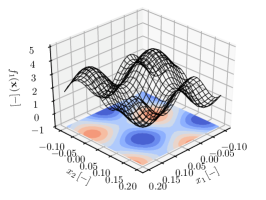
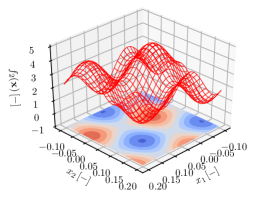
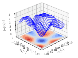
Figure 3: Shifted-rotated Rastrigin Function: from left to right, $f_{1}$ (highest-fidelity), $f_{2}$, and $f_{3}$ (lowest-fidelity)

2.4 Heterogeneous function

This problem employs heterogeneous non-polynomial analytic functions defined on unit hypercubes ($0\leq x_{i}\leq 1$ for $i=1,\dots D$) in one, two (taken from [7]), and three dimensions, with low-fidelity functions obtained by using linear additive and multiplicative bridge functions. The benchmark reads

$$\begin{cases}f_{1}(x)&=\sin[30(x-0.9)^{4}]\cos[2(x-0.9)]+(x-0.9)/2\\ f_{2}(x)&=(f_{1}(x)-1.0+x)/(1.0+0.25x)\end{cases}\qquad\mathrm{for}\qquad D=1$$ (16)

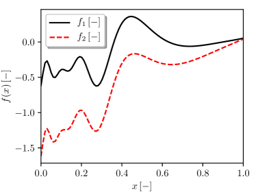
Figure 4: Heterogeneous function ($D=1$)

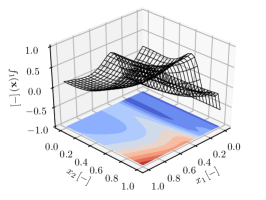
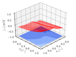
Figure 5: Heterogeneous function ($D=2$)

$$\begin{cases}f_{1}(\mathbf{x})&=\sin[21(x_{1}-0.9)^{4}]\cos[2(x_{1}-0.9)]+(x_{1}-0.7)/2+\sum_{i=2}^{D}ix_{i}^{i}\sin\left(\prod_{j=1}^{i}x_{j}\right)\\ f_{2}(\mathbf{x})&=(f_{1}(\mathbf{x})-2.0+\sum_{i=1}^{D}x_{i})/(5.0+\sum_{i=1}^{2}0.25ix_{i}-\sum_{i=3\atop D>2}^{D}0.25ix_{i})\end{cases}\,\,\,\mathrm{for}\,\,\,D\geq 2$$ (17)

The one- and two-dimensional functions are displayed together with their low-fidelity approximations in Figures 4 and 5. The optimum for $D=1$ is equal to $f(\mathbf{x}^{\star})=-0.625$ at $\mathbf{x^{\star}}=0.27550$, while for $D=2,3$ it is equal to $f(\mathbf{x}^{\star})=-0.5627123$ at $\mathbf{x^{\star}}=\{0,\dots,0\}^{\sf T}$.

2.5 Coupled Spring-Mass system

The proposed problem represents a general coupled spring-mass system. Consider two point masses $m_{1}$ and $m_{2}$ concentrated at their center of gravity and attached to each other by three springs, that operate according to Hooke’s law with constant $k_{1}$, $k_{2}$, and $k_{3}$. The mass of each spring is negligible and they restore after compression and extension. The masses can slide along a frictionless horizontal surface, while the first and last springs ($k_{1}$ and $k_{3}$) are attached to fixed walls, as shown in Figure 6.

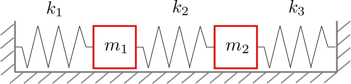
Figure 6: Coupled spring-masses system

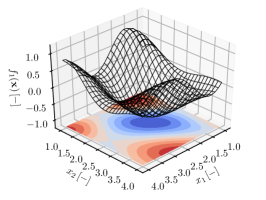
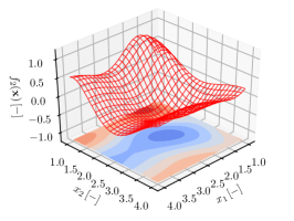
Figure 7: Spring-mass system ($D=2$, springs only)

Assume that $x_{1}(t)$ and $x_{2}(t)$ denote the mass positions along the horizontal surface, measured from their equilibrium positions, positive right and negative left. The equations of motion are given by the following system

$$\begin{cases}m_{1}\ddot{x}_{1}(t)&=-k_{1}x_{1}(t)+k_{2}[x_{2}(t)-x_{1}(t)]\\ m_{2}\ddot{x}_{2}(t)&=-k_{2}[x_{2}(t)-x_{1}(t)]-k_{3}x_{2}(t)\end{cases}$$ (18)

The equations are justified in the case of all positive variables by observing that the first two springs are elongated by $x_{1}$ and $x_{2}-x_{1}$, respectively. The last spring is compressed by $x_{2}$, which accounts for the minus sign. Eq. (18) can be written as a second-order vector-matrix system

$${\bf M}\ddot{{\bf x}}(t)={\bf Kx}(t)$$ (19)

where the displacement ${\bf x}$, mass matrix ${\bf M}$ and stiffness matrix $\bf K$ are defined by the following formulae

$${\bf x}=\left\{\begin{array}[]{c}x_{1}\\ x_{2}\end{array}\right\}\quad{\bf M}=\left[\begin{array}[]{cc}m_{1}&0\\ 0&m_{2}\end{array}\right]\quad{\bf K}=\left[\begin{array}[]{cc}-k_{1}-k_{2}&k_{2}\\ k_{2}&-k_{2}-k_{3}\end{array}\right]$$

This is a constant-coefficient homogeneous system of second-order ODEs the solution of which is given by

$${\bf x}(t)=\sum_{i=1}^{2}[a_{i}\cos(\omega_{i}t)+b_{i}\sin(\omega_{i}t)]{\bf z}_{i}$$ (20)

where $\omega_{i}=\sqrt{-\lambda_{i}}$ and $\lambda_{i}$ are the eigenvalues of the matrix ${\bf M}^{-1}{\bf K}$ and ${\bf z}_{i}$ are the corresponding eigenvectors. The constants $a_{i}$ and $b_{i}$ are determined by the initial conditions ${\bf x}(t=0)={\bf x}_{0}$ and $\dot{\bf x}(t=0)=\dot{\bf x}_{0}$

Converting Eq. 19 into a system of first-order ODEs and using the fourth-order accurate Runge-Kutta time-marching method yields a multifidelity analysis problem by varying the time-step size $\Delta t$. The proposed benchmark uses the initial conditions ${\bf x}_{0}=\{1\;0\}^{\sf T}$ and $\dot{\bf x}_{0}=\{0\;0\}^{\sf T}$ with two fidelity levels, defined by the time-step size, specifically equal to $\Delta t=0.01$ and 0.6. Two test are proposed, considering the position of the first mass $x_{1}$ at the time $t=6$ as the objective function: (MF5.1) springs $k_{1}$ and $k_{2}$ are the independent input variables with $1\leq(k_{1},k_{2})\leq 4$ and $k_{3}=k_{1}$, while the masses are constant ($m_{1}=m_{2}=1$), the optimum is equal to $f(\mathbf{x}^{\star})=-1$ at $\mathbf{x^{\star}}=\{2.467401,2.193245\}^{\sf T}$; (MF5.2) springs $k_{1}$ and $k_{2}$ and masses $m_{1}$ and $m_{2}$ are the independent input variables with $1\leq(k_{1},k_{2},m_{1},m_{2})\leq 4$ and $k_{3}=k_{1}$, the optimum is equal to $f(\mathbf{x}^{\star})=-1$ at $\mathbf{x^{\star}}=\{1.000000,3.946018,4.000000,3.286277\}^{\sf T}$. The two-dimensional (springs only) problem is shown in Fig. 7

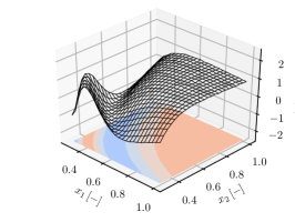
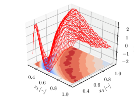
Figure 8: Paciorek function with noise: $f_{1}$ (left) and $f_{2}$ (right)

2.6 Paciorek Function

The Paciorek equation [28], which has localized and multi-modality properties, is considered and a normally distributed random noise parameter is added to the high- and low-fidelity equation to model the noise. The Paciorek function with noise term is defined as following

$$f_{1}(\mathbf{x})=\sin\left(\prod_{i=1}^{D}x_{i}\right)^{-1}+rand.normal(0,\alpha_{1})$$ (21)

$$f_{2}(\mathbf{x})=f_{1}(\mathbf{x})-9A^{2}\cos\left(\prod_{i=1}^{D}x_{i}\right)^{-1}+rand.normal(0,\alpha_{2})$$ (22)

$A$ is a parameter that models the error among the fidelities and can vary between 0 and 1, when $A=0$ the low- and high-fidelity equations are the same, while the change between the low-fidelity and high-fidelity models increases as the value of $A$ increases. In this study it is set as $A=0.5$, while $\alpha_{i}$ is the coefficient that defines the noise level. The benchmark is defined considering the variable ranges as $0.3\leq x_{i}\leq 1.0$ for $\forall i$. For the high-fidelity case a noise level is added to the equation which corresponds to approximately 5% of the response interval, as $\alpha_{1}=0.0125$. Accordingly, for the low-fidelity case much higher level of noise is added to the equation corresponding to 10% of the response interval, $\alpha_{2}=0.075$. The resulting response surfaces are shown in Fig. 8.

3 Setup of the Numerical Experiments

Table 3 summarizes the recommended set up for the assessment and comparison of the performance of multifidelity methods. The following subsections provide an overview of the rationale and the criteria motivating the recommendations along with additional complementary suggestions. The overview encompasses criteria for the assignment of the evaluation costs to the different fidelity levels as a fraction of the computational expense of the highest fidelity function, criteria for the initialization of the search, and criteria to terminate the search.

Table 2: Experiments setup summary

Function	Benchmark ID	$D$	Budget	Fidelity cost
				$f_{1}$	$f_{2}$	$f_{3}$	$f_{4}$
Forrester	MF1.1	1	100	1.00000E-0	5.00000E-1	1.00000E-1	5.00000E-2
Jump Forrester	MF1.2	1	100	1.00000E-0	2.00000E-1	-	-
	MF2.1	2	200	1.00000E-0	5.00000E-1	1.00000E-1	-
Rosenbrock	MF2.2	5	500	1.00000E-0	5.00000E-1	1.00000E-1	-
	MF2.3	10	1000	1.00000E-0	5.00000E-1	1.00000E-1	-
Shifted-rotated Rastrigin	MF3.1	2	200	1.00000E-0	6.25000E-2	3.90625E-3	-
	MF3.2	5	500	1.00000E-0	6.25000E-2	3.90625E-3	-
	MF3.3	10	1000	1.00000E-0	6.25000E-2	3.90625E-3	-
	MF4.1	1	100	1.00000E-0	2.00000E-1	-	-
Heterogeneous	MF4.2	2	200	1.00000E-0	2.00000E-1	-	-
	MF4.3	3	300	1.00000E-0	2.00000E-1	-	-
Springs	MF5.1	2	200	1.00000E-0	1.66667E-2	-	-
Springs-masses	MF5.2	4	400	1.00000E-0	1.66667E-2	-	-
Pacioreck	MF6	2	200	1.00000E-0	2.00000E-1	-	-

3.1 Fidelity cost assignment criteria

The $f_{1}({\bf x})$ functions are given the unitary cost $\lambda_{1}=1$, while their lower fidelity representations are assigned costs values as fractions of the $f_{1}({\bf x})$ cost. Table 3 proposes a set of cost assignments for the different fidelity representations of each of the benchmark problems. The values indicated for the shifted-rotated Rastrigin are determined according to the non-linear function proposed by Wang et al. [29] for the allocation of cost values to an arbitrary number of fidelities:

$$\lambda_{l}=\left(1/2^{l-1}\right)^{4}\qquad\forall\ l\geq 1$$ (23)

where higher values of the integer $l$ indicate representations of the objective functions at progressively lower levels or fidelity. Differently, the values indicated for the Forrester, the Rosenbrock, the Heterogeneous, and the Spring-Mass problems are driven by the shared experience within the AVT-331 research task group.

3.2 Initialization criteria

To assure a fair comparison across the different families of multifidelity methods, statistics over a set of different starting sample/points is recommended for all those methods that are not driven by an infill criterion. The cardinality and composition of the initial sample would not be constrained, but determined for or by the specific multifidelity method. This approach is preferred over the definition of specific initial samples to be used. The performance assessment would then consider statistics over the set of all the convergence histories.

3.3 Termination criteria

Real-world design problems are constrained by the limited time and computing resources available to conduct analysis, search, and optimization of the alternative candidate solutions. This motivates the choice to recommend conducting the experiments at given computational budgets assigned to the overall modelling and optimization task, rather than prescribing the maximum number of allowed iterations. The termination condition is reached when no computational budget is left. Table 3 indicates the computational budget assigned to each experiment in terms of equivalent number of evaluations of the high-fidelity representation.

4 Performance Assessment Metrics

Many different multifidelity approaches and original strategies have been developed, which may or may not rely on the use of a surrogate model combining the information from the different sources. The proposed metrics are selected to offer a comprehensive framework and to be able to compare a broad spectrum of different goal-driven multifidelity methods regardless of their specific features. Considering the initialization criteria recommended in Subsection 3.2, the performance of the different multifidelity methods will be assessed through statistics over the set of all the convergence histories.

Two types of metrics are defined: goal sensitive and goal insensitive. Goal-sensitive metrics evaluate the accuracy of the optima $\mathbf{x}^{\star}$ computed with MF approximations, whereas goal-insensitive metrics address the global accuracy of MF approximations over the design space. The ability to compute these metrics is very dependent on the nature of the design space, the benchmark complexity, and the methods employed for optimization. Construction and use of these metrics thus involves compromises, which are hopefully struck in a manner that hit a sweet spot of generality, usefulness, and feasibility.

With regards to goal-insensitive metrics, the global accuracy of MF approximations can be well interrogated for small $D$ and low benchmark complexity. As $D$ and benchmark complexity increase, the quantification of global accuracy rapidly becomes untenable through the effects of the curse of dimensionality (CoD) [2].

In contrast, global accuracy is not explicitly measured by goal-sensitive metrics, which simply assess computed optima. However, computing optima with global methods is also afflicted by the CoD, as is the global approximation of the functions that are optimized (whose cost can be mitigated by reduced sampling in unproductive areas).

Central to quantifying accuracy is a scaling of the design space. By scaling variables to equivalent ranges of variation (on the unit hypercube), the influence of parameter sensitivities can be balanced and the relative accuracy of computed optima better characterized. Unless stated otherwise, scaling of each design parameter is performed linearly between lower and upper limits supplied with the benchmark definition:

$$\tilde{x}_{k}\equiv{x_{k}-l_{k}\over u_{k}-l_{k}}\ \ \ (k=1,...,D),$$ (24)

or $\tilde{\mathbf{x}}=\mathbf{S}\left(\mathbf{x}-{\bf l}\right)$, where $\mathbf{S}$ is a diagonal scaling matrix and $\bf l$ is the lowest valued corner of the un-scaled design space. For notational convenience, the tilde notation is neglected unless needed for clarity. Lower and upper limits are provided for scaling and simplification, even when a parameter might potentially be unbounded. Scaling of the design space is independent of constraint surfaces existing in the benchmark problem.

Goal-insensitive metrics are defined first, which do not require knowledge of $\mathbf{x}^{\star}$. There are several competing goals for defining these metrics:

• High consistency, all methods should be evaluated in the same way;

• Low bias, the evaluation strategy should not be biased;

• High utility, the evaluation of metrics should be highly accurate and informative;

• Affordable cost, computing metrics should be affordable.

The goal-insensitive metric $\mathcal{E}_{\rm RMSE}$ records the root-mean-squared error between the highest fidelity model of the objective $f$, to an approximation to $f$, $\widehat{f}$, over the design space:

$$\mathcal{E}_{\rm RMSE}\equiv{1\over f_{\max}-f_{\min}}{\sqrt{\frac{1}{S}{\sum_{i=1}^{S}}(f(\mathbf{x}_{i})-\widehat{f}(\mathbf{x}_{i}))^{2}}},$$ (25)

where $i$ is the sample index, $S$ is the number of samples, and $f_{\min}$ and $f_{\max}$ are minimum and maximum values of $f$ observed over the training data:

$$f_{\min}\equiv\min_{\mathbf{x}_{i}}f(\mathbf{x}_{i}),\ \ \ f_{\max}\equiv\max_{\mathbf{x}_{i}}f(\mathbf{x}_{i}).$$ (26)

The sampling plan attempts to achieve two compromises: balancing computational cost with accuracy, and balancing consistency with low bias. The design spaces corresponding to the (inexpensive) analytical benchmarks are exhaustively sampled to rigorously assess method accuracy and performance for different functions. As benchmark complexity is increased, the amount of sampling can be reduced. Global accuracy cannot be computed for high-fidelity-based computational solutions, for their obvious high cost of sampling, but can be expected that MF-method strengths and weaknesses, in the context of global accuracy, can be extensively addressed with the analytical benchmarks proposed.

Goal-sensitive metrics are divided between metrics for the location of the optimum point (design accuracy) and metrics for the objective value (goal accuracy). The metrics are expressed as errors, which incorporate information about the optima assumed to be known apriori.

Three error metrics are defined for the benchmark problems, where optima are typically known analytically. These characterize normalized error in the design space, the objective function, and Euclidean distance in the normalized $\mathbf{x}$-$f$ hyperspace, respectively:

$$\mathcal{E}_{x}\equiv\dfrac{\|\hat{\mathbf{x}}^{\star}-\mathbf{x}^{\star}\|}{\sqrt{N}},$$ (27)

$$\mathcal{E}_{f}\equiv{f(\hat{\mathbf{x}}^{\star})-f_{\min}\over f_{\max}-f_{\min}},$$ (28)

$$\mathcal{E}_{t}\equiv\sqrt{\frac{\mathcal{E}_{x}^{2}+\mathcal{E}_{f}^{2}}{2}},$$ (29)

where $\mathbf{x}$ is the scaled array of design variables on the unit hypercube, $\hat{\mathbf{x}}^{\star}$ is the location of the optimum of the approximation to $f$ (in scaled parameters), and $f_{\min}$ and $f_{\max}$ are the minimum and maximum of $f$ in $\mathcal{A}$. The error metrics $\mathcal{E}_{x}$ and $\mathcal{E}_{f}$ evaluate design and goal accuracy, whereas the aggregated metric $\mathcal{E}_{t}$ introduced by Serani et. al. [25] evaluates accuracy in both senses, which can be of heightened significance when optima are in very flat or very peaky portions of the design space. Like the limits on design variables, $f_{\min}$ and $f_{\max}$ are provided with the benchmark to ensure consistent application by different MF methods. Reference values for the evaluation of the goal-sensitive metrics are summarized in Tab. 3. It should be emphasized that Eq. (28) utilizes an evaluation of the model of highest fidelity level at $\hat{\mathbf{x}}^{\star}$, a quantity computed with the MF approximation to $f$. Evaluation of the full-fidelity model is favored over that with the approximation to better characterize the true objective realized through the MF approximation.

Table 3: Summary of multifidelity benchmark values for the evaluation of the goal-sensitive metrics

Function	Benchmark ID	$D$	$\mathbf{x}^{\star}$	$f_{\min}$	$f_{\max}$
Forrester	MF1.1	1	7.5752E-1	-6.0207E-0	1.5830E+1
Jump Forrester	MF1.2	1	1.4260E-1	-9.8630E-1	2.5830E+1
	MF2.1	2	{1.0000, 1.0000}T	0.000E-0	3.6090E+3
Rosenbrock	MF2.2	5	{1.0000, …, 1.0000}T	0.000E-0	1.4436E+4
	MF2.3	10	{1.0000, …, 1.0000}T	0.000E-0	3.2481E+4
Shifted-rotated Rastrigin	MF3.1	2	{0.1000, 0.1000}T	0.000E-0	4.0200E-0
	MF3.2	5	{0.1000, …, 0.1000}T	0.000E-0	1.0050E+1
	MF3.3	10	{0.1000, …, 0.1000}T	0.000E-0	2.0100E+1
	MF4.1	1	2.7550E-1	-6.2500E-1	3.6151E-1
Heterogeneous	MF4.2	2	$\forall x_{1}=$ 0.000E-0	-5.6271E-1	1.8350E-0
	MF4.3	3	$\forall x_{1}=$ 0.000E-0	-5.6271E-1	4.3594E-0
Springs	MF5.1	2	{2.4674, 2.1932}T	-1.0000E-0	1.0000E-0
Springs-masses	MF5.2	4	{1.0000, 3.9460, 4.0000, 3.2863}T	-1.0000E-0	1.0000E-0
Pacioreck	MF6	2	$\forall x_{1}x_{2}=2/[(3+j)\pi]$ with $j=0,4$	-1.0000E-0	1.0000E-0

5 Concluding Remarks

A benchmark suite of analytical test function has been proposed to assess the efficiency and effectiveness of multifidelity optimization methods. The proposed benchmarks are meant to stress multifidelity optimization methods, dealing with various challenges typical of complex real-world optimization problems such as handling localized, multimodal, and discontinuous behaviors in the objective functions, as well as handling the possible presence of noise in the objective functions. The paper provides a set of standard problems, as well as recommended experimental setups and performance assessment metrics to support the rigorous test and comparison of different computational methods. Future work will include the performance assessment of a Gaussian process model and a trust region model to demonstrate the use cases.

References

- [1] A. Aguilera and R. Pérez-Aguila. General n-dimensional rotations. 2004.
- [2] R. Bellman. Dynamic programming. Press Princeton, New Jersey, 1957.
- [3] P. S. Beran, D. Bryson, A. S. Thelen, M. Diez, and A. Serani. Comparison of multi-fidelity approaches for military vehicle design. In AIAA AVIATION 2020 FORUM, page 3158, 2020.
- [4] D. E. Bryson and M. P. Rumpfkeil. Variable-fidelity surrogate modeling of lambda wing transonic aerodynamic performance. In AIAA SCITECH 2016 FORUM, 2016-0294.
- [5] D. E. Bryson and M. P. Rumpfkeil. Multifidelity quasi-newton method for design optimization. AIAA Journal, 56(10):4074–4086, 2018.
- [6] X. Cai, H. Qiu, L. Gao, L. Wei, and X. Shao. Adaptive radial-basis-function-based multifidelity metamodeling for expensive black-box problems. AIAA journal, 55(7):2424–2436, 2017.
- [7] D. L. Clark Jr, H.-R. Bae, K. Gobal, and R. Penmetsa. Engineering design exploration using locally optimized covariance kriging. AIAA Journal, 54(10):3160–3175, 2016.
- [8] C. Durantin, J. Rouxel, J.-A. Désidéri, and A. Glière. Multifidelity surrogate modeling based on radial basis functions. Structural and Multidisciplinary Optimization, 56(5):1061–1075, 2017.
- [9] S. Ficini, U. Iemma, R. Pellegrini, A. Serani, and M. Diez. An adaptive n-fidelity metamodel for design optimization via gaussian process regression. In AIAA AVIATION 2021 Forum, 2021.
- [10] A. I. Forrester, A. Sóbester, and A. J. Keane. Multi-fidelity optimization via surrogate modelling. Proceedings of the royal society A: mathematical, physical and engineering sciences, 463(2088):3251–3269, 2007.
- [11] M. Giselle Fernández-Godino, C. Park, N. H. Kim, and R. T. Haftka. Issues in deciding whether to use multifidelity surrogates. AIAA Journal, 57(5):2039–2054, 2019.
- [12] F. Grassi, G. Manganini, M. Garraffa, and L. Mainini. Resource aware multifidelity active learning for efficient optimization. In AIAA SciTech 2021 Forum, page 0894, 2021.
- [13] M. Guo, A. Manzoni, M. Amendt, P. Conti, and J. S. Hesthaven. Multi-fidelity regression using artificial neural networks: efficient approximation of parameter-dependent output quantities. Computer methods in applied mechanics and engineering, 389:114378, 2022.
- [14] E. Hoag and J. R. Doppa. Bayesian optimization meets search based optimization: A hybrid approach for multi-fidelity optimization. In Thirty-second AAAI conference on artificial intelligence, 2018.
- [15] S. Lee, F. Dietrich, G. E. Karniadakis, and I. G. Kevrekidis. Linking Gaussian process regression with data-driven manifold embeddings for nonlinear data fusion, 2019.
- [16] C. Li, P. Wang, and H. Dong. Kriging-based multi-fidelity optimization via information fusion with uncertainty. Journal of Mechanical Science and Technology, 32(1):245–259, 2018.
- [17] H. Li, Z. Huang, X. Liu, C. Zeng, and P. Zou. Multi-fidelity meta-optimization for nature inspired optimization algorithms. Applied Soft Computing, 96:106619, 2020.
- [18] B. Liu, S. Koziel, and Q. Zhang. A multi-fidelity surrogate-model-assisted evolutionary algorithm for computationally expensive optimization problems. Journal of computational science, 12:28–37, 2016.
- [19] J. Liu, H. Dong, and P. Wang. Multi-fidelity global optimization using a data-mining strategy for computationally intensive black-box problems. Knowledge-Based Systems, 227:107212, 2021.
- [20] H. B. Moss, D. S. Leslie, J. Gonzalez, and P. Rayson. GIBBON: General-purpose information-based bayesian optimisation. Journal of Machine Learning Research, 22(235):1–49, 2021.
- [21] C. Park, R. T. Haftka, and N. H. Kim. Remarks on multi-fidelity surrogates. Structural and Multidisciplinary Optimization, 55(3):1029–1050, 2017.
- [22] B. Peherstorfer, K. Willcox, and M. Gunzburger. Survey of multifidelity methods in uncertainty propagation, inference, and optimization. Siam Review, 60(3):550–591, 2018.
- [23] M. Raissi and G. E. Karniadakis. Deep multi-fidelity gaussian processes. CoRR, abs/1604.07484, 2016.
- [24] M. P. Rumpfkeil and P. S. Beran. Multi-fidelity, gradient-enhanced, and locally optimized sparse polynomial chaos and kriging surrogate models applied to benchmark problems. In AIAA SciTech 2020 Forum, 2020-0677.
- [25] A. Serani, C. Leotardi, U. Iemma, E. F. Campana, G. Fasano, and M. Diez. Parameter selection in synchronous and asynchronous deterministic particle swarm optimization for ship hydrodynamics problems. Applied Soft Computing, 49:313–334, 2016.
- [26] A. Serani, R. Pellegrini, J. Wackers, C.-E. Jeanson, P. Queutey, M. Visonneau, and M. Diez. Adaptive multi-fidelity sampling for CFD-based optimisation via radial basis function metamodels. International Journal of Computational Fluid Dynamics, 33(6-7):237–255, 2019.
- [27] J. Song, Y. Qiu, J. Xu, and F. Yang. Multi-fidelity sampling for efficient simulation-based decision making in manufacturing management. IISE Transactions, 51(7):792–805, 2019.
- [28] D. J. J. Toal. Some considerations regarding the use of multi-fidelity kriging in the construction of surrogate models. Structural and Multidisciplinary Optimization, 51(6):1223–1245, Dec. 2014.
- [29] H. Wang, Y. Jin, and J. Doherty. A generic test suite for evolutionary multifidelity optimization. IEEE Transactions on Evolutionary Computation, 22(6):836–850, 2017.
- [30] J. Yi, Y. Shen, and C. A. Shoemaker. A multi-fidelity RBF surrogate-based optimization framework for computationally expensive multi-modal problems with application to capacity planning of manufacturing systems. Structural and Multidisciplinary Optimization, 62(4):1787–1807, 2020.
- [31] X. Zhang, F. Xie, T. Ji, Z. Zhu, and Y. Zheng. Multi-fidelity deep neural network surrogate model for aerodynamic shape optimization. Computer Methods in Applied Mechanics and Engineering, 373:113485, 2021.