Beyond L1: Faster and Better Sparse Models with skglm

Abstract

We propose a new fast algorithm to estimate any sparse generalized linear model with convex or non-convex separable penalties. Our algorithm is able to solve problems with millions of samples and features in seconds, by relying on coordinate descent, working sets and Anderson acceleration. It handles previously unaddressed models, and is extensively shown to improve state-of-art algorithms. We release skglm, a flexible, scikit-learn compatible package, which easily handles customized datafits and penalties.

1 Introduction

Sparse generalized linear models play a central role in modern machine learning and signal processing. The Lasso (Tibshirani, 1996) and its derivatives (Zou and Hastie, 2005; Ng, 2004; Candes et al., 2008; Simon et al., 2013) have found numerous successful applications to large scale tasks in genomics (Ghosh and Chinnaiyan, 2005), vision (Mairal, 2010), or neurosciences (Strohmeier et al., 2016). This impact was made possible by two key factors: efficient algorithms and software implementations.

State-of-the-art algorithms for “smooth + non-smooth separable” problems predominantly rely on coordinate descent (CD, Tseng and S.Yun 2009; Nesterov 2012), which, when it can be applied, is more efficient than full gradient methods (Richtárik and Takáč, 2014, Sec. 6.1). Coordinate descent can even be improved with Nesterov-like acceleration, to obtain improved convergence rates (Lin et al., 2014; Fercoq and Richtárik, 2015). However, these better rates may fail to reflect in practical accelerations. On the contrary, Bertrand and Massias (2021) relied on Anderson acceleration (Anderson, 1965) to provide both better rates and practical acceleration for coordinate descent.

Even with efficient algorithms such as coordinate descent, the practical use of sparsity hits a computational barrier for problems with more than millions of features (Le Morvan and Vert, 2018). Multiple techniques have been proposed to make coordinate descent scale to huge problems. Notably, algorithms can be accelerated by reducing the number of variables to optimize over, using screening rules or working sets. Screening rules discard features from the problem in advance (El Ghaoui et al. 2010; Bonnefoy et al. 2015) or dynamically (Fercoq et al., 2015; Ndiaye et al., 2017). On the other side, working sets (Johnson and Guestrin, 2015; Massias et al., 2018) iteratively solve larger subproblems and progressively include variables identified as relevant.

For the Lasso and a few convex models, coordinate descent has been broadly disseminated to practitioners in off-the-shelf packages such as glmnet (Friedman et al., 2007) or scikit-learn (Pedregosa et al., 2011). More recently, celer, a state-of-the-art convex working set algorithm (Massias et al., 2020) allowed for successful applications of the Lasso in large scale problems in medicine (Reidenbach et al., 2021; Kim et al., 2021) or seismology (Muir and Zhan, 2021).

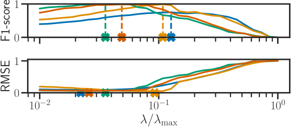
Figure 1: Regularization paths computed with our algorithm. Non-convex sparse penalties behave better than the L1 norm. Due to their lower bias, they achieve perfect support recovery, lower prediction error and their optimal regularization strength $\lambda$ in estimation (top) and prediction (bottom) correspond.

Yet the Lasso is limited: non-convex sparse models enjoy better theoretical and empirical properties (Breheny and Huang, 2011; Soubies et al., 2015). As illustrated in Figure 1, they yield sparser solutions than convex penalties and mitigate the intrinsic Lasso bias. Yet, they have not so often been applied to huge scale applications. This is mostly an algorithmic barrier: while coordinate descent can be applied to non-convex penalties (Breheny and Huang, 2011; Mazumder et al., 2011; Bolte et al., 2014), screening rules and working sets are heavily dependent on convexity or quadratic datafits (Rakotomamonjy et al., 2019, 2022).

In this work, we solve this issue by designing a state-of-the-art generic algorithm to solve a wide range of sparse generalized linear models. The contributions are the following:

• We propose a non-convex converging working set algorithm relying on Anderson accelerated coordinate descent. For a specific class of non-convex penalties, we show:

  1. Convergence of the proposed working set algorithm (Proposition 5).

  2. Support identification of coordinate descent (Proposition 10).

  3. Local convergence rates for the Anderson extrapolation (Proposition 13).

• We provide an extensive experimental comparison and we show state-of-the-art improvements on a wide range of convex and non-convex problems. In addition we release an efficient and modular python implementation, with a scikit-learn API, for practitioners to apply non-convex penalties to large scale problems.

2 Framework and proposed algorithm

2.1 Problem setting

In this paper, we consider problems of the form:

$$\hat{\beta}\in\operatorname*{argmin\,}_{\beta\in\mathbb{R}^{p}}\Phi(\beta)\triangleq\underbrace{F(X\beta)}_{\triangleq f(\beta)}+\sum_{j=1}^{p}g_{j}(\beta_{j})\enspace,$$ (0)

where $F$ is smooth, and the functions $g_{j}$ are proper and lower semicontinuous but not necessarily convex, whose proximal operator can be computed exactly. We write $g=\sum_{j}g_{j}$. Instances of (0) include convex estimators: the Lasso, the elastic net, the sparse logistic regression, the dual of SVM with hinge loss. They also include non-convex penalties: $\ell_{0.5}$ and $\ell_{2/3}$ penalties (Foucart and Lai, 2009), the minimax concave penalty (MCP, Zhang 2010) or SCAD (Zhang, 2010), both with regression and classification losses. Formally, the assumptions are the following.

Assumption 1.

$f:\mathbb{R}^{p}\to\mathbb{R}$ is convex and differentiable and for all $j\in[p]$, the restriction of $\nabla_{j}f$ to the $j$-th coordinate is $L_{j}$-Lipschitz: for all $(x,h)\in\mathbb{R}^{p}\times\mathbb{R}$, $|\nabla_{j}f(x+he_{j})-\nabla_{j}f(x)|\leq L_{j}\lvert{h}\rvert$.

Assumption 2.

For any $j\in[p],g_{j}:\mathbb{R}\to\mathbb{R}$ is proper, closed, and lower bounded.

Following Attouch and Bolte 2009; Bolte et al. 2014 we focus on finding a critical point of $\Phi$.

Definition 3.

Using the Fréchet subdifferential (Kruger, 2003), a critical point $x\in\mathbb{R}^{p}$ is a point which satisfies $-\nabla f(x)\in\partial g(x).$

Assumptions 1 and 2 are usual, and, under boundedness of the iterates, ensure convergence of forward-backward and coordinate descent algorithms to a critical point (Attouch et al. 2013, Thm 5.1, Bolte et al. 2014, Thm. 3.1). In addition, our work focuses on the case where $g_{j}$’s present non-differentiability points, leading to the following extended notion of sparsity.

Definition 4 (Generalized support).

The generalized support of $\beta\in\mathbb{R}^{p}$ is the set of indices $j\in[p]$ such that $g_{j}$ is differentiable at $\beta_{j}$: $\operatorname{gsupp}(\beta)=\{j\in[p]:\partial g_{j}(\beta_{j})\,\mathrm{is\;a\;singleton}\}.$

Penalties such as $\ell_{1}$, $\ell_{q}$ ($0<q<1)$, MCP or SCAD are only not differentiable at 0, and this corresponds to the usual notion of sparsity. But Definition 4 goes beyond sparsity and extends to estimators such as SVM, where $g_{j}=\iota_{[0,C]}$ and the generalized support is the complement of the support vectors’ set $\{j\in[p]:\beta_{j}=0\text{ or }\beta_{j}=C\}$. The generalized support of a critical point is usually of cardinality much smaller than $p$, and its knowledge makes the problem easier and faster to solve. Our working set algorithm exploits this structure in order to converge faster.

2.2 Proposed algorithm

The proposed algorithm exploits two main ideas:

• A working set strategy, able to handle a large class of convex and non-convex penalties (Algorithm 1).

• An Anderson accelerated coordinate descent for non-convex problems (Algorithm 2). The building blocks of Algorithm 2, coordinate descent (CD, Algorithm 3) and Anderson extrapolation (Anderson, Algorithm 4), can be found in Appendix A.

To avoid wasting computation on features outside the generalized support, working set algorithms iteratively select a subset of coordinates deemed important (the working set), and solve (0) restricted to them. The key question is thus the notion of important features. Stemming from Definition 3, we rank features by their violation of the optimality condition: $\mathrm{score}_{j}^{\partial}=\operatorname{dist}(-\nabla_{j}f(\beta),\partial g_{j}(\beta))\enspace.$ For example, the MCP Fréchet subdifferential at 0 is $\partial g_{j}(0)=[-\lambda,\lambda]$, and the proposed score reads

$$\mathrm{score}_{j}^{\partial}=\begin{cases}\max\{0,|\nabla_{j}f(\beta)|-\lambda\}\quad&\text{if}\quad\beta_{j}=0\enspace,\\ |\nabla_{j}f(\beta)+\nabla g_{j}(\beta_{j})|\quad&\text{otherwise}\enspace.\end{cases}$$ (1)

To control the working set growth, we use $\mathrm{score}_{j}^{\partial}$ to rank the features. Then, with $n_{k}=\max(n_{k-1},2\,|\operatorname{gsupp}(\beta^{(t)})|)$ we take the $n_{k}$ largest of them in the working set, while retaining features currently in the working set. This growth quickly rises to the unknown size of the generalized support while avoiding overshooting, as backed up by recent theory in Ndiaye and Takeuchi (2021).

Proposition 5.

Let $\mathcal{W}_{t}$ be the $t$-th working set. Suppose that Algorithm 2 converges toward a critical point, and for all $t\geq 0$, $\mathcal{W}_{t}\subset\mathcal{W}_{t+1}$, then the iterates of Algorithm 1 converge towards a critical point of (0).

input :  $X,\beta\in\mathbb{R}^{p},n_{\mathrm{out}}\in\mathbb{N},$

$n_{\mathrm{in}}\in\mathbb{N},\mathrm{ws\_size}\in\mathbb{N},\epsilon>0$

1 for $t=1,\ldots,n_{\mathrm{out}}$ do

2      

3      $\mathrm{score}=\big{(}\operatorname{dist}\left(-\nabla_{j}f(\beta),\partial g_{j}(\beta_{j})\right)\big{)}_{j\in[p]}$

4      $\mathrm{ws\_size}=\max(\mathrm{ws\_size},2\times|\operatorname{gsupp}(\beta)|)$

      // $\mathrm{ws\_size}$ features with largest scores

5      

6      $\mathrm{ws}=\mathrm{arg\_topK}(\mathrm{score},\mathrm{K=ws\_size})$

7      if $\max_{j\in[p]}\operatorname{dist}\left(-\nabla_{j}f(\beta),\partial g_{j}(\beta_{j})\right)\leq\epsilon$ then  stop ;

       else  // accelerated CD on working set

8      

9      $\beta\leftarrow\texttt{inner\_solver}(X,\beta,\mathrm{ws},n_{\mathrm{in}},\epsilon)$ ;

10      

return $\beta$

Algorithm 1 skglm (proposed)

input : $X,\beta^{(0)}\in\mathbb{R}^{p},\mathrm{ws}\subset[p],n_{\mathrm{in}}$, $\epsilon$, $M=5$

1

2for $k=1,\ldots,n_{\mathrm{in}}$ do

       $\beta^{(k)}\leftarrow\texttt{CD}(X,\beta^{(k-1)},X\beta,\mathrm{ws})$ ;

        // Algo. (3)

3      

4      if $k\,\mathrm{mod}\,M=0$ then

             // Algo. (4), $\mathcal{O}(M^{2}|\mathrm{ws}|+M^{3})$

5             $\beta_{\mathrm{ws}}^{\mathrm{extr}}\leftarrow\texttt{Anderson}(\beta_{\mathrm{ws}}^{(k-M)},\dots,\beta_{\mathrm{ws}}^{(M)})$

            // test objective $\mathcal{O}(n|\mathrm{ws}|)$

6             if  $\Phi(\beta_{\mathrm{ws}}^{\mathrm{extr}})<\Phi(\beta_{\mathrm{ws}}^{(k)})$  then

7                   $\beta_{\mathrm{ws}}^{(k)}\leftarrow\beta_{\mathrm{ws}}^{\mathrm{extr}};X\beta\leftarrow X_{\mathrm{ws}}\beta_{\mathrm{ws}}^{\mathrm{extr}}$

8      if  $\max_{j\in\mathrm{ws}}\operatorname{dist}\left(-\nabla_{j}f(\beta),\partial g_{j}(\beta_{j})\right)\leq\epsilon$  then  stop ;

9      

return $\beta^{(k)}$

Algorithm 2 inner_solver

Proof of Proposition 5 can be found in Section B.1. The second key ingredient to our algorithm is to use state-of-the-art Anderson accelerated coordinate descent for non-convex problems. In Section 2.3 we show that coordinate descent yields finite time support identification for a large class of non-convex problems (Proposition 10), which leads to acceleration (Proposition 13). As experiments demonstrate in Section 3, this rate allows our algorithm to surpass state-of-the-art solvers.

2.3 Anderson accelerated coordinate descent analysis for $\alpha$-semi-convex penalties

We now turn to our main technical contributions: we show that Algorithm 2 achieves finite time support identification (Proposition 10) of the generalized support (Definition 4) for specific class of non-smooth non-convex penalties (Assumption 6), which includes the MCP (Proposition 7). Based on Proposition 10, we are able to derive convergence rates for Anderson acceleration (Proposition 13).

We study our inner solver (Algorithm 2); for convenience we still refer to $\beta$ and $X$ for their counterparts restricted to the working set. The following assumptions are required.

Assumption 6 ($\alpha$-semi-convex).

For all $j\in[p]$ $g_{j}/L_{j}$ is $\alpha$-semi-convex, i.e., $g_{j}/L_{j}+\alpha\lVert{\cdot}\rVert^{2}/2$ is convex, with $\alpha<1$.

Note that in statistics, the admissible value range of hyperparameters for MCP and SCAD are datafit-dependent, (see Breheny and Huang 2011, Sec. 2.1, normalized columns and $\gamma>1=1/\left\lVert{X_{:j}}\right\rVert=1/L_{j}$ or Soubies et al. 2015, Eq. 4.2) and yields $\alpha$-semi-convexity for MCP and SCAD.

Proposition 7 ($\alpha$-semi-convexity of MCP).

Let $\operatorname{MCP}_{\lambda,\gamma}(x)\triangleq\begin{cases}\lambda\lvert{x}\rvert-\frac{x^{2}}{2\gamma}\enspace,&\text{if}\>\lvert{x}\rvert\leq\gamma\lambda\enspace,\\ \frac{1}{2}\gamma\lambda^{2}\enspace,&\text{if}\>\lvert{x}\rvert>\gamma\lambda\enspace.\end{cases}$
If $\gamma>1/L_{j}$, then $\operatorname{MCP}_{\lambda,\gamma}/L_{j}$ is $\alpha$-semi-convex with $\alpha=\tfrac{1}{2}(1+\frac{1}{\gamma L_{j}})$ (i.e., Assumption 6 holds).

Note that Assumption 6 does not hold for the $\ell_{q}$-penalties ($0<q<1$), for which we propose an alternative in Appendix C.

Assumption 8 (Existence).

(0) admits at least one critical point.

In Proposition 10, convergence of Algorithm 2 toward a critical point $\hat{\beta}$ is assumed, and the following assumption is made on this critical point.

Assumption 9 (Non degeneracy).

The considered critical point $\hat{\beta}\in\mathbb{R}^{p}$ is non-degenerated: for all $j\notin\operatorname{gsupp}(\hat{\beta})$,

$$-\nabla f_{j}(\hat{\beta})\in\,\mathrm{interior}(\partial g_{j}(\hat{\beta}_{j})).$$ (2)

Assumption 9 is a generalization of qualification constraints (Hare and Lewis, 2007, Sec. 1), and is usual in the machine learning literature (Zhao and Yu, 2006; Bach, 2008; Vaiter et al., 2015). For the $\ell_{1}$-norm, if the entries of the design matrix $X$ are drawn from an i.i.d normal distribution, then Assumption 9 holds with high probability (Candes and Tao, 2005; Rudelson and Vershynin, 2008).

Equipped with the previous assumptions we show that coordinate descent achieves model identification for this class of non-convex problems.

Proposition 10 (Model identification of CD).

Suppose

1. Assumptions 1, 2, 8 and 6 hold.

2. The sequence $(\beta^{(k)})_{k\geq 0}$ generated by coordinate descent (Algorithm 2 without extrapolation) converges toward a critical point $\hat{\beta}$.

3. Assumption 9 holds for $\hat{\beta}$.

Then, Algorithm 2 (without extrapolation) identifies the model in finitely many iterations: there exists $K>0$ such that for all $k\geq K$, $\beta_{\mathcal{S}^{c}}^{(k)}=\hat{\beta}_{\mathcal{S}^{c}}$.

In other words, for $k$ large enough, $\beta^{(k)}$ shares the generalized support of $\hat{\beta}$. The identification property was proved for a proximal gradient descent algorithm in the non-convex case (Liang et al., 2016) under the assumption that the non-smooth function $g$ is partly smooth (Lewis, 2002). For ourselves, Proposition 10 not rely on the partly smooth assumption to ensure identification property. Authors are not aware of previous identification results for coordinate descent in the non-convex case.

In addition, if $f$ and $g$ are locally regular on the generalized support at the considered critical point, our algorithm enjoys local acceleration when combined with Anderson extrapolation (Proposition 13).

Assumption 11 (Locally $\mathcal{C}^{3}$).

For all $j\in\mathcal{S}\triangleq\operatorname{gsupp}(\hat{\beta})$, $g_{j}$ is locally $\mathcal{C}^{3}$ around $\hat{\beta}_{j}$, and $f$ is locally $\mathcal{C}^{3}$ around $\hat{\beta}$.

Assumption 11 on the function $f$ is mild and holds for usual machine learning datafitting terms. Assumption 11 on the functions $g_{j}$, $j\in\mathcal{S}$, is stronger: for instance, for the MCP, it implies $\hat{\beta}_{j}\neq\gamma\lambda$ for all $j\in\mathcal{S}$. However this assumption is standard in the literature, see Liang et al. 2016, Sec. 3.3

Assumption 12.

(Local strong convexity) The Hessian of $f$ at the considered critical point $\hat{\beta}\in\mathbb{R}^{p}$, restricted to its generalized support $\mathcal{S}$, is positive definite, i.e., $\nabla^{2}_{\mathcal{S},\mathcal{S}}f(\hat{\beta})+\nabla^{2}_{\mathcal{S},\mathcal{S}}g(\hat{\beta})\succ 0$.

Assumption 12 requires local strong convexity restricted to the generalized support $\mathcal{S}$, which is standard in the MCP / SCAD literature (Breheny and Huang 2011, Section 4.1) and is usual to derive local linear rates of convergence (Liang et al., 2016, Section 3.3). For instance, for the Lasso, if the entries of the design matrix $X$ are drawn from a continuous distribution, then Assumption 12 holds with probability one (Tibshirani, 2013, Lemma 4).

Proposition 13.

Consider a critical point $\hat{\beta}$ and suppose

1. Assumptions 1, 2 and 8 hold.

2. The functions $f$ and $g_{j}$, $j\in[p]$ are piecewise quadratic (which is the case for the MCP regression).

3. The sequence $(\beta^{(k)})_{k\geq 0}$ generated by Anderson accelerated coordinate descent with updates from $1$ to $p$ and $p$ to $1$ (Algorithm 2 with extrapolation) converges to a critical point $\hat{\beta}$.

4. Assumptions 9, 11 and 12 hold for $\hat{\beta}$.

Then there exists $K\in\mathbb{N}$, and a $\mathcal{C}^{1}$ function $\psi:\mathbb{R}^{|\mathcal{S}|}\to\mathbb{R}^{|\mathcal{S}|}$ such that, for all $k\in\mathbb{N},k\geq K$:

$$\beta_{j}^{(k)} =\hat{\beta}_{j}\text{ , for all $j\in\mathcal{S}^{c}$, }$$ (3)

Let $T\triangleq\mathcal{J}\psi(\hat{\beta})$, $H\triangleq\nabla_{\mathcal{S},\mathcal{S}}^{2}f(\hat{\beta})+\nabla_{\mathcal{S},\mathcal{S}}^{2}g(\hat{\beta})$, $\zeta\triangleq(1-\sqrt{1-\rho(T)})/(1+\sqrt{1-\rho(T)})$ and $B\triangleq(T-\operatorname{Id})^{\top}(T-\operatorname{Id})$. Then $\rho(T)<1$ and the iterates of Anderson extrapolation enjoy local accelerated convergence rate:

$$\lVert{\beta_{\mathcal{S}}^{(k-K)}-\hat{\beta}_{\mathcal{S}}}\rVert_{B}\leq\Big{(}\sqrt{\kappa(H)}\tfrac{2\zeta^{M-1}}{1+\zeta^{2(M-1)}}\Big{)}^{(k-K)/M}\lVert{\beta_{\mathcal{S}}^{(K)}-\hat{\beta}_{\mathcal{S}}}\rVert_{B}\enspace.$$ (4)

The proof can be found in Section B.5.

Related work. Most Anderson acceleration convergence results are shown for quadratic objectives for specific algorithms: gradient descent (Golub and Varga, 1961; Anderson, 1965), ADMM (Poon and Liang, 2019), coordinate descent (Bertrand et al., 2020). Outside of the quadratic case, convergence results are usually significantly weaker (Scieur et al., 2016; Sidi, 2017; Brezinski et al., 2018; Mai and Johansson, 2019; Ouyang et al., 2020). Regarding the smooth non-convex case, Wei et al. (2021) proposed a stochastic Anderson acceleration and proved convergence towards a critical point. Proposition 13 generalizes Scieur et al. (2020, Prop 2.1) and Bertrand and Massias (2021, Prop. 4) to the proximal convex and $\alpha$-semi-convex cases. To our knowledge this is one of the first quantitative results for Anderson acceleration in a non-convex setting.

2.4 Comparison with existing work

Table 1: Most popular packages for sparse generalized linear models.

Name	Acceleration	Huge scale	Nncvx	Modular
glmnet (Friedman et al., 2010)	✗	✗	✗	✗  (Fortran)
scikit-learn (Pedregosa et al., 2011)	✗	✗	✗	✗  (Cython)
lightning (Blondel and Pedregosa, 2016)	✗	✗	✗	✓  (Cython)
celer (Massias et al., 2018)	✓	✓	✗	✗  (Cython)
picasso (Ge et al., 2019)	✗	✗	✓	✗   (C++)
pyGLMnet (Jas et al., 2020)	✗	✗✗	✗	✓  (Python)
fireworks (Rakotomamonjy et al., 2022)	✗	✓	✓	N.A.   (Python)
skglm (ours)	✓	✓	✓✓	✓   (Python)

In this section we compare our contribution to existing algorithms and implementations, which are summarized in Table 1. Huge scale refers to the fact that the algorithm can run on problems with millions of variables. Non-convex tells if the algorithm handles non-convex penalties. Modular indicates that it is easy to add a new model, through a different datafitting term or penalty.

The packages glmnet (Friedman et al., 2010), scikit-learn (Pedregosa et al., 2011) and lightning (Blondel and Pedregosa, 2016) implement coordinate descent (cyclic or random). They rely on compiled code such as Fortran or Cython, making it very difficult to implement new models or faster algorithms like working set. They do not handle non-convex penalties.

More recent algorithms such as blitz (Johnson and Guestrin, 2015), celer (Massias et al., 2018), picasso (Ge et al., 2019) or fireworks (Rakotomamonjy et al., 2022) use working set strategies. celer and blitz are state-of-the-art algorithms for the Lasso, but their score to prioritize features relies on duality. fireworks extends blitz to some non-convex penalties (writing as difference of convex functions), with $\mathrm{score}_{j}^{\mathrm{fireworks}}=\operatorname{dist}(-\nabla_{j}f(\beta),\partial g_{j}(0))$. Yet this rule does not consider the subdifferential of $g$ at the current point, but at 0, which is a coarse information. Finally, fireworks, building upon the seminal non convex working set solver of Boisbunon et al. (2014), does not provide accelerated convergence rates and does not come with a public implementation. picasso (Ge et al., 2019) lacks modularity (penalties are hardcoded), and the solver is not suited for huge scale (it does not support large sparse matrices). Deng and Lan (2019) proposed an algorithm based on inertially accelerated coordinate descent, which fails to provide practical speedups according to Bertrand and Massias (2021).

Contrary to these algorithms, ours is generic and relies only on the knowledge of $\nabla f$ and $\mathrm{prox}_{g}$. For any new penalty, this information can be written in a few lines of Python code, compiled with numba (Lam et al., 2015) for speed efficiency. We therefore improve state-of-the-art algorithms in the convex case, and generalize to virtually any datafit and penalty, even nonconvex.

3 Experiments

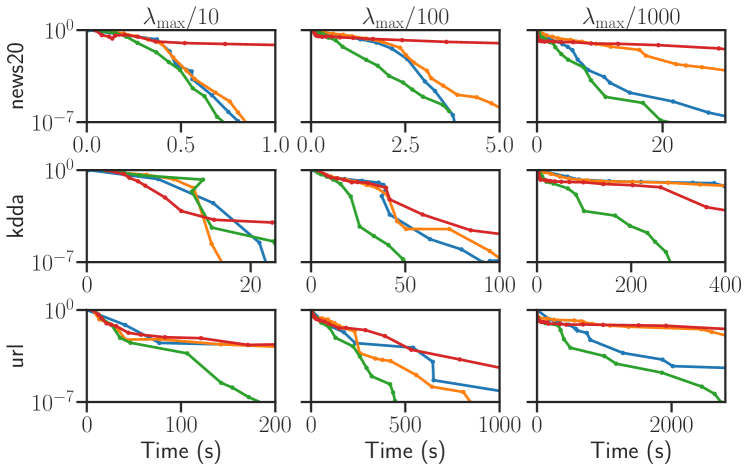
Figure 2: Lasso, duality gap. Normalized duality gap as a function of time for the Lasso on multiple datasets, for multiple values of $\lambda$.

Our package relying on numpy and numba (Lam et al., 2015; Harris et al., 2020) is attached in the supplementary material. An open source, fully tested and documented version of the code can be found at https://github.com/scikit-learn-contrib/skglm. We use datasets from libsvm (Fan et al. 2008, see table 2).

We compare multiple algorithms to solve popular Machine Learning and inverse problems: Lasso, Elastic net, multitask sparse regression, MCP regression. The compared algorithms are the following:

• scikit-learn (Pedregosa et al., 2011), which implements coordinate descent in Cython,

• celer (Massias et al., 2020), which combines working sets, screening rules, coordinate descent, and Anderson acceleration in the dual, in Cython,

• blitz (Johnson and Guestrin, 2015), which combines working sets with prox-Newton iterations (Lee et al., 2012) in C++,

• coordinate descent (CD, Tseng and S.Yun 2009),

• skglm (Algorithm 1, ours), using $M=5$ iterates for the Anderson extrapolation.

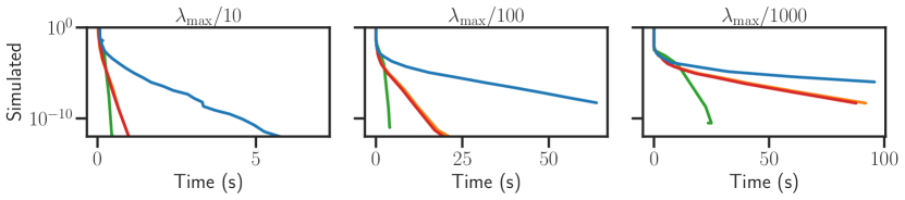
Figure 8: Elastic net, duality gap. Duality gap as a function of time for the elastic net on a synthetic dataset, for multiple values of $\lambda$.

Other solvers. Experiment per experiment, there exist niche solvers (such as aggressive Gap Safe Rules, Ndiaye et al. 2020). Since our goal is a general purpose algorithm able to deal with many models, we do not include them in the comparison. In addition, we focus on solving a single instance of (0), rather than a regularization path (i.e., a sequence of problems for multiple regularization strengths). As glmnet is designed to compute regularization paths, we could not include it in the comparison. The reader can refer to Johnson and Guestrin (2015, Fig. 4) or Figure 8 in Appendix E for comparisons on single optimization problems with glmnet; glmnet and additional algorithms are discussed in Appendix E.

How to do a fair comparison between solvers? To plot the convergence curves, we use the benchopt benchmarking package (Moreau et al., 2022). In order to automate and reproduce optimization benchmarks it treats solvers as black boxes. It launches them several times with increasing maximum number of iterations, and stores the resulting objective values and times to reach it. As each point on a solver curve is obtained in a different run, the curves are not monotonic, and there may be several points corresponding to the same time. This merely reflects the variability in solvers running time across runs; we refer to Figure 10 in Section E.6 for the inevitability of this phenomenon with black box solvers.

3.1 Convex problems

Lasso.

In Figure 2 we compare solvers for the Lasso: ($f=\frac{1}{2n}\left\lVert{y-X\cdot}\right\rVert^{2}$, $g_{j}=\lambda\lvert{\cdot}\rvert$). We parametrize $\lambda$ as a fraction of $\lambda_{\text{max}}=\lVert{X^{\top}y}\rVert_{\infty}/n$, smallest regularization strength for which $\hat{\beta}=0$. For large scale datasets (rcv1, news20), skglm yields performances better or similar to the state-of-the-art algorithms blitz and celer. For huge scale datasets (kdda and url), skglm yields significant speedups over them. The improvement over the popular scikit-learn can be of two orders of magnitude. Thus, while dealing with many more models, our algorithm still yields state-of-the-art speed for basic ones.

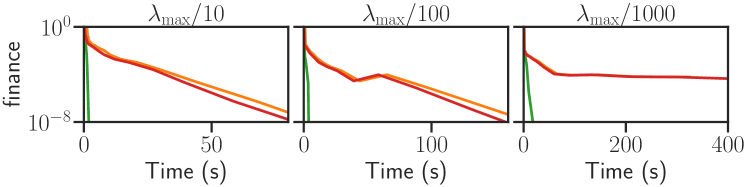
Figure 3: Elastic net, duality gap. Normalized duality gap as a function of time for the elastic net for multiple values of $\lambda$, $\rho=0.5$.

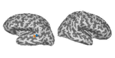
(a) $\ell_{2,1}$.

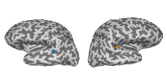
(b) $\ell_{2,0.5}$.

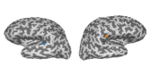
(c) Block MCP.

Figure 4: Real data, brain source locations recovered by convex and non-convex penalties after a right auditory stimulation. 4(a) shows that a convex penalty fails at identifying one source in each hemisphere, while 4(b) and 4(c) demonstrates the capability of non-convex penalties to recover the correct solution.

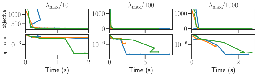
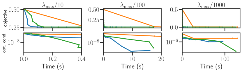
Figure 5: MCP, objective value and violation of first order condition. Objective value and violation of optimality condition of the iterates, $\mathrm{dist}(-\nabla f(\beta^{(k)}),\partial g(\beta^{(k)}))$, as a function of time for the MCP for multiple values of $\lambda$ ($\gamma=3$) on a simulated dense dataset (top) and the rcv1 dataset (normalized columns).

Elastic net.

Our approach easily generalizes to other problems, such as the elastic net ($f=\frac{1}{2n}\left\lVert{y-X\cdot}\right\rVert^{2}$, $g_{j}=\lambda(\rho\lvert{\cdot}\rvert+\frac{1-\rho}{2}(\cdot)^{2})$). Figure 3 shows the duality gap as a function of time for skglm (ours), sklearn, and our numba implementation of coordinate descent. The proposed algorithm is orders of magnitude faster than scikit-learn and vanilla coordinate descent, in particular for large datasets and low regularization parameter values (finance, $\lambda_{\max}/1000$). Note that blitz does not implement a solver for the elastic net. Many Lasso solvers would easily handle the elastic net, but relying on Cython/C++ code makes the implementation time-consuming. By contrast, it takes $40$ lines of code to define an $\ell_{1}+\ell_{2}$-squared penalty with our implementation. An additional experiment on the dual of SVM with hinge loss is in Section E.4.

3.2 Non-convex problems

In this subsection we propose a comparison on two non convex problems.

MCP regression.

MCP regression is (0) with $f=\frac{1}{2n}\left\lVert{y-X\cdot}\right\rVert^{2}$, $g_{j}=\operatorname{MCP}_{\lambda,\gamma}$ for $\gamma>1$. As usual for this problem, we scale the columns of $X$ to have norm $\sqrt{n}$. On Figure 5, we compare our algorithm to picasso on a dense dataset ($n=1000,p=5000$); as this package does not support large sparse design matrices, for the rcv1 dataset we use an iterative reweighted L1 algorithm (Candes et al., 2008). Since the derivative of the MCP vanishes for values bigger than $\lambda\gamma$, this approach requires solving weighted Lassos with some 0 weights. Up to our knowledge, our algorithm is the only efficient one with such a property. Our algorithm handles problems of large size, converges to a critical point, and, due to its progressive inclusion of features, is able to reach a sparser critical point than it competitors.

Application to neuroscience

To demonstrate the usefulness of our algorithm for practitioners, we apply it to the magneto-/electroencephalographic (M/EEG) inverse problem. It consists in reconstructing the spatial cortical current density at the origin of M/EEG measurements made at the surface of the scalp. Non-convex penalties (Strohmeier et al., 2015) exhibit several advantages over convex ones (Gramfort et al., 2013): they yield sparser physiologically-plausible solutions and mitigate the $\ell_{1}$ amplitude bias. Here the setting is multitask: $Y\in\mathbb{R}^{n\times T}$ and thus we use block penalties (details in Appendix D). We use real data from the mne software (Gramfort et al., 2014); the experiment is a right auditory stimulation, with two expected neural sources to recover in each auditory cortex. In Figure 4, while the $\ell_{2,1}$ penalty fails at localizing one source in each hemisphere, the non-convex penalties recover the correct locations. This emphasizes on the critical need for fast solvers for non-convex sparse penalties as well as our algorithm’s ability to handle the latter. In this work we focused on optimization-based estimators to solve the inverse problem, note that one could have resort to other techniques, such as Bayesian techniques (Ghosh and Doshi-Velez, 2017; Fang et al., 2020).

Ablation study. To evaluate the influence of the two components of Algorithm 1, an ablation study (Figure 6) is performed. Four algorithms are compared: with/without working sets and with/without Anderson acceleration. Figure 6 represents the duality gap of the Lasso as a function of time for multiple datasets and values of the regularization parameters $\lambda$ (parametrized as a fraction of $\lambda_{\text{max}}$). First, Figure 6 shows that working sets always bring significant speedups. Then, when combined with working set, Anderson acceleration bring significant speed-ups, especially for hard problems with low regularization parameters. An interesting observation is that on large scale datasets (news20 and finance) and for low regularization parameters ($\lambda_{\max}/100$ and $\lambda_{\max}/1000$) Anderson acceleration without working set does not bring acceleration. This highlights the importance of combining Anderson acceleration with working sets.

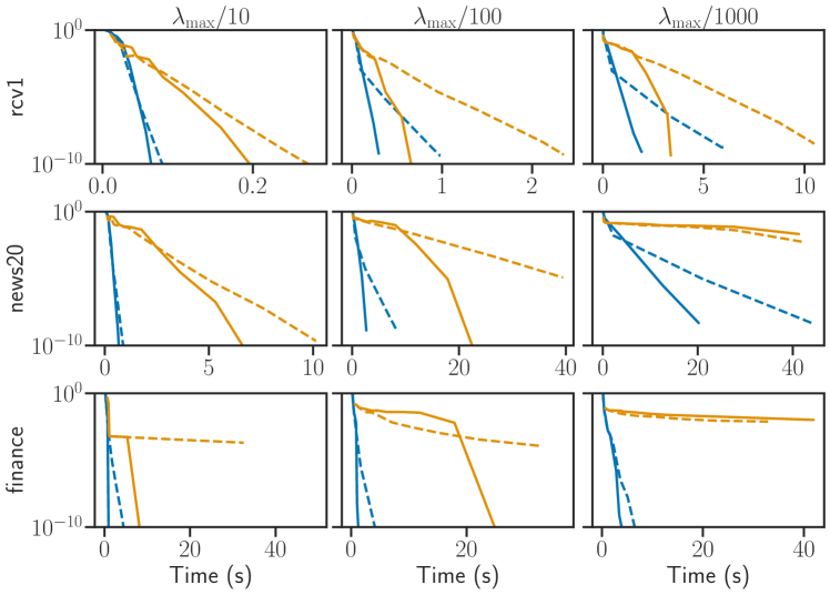
Figure 6: Lasso, duality gap. Normalized duality gap as a function of time for the Lasso.

Conclusion and broader impact.

In this paper, we have proposed an accelerated versatile algorithm for a specific class of non-smooth non-convex problems. Based on working sets, coordinate descent and Anderson acceleration, we have improved state of the art on convex problems, and handled previously out-of-reach problems. Thorough experiments demonstrated the speed and interest of our approach. A limitation of this work is the considered function class ($\alpha$-semi-convex), which can be seen as restrictive. One possible extension would be weakly convex functions (Davis and Drusvyatskiy, 2019, Sec. 1). We deeply believe that the high quality code provided will benefit to practitioners, and ease the use of non-convex penalties for real world problems, from neuroimaging to genomics. We proposed an optimization algorithm and do not see potential negative societal impacts.

Checklist

1. For all authors…

   1. Do the main claims made in the abstract and introduction accurately reflect the paper’s contributions and scope? [Yes]

   2. Did you describe the limitations of your work? [Yes] See limitations paragraph

   3. Did you discuss any potential negative societal impacts of your work? [Yes]

   4. Have you read the ethics review guidelines and ensured that your paper conforms to them? [Yes]

2. If you are including theoretical results…

   1. Did you state the full set of assumptions of all theoretical results? [Yes] See Propositions 10, 14 and 13.

   2. Did you include complete proofs of all theoretical results? [Yes] See Appendix B.

3. If you ran experiments…

   1. Did you include the code, data, and instructions needed to reproduce the main experimental results (either in the supplemental material or as a URL)? [Yes]

   2. Did you specify all the training details (e.g., data splits, hyperparameters, how they were chosen)? [Yes] See Section 3.

   3. Did you report error bars (e.g., with respect to the random seed after running experiments multiple times)? [N/A]

   4. Did you include the total amount of compute and the type of resources used (e.g., type of GPUs, internal cluster, or cloud provider)? [N/A]

4. If you are using existing assets (e.g., code, data, models) or curating/releasing new assets…

   1. If your work uses existing assets, did you cite the creators? [Yes] In particular we acknowledge the python ecosystem.

   2. Did you mention the license of the assets? [N/A]

   3. Did you include any new assets either in the supplemental material or as a URL? [Yes]

   4. Did you discuss whether and how consent was obtained from people whose data you’re using/curating? [N/A]

   5. Did you discuss whether the data you are using/curating contains personally identifiable information or offensive content? [N/A]

5. If you used crowdsourcing or conducted research with human subjects…

   1. Did you include the full text of instructions given to participants and screenshots, if applicable? [N/A]

   2. Did you describe any potential participant risks, with links to Institutional Review Board (IRB) approvals, if applicable? [N/A]

   3. Did you include the estimated hourly wage paid to participants and the total amount spent on participant compensation? [N/A]

Appendix A Algorithms

input :  $X\in\mathbb{R}^{n\times p},\beta\in\mathbb{R}^{p},X\beta\in\mathbb{R}^{n},L\in\mathbb{R}^{p},\mathrm{ws}\subset[p]$

1 for $j\in\mathrm{ws}$ do

       $\beta_{\mathrm{old}}\leftarrow\beta_{j}$ ;

        // $\mathcal{O}(1)$

2      

      $\beta_{j}\leftarrow\mathrm{prox}_{g_{j}/L_{j}}\left(\beta_{j}-\frac{1}{L_{j}}X_{:j}^{\top}\nabla F(X\beta)\right)$ ;

        // $\mathcal{O}(n)$

3      

      $X\beta\mathrel{+}=(\beta_{j}-\beta_{\mathrm{old}})X_{:j}$ ;

        // $\mathcal{O}(n)$

4      

return $\beta$

Algorithm 3 Coordinate descent epoch

init :  $\beta^{(0)},\dots,\beta^{(M)}\in\mathbb{R}^{|\mathrm{ws}|\times(M+1)}$

1

2$U=[\beta^{(1)}-\beta^{(0)},\ldots,\beta^{(M)}-\beta^{(M-1)}]\in\mathbb{R}^{|\mathrm{ws}|\times M}$

$c=(U^{\top}U)^{-1}\mathbf{1}_{M}\in\mathbb{R}^{M}$ ;

  // $\mathcal{O}(M^{2}|\mathrm{ws}|+M^{3})$

3

$c\mathrel{/}=\mathbf{1}_{M}^{\top}c$ ;

  // $\mathcal{O}(M)$

4

$\beta^{\mathrm{extr}}=\sum_{i=1}^{M}c_{i}\beta^{(i)}\in\mathbb{R}^{|\mathrm{ws}|}$ ;

  // $\mathcal{O}(M|\mathrm{ws}|)$

5

return $\beta^{\mathrm{extr}}$

Algorithm 4 Anderson extrapolation

Appendix B Proofs and propositions

B.1 Working set convergence (Proposition 5)

Proof.

Since $\mathcal{W}_{t}\subset\mathcal{W}_{t+1}$ after at most $p$ iterations, the working set is made of all the $p$ features. If Algorithm 1 stops when $|\mathcal{W}_{t}|<p$, then Bolte et al. (2014, Thm. 3.1) ensures that the inner solver converges towards a critical point of the restricted subproblem. Moreover, if the working set stops increasing, it means that for all $j\notin\mathcal{W}_{t}$, $\mathrm{score}_{j}^{\partial}$ is smaller than a given tolerance, hence satisfying the critical point condition of the global optimization problem.

If $|\mathcal{W}_{t}|=p$, the inner solver is used on the full optimization problem and Bolte et al. (2014, Thm. 3.1) ensures convergence towards a critical point of the latter.∎

B.2 $\alpha$-semi-convexity of MCP (Proposition 7)

Proof.

Let $j\in[p]$, $\gamma>\min_{j}1/L_{j}$ and $g_{j}\triangleq\operatorname{MCP}_{\lambda,\gamma}:x\mapsto\begin{cases}\lambda\lvert{x}\rvert-\frac{x^{2}}{2\gamma}\enspace,&\text{if}\>\lvert{x}\rvert\leq\gamma\lambda\\ \frac{1}{2}\gamma\lambda^{2}\enspace,&\text{if}\>\lvert{x}\rvert>\gamma\lambda\end{cases}$, $\alpha=\frac{1}{2}\left(1+\frac{1}{\gamma L_{j}}\right)$, and $h_{j}\triangleq\frac{g_{j}}{L_{j}}+\frac{\alpha}{2}\left\lVert{\cdot}\right\rVert^{2}$.

Since $\gamma>\min_{j}1/L_{j}$, $\alpha<1$. Moreover, for all $x>0$ such that, $\lvert{x}\rvert\leq\gamma\lambda$,

$$h_{j}(x) =\frac{\lambda\lvert{x}\rvert}{L_{j}}-\frac{x^{2}}{2\gamma L_{j}}+\frac{\alpha x^{2}}{2},\>\text{thus}$$ (5)

$$h_{j}^{\prime}(x) =\frac{\lambda}{L_{j}}+\frac{1}{2}\left(1-\frac{1}{\gamma L_{j}}\right)x,\>\text{thus}\enspace.$$ (6)

In addition, for all $x>0$ such that, $\lvert{x}\rvert>\gamma\lambda$

$$h_{j}(x) =\frac{1}{2}\gamma\lambda^{2}+\frac{\alpha x^{2}}{2},\>\text{thus}$$ (7)

$$h_{j}^{\prime}(x) =\frac{1}{2}\left(1+\frac{1}{\gamma L_{j}}\right)x\enspace.$$ (8)

Hence $h^{\prime}$ is an increasing function on $]0,+\infty[$, and thus $h$ is convex on $]0,+\infty[$. In addition, h is increasing, symmetric, and continuous, thus $h$ is convex on $\mathbb{R}$, and MCP is $\alpha$-semi-convex. ∎

B.3 Support identification for coordinate descent (Proposition 10)

For exposition purposes, the proof is first provided for proximal gradient descent.

Proof.

Proximal gradient descent. Here we generalize the results of Nutini (2018, Sec. 6.2.2) to semi-convex $g_{j}$’s. The updates of proximal gradient descent read:

$$\beta_{j}^{(k+1)}=\mathrm{prox}_{g_{j}/L}\left(\beta_{j}^{(k)}-\frac{1}{L}\nabla_{j}f(\beta^{(k)})\right)\enspace.$$ (9)

Let $\mathcal{S}$ be the generalized support of $\hat{\beta}$. Using Assumption 9, we have that for $j\notin\mathcal{S}$,

$$-\nabla_{j}f(\hat{\beta}) \in\mathrm{interior}(\partial g_{j}(\hat{\beta}_{j}))\enspace.$$ (10)

Combining Equation 10 with the Lipschitz continuity of the gradient (Assumption 1) and the convergence of $(\beta^{(k)})$ toward $\hat{\beta}$ yields that there exists $k\in\mathbb{N}$ such that

$$L(\beta_{j}^{(k)}-\hat{\beta}_{j})-\nabla_{j}f(\beta^{(k)})\in\partial g_{j}(\hat{\beta}_{j})\enspace.$$ (11)

Since $g_{j}/L$ is $\alpha$-semi-convex with $\alpha<1$, Equation 11 is equivalent to

$$\hat{\beta}_{j}=\mathrm{prox}_{g_{j}/L}\left(\beta_{j}^{(k)}-\frac{1}{L}\nabla_{j}f(\beta^{(k)})\right)\enspace.$$ (12)

By uniqueness of the proximity operator (direct consequence of Assumption 6), Equations 9 and 12 yield that there exists $K\in\mathbb{N}$ such that for all $k\geq K$, $\beta_{j}^{(k)}=\hat{\beta}_{j}$.

The proof for coordinate descent is similar and can be found in Section B.3. ∎

We prove the support identification for the coordinate descent algorithm Proposition 10.

Proof.

Proximal coordinate descent. Let us denote by $\beta^{(k,j)}$ the update at the epoch $k$ and changing the coordinate $j$ with the convention that $\beta^{(k,0)}=\beta^{(k)}$ and $\beta^{(k,p)}=\beta^{(k+1)}$. An update of proximal coordinate descent reads

$$\beta^{(k,j)}=\mathrm{prox}_{g_{j}/L_{j}}\left(\beta^{(k,j-1)}-\frac{1}{L_{j}}\nabla_{j}f(\beta^{(k,j-1)})\right)\enspace.$$ (13)

Let $\mathcal{S}$ be the generalized support of $\hat{\beta}$, a critical point of (0).

Using Assumption 9, we have that for $j\notin\mathcal{S}$,

$$-\nabla_{j}f(\hat{\beta}) \in\mathrm{interior}(\partial g_{j}(\hat{\beta}_{j}))\enspace.$$ (14)

Combining Equation 14 with the Lipschitz continuity of the gradient (Assumption 1) and the convergence of $(\beta^{(k)})$ toward $\hat{\beta}$ yields that there exists $k\in\mathbb{N}$ such that

$$L_{j}(\beta_{j}^{(k,j-1)}-\hat{\beta}_{j})-\nabla_{j}f(\beta^{(k,j-1)})\in\partial g_{j}(\hat{\beta}_{j})\enspace.$$ (15)

Since $g_{j}/L$ is $\alpha$-semi-convex with $\alpha<1$, Equation 15 is equivalent to

$$\hat{\beta}_{j}=\mathrm{prox}_{g_{j}/L_{j}}\left(\beta_{j}^{(k,j-1)}-\frac{1}{L_{j}}\nabla_{j}f(\beta^{(k,j-1)})\right)\enspace.$$ (16)

By uniqueness of the proximity operator (direct consequence of Assumption 6), Equations 13 and 16 yield that there exists $K\in\mathbb{N}$ such that for all $k\geq K$, $\beta_{j}^{(k)}=\hat{\beta}_{j}$. ∎

B.4 Local linear convergence (Proposition 14)

Here we extend in the proof of local linear convergence of coordinate descent from Klopfenstein et al. 2020 to the $\alpha$-semi-convex case. This property will be useful to show Proposition 13.

Proposition 14.

Consider a critical point $\hat{\beta}$ and suppose

1. Assumptions 1, 2, 8 and 6 hold.

2. The sequence $(\beta^{(k)})_{k\geq 0}$ generated by coordinate descent (Algorithm 2 without extrapolation) converges to a critical point $\hat{\beta}$.

3. Suppose Assumptions 9, 11 and 12 hold for $\hat{\beta}$.

Then there exists $K\in\mathbb{N}$, and a $\mathcal{C}^{1}$ function $\psi:\mathbb{R}^{|\mathcal{S}|}\to\mathbb{R}^{|\mathcal{S}|}$ such that, for all $k\in\mathbb{N},k\geq K$:

$$\beta_{j}^{(k)}=\hat{\beta}_{j}\text{ , for all $j\in\mathcal{S}^{c}$, }\text{ and }\,\beta_{\mathcal{S}}^{(k+1)}-\hat{\beta}_{\mathcal{S}}=\mathcal{J}\psi(\hat{\beta}_{\mathcal{S}})(\beta_{\mathcal{S}}^{(k)}-\hat{\beta}_{\mathcal{S}})+\mathcal{O}(\lVert{\beta_{\mathcal{S}}^{(k)}-\hat{\beta}_{\mathcal{S}}}\rVert^{2})\enspace,$$

and $\rho\left(\mathcal{J}\psi(\hat{\beta}_{\mathcal{S}})\right)<1\enspace,$ where $\mathcal{J}\psi$ is the Jacobian of $\psi$, and $\rho$ its spectral radius.

Note that under the hypothesis that $\Phi$ is $1/2$-Łojasiewicz, local linear convergence can be provided by Bolte et al. (2014, Remark 3.4).

Proof.

Let $\gamma_{j}=1/L_{j}$. Let $\mathcal{S}$ be the generalized support. Its elements are numbered as follows: $\mathcal{S}=\{j_{1},\ldots,j_{|\mathcal{S}|}\}$. We also define $\pi:\mathbb{R}^{|\mathcal{S}|}\to\mathbb{R}^{p}$ for all $\beta_{\mathcal{S}}\in\mathbb{R}^{|\mathcal{S}|}$ and all $j\in\mathcal{S}$ by

$$\pi(\beta_{\mathcal{S}})_{j}=\begin{cases}\beta_{j},&\text{if }j\in\mathcal{S}\\ \hat{\beta}_{j},&\text{if }j\in\mathcal{S}^{c}\enspace,\end{cases}$$

and for all $s\in[|\mathcal{S}|]$, $\mathcal{P}^{(s)}:\mathbb{R}^{|\mathcal{S}|}\to\mathbb{R}^{|\mathcal{S}|}$ is defined for all $u\in\mathbb{R}^{|\mathcal{S}|}$ and all $s^{\prime}\in[|S|]$ by

$$\left(\mathcal{P}^{(s)}(u)\right)_{s^{\prime}}=\begin{cases}u_{s^{\prime}}&\text{if }s\neq s^{\prime}\\ \mathrm{prox}_{\gamma_{j_{s}}g_{j_{s}}}\left(u_{s}-\gamma_{j_{s}}\nabla_{j_{s}}f(\pi(u))\right)&\text{if }s=s^{\prime}\enspace.\end{cases}$$

Once the model is identified (Proposition 10), we have that there exists $K\geq 0$ such that for all $k\geq K$

$$\beta^{(k)}_{\mathcal{S}^{c}} =\hat{\beta}_{\mathcal{S}^{c}}\quad\text{and}\quad$$

$$\beta^{(k+1)}_{\mathcal{S}}={\psi}(\beta^{(k)}_{\mathcal{S}}) \triangleq\mathcal{P}^{(|\mathcal{S}|)}\circ\ldots\circ\mathcal{P}^{(1)}(\beta^{(k)}_{\mathcal{S}})\enspace.$$ (17)

The proof of Proposition 14 follows three steps:

• First we show that the fixed-point operator ${\psi}$ is differentiable at $\hat{\beta}_{\mathcal{S}}$ (Lemma 15).

• Then we show that the Jacobian spectral radius of ${\psi}$ is strictly bounded by one (16 v)). Proof of 16 v) relies on 16 i), 16 ii), 16 iii) and 16 iv).

• Finally we conclude by a seconder order Taylor expansion of the fixed-point operator $\psi$.

Lemma 15 (Differentiability of the fixed-point operator).

The fixed-point operator ${\psi}$ is twice differentiable at $\hat{\beta}_{\mathcal{S}}$ with Jacobian:

$$\mathcal{J}{\psi}(\hat{\beta}_{\mathcal{S}}) =M^{-1/2}\underbrace{(\operatorname{Id}-B^{(|\mathcal{S}|)})\ldots(\operatorname{Id}-B^{(1)})}_{\triangleq A}M^{1/2}\enspace,$$ (18)

with

$$M \triangleq\nabla_{\mathcal{S},\mathcal{S}}^{2}f(\hat{\beta})+\nabla_{\mathcal{S},\mathcal{S}}^{2}g(\hat{\beta})\in\mathbb{R}^{|\mathcal{S}|\times|\mathcal{S}|}\enspace,\text{ and }$$ (19)

$$B^{(s)} \triangleq M_{:s}^{1/2}\frac{\gamma_{j_{s}}}{1+\gamma_{j_{s}}\nabla^{2}g_{j_{s}}(\hat{\beta}_{j_{s}})}M_{:s}^{1/2\top}\in\mathbb{R}^{|\mathcal{S}|\times|\mathcal{S}|}\enspace.$$ (20)

Lemma 15.

Let $j\in\mathcal{S}$, $\hat{\beta}_{j}=\mathrm{prox}_{\gamma_{j}g_{j}}(\hat{z}_{j})$, since $g_{j}$ is $\mathcal{C}^{1}$ at $\hat{\beta}_{j}$ (Assumption 11), we have $z_{j}=(\operatorname{Id}+\gamma_{j}g_{j}^{\prime})(\hat{\beta}_{j})\triangleq\phi(\hat{\beta}_{j})$, and $\hat{\beta}_{j}=\phi^{(-1)}(\hat{z}_{j})$ Since $j\in\mathcal{S}$, $g_{j}$ is of class $\mathcal{C}^{3}$ at $\hat{\beta}$ (Assumption 11), $\phi$ is $\mathcal{C}^{2}$ at $\hat{\beta}_{j}$. Moreover $\phi^{\prime}(\hat{\beta}_{j})=1+\gamma_{j}g_{j}(\hat{\beta}_{j})>0$ (using Assumption 6). Hence the inverse function theorem yields $\phi^{(-1)}$ is $\mathcal{C}^{1}$ at $\hat{z}_{j}\triangleq\phi(\hat{\beta}_{j})$, and

$$\mathrm{prox}^{\prime}(\hat{z}_{j}) =\phi^{(-1)^{\prime}}(\hat{z}_{j})$$ (21)

$$=\frac{1}{\phi^{\prime}(\phi^{(-1)}(\hat{z}_{j}))}$$ (22)

$$=\frac{1}{1+\gamma_{j}g_{j}^{\prime\prime}(\mathrm{prox}(\hat{z}_{j}))}$$ (23)

$$=\frac{1}{1+\gamma_{j}g_{j}^{\prime\prime}(\hat{\beta}_{j})}\enspace.$$ (24)

It follows that $\mathcal{P}^{(s)}$ is $\mathcal{C}^{2}$ at $\hat{\beta}_{\mathcal{S}}$. For all $s\in[|\mathcal{S}|]$, $\mathcal{P}^{(s)}$ is $\mathcal{C}^{2}$ at $\hat{\beta}_{\mathcal{S}}$. In addition, $\mathcal{P}^{(s)}(\hat{\beta}_{\mathcal{S}})=\hat{\beta}_{\mathcal{S}}$, thus $\psi\triangleq\mathcal{P}^{(|\mathcal{S}|)}\circ\ldots\circ\mathcal{P}^{(1)}$ is also $\mathcal{C}^{1}$ at $\hat{\beta}_{\mathcal{S}}$. To compute, the Jacobian of $\mathcal{P}^{(s)}$ at $\hat{\beta}_{\mathcal{S}}$, let us first notice that

$$\mathcal{J}\mathcal{P}^{(s)}(\hat{\beta}_{\mathcal{S}})^{\top}=\left(\begin{array}[]{c|c|c|c|c|c|c}e_{1}&\ldots&e_{s-1}&v_{s}&e_{s+1}&\ldots&e_{|\mathcal{S}|}\end{array}\right)\enspace,$$ (26)

where $v_{s}=\mathrm{prox}^{\prime}_{\gamma_{j_{s}}g_{j_{s}}}\left(\hat{z}_{j_{s}}\right)\left(e_{j_{s}}-\gamma_{j_{s}}\nabla^{2}_{j_{s},:}f(\hat{\beta})\right)$ and $\hat{z}_{j}=\hat{\beta}_{j}-\gamma_{j}\nabla_{j}f(\hat{\beta})$. This matrix can be rewritten

$$\mathcal{J}{\mathcal{P}^{(s)}}(\hat{\beta}_{\mathcal{S}}) =\operatorname{Id}_{|S|}-e_{s}e_{s}^{\top}+\mathrm{prox}^{\prime}_{\gamma_{j_{s}}g_{j_{s}}}\left(\hat{z}_{j_{s}}\right)\left(e_{s}e_{s}^{\top}-\gamma_{j_{s}}e_{s}e_{s}^{\top}\nabla^{2}f(\hat{\beta})\right)$$

$$=\operatorname{Id}_{|S|}-e_{s}e_{s}^{\top}\frac{\gamma_{j_{s}}}{1+\gamma_{j_{s}}g_{j}^{\prime\prime}(\hat{\beta}_{j_{s}})}\left(\nabla_{\mathcal{S},\mathcal{S}}g(\hat{\beta})+\nabla_{\mathcal{S},\mathcal{S}}^{2}f(\hat{\beta})\right)$$

$$=\operatorname{Id}_{|S|}-e_{s}e_{s}^{\top}\frac{\gamma_{j_{s}}}{1+\gamma_{j_{s}}g_{j}^{\prime\prime}(\hat{\beta}_{j_{s}})}M$$

$$=M^{-1/2}\left(\operatorname{Id}_{|S|}-M^{1/2}e_{s}e_{s}^{\top}\frac{\gamma_{j_{s}}}{1+\gamma_{j_{s}}g_{j}^{\prime\prime}(\hat{\beta}_{j_{s}})}M^{1/2}\right)M^{1/2}$$

$$=M^{-1/2}\left(\operatorname{Id}_{|S|}-B^{(s)}\right)M^{1/2}\enspace,$$

where

$$M\triangleq\nabla_{\mathcal{S},\mathcal{S}}^{2}f(\hat{\beta})+\nabla_{\mathcal{S},\mathcal{S}}^{2}g(\hat{\beta})\in\mathbb{R}^{|\mathcal{S}|\times|\mathcal{S}|}\enspace,$$ (27)

and

$$B^{(s)}\triangleq M^{1/2}_{:s}\frac{\gamma_{j_{s}}}{1+\gamma_{j_{s}}g_{j}^{\prime\prime}(\hat{\beta}_{j_{s}})}M_{:s}^{1/2\top}\in\mathbb{R}^{|\mathcal{S}|\times|\mathcal{S}|}.$$

The chain rule yields

$$\mathcal{J}{\psi}(\hat{\beta}_{\mathcal{S}}) =\mathcal{J}\mathcal{P}^{(|\mathcal{S}|)}(\hat{\beta}_{\mathcal{S}})\mathcal{J}\mathcal{P}^{(|\mathcal{S}|-1)}(\hat{\beta}_{\mathcal{S}})\ldots\mathcal{J}\mathcal{P}^{(1)}(\hat{\beta}_{\mathcal{S}})$$

$$=M^{-1/2}\underbrace{(\operatorname{Id}-B^{(|\mathcal{S}|)})(\operatorname{Id}-B^{(|\mathcal{S}|-1)})\ldots(\operatorname{Id}-B^{(1)})}_{\triangleq A}M^{1/2}\enspace.$$

∎

The following lemmas (16 i), 16 ii), 16 iii) and 16 iv)) aim at showing that the spectral radius of the Jacobian of the fixed-point operator $\psi$ is strictly bounded by one (16 v)).

Lemma 16.

1. The matrix $M$ defined in Equation 19 is symmetric definite positive.

2. For all $s\in[|\mathcal{S}|]$, the spectral radius of the matrix $B^{(s)}$ defined in Equation 20 is bounded by 1, i.e., $\lVert{B^{(s)}}\rVert_{2}\leq 1$.

3. For all $s\in[|\mathcal{S}|]$, $B^{(s)}/\lVert{B^{(s)}}\rVert$ is an orthogonal projector onto $\operatorname{Span}(M_{:s}^{1/2})$.

4. For all $s\in[|\mathcal{S}|]$ and for all $u\in\mathbb{R}^{S}$, if $\lVert{(\operatorname{Id}-B^{(s)})u}\rVert=\left\lVert{u}\right\rVert$ then $u\in\operatorname{Span}(M_{:s}^{1/2})^{\perp}$ and $(\operatorname{Id}-B^{(s)})u=u$.

5. The spectral radius of the Jacobian $\mathcal{J}{\psi}(\hat{\beta}_{\mathcal{S}})$ of the fixed-point operator $\psi$ is bounded by 1

   $$\rho(\mathcal{J}{\psi}(\hat{\beta}_{\mathcal{S}}))<1\enspace.$$ (28)

16 i).

Using Equation 19 yields

$$M =\nabla_{\mathcal{S},\mathcal{S}}^{2}f(\hat{\beta})+\nabla_{\mathcal{S},\mathcal{S}}^{2}g(\hat{\beta})\succ 0\quad\text{(using \lx@cref{creftypecap~refnum}{ass:local_str_cvx})}\enspace.$$ (29)

∎

16 ii).

$B^{(s)}$ is a rank one matrix which is the product of $\dfrac{\gamma_{j_{s}}}{1+\gamma_{j_{s}}\nabla^{2}{g_{j_{s}}}(\beta_{j_{s}})}M_{:s}^{1/2}$ and $M_{:s}^{1/2\top}$, its non-zeros eigenvalue is thus given by

$$\lVert{B^{(s)}}\rVert_{2} =\left|M^{1/2\top}_{:s}\dfrac{\gamma_{j_{s}}}{1+\gamma_{j_{s}}\nabla^{2}{g_{j_{s}}}(\beta_{j_{s}})}M_{:s}^{1/2}\right|$$

$$=\left|\dfrac{\gamma_{j_{s}}}{1+\gamma_{j_{s}}\nabla^{2}{g_{j_{s}}}(\beta_{j_{s}})}M_{s,s}\right|$$

$$=\left|\dfrac{\gamma_{j_{s}}}{1+\gamma_{j_{s}}\nabla^{2}{g_{j_{s}}}(\beta_{j_{s}})}\left(\nabla_{j_{s},j_{s}}^{2}f(\beta)+\nabla^{2}{g_{j_{s}}}(\beta_{j})\right)\right|\enspace.$$

$$=\dfrac{\overbrace{\gamma_{j_{s}}\nabla_{j_{s},j_{s}}^{2}f(\beta)}^{\leq 1}+\gamma_{j_{s}}\nabla^{2}{g_{j_{s}}}(\beta_{j_{s}})}{1+\gamma_{j_{s}}\nabla^{2}{g_{j_{s}}}(\beta_{j_{s}})}\leq 1\enspace.$$

∎

16 iv).

Let $s\in\mathcal{S}$,

$$\operatorname{Id}-B^{(s)} =\operatorname{Id}-\lVert{B^{(s)}}\rVert\frac{B^{(s)}}{\lVert{B^{(s)}}\rVert}=(1-\lVert{B^{(s)}}\rVert)\operatorname{Id}+\lVert{B^{(s)}}\rVert_{2}\operatorname{Id}-\lVert{B^{(s)}}\rVert_{2}\frac{B^{(s)}}{\lVert{B^{(s)}}\rVert_{2}}$$

$$=(1-\lVert{B^{(s)}}\rVert)\operatorname{Id}+\lVert{B^{(s)}}\rVert\underbrace{\left(\operatorname{Id}-\frac{B^{(s)}}{\lVert{B^{(s)}}\rVert_{2}}\right)}_{\text{projection onto }M_{:s}^{1/2\perp}}\enspace.$$ (30)

We will prove 16 iv) with a proof by absurd. Suppose that there exists $u\notin\operatorname{Span}(M_{:s}^{1/2})^{\perp}$ such that $\lVert{(\operatorname{Id}-B^{(s)})u}\rVert=\left\lVert{u}\right\rVert$.

There exists $\alpha\neq 0$, $u_{M_{:s}^{1/2\perp}}\in\operatorname{Span}(M_{:s}^{1/2})^{\perp}$ such that

$$u=\alpha M_{:s}^{1/2}+u_{M_{:s}^{1/2\perp}}\enspace.$$ (31)

Combining Equations 30 and 31 yields:

$$(\operatorname{Id}-B^{(s)})u =(1-\lVert{B^{(s)}}\rVert_{2})u+\lVert{B^{(s)}}\rVert_{2}u_{M_{:s}^{1/2\perp}}$$

$$\lVert{(\operatorname{Id}-B^{(s)})u}\rVert \leq\underbrace{|1-\lVert{B^{(s)}}\rVert_{2}|}_{=(1-\lVert{B^{(s)}}\rVert_{2})}\lVert{u}\rVert+\lVert{B^{(s)}}\rVert_{2}\underbrace{\lVert{u_{M_{:s}^{1/2\perp}}}\rVert}_{<\lVert{u}\rVert}<\lVert{u}\rVert\enspace,$$

which contradicts the supposition $\lVert{(\operatorname{Id}-B^{(s)})u}\rVert=\left\lVert{u}\right\rVert$. Thus $u\in\operatorname{Span}(M_{:s}^{1/2})^{\perp}$ and $(\operatorname{Id}-B^{(s)})u=u$. ∎

16 v).

. Let $u\in\mathbb{R}^{s}$ such that $\lVert{(\operatorname{Id}_{|\mathcal{S}|}-B^{(|\mathcal{S}|)})\dots(\operatorname{Id}_{|\mathcal{S}|}-B^{(1)})u}\rVert=\left\lVert{u}\right\rVert\enspace.$ Since

$$\lVert{(\operatorname{Id}_{|\mathcal{S}|}-B^{(|\mathcal{S}|)}\dots(\operatorname{Id}_{|\mathcal{S}|}-B^{(1)})}\rVert_{2}\leq\underbrace{\lVert{(\operatorname{Id}_{|\mathcal{S}|}-B^{(|\mathcal{S}|)})}\rVert_{2}}_{\leq 1}\times\dots\times\underbrace{\lVert{(\operatorname{Id}_{|\mathcal{S}|}-B^{(1)})}\rVert_{2}}_{\leq 1}\enspace,$$

we have for all $j\in\mathcal{S}$, $\lVert{(\operatorname{Id}_{|\mathcal{S}|}-B^{(s)})u}\rVert=\left\lVert{u}\right\rVert$. One can thus successively apply 16 iv) which yields $u\in\bigcap_{s\in[|\mathcal{S}|]}\operatorname{Span}{M_{:s}^{1/2}}^{\perp}\Leftrightarrow u\in\operatorname{Span}(M_{:1}^{1/2},\dots,M_{:|\mathcal{S}|}^{1/2})^{\perp}\enspace.$ Moreover $M^{1/2}$ has full rank, thus $u=0$ and $\lVert{(\operatorname{Id}_{|\mathcal{S}|}-B^{(|\mathcal{S}|)})\dots(\operatorname{Id}_{|\mathcal{S}|}-B^{(1)})}\rVert_{2}<1\enspace.$ From 16 v), $\lVert{A}\rVert_{2}<1$. Moreover $A$ and $\mathcal{J}{\psi}(\hat{\beta}_{\mathcal{S}})$ are similar matrices (Equation 18), then $\rho(\mathcal{J}{\psi}(\hat{\beta}_{\mathcal{S}}))=\rho(A)<1$. ∎

∎

B.5 Local acceleration (Proposition 13)

Proof.

Since Assumptions 1, 2, 8 and 9 hold, coordinate descent achieves finite time support identification (Proposition 10): there exists $l_{0}$ such that for all $l\geq l_{0}$, $\beta^{(l_{0}M+1)},\dots,\beta^{(l_{0}M+M)}$ shares the support of $\hat{\beta}$. Since Anderson acceleration linearly combines iterates from $\beta^{(l_{0}M+1)}$ to $\beta^{(l_{0}M+M)}$, it preserves the finite time identification property.

In addition, since Assumptions 9, 11 and 12 hold, and the functions $f$ and $g_{j}$, $j\in[p]$ are piecewise quadratic (by hypothesis), then Proposition 14 yields that there exists $K\in\mathbb{N}$ such that, for all $k\geq K$:

$$\beta_{\mathcal{S}^{c}}^{(k)} =\hat{\beta}_{\mathcal{S}^{c}}$$ (32)

$$\beta_{\mathcal{S}}^{(k+1)}-\hat{\beta}_{\mathcal{S}} =\mathcal{J}\psi(\hat{\beta}_{\mathcal{S}})(\beta_{\mathcal{S}}^{(k)}-\hat{\beta}_{\mathcal{S}})\enspace.$$ (33)

If the coordinate descent indices are picked from $1$ to $p$ and then form $p$ to $1$, then

$$T~\triangleq\mathcal{J}{\psi}(\hat{\beta}_{\mathcal{S}}) =M^{-1/2}(\operatorname{Id}-B^{(1)})\ldots(\operatorname{Id}-B^{(|\mathcal{S}|)})(\operatorname{Id}-B^{(|\mathcal{S}|)})\ldots(\operatorname{Id}-B^{(1)})M^{1/2}\enspace.$$ (34)

Based on Equation 34 one can apply Bertrand and Massias (2021, Prop. 4), which yields $\rho(T)<1$ and the iterates of Anderson extrapolation with parameter $M$ enjoy local accelerated convergence rate:

$$\lVert{\beta_{\mathcal{S}}^{(k-K)}-\hat{\beta}_{\mathcal{S}}}\rVert_{B}\leq\Big{(}\sqrt{\kappa(H)}\tfrac{2\zeta^{M-1}}{1+\zeta^{2(M-1)}}\Big{)}^{(k-K)/M}\lVert{\beta_{\mathcal{S}}^{(K)}-\hat{\beta}_{\mathcal{S}}}\rVert_{B}\enspace,$$ (35)

with $H\triangleq\nabla_{\mathcal{S},\mathcal{S}}^{2}f(\hat{\beta})+\nabla_{\mathcal{S},\mathcal{S}}^{2}g(\hat{\beta})$, $\zeta\triangleq(1-\sqrt{1-\rho(T)})/(1+\sqrt{1-\rho(T)})$, $B\triangleq(T-\operatorname{Id})^{\top}(T-\operatorname{Id})$. ∎

Appendix C Beyond $\alpha$-semi-convex penalties

C.1 Proposed score

When the $g_{j}$’s are not convex, the distance to the subdifferential can yield uninformative priority scores. This is in particular the case for $\ell_{q}$-penalties, with $0<q<1$.

Example 1.

The subdifferential of the $\ell_{0.5}$-norm at $0$ is: $\partial g(0)=\mathbb{R}$. Hence $0_{p}$ is a critical point for any $f$. For any $\beta$,

$$\operatorname{dist}(-\nabla_{j}f(\beta),\partial g_{j}(0))=0\enspace,$$ (36)

Thus if $\beta_{j}=0$, no matter the value of $\nabla_{j}f(\beta)$, feature $j$ is always assigned a score of 0, which is not relevant to discriminate important features.

A key observation to improve this rule is that, although $0_{p}$ is a critical point for any $f$, coordinate descent is able to escape it (Section C.2). Instead of considering critical point, we consider the more restrictive condition of being a fixed point of proximal coordinate descent:

$$\hat{\beta}_{j}=\mathrm{prox}_{g_{j}/L_{j}}\left(\hat{\beta}_{j}-\frac{1}{L_{j}}\nabla_{j}f(\hat{\beta})\right)\enspace.$$ (37)

We propose to rely on the violation of the fixed-point equation:

$$\mathrm{score}_{j}^{\mathrm{cd}}=|\beta_{j}-\mathrm{prox}_{g_{j}/L_{j}}(\hat{\beta}_{j}-\nabla_{j}f(\hat{\beta})/L_{j})|\enspace.$$ (38)

This is in a sense a restriction of the optimality conditions, since a fixed point is a critical point (while the converse may not be true).

Because this score only relies on $\nabla f$ and $\mathrm{prox}_{g_{j}}$, which are known for the overwhelming majority of instances of (0), our working set algorithm can address all of these, while being very simple to implement. This is in contrast with algorithm relying on duality, or on geometrical interpretations.

Remark 17.

Feature importance measures such as $\mathrm{score}_{j}^{\partial}$ and $\mathrm{score}_{j}^{\mathrm{cd}}$ have been considered in the convex case by Nutini et al. (2015, Sec. 8), while studying the Gauss-Southwell greedy coordinate descent selection rule. However, their approach is to compute the whole score vector (38), which requires a full gradient computation, in order to update a single coordinate: it is not a practical algorithm.

C.2 Coordinate descent escapes $0_{p}$

Let $f$ be a generic function satisfying Assumption 1. Suppose that coordinate descent is run on

$$\min f(\beta)+\lambda\sum_{1}^{p}\sqrt{\lvert{\beta_{j}}\rvert}\enspace,$$ (39)

initialized at $0_{p}$ (a critical point, as seen in Example 1). We show that if $\lambda$ is low enough, coordinate descent escapes this point. As coordinate descent is a descent method ($f$ is convex: the objective decreases strictly every time a coordinate’s value changes), it is sufficient to show that at least one coordinate is updated.

Let $j=\operatorname*{argmax\,}\lvert{\nabla_{j}f(0_{p})}\rvert$. When comes the time for coordinate $j$ to be updated, if some coordinate’s value has already changed, coordinate descent has escaped the origin. Otherwise, since the proximal operator of $x\mapsto\frac{\lambda}{L_{j}}\sqrt{x}$ is 0-valued exactly on $[-\frac{3}{2}\left(\frac{\lambda}{L_{j}}\right)^{2/3},\frac{3}{2}\left(\frac{\lambda}{L_{j}}\right)^{2/3}]$ (Wen et al., 2018, Table 1), if

$$\frac{1}{L_{j}}\lvert{\nabla_{j}f(0_{p})}\rvert>\frac{3}{2}\left(\frac{\lambda}{L_{j}}\right)^{2/3},\enspace$$ (40)

then the value of $\beta_{j}$ changes. Thus, for $\lambda<\left(\frac{2}{3}\frac{\lvert{\nabla_{j}f(0_{p})}\rvert}{L_{j}^{1/3}}\right)^{3/2}$, coordinate descent escapes the origin.

Appendix D Proximal operator of penalties in the multitask setting

In this section we consider a penalty on rows of matrices, i.e. letting $\phi$ be a 1 dimensional penalty, which is even, the whole penalty on $W\in\mathbb{R}^{p\times d}$ is

$$g(W)=\sum_{j=1}^{p}\phi(\lVert{W_{j:}}\rVert)$$ (41)

Since this penalty is separable, this brings us to solving:

$$\operatorname*{argmin\,}_{y\in\mathbb{R}^{d}}\frac{1}{2}\lVert{y-x}\rVert^{2}+\phi(\lVert{y}\rVert)\enspace.$$ (42)

Proposition 18.

The proximal operator of $y\mapsto\phi(\left\lVert{y}\right\rVert)$ is given by:

$$\mathrm{prox}_{\phi(\left\lVert{\cdot}\right\rVert)}(x)=\mathrm{prox}_{\phi}(\left\lVert{x}\right\rVert)\frac{x}{\left\lVert{x}\right\rVert}$$ (43)

Proof.

Notice that the minimum is necessarily attained at a point equal to $tx$, with $t\geq 0$: indeed, for any $y$, $\frac{\left\lVert{y}\right\rVert}{\left\lVert{x}\right\rVert}x$ yields $\phi(\left\lVert{\frac{\left\lVert{y}\right\rVert}{\left\lVert{x}\right\rVert}x}\right\rVert)=\phi(\left\lVert{y}\right\rVert)$, and since:

$$\left\lVert{\frac{\left\lVert{y}\right\rVert}{\left\lVert{x}\right\rVert}x-x}\right\rVert^{2}=\left\lVert{y}\right\rVert^{2}-2\left\lVert{y}\right\rVert\left\lVert{x}\right\rVert+\left\lVert{x}\right\rVert^{2}\leq\left\lVert{y}\right\rVert^{2}-2\langle y,x\rangle+\left\lVert{x}\right\rVert^{2}=\left\lVert{y-x}\right\rVert^{2}\enspace,$$ (44)

it achieves lower objective value in (42) than $y$. Hence the problem transforms into a 1 dimensional one:

$$\operatorname*{argmin\,}_{y\in\mathbb{R}^{d}}\frac{1}{2}\left\lVert{y-x}\right\rVert^{2}+\phi(\left\lVert{y}\right\rVert) =\left(\operatorname*{argmin\,}_{t\geq 0}\frac{1}{2}(t-1)^{2}\left\lVert{x}\right\rVert^{2}+\phi(\lvert{t}\rvert\left\lVert{x}\right\rVert))\right)x$$

$$=\left(\operatorname*{argmin\,}_{t\in\mathbb{R}}\frac{1}{2}(t-1)^{2}\left\lVert{x}\right\rVert^{2}+\phi(t\left\lVert{x}\right\rVert))\right)x\quad\quad\quad\text{($\phi$ is even)}$$

$$=\left(\operatorname*{argmin\,}_{t\in\mathbb{R}}\frac{1}{2}(t-\left\lVert{x}\right\rVert)^{2}+\phi(t))\right)\frac{x}{\left\lVert{x}\right\rVert}$$

$$=\mathrm{prox}_{\phi}(\left\lVert{x}\right\rVert)\frac{x}{\left\lVert{x}\right\rVert}\enspace.$$ (45)

∎

Appendix E Supplementary experiments

E.1 Datasets characteristics

Table 2: Datasets characteristics.

Datasets	#samples $n$	#features $p$	density
rcv1	$20\,242$	$19\,959$	$3.6\text{\times}{10}^{-3}$
news20	$19\,996$	$1\,355\,191$	$3.4\text{\times}{10}^{-4}$
finance	$16\,087$	$4\,272\,227$	$1.4\text{\times}{10}^{-3}$
kdda	$8\,407\,752$	$20\,216\,830$	$1.8\text{\times}{10}^{-6}$
url	$2\,396\,130$	$3\,231\,961$	$3.6\text{\times}{10}^{-5}$

E.2 ADMM comparison

ADMM can solve a larger range of optimization problems than CD (Boyd et al., 2011, Eq. 3.1). Yet, for the Lasso, ADMM requires solving a $p\times p$ linear system at each primal iteration. This is too costly: ADMM is usually not included in Lasso benchmarks (e.g. Johnson and Guestrin 2015). Our algorithm outperforms the implementation of Poon and Liang (2019) as visible on Figure 7.

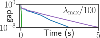
Figure 7: ADMM, duality gap. Duality gap as a function of time for the elastic net on a synthetic dataset.

E.3 glmnet comparison

glmnet uses a combination of coordinate descent and strong rules to solve the Lasso, elastic net and other L1 + L2 regularized convex problems. By design of the strong rules (Tibshirani et al., 2012), glmnet is only usable when a sequence of problems must be solved, with decreasing regularization strength $\lambda$: the so-called homotopy/continuation path setting. In addition, even prompted to solve a given path, the implementation of glmnet does no go up to the smallest $\lambda$ if some statistical criterion stops improving from one $\lambda$ to the other. Thus, in practice it is nearly impossible to get glmnet to solve a single instance of (0) for a given value of $\lambda$.

E.4 Benchmark on SVM

Our proposed algorithm can be used with various datafits and penalties. The SVM primal optimization problem reads

$$\operatorname*{argmin\,}_{\beta\in\mathbb{R}^{p}}\frac{1}{2}\lVert{\beta}\rVert^{2}+C\sum_{i=1}^{n}\max(0,1-y_{i}X_{i:}^{\top}\beta)\enspace.$$ (46)

The dual of Equation 46 falls in the framework encompassed by our algorithm, it writes:

$$\operatorname*{argmin\,}_{\alpha\in\mathbb{R}^{n}} \frac{1}{2}\alpha^{\top}Q\alpha-\sum_{i=1}^{n}\alpha_{i}$$ (47)

$$\text{s.t.}0\leq\alpha_{i}\leq C\enspace,$$

where $Q_{ij}=y_{i}y_{j}X_{i:}^{\top}X_{j:}$. The datafit is then a quadratic function which we seek to minimize subject to the constraints that $\alpha_{i}\in[0,C]$. Equation 47 is equivalent to the minimization of the following problem:

$$\operatorname*{argmin\,}_{\alpha\in\mathbb{R}^{n}}\alpha^{\top}Q\alpha-\sum_{i=1}^{n}\alpha_{i}+\iota_{[0,C]}(\alpha_{i}),$$ (47)

where $\iota_{[0,C]}$ is the indicator function of the set $[0,C]$. We also have that the equation link between Equation 46 and (47) is given by

$$\beta=\sum_{i=1}^{n}y_{i}\alpha_{i}X_{i:}\enspace.$$ (48)

We solved (47) on the real dataset real-sim. We compared our algorithm with a coordinate descent approach (CD), the scikit-learn solver based on liblinear, the l-BFGS (Liu and Nocedal, 1989) algorithm, lightning, and the proposed algorithm (skglm). Figure 9 shows the suboptimality objective value as a function of the time for the different solvers. The optimization problem was solved for three different regularization values controlled by the parameter $C$ which was set to $0.1$, $1.0$ and $10.0$. As Figure 9 illustrates our algorithm is faster than its counter parts. The difference is larger as the optimization problem is more difficult to solve i.e., when $C$ gets large.

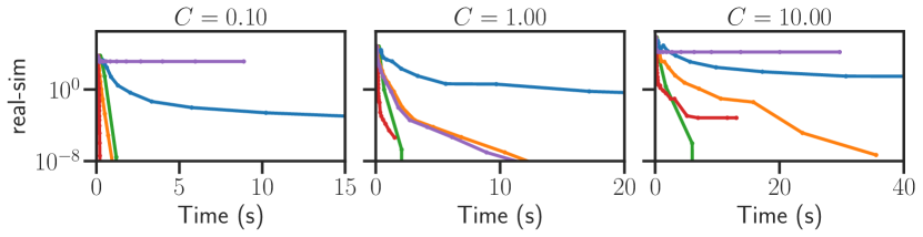
Figure 9: SVM, Suboptimality. Suboptimality as a function of time for the dual SVM optimization (47).

E.5 Sparse recovery with non-convex penalties

In Figure 1, to demonstrate the versatility of our approach, we provide a short benchmark of sparse regression, using convex and non-convex penalties. The data is simulated, with $n=1000$ samples and $p=2000$ features with correlation between features $j$ and $j^{\prime}$ equal to $0.6^{\lvert{j-j^{\prime}}\rvert}$. The true regression vector $\beta^{*}$ has $200$ non zero entries, equal to 1. The observations are equal to $y=X\beta^{*}+\varepsilon$ where $\varepsilon$ is centered Gaussian noise with variance such that $\lVert{X\beta^{*}}\rVert/\lVert{\varepsilon}\rVert=5$. On Figure 1 we show the regularization path (value of solution found for ever $\lambda$ computed with our algorithm). Note that despite convergence being only guaranteed towards a local minima, the performance of non-convex estimators is still far better than the global minimizer of the Lasso. We see that the non-convex penalties are better at recovering the support. The time to compute the regularization paths is similar for the 4 models, around 1 s. Thanks to our flexible library, we intend to bring these improvements to practitioners at a large scale.

E.6 Variations in the convergence curves

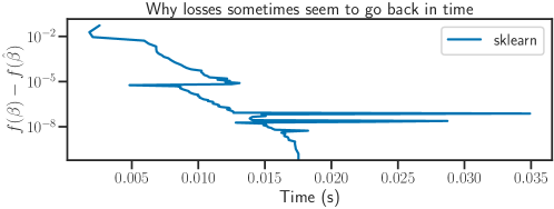
Figure 10: Typical curve aspect caused by variations in solver running time from one run to another (scikit-learn, Lasso problem).

By design of the benchopt library that we used for reproducible experiments, solvers are treated as black boxes, for which one only controls the number of iteration performed. It is thus not possible to monitor the time and losses in a single run of a given solver. Instead, the solver is run for 1 iteration, then 2 (starting again from 0), then 3, etc. This allows to obtain a convergence curve for a solver without interfering with its inner mechanisms. One drawback is that, because of variability in code execution time, it may happen that the run with $K+1$ iterations takes less time than the run with $K$ iterations, for example in Figure 10 – although it performs more iterations and thus usually decreases the objective more. Then, the curves seem to go back in time. The variability can be damped by running the experiment several times and averaging the results, which we did when the total running time allowed it. Otherwise, these variations should indicate that, as all measurements, convergence curves as a function of time are noisy.

References

- Anderson (1965) D. G. Anderson. Iterative procedures for nonlinear integral equations. Journal of the ACM, 12(4):547–560, 1965.
- Attouch and Bolte (2009) H. Attouch and J. Bolte. On the convergence of the proximal algorithm for nonsmooth functions involving analytic features. Mathematical Programming, 116(1):5–16, 2009.
- Attouch et al. (2013) H. Attouch, J. Bolte, and B. F. Svaiter. Convergence of descent methods for semi-algebraic and tame problems: proximal algorithms, forward–backward splitting, and regularized Gauss–Seidel methods. Mathematical Programming, 137(1):91–129, 2013.
- Bach (2008) F. Bach. Consistency of the group Lasso and multiple kernel learning. J. Mach. Learn. Res., 9:1179–1225, 2008.
- Bertrand and Massias (2021) Q. Bertrand and M. Massias. Anderson acceleration of coordinate descent. In AISTATS, 2021.
- Bertrand et al. (2020) Q. Bertrand, Q. Klopfenstein, M. Blondel, S. Vaiter, A. Gramfort, and J. Salmon. Implicit differentiation of lasso-type models for hyperparameter optimization. ICML, 2020.
- Blondel and Pedregosa (2016) M. Blondel and F. Pedregosa. Lightning: large-scale linear classification, regression and ranking in python, 2016.
- Boisbunon et al. (2014) A. Boisbunon, R. Flamary, and A. Rakotomamonjy. Active set strategy for high-dimensional non-convex sparse optimization problems. In 2014 IEEE International Conference on Acoustics, Speech and Signal Processing (ICASSP), pages 1517–1521. IEEE, 2014.
- Bolte et al. (2014) J. Bolte, S. Sabach, and M. Teboulle. Proximal alternating linearized minimization for nonconvex and nonsmooth problems. Mathematical Programming, 146(1):459–494, 2014.
- Bonnefoy et al. (2015) A. Bonnefoy, V. Emiya, L. Ralaivola, and R. Gribonval. Dynamic screening: accelerating first-order algorithms for the Lasso and Group-Lasso. IEEE Trans. Signal Process., 63(19):20, 2015.
- Boyd et al. (2011) S. Boyd, N. Parikh, and E. Chu. Distributed optimization and statistical learning via the alternating direction method of multipliers. Now Publishers Inc, 2011.
- Breheny and Huang (2011) P. Breheny and J. Huang. Coordinate descent algorithms for nonconvex penalized regression, with applications to biological feature selection. The annals of applied statistics, 5(1):232, 2011.
- Brezinski et al. (2018) C. Brezinski, M. Redivo-Zaglia, and Y. Saad. Shanks sequence transformations and anderson acceleration. SIAM Review, 60(3):646–669, 2018.
- Candes and Tao (2005) E. J. Candes and T. Tao. Decoding by linear programming. IEEE transactions on information theory, 51(12):4203–4215, 2005.
- Candes et al. (2008) E. J. Candes, M. B. Wakin, and S. P. Boyd. Enhancing sparsity by reweighted minimization. Journal of Fourier analysis and applications, 14(5):877–905, 2008.
- Davis and Drusvyatskiy (2019) D. Davis and D. Drusvyatskiy. Stochastic model-based minimization of weakly convex functions. SIAM Journal on Optimization, 29(1):207–239, 2019.
- Deng and Lan (2019) Q. Deng and C. Lan. Efficiency of coordinate descent methods for structured nonconvex optimization. arXiv preprint arXiv:1909.00918, 2019.
- El Ghaoui et al. (2010) L. El Ghaoui, V. Viallon, and T. Rabbani. Safe feature elimination for the lasso and sparse supervised learning problems. arXiv preprint arXiv:1009.4219, 2010.
- Fan et al. (2008) R. E. Fan, K. W. Chang, C. J. Hsieh, X. R. Wang, and C. J. Lin. Liblinear: A library for large linear classification. JMLR, 9:1871–1874, 2008.
- Fang et al. (2020) S. Fang, S. Zhe, K.-C. Lee, K. Zhang, and J. Neville. Online bayesian sparse learning with spike and slab priors. In 2020 IEEE International Conference on Data Mining (ICDM), pages 142–151. IEEE, 2020.
- Fercoq and Richtárik (2015) O. Fercoq and P. Richtárik. Accelerated, parallel, and proximal coordinate descent. SIAM Journal on Optimization, 25(4):1997–2023, 2015.
- Fercoq et al. (2015) O. Fercoq, A. Gramfort, and J. Salmon. Mind the duality gap: safer rules for the lasso. In ICML, pages 333–342. PMLR, 2015.
- Foucart and Lai (2009) S. Foucart and M.-J. Lai. Sparsest solutions of underdetermined linear systems via -minimization for . Applied and Computational Harmonic Analysis, 26(3):395–407, 2009.
- Friedman et al. (2007) J. Friedman, T. J. Hastie, H. Höfling, and R. Tibshirani. Pathwise coordinate optimization. Ann. Appl. Stat., 1(2):302–332, 2007.
- Friedman et al. (2010) J. Friedman, T. J. Hastie, and R. Tibshirani. Regularization paths for generalized linear models via coordinate descent. J. Stat. Softw., 33(1):1, 2010.
- Ge et al. (2019) J. Ge, X. Li, H. Jiang, H. Liu, T. Zhang, M. Wang, and T. Zhao. Picasso: A sparse learning library for high dimensional data analysis in r and python. The Journal of Machine Learning Research, 20(1):1692–1696, 2019.
- Ghosh and Chinnaiyan (2005) D. Ghosh and A. M. Chinnaiyan. Classification and selection of biomarkers in genomic data using lasso. Journal of Biomedicine and Biotechnology, 2005(2):147, 2005.
- Ghosh and Doshi-Velez (2017) S. Ghosh and F. Doshi-Velez. Model selection in bayesian neural networks via horseshoe priors. arXiv preprint arXiv:1705.10388, 2017.
- Golub and Varga (1961) G. H. Golub and R. S. Varga. Chebyshev semi-iterative methods, successive overrelaxation iterative methods, and second order richardson iterative methods. Numerische Mathematik, 3(1):147–156, 1961.
- Gramfort et al. (2013) A. Gramfort, D. Strohmeier, J. Haueisen, M. S. Hämäläinen, and M. Kowalski. Time-frequency mixed-norm estimates: Sparse M/EEG imaging with non-stationary source activations. NeuroImage, 70:410–422, 2013.
- Gramfort et al. (2014) A. Gramfort, M. Luessi, E. Larson, D. A. Engemann, D. Strohmeier, C. Brodbeck, L. Parkkonen, and M. S. Hämäläinen. MNE software for processing MEG and EEG data. NeuroImage, 86:446 – 460, 2014.
- Hare and Lewis (2007) W. L. Hare and A. S. Lewis. Identifying active manifolds. Algorithmic Operations Research, 2(2):75–75, 2007.
- Harris et al. (2020) C. R. Harris, K. J. Millman, S. J. van der Walt, R. Gommers, P. Virtanen, D. Cournapeau, E. Wieser, J. Taylor, S. Berg, N. J. Smith, et al. Array programming with numpy. arXiv preprint arXiv:2006.10256, 2020.
- Jas et al. (2020) M. Jas, T. Achakulvisut, A. Idrizović, D. Acuna, M. Antalek, V. Marques, T. Odland, R. Garg, M. Agrawal, Y. Umegaki, P. Foley, H. Fernandes, D. Harris, B. Li, O. Pieters, S. Otterson, G. De Toni, C. Rodgers, E. Dyer, M. Hamalainen, K. Kording, and P. Ramkumar. Pyglmnet: Python implementation of elastic-net regularized generalized linear models. Journal of Open Source Software, 5(47):1959, 2020.
- Johnson and Guestrin (2015) T. B. Johnson and C. Guestrin. Blitz: A principled meta-algorithm for scaling sparse optimization. In ICML, volume 37, pages 1171–1179, 2015.
- Kim et al. (2021) Y. J. Kim, N. Brackbill, E. Batty, J. Lee, C. Mitelut, W. Tong, EJ Chichilnisky, and L. Paninski. Nonlinear decoding of natural images from large-scale primate retinal ganglion recordings. Neural Computation, 33(7):1719–1750, 2021.
- Klopfenstein et al. (2020) Q. Klopfenstein, Q. Bertrand, A. Gramfort, J. Salmon, and S. Vaiter. Model identification and local linear convergence of coordinate descent. arXiv preprint arXiv:2010.11825, 2020.
- Kruger (2003) A. Y. Kruger. On Fréchet subdifferentials. Journal of Mathematical Sciences, 116(3):3325–3358, 2003.
- Lam et al. (2015) S. K. Lam, A. Pitrou, and S. Seibert. Numba: A llvm-based python jit compiler. In Proceedings of the Second Workshop on the LLVM Compiler Infrastructure in HPC, pages 1–6, 2015.
- Le Morvan and Vert (2018) M. Le Morvan and J.-P. Vert. WHInter: A working set algorithm for high-dimensional sparse second order interaction models. In ICML, pages 3635–3644. PMLR, 2018.
- Lee et al. (2012) J. D. Lee, Y. Sun, and M. Saunders. Proximal Newton-type methods for convex optimization. Advances in Neural Information Processing Systems, 25:827–835, 2012.
- Lewis (2002) A. S. Lewis. Active sets, nonsmoothness, and sensitivity. SIAM Journal on Optimization, 13(3):702–725, 2002.
- Liang et al. (2016) J. Liang, J. Fadili, and G. Peyré. A multi-step inertial forward-backward splitting method for non-convex optimization. Advances in Neural Information Processing Systems, 29:4035–4043, 2016.
- Lin et al. (2014) Q. Lin, Z. Lu, and L. Xiao. An accelerated proximal coordinate gradient method. In NeurIPS, pages 3059–3067. 2014.
- Liu and Nocedal (1989) D. C. Liu and J. Nocedal. On the limited memory BFGS method for large scale optimization. Mathematical programming, 45(1):503–528, 1989.
- Mai and Johansson (2019) V. V. Mai and M. Johansson. Anderson acceleration of proximal gradient methods. In ICML. 2019.
- Mairal (2010) J. Mairal. Sparse coding for machine learning, image processing and computer vision. PhD thesis, École normale supérieure de Cachan, 2010.
- Massias et al. (2018) M. Massias, A. Gramfort, and J. Salmon. Celer: a fast solver for the lasso with dual extrapolation. 2018.
- Massias et al. (2020) M. Massias, S. Vaiter, A. Gramfort, and J. Salmon. Dual extrapolation for sparse generalized linear models. J. Mach. Learn. Res., 2020.
- Mazumder et al. (2011) R. Mazumder, J. H. Friedman, and T. Hastie. Sparsenet: Coordinate descent with nonconvex penalties. Journal of the American Statistical Association, 106(495):1125–1138, 2011.
- Moreau et al. (2022) T. Moreau, M. Massias, A. Gramfort, P. Ablin, B. Charlier, P.-A. Bannier, M. Dagréou, T. Dupré la Tour, G. Durif, C. F. Dantas, Q. Klopfenstein, et al. Benchopt: Reproducible, efficient and collaborative optimization benchmarks. arXiv preprint arXiv:2206.13424, 2022.
- Muir and Zhan (2021) J. B. Muir and Z. Zhan. Seismic wavefield reconstruction using a pre-conditioned wavelet–curvelet compressive sensing approach. Geophysical Journal International, 227(1):303–315, 2021.
- Ndiaye and Takeuchi (2021) E. Ndiaye and I. Takeuchi. Continuation path with linear convergence rate. arXiv preprint arXiv:2112.05104, 2021.
- Ndiaye et al. (2017) E. Ndiaye, O. Fercoq, A. Gramfort, and J. Salmon. Gap safe screening rules for sparsity enforcing penalties. J. Mach. Learn. Res., 18(128):1–33, 2017.
- Ndiaye et al. (2020) E. Ndiaye, O. Fercoq, and J. Salmon. Screening rules and its complexity for active set identification. Journal of Convex Analysis, 2020.
- Nesterov (2012) Y. Nesterov. Efficiency of coordinate descent methods on huge-scale optimization problems. SIAM Journal on Optimization, 22(2):341–362, 2012.
- Ng (2004) A. Y. Ng. Feature selection, l1 vs. l2 regularization, and rotational invariance. In ICML, page 78, 2004.
- Nutini (2018) J. Nutini. Greed is good: greedy optimization methods for large-scale structured problems. PhD thesis, University of British Columbia, 2018.
- Nutini et al. (2015) J. Nutini, M. W. Schmidt, I. H. Laradji, M. P. Friedlander, and H. A. Koepke. Coordinate descent converges faster with the Gauss-Southwell rule than random selection. In ICML, pages 1632–1641, 2015.
- Ouyang et al. (2020) W. Ouyang, Y. Peng, Y. Yao, J. Zhang, and B. Deng. Anderson acceleration for nonconvex ADMM based on Douglas-Rachford splitting. In Computer Graphics Forum, volume 39, pages 221–239. Wiley Online Library, 2020.
- Pedregosa et al. (2011) F. Pedregosa, G. Varoquaux, A. Gramfort, V. Michel, B. Thirion, O. Grisel, M. Blondel, P. Prettenhofer, R. Weiss, V. Dubourg, J. Vanderplas, A. Passos, D. Cournapeau, M. Brucher, M. Perrot, and E. Duchesnay. Scikit-learn: Machine learning in Python. JMLR, 12:2825–2830, 2011.
- Poon and Liang (2019) C. Poon and J. Liang. Trajectory of alternating direction method of multipliers and adaptive acceleration. In NeurIPS, pages 7357–7365, 2019.
- Quemener and Corvellec (2013) E. Quemener and M. Corvellec. Sidus—the solution for extreme deduplication of an operating system. Linux Journal, 2013(235):3, 2013.
- Rakotomamonjy et al. (2019) A. Rakotomamonjy, G. Gasso, and J. Salmon. Screening rules for lasso with non-convex sparse regularizers. In ICML, pages 5341–5350, 2019.
- Rakotomamonjy et al. (2022) A. Rakotomamonjy, R. Flamary, G. Gasso, and J. Salmon. Provably convergent working set algorithm for non-convex regularized regression. In AISTATS, 2022.
- Reidenbach et al. (2021) D. A. Reidenbach, A. Lal, L. Slim, O. Mosafi, and J. Israeli. Gepsi: A python library to simulate gwas phenotype data. bioRxiv, 2021.
- Richtárik and Takáč (2014) P. Richtárik and M. Takáč. Iteration complexity of randomized block-coordinate descent methods for minimizing a composite function. Mathematical Programming, 144(1-2):1–38, 2014.
- Rudelson and Vershynin (2008) M. Rudelson and R. Vershynin. On sparse reconstruction from fourier and gaussian measurements. Communications on Pure and Applied Mathematics: A Journal Issued by the Courant Institute of Mathematical Sciences, 61(8):1025–1045, 2008.
- Scieur et al. (2016) D. Scieur, A. d’Aspremont, and F. Bach. Regularized nonlinear acceleration. In Advances In Neural Information Processing Systems, pages 712–720, 2016.
- Scieur et al. (2020) D. Scieur, A. d’Aspremont, and F. Bach. Regularized nonlinear acceleration. Mathematical Programming, 179(1):47–83, 2020.
- Sidi (2017) A. Sidi. Vector extrapolation methods with applications. SIAM, 2017.
- Simon et al. (2013) N. Simon, J. Friedman, T. J. Hastie, and R. Tibshirani. A sparse-group lasso. J. Comput. Graph. Statist., 22(2):231–245, 2013.
- Soubies et al. (2015) E. Soubies, L. Blanc-Féraud, and G. Aubert. A continuous exact penalty (cel0) for least squares regularized problem. SIAM Journal on Imaging Sciences, 8(3):1607–1639, 2015.
- Strohmeier et al. (2015) D. Strohmeier, A. Gramfort, and J. Haueisen. MEG/EEG source imaging with a non-convex penalty in the time-frequency domain. In Pattern Recognition in Neuroimaging, 2015 International Workshop on, 2015.
- Strohmeier et al. (2016) D. Strohmeier, Y. Bekhti, J. Haueisen, and A. Gramfort. The iterative reweighted mixed-norm estimate for spatio-temporal MEG/EEG source reconstruction. IEEE transactions on medical imaging, 35(10):2218–2228, 2016.
- Tibshirani (1996) R. Tibshirani. Regression shrinkage and selection via the lasso. J. R. Stat. Soc. Ser. B Stat. Methodol., 58(1):267–288, 1996.
- Tibshirani et al. (2012) R. Tibshirani, J. Bien, J. Friedman, T. Hastie, N. Simon, J. Taylor, and R. J. Tibshirani. Strong rules for discarding predictors in lasso-type problems. Journal of the Royal Statistical Society: Series B (Statistical Methodology), 74(2):245–266, 2012.
- Tibshirani (2013) R. J. Tibshirani. The lasso problem and uniqueness. Electronic Journal of statistics, 7:1456–1490, 2013.
- Tseng and S.Yun (2009) P. Tseng and S.Yun. A coordinate gradient descent method for nonsmooth separable minimization. Mathematical Programming, 117(1):387–423, 2009.
- Vaiter et al. (2015) S. Vaiter, G. Peyré, and J. Fadili. Low complexity regularization of linear inverse problems. In Sampling Theory, a Renaissance, pages 103–153. Springer, 2015.
- Wei et al. (2021) F. Wei, C. Bao, and Y. Liu. Stochastic Anderson mixing for nonconvex stochastic optimization. Advances in Neural Information Processing Systems, 34, 2021.
- Wen et al. (2018) F. Wen, L. Chu, P. Liu, and R. Qiu. A survey on nonconvex regularization-based sparse and low-rank recovery in signal processing, statistics, and machine learning. IEEE Access, 6:69883–69906, 2018.
- Zhang (2010) C.-H. Zhang. Nearly unbiased variable selection under minimax concave penalty. The Annals of statistics, 38(2):894–942, 2010.
- Zhao and Yu (2006) P. Zhao and B. Yu. On model selection consistency of lasso. J. Mach. Learn. Res., 7:2541–2563, 2006.
- Zou and Hastie (2005) H. Zou and T. J. Hastie. Regularization and variable selection via the elastic net. J. R. Stat. Soc. Ser. B Stat. Methodol., 67(2):301–320, 2005.