Detection of Small Holes by the Scale-Invariant Robust Density-Aware Distance (RDAD) Filtration

Abstract

A novel topological-data-analytical (TDA) method is proposed to distinguish, from noise, small holes surrounded by high-density regions of a probability density function. The proposed method is robust against additive noise and outliers. Traditional TDA tools, like those based on the distance filtration, often struggle to distinguish small features from noise, because both have short persistences. An alternative filtration, called the Robust Density-Aware Distance (RDAD) filtration, is proposed to prolong the persistences of small holes of high-density regions. This is achieved by weighting the distance function by the density in the sense of Bell et al. The concept of distance-to-measure is incorporated to enhance stability and mitigate noise. The persistence-prolonging property and robustness of the proposed filtration are rigorously established, and numerical experiments are presented to demonstrate the proposed filtration’s utility in identifying small holes.

1 Introduction

Topological data analysis is a non-parametric approach to data analysis that looks for topological features, like connected components, loops and cavities. For some datasets, such features are indeed the dominant features. Consider, for instance, the cosmologically motivated dataset icke91_cosmic_void_voronoi on the left of Figure 1, which we will revisit in Section 6.2. The regions that the data points avoid form conspicuous holes, and the topological description of the these holes may offer a unique insight into the dataset. Indeed, since the seminal work of carlsson09_topodata , TDA has been used for a wide range of applications chazal21_TDA_survey_data ; perea19_TDA_survey_time_series ; aktas19_TDA_survey_network ; buchet18_TDA_survey_material_science ; xu19_cosmic_void_TDA ; salch21_TDA_survey_MRI .

Traditionally, large topological features are emphasized over small ones. Persistent homology, an important tool in TDA, captures the evolution of the homology of a family of topological spaces associated to the given dataset. In the traditional setup, homology classes represented by geometrically larger cycles tend to persist longer, or equivalently, have longer persistences. They are given more emphasis because, on one hand, they tend to describe global structures of the dataset, and on the other, random variation of the data points tend to give rise to a large number of artificial small cycles.

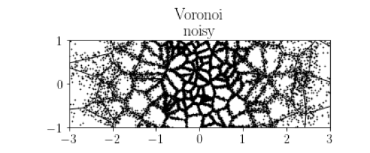
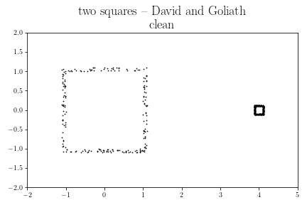
Figure 1: Datasets with small topological features.

However, small holes could be relevant too. For instance, in the toy example on the right of Figure 1, points are sampled from two squares with different sizes and densities. Since the smaller square has a higher density, it may be more relevant than the bigger square. Note that density consideration is crucial in the identification of small holes–in the extreme case, a “small square” formed by only four points is less likely a true hole than four points that happen to be nearby. The aforementioned toy example will be discussed further in Section 4.1. Beyond toy examples, small holes have been found to be relevant in practice too. They could be signs of enclave communities in network analysis stolz17_smallFeatures_networks ; feng21_smallFeatures_voting ; or evidence of fractal structures or high-curvature regions jaquette20_smallFeatures_fractalDimension ; bubenik20_smallFeatures_curvature . Some datasets may only have small holes, or have holes with a wide range of sizes motta18_smallFeatures_hexagonalLattices ; xia14_smallFeatures_protein ; aragoncalvo12_cosmic_void_hierarchy ; wilding21_cosmic_void_TDA . Sometimes small features have better predictive power bendich16_brainArteryTrees .

In the TDA literature, various approaches have been proposed to handle datasets with varying scales, and hence handle their smaller features more fairly. The multi-parameter-persistence approach has gained a lot of attention lately carlsson09_multipersistence ; sheehy12_multicover ; blumberg21_bipersistence_stability ; lesnick15_interactive_bipersistence ; moon18_persistence_terrace . Alternatively, conformal geometry can be used to magnify small holes. For instance, the continuous $k$-NN graph berry19_kNN_graph and density-scaled Vietoris and Cech complexes hickok22_density_scaled_filtration were proposed, and the latter was shown to be stable against uniformly bounded extrinsic perturbation.

In the present work, a novel robust single-parameter scale-invariant approach, called the Robust Density-Aware Distance (RDAD) Filtration is proposed to identify small holes. The proposed method scales the ambient Euclidean distance with density in the sense of Bell et al bell19_weighted_persistence (see berry19_kNN_graph ; hickok22_density_scaled_filtration for conformal interpretations of such scaling) and robustness is ensured by incorporating the concept of distance-to-measure (DTM), which was first proposed in chazal11_DTM and was further studied and generalized in buchet16_DTM_approximation ; chazal18_DTM_statistics ; anai19_DTM_generalizations .

The proposed approach magnifies small holes of dense regions. Under suitable conditions, if a low-density region is surrounded by a high-density region, it gives rise to a homology class whose persistence scales with both a positive power of the density level and the size of the low-density region. Therefore, even if the low-density region is small, its persistence can still be large if the surrounding region has a high enough density. This is made precise in Corollary 3.

The proposed approach is scale-invariant, in the sense that the persistences of all homology classes remain the same when the dataset is uniformly scaled. Therefore, the persistences of the topological features of the dataset are not reduced no matter by how much the dataset is shrunk. This is made precise in Proposition 4.

The proposed approach is robust. If a density is perturbed morderately in the Wasserstein metric and in the sup-norm, then the persistences of all homological features are also perturbed moderately. In particular, the proposed approach is provably robust against additive noise (with possibly unbounded support) and outliers. This is made precise in Theorem 5 and Corollary 6.

These properties will be illustrated through variations of the toy example on the right subplot of Figure 1. The more complicated synthetic dataset on the left subplot will then be studied. We also study a dataset of the locations of American cellular towers.

The rest of the paper is organized as follows. After reviewing the mathematical background in Section 2, we define the proposed filtration in Section 3 and discuss its properties in Section 4. We discuss bootstrapping in Section 5 and present numerical simulations in Section 6. A discussion and the conclusion are presented in Sections 7 and 8. We collect proofs in Appendix A and simulation variables in Appendix B. An implementation of the proposed method is available at https://github.com/c-siu/RDAD.

2 Background

We first review the theory of persistent homology in Section 2.1. In Section 2.2, we discuss the distance filtration, which is the backbone of the traditional TDA approach, as well as various alternatives to the distance filtration, and we will explain their relevance to the present work. We conclude this section with a brief review of the theory of density estimation in Section 2.3.

2.1 Persistent Homology

Persistent homology captures the evolution of the homology of a family of topological spaces. We review general definitions in this subsection and we discuss specific filtrations in the next. We refer the reader to edelsbrunner10comptopo ; otter17_persistent_homology for detailed expositions.

Filtrations and Persistence Diagrams

A filtration is a family $(X_{t})$ of topological spaces such that

$$X_{s}\subseteq X_{t}\text{ whenever }s\leq t.$$

The persistent homology of a filtration $(X_{t})$ is the family of homology groups $(H_{*}(X_{t}))$ along with the maps between them induced by inclusion. Homology classes appear and vanish as the parameter $t$ varies, and the parameters at which they do so are called the birth time and the death time of the class. The class’s persistence is the difference of its birth and death times. The death time is infinite if the class never vanishes.

These birth and death times can be succinctly summarized in persistent diagrams. The $k^{th}$ persistence diagram is a multiset of points in the extended quadrant $[0,\infty)\times[0,\infty]$. The $x$- and $y$-coordinates of each point in this multiset is the birth and death times of a $k$-dimensional homology class.

Stability, Interleaving and Bottleneck Distance

Persistence diagrams are stable against certain perturbations of the filtration. This can be made precise using two similarity measures: the interleaving distance for filtrations and the bottleneck distance for persistence diagrams. Both similarity measures are symmetric and satisfy the triangle inequality. The map from filtrations to persistence diagrams is stable in the sense that the change in the persistence diagrams measured with bottleneck distance is bounded from above by the change in the filtration measured by the interleaving distance. The two similarity measures are defined as follows.

Two filtrations $(X_{t})$ and $(Y_{t})$ are said to be $\varepsilon$-interleaved if

$$X_{t}\subseteq Y_{t+\varepsilon}\text{ and }Y_{t}\subseteq X_{t+\varepsilon}$$ (1)

for every parameter $t$. The interleaving distance of two filtrations is the infimum of all $\varepsilon$’s for which the two filtrations are $\varepsilon$-interleaved.

The bottleneck distance $W_{\infty}(P,Q)$ between persistence diagrams $P$ and $Q$ is the minimal $\Delta\geq 0$ such that there exists a “bijective" pairing of points in $P$ and $Q$ with the sup-norm distance of the points in each pair bounded above by $\Delta$. “Bijective" is in quotes because in general, the two diagrams may not have the same number of points, and excessive points are allowed to be paired with points on the diagonal $\{(x,x):x\in\mathbb{R}\}$. In symbols, we have

$$W_{\infty}(P,Q)=\inf_{\varphi:P\to Q\text{``bijective"}}\sup_{p\in P}\|p-\varphi(p)\|_{\infty}.$$

For points with infinite death time, we adopt the convention that $\infty-\infty=0$ and $\infty-x=\infty$ for $x\in\mathbb{R}$.

The bottleneck distance metric ball is useful for discerning significant features. In fasy14_confidence_set as well as in the present work, a confidence set of persistence diagrams is defined as the bottleneck distance metric ball whose center is the empirical persistence diagram and whose radius $r$ is the significance threshold determined by bootstrapping. A homology class is considered significant if and only if the corresponding point $p$ in the empirical diagram lies above the line $y=x+2r$, where $r$ is the significance threshold obtained by bootstrapping, because any diagram in the ball must have a non-diagonal point paired with the point $p$ in the empirical diagram.

Sublevel Filtration

Given a function $f:X\to\mathbb{R}$ on a topological space $X$, its sublevel filtration consists of the sublevel sets

$$f^{-1}(-\infty,t]=\{x:f(x)\leq t\}$$

of $f$. We often abuse the terminology and identify the sublevel filtration of a function with the function itself. All filtrations in the present work are sublevel filtrations.

Every pair of continuous functions $f,g:X\to\mathbb{R}$ on a compact space $X$ is $\|f-g\|_{L^{\infty}(X)}$-interleaved. Hence functions close together in the sup-norm have similar persistence diagrams. In the present work, all convergence results are locally uniform, and hence the persistence diagrams of the corresponding functions (when restricted to a compact set) become similar.

2.2 Specific Filtrations

The most commonly used filtration is the distance filtration. While it can identify clean global topological signals, it is less useful for small and noisy features. To overcome this, multiple alternatives have been suggested. In this subsection, after briefly discussing the distance filtration, we review Bell et al’s weighted filtration bell19_weighted_persistence and the distance-to-measure filtration chazal11_DTM ; buchet16_DTM_approximation ; chazal18_DTM_statistics ; anai19_DTM_generalizations . The proposed filtration adapts the weighted filtration with density as the weight, and it incorporates the concept of distance-to-measure to enhance robustness.

2.2.1 The Distance Filtration

The distance filtration of a compact set $K$ in a metric space is the sublevel filtration of $d_{K}(x)=\min_{\xi\in K}d(x,\xi)$. If $K$ is finite, the sublevel sets are unions of metric balls, which grow in size as the filtration parameter increases. The distance filtration of data points in a Euclidean space is one of the most commonly used filtrations in topological data analysis. See Figure 2 and its caption for a simple example.

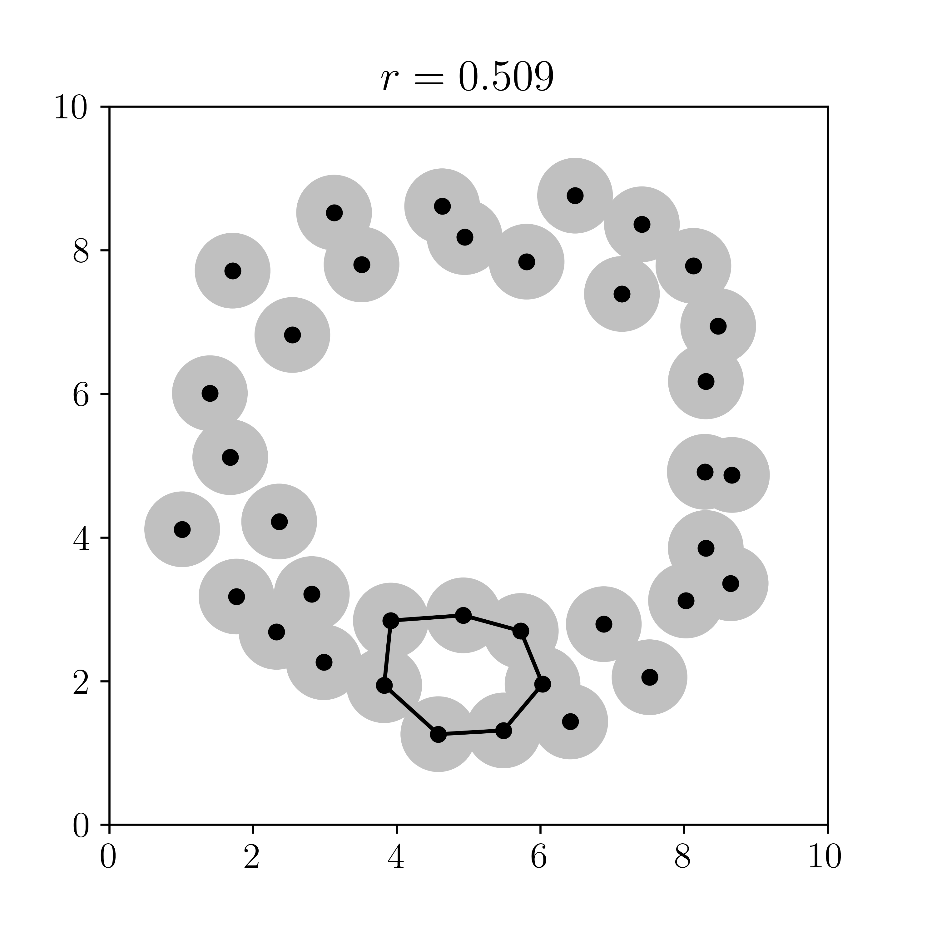
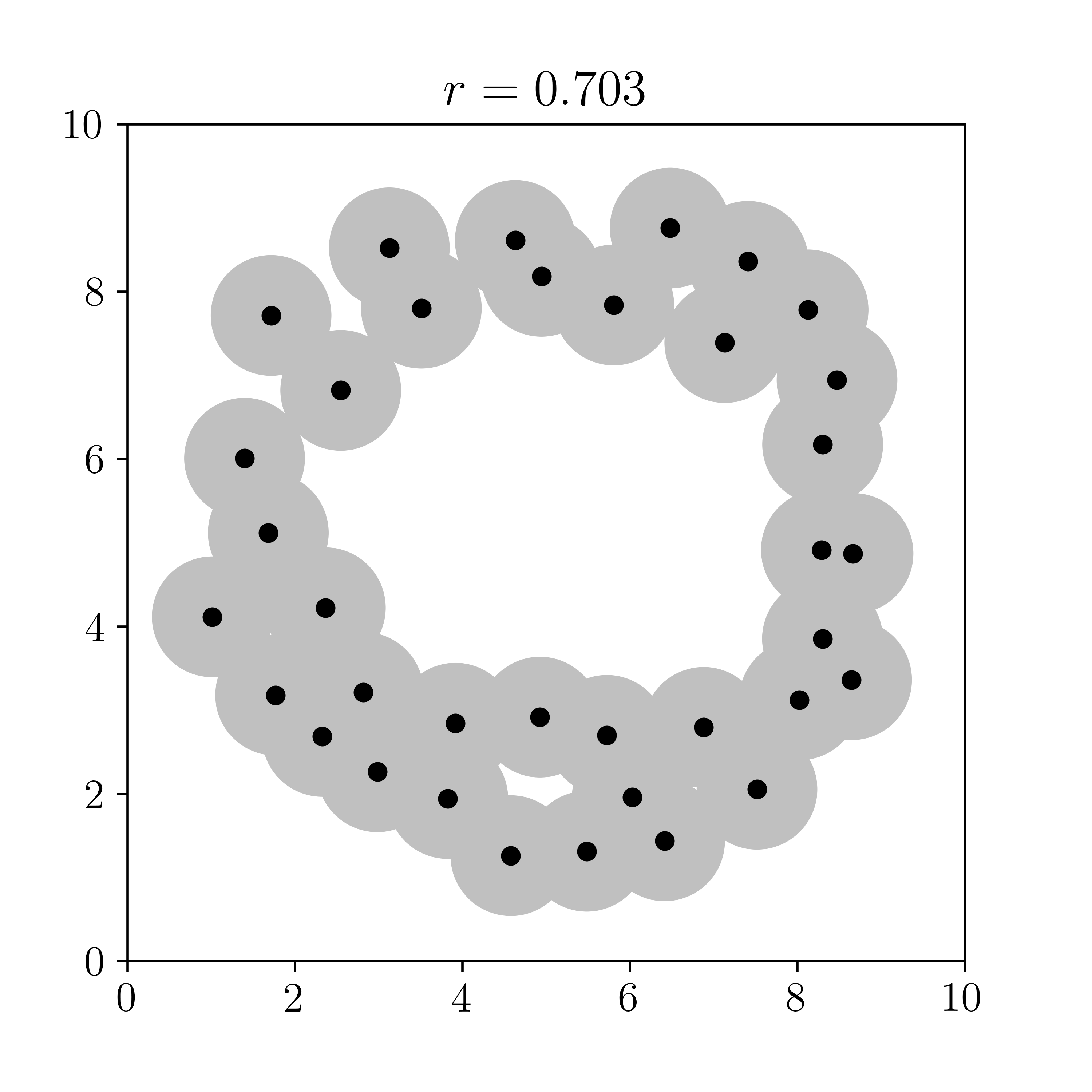
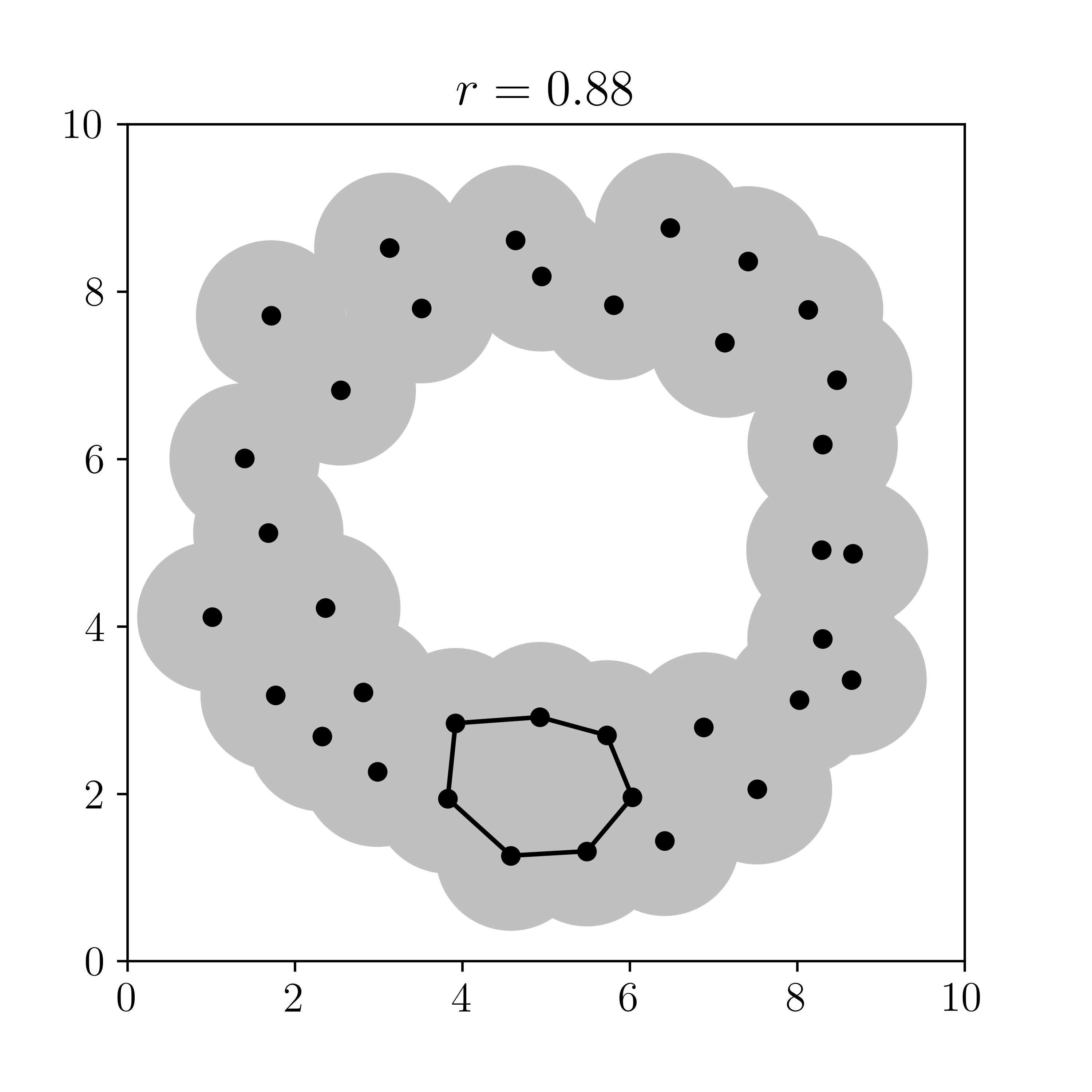
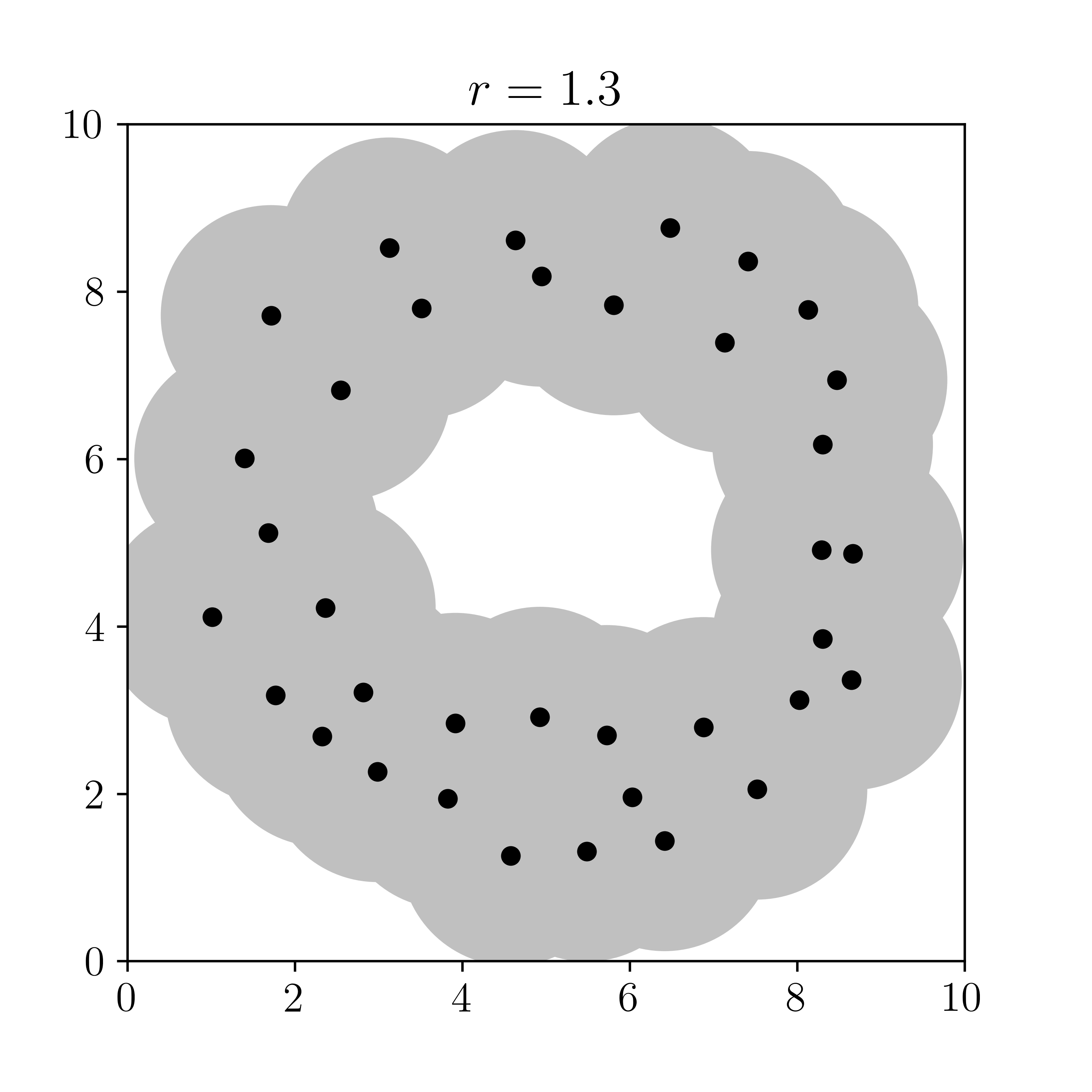
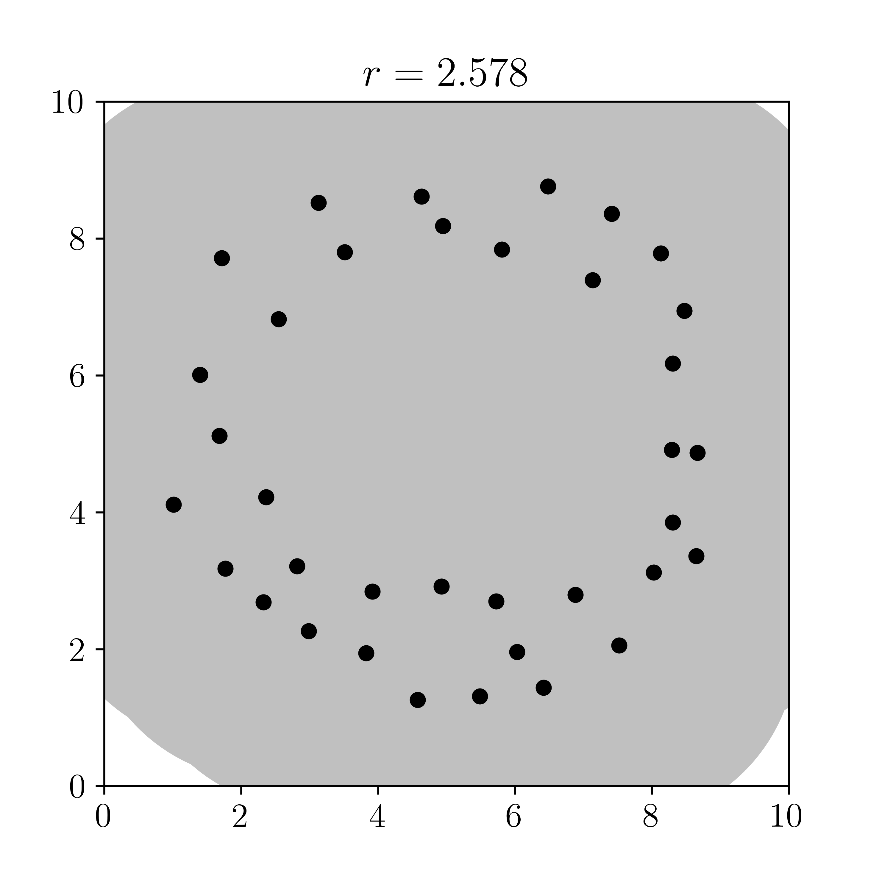
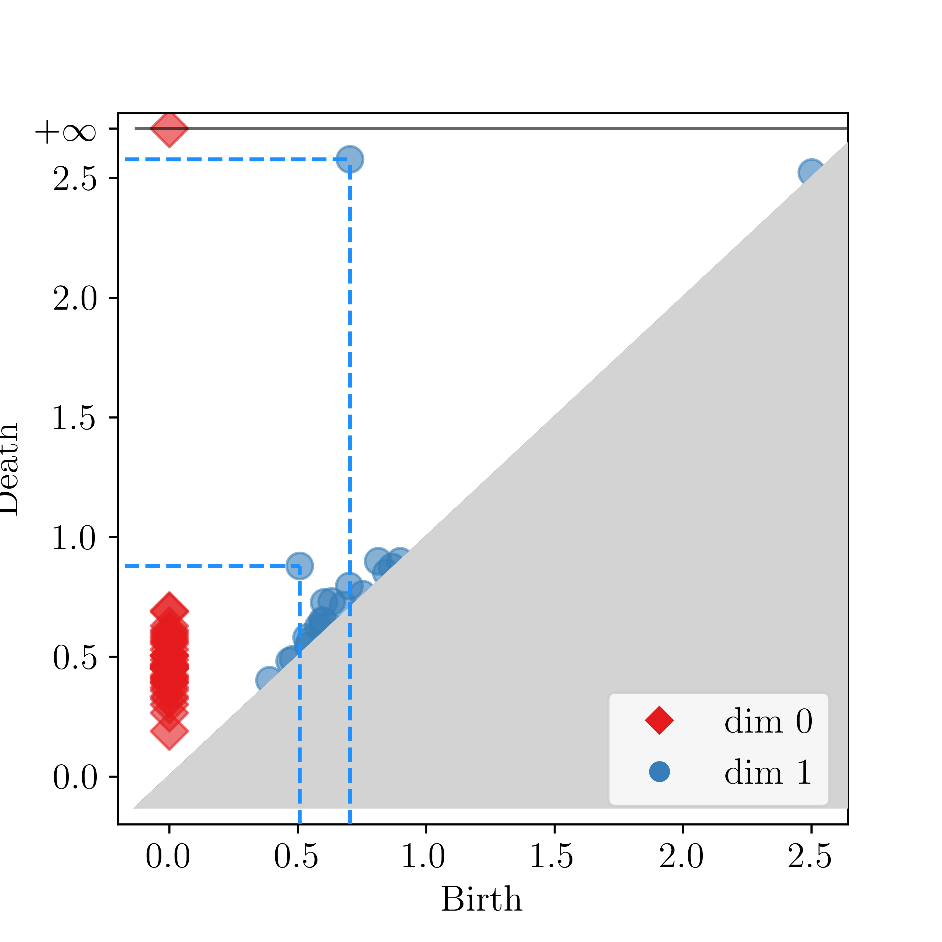
Figure 2: The distance filtration and its persistence diagrams. In the first subplot is a sample of points near a circle. Unions of balls centered at these points with different radii are shown the subsequent subplots. The last subplot shows the persistence diagrams of these unions of balls. The red diamond points correspond to the dimension-0 diagram, and the blue circular points correspond to the dimension-1 diagram. The point marked by dashed lines near the diagonal corresponds to the marked polygon in the third subplot and is filled in the fifth subplot. The marked blue point that is far away from the diagonal corresponds to the main loop that is formed in the fourth subplot and is filled in the second last subplot.

2.2.2 Bell et al’s Weighted Filtration

In bell19_weighted_persistence , a weighted filtration, based on the idea of growing balls at custom rates, is proposed. Given points $\{X_{1},...,X_{N}\}$ and rates $v_{1},...,v_{N}>0$,

$$\hat{V}_{r}=\cup_{i}\bar{B}(X_{i},v_{i}r),$$

is considered. ($\bar{B}(x,s)$ denotes the closed metric ball with center $x$ and radius $s$.) $\hat{V}_{r}$ is the sublevel filtration of the function $\hat{d}_{v}:\mathbb{R}^{D}\to\mathbb{R}$ defined by

$$\hat{d}_{v}(x)=\min_{i}d(x,X_{i})/v_{i}.$$

The number of points needs not be finite. Given $E\subseteq\mathbb{R}^{D}$ and $v:E\to(0,\infty)$, one may consider

$$V_{r}=\overline{\cup_{\xi\in E}B(\xi,v(\xi)r)}.$$

Under mild assumptions, e.g. when there exist constants $v_{1},v_{2}$ such that $0<v_{1}\leq v(\xi)\leq v_{2}<\infty$, $V_{r}$ is the sublevel filtration of

$$d_{v}(x)=\inf_{\xi\in E}d(x,\xi)/v(\xi).$$ (2)

The paper bell19_weighted_persistence establishes various combinatorial properties of the weighted filtration, which will not be needed in the present work, as the proposed filtration is implemented as a cubical filtration.

In the application presented in bell19_weighted_persistence , the rates are chosen to be the pixel intensities of an image, and applications to noisy datasets are alluded to. In the present work, we will specialize to the case when $v$ is a function of the density from which the sample points $X_{1},...,X_{N}$ are drawn. However, the direct adaptation struggles with low-density regions, and hence is not robust against noise and outliers, as we will see in the simulations in Section 4.3. To develop a more nuanced approach for handling low-density regions, we borrow the idea of distance-to-measure.

2.2.3 Distance-to-Measure (DTM) Filtration and Robustness

The distance-to-measure (DTM) function is a modification of the distance function that is designed to enhance robustness against potential noise and outliers. Roughly speaking, the distance-to-measure of a point $x$ to a probability measure $\mu$ is the average distance of $x$ from the nearest part of the support that carries sufficient mass. As opposed to the distance to the support of $\mu$, it is not estimated by a minimum. Rather, it is averaged over a positive mass, and hence it is more robust. The distance-to-measure filtration is the sublevel filtration of the distance-to-measure function.

Formally, the distance-to-measure function of a probability measure $\mu$ on $\mathbb{R}^{D}$, with parameter $0<m<1$, is defined by

$$DTM(x)=DTM(x\mathchar 24635\relax\;\mu,m)=\sqrt{\frac{1}{m}\int_{0}^{m}G_{x}^{-1}(q)^{2}dq},$$ (3)

where $G_{x}^{-1}$ is the generalized inverse function of

$$G_{x}(r)=\mu[\bar{B}(x,r)].$$ (4)

$G_{x}^{-1}(q)$ may be seen as the $q^{th}$ quantile of the distribution of $d(x,X)$, where $X$ is a random vector with distribution $\mu$.

When the probability measure takes the form $\hat{\mu}=\frac{1}{N}\sum_{i=1}^{N}\delta_{X_{i}}$, where $\delta_{x}$ denotes the dirac delta measure at $x$, and $m=k_{\text{DTM}}/N$ for some positive integer $k_{\text{DTM}}$ smaller than $N$, the function takes the form

$$DTM(x\mathchar 24635\relax\;\hat{\mu},k_{\text{DTM}}/N)=\sqrt{\frac{1}{k_{\text{DTM}}}\sum_{i=1}^{k_{\text{DTM}}}d(x,X_{(i)})^{2}},$$ (5)

where $X_{(i)}$ is the $i^{th}$ nearest neighbor to $x$ among $X_{1},...,X_{N}$.

When $k_{\text{DTM}}=1$, we recover the distance function to the set $\{X_{1},...,X_{N}\}$ as a special case. The distance-to-measure function is more robust against noise and outliers than the plain distance function because it takes into account not just the nearest neighbor, which may be an outlier, but additional points as well.

In the present work, this idea will be used to enhance the robustness of the weighted filtration.

2.3 Density Estimation by Nearest Neighbors

For a filtration $(Y_{t})$ defined in terms of a density function $f$, we must first estimate $f$ before we can estimate the persistence homology of $(Y_{t})$ from a dataset drawn from $f$. Common density estimation methods include the kernel method and the nearest neighbor method. The latter is used in the proposed filtration because it adapts the amount of smoothing to the local density. We refer the reader to silverman_density for the theory of density estimation, and biau_devroye_nearest_neigbhor for the nearest neighbor approach.

The nearest-neighbor density estimate based on a sample $\{X_{1},...,X_{N}\}\subseteq\mathbb{R}^{D}$ is defined by

$$\hat{f}_{k}(x)=\hat{f}_{k}(x\mathchar 24635\relax\;X_{1},...,X_{N},k)=\frac{k}{N}\frac{1}{\omega_{D}d_{k}(x)^{D}},$$ (6)

where $\omega_{D}$ is the volume of the unit ball in $\mathbb{R}^{D}$ and $d_{k}(x)$ is the distance from $x$ to the $k^{th}$ nearest neighbor of $x$ among the points $X_{1}$, …, $X_{N}$, i.e.

$$d_{k}(x)=d(x,X_{i_{k}}),\text{ where}$$

$$d(x,X_{i_{1}})\leq d(x,X_{i_{2}})\leq...\leq d(x,X_{i_{N}}).$$

The estimate Equation 6 is motivated by the local approximation

$$\frac{k}{N}\approx\int_{B(x,d_{k}(x))}f(y)dy\approx f(x)\lvert B(x,d_{k}(x))\rvert=f(x)\omega_{D}d_{k}(x)^{D},$$

where $\lvert\cdot\rvert$ denotes the Lebesgue measure, and $f$ is the true density of the independent and identically distributed sample $\{X_{1},...,X_{N}\}$.

The first approximation applies when $N$ is large, since the empirical measure of the ball approximates its true measure. The second approximation applies when $f$ is smooth enough near $x$ and when $d_{k}(x)$ is small.

3 Proposed Filtration

We define the proposed filtration and its estimator in this section.

Definition 1 (Population RDAD).

Let $f$ be a density on $\mathbb{R}^{D}$ and $P$ be the measure induced by $f$. Let $m\in(0,1)$. The population robust density-aware distance function $RDAD$ is defined by

$$RDAD(x) =RDAD(x\mathchar 24635\relax\;f,m)$$

$$=\sqrt{\frac{1}{m}\int_{0}^{m}F_{x}^{-1}(q)^{2}dq},$$ (7)

where

$$F_{x}(r)=P\left[f(X)^{1/D}d(X,x)\leq r\right].$$ (8)

For the sake of comparison, the Density-Aware Distance ($DAD$) function, which has been shown to be not robust against noise and outliers in hickok22_density_scaled_filtration , is defined as follows.

Definition 2 (Population DAD).

Let $f$ be a density on $\mathbb{R}^{D}$ and $P$ be the measure on $\mathbb{R}^{D}$ induced by $f$. The population density-aware distance function $DAD$ is defined by

$$DAD(x)=\text{ess-}\inf_{y\in\mathbb{R}^{D}}d(x,y)f(y)^{1/D},$$ (9)

where $\text{ess-}\inf$ denotes the essential infimum with respect to the measure $P$.

One may check that the DAD function is Bell et al’s weighted filtration with $1/f(x)^{1/D}$ as the growth rates of metric balls, and RDAD is the DAD function made robust using the DTM idea. Intuitively, weighting by the density slows down ball growth in high-density regions, so that persistences of homology classes of those regions are prolonged. We make this idea precise in Section 4.1.

We now introduce an empirical version of the RDAD function and the DAD function that are defined in terms of a sample $\{X_{1},...,X_{N}\}\subseteq\mathbb{R}^{D}$. The empirical RDAD is defined by combining the distance-to-measure function Equation 5 for the discrete measure $\frac{1}{N}\sum_{i=1}^{N}\delta_{X_{i}}$ in Section 2.2.3 and the nearest neighbor density estimator. This requires two parameters, $k_{\text{DTM}}$ and $k_{\text{den}}$. The former is needed to set $m=k_{\text{DTM}}/N$, and the latter is the number of nearest neighbors used for density estimation. One gets the empirical DAD function by putting $k_{\text{DTM}}=1$.

Let $X_{1},...,X_{N}\in\mathbb{R}^{D}$, and for each $i=1,...,N$, let $d_{i}$ be the distance from $X_{i}$ to its $k_{\text{den}}^{th}$-nearest neighbor among $X_{1},....,X_{N}$.

Definition 3 (Empirical DAD and RDAD).

Let $k_{\text{DTM}},k_{\text{den}}$ be positive integers strictly less than $N$. For each $x\in\mathbb{R}^{D}$, let $d(x,X_{(i)})/d_{(i)}$ be the $i^{th}$ order statistic of $d(x,X_{1})/d_{1}$,…, $d(x,X_{N})/d_{N}$. The empirical (robust) density-aware distance functions $\widehat{DAD}$ and $\widehat{RDAD}$ are defined by

$$\widehat{DAD}(x) =\widehat{DAD}(x\mathchar 24635\relax\;X_{1},...,X_{N},D,N,k_{\text{den}})$$

$$=\min_{i}d(x,X_{i})\hat{f}_{k_{\text{den}}}(X_{i})^{1/D}$$ (10)

$$=\min_{i}C_{N,k_{\text{den}},D}d(x,X_{i})/d_{i}$$

$$\widehat{RDAD}(x) =\widehat{RDAD}(x\mathchar 24635\relax\;X_{1},...,X_{N},D,N,k_{\text{den}},k_{\text{DTM}})$$

$$=C_{N,k_{\text{den}},D}\sqrt{\frac{1}{k_{\text{DTM}}}\sum_{i=1}^{k_{\text{DTM}}}(d(x,X_{(i)})/d_{(i)})^{2}}$$ (11)

where $C_{N,k_{\text{den}},D}=\left(\frac{1}{\omega_{D}}\frac{k_{\text{den}}}{N}\right)^{1/D}$ and $\omega_{D}$ is the volume of the unit ball in $\mathbb{R}^{D}$.

4 Properties

In this section, we present certain desirable properties of the proposed filtration and substantiate our claims in the introduction. In Section 4.1, we discuss how the proposed filtration prolongs persistences of homology classes of high-density regions. Then we discuss, in Section 4.2, the proposed filtration’s scale invariance, which motivates the awkward-looking exponent $1/D$ in the definition of the RDAD function, and in Section 4.3, its robustness, which is enhanced by the DTM setup. We conclude by giving further mathematical properties of the proposed filtration in Section 4.4. All proofs are delayed to Appendix A.

4.1 Prolonged Persistence for High-Density Regions

In this subsection, we illustrate how the proposed filtration prolongs persistences of homology classes of high-density regions with a numerical example, and we formalize the observations from the example with theorems. For the numerical examples in this and subsequent subsections, parameters are summarized in Table 3 in Appendix B, and implementation details are deferred to Section 6.1.

4.1.1 Example

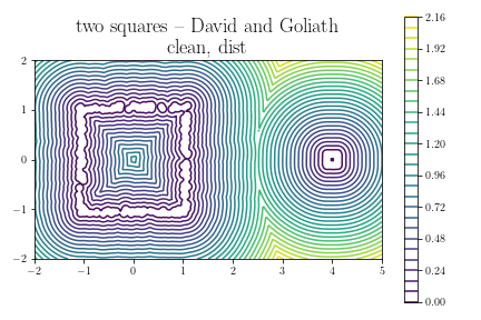
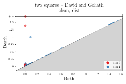
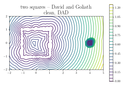
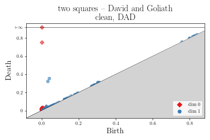
Figure 3: Contour plots and persistence diagrams of different filtrations for the “David and Goliath" two-square dataset.

Recall the two-square dataset “David and Goliath" in the right subplot of Figure 1 in the introduction. 100 points are uniformly sampled from the bigger square annulus, and 400 from the smaller annulus. Since the dataset has no additive noise or outliers, we compare the distance filtration and the DAD filtration for this dataset. Their contour plots and persistence diagrams are shown in Figure 3. The plots and the diagrams for DTM and RDAD are similar to the distance and DAD figures correspondingly.

Two squares are clearly visible in the scatter plot in the right subplot of Figure 1. However, the blue point corresponding to the smaller square in the persistence diagram of the distance filtration is very close to the diagonal (it is at the tip of the cluster of red diamonds near the origin). On the other hand, for the DAD filtration, two blue circular points in the persistence diagrams are comfortably far away from the diagonal. The contour plot of the DAD function explains this: the dense contour lines inside the small square, due to the higher density on the smaller annulus, show the smaller square hole does not get filled over a wide range of levels. This shows that the proposed choice of weights prolongs the persistence of homology classes of high-density regions.

4.1.2 Setup and Assumptions

We need the following setup for formal statements.

• $f:\mathbb{R}^{D}\to[0,\infty)$ is a bounded probability density function, and $P$ is the probability measure induced by $f$.

• $0\leq t_{0}\leq...\leq t_{k}\leq\|f\|_{\infty}$ and for each $i$, $\Omega_{i}$ is a connected component of $f^{-1}[t_{i},\infty)$. The $\Omega_{i}$’s are pairwise disjoint.

• $s_{i}=\min_{j\neq i}\frac{d(\Omega_{i},\Omega_{j})}{t_{i}^{-1/D}+t_{j}^{-1/D}}$.

For the two-square example above, the points are sampled from a piecewise constant density supported on the two square annuli, which we may take to be $\Omega_{1}$ and $\Omega_{2}$.

We also need the following mass concentration conditions.

Global Condition

$P(\mathbb{R}^{D}-\cup\Omega_{i})\leq m/2$.

Local Condition

There exist $a>1$ and $\rho_{m}>0$ such that for every $x\in\cup\Omega_{i}$,

$$P(B(x,\rho_{m})\cap f^{-1}[0,af(x)])\geq m.$$ (12)

It is not difficult to check that, for an $L$-Lipscthiz density $f$, if $m$ is much smaller than $\left(\frac{t_{0}}{\max(L,1)}\right)^{1/D}$, the local condition is satisfied for any $a$ when one set

$$\rho_{m}\sim\left(\frac{m}{\omega_{D}t_{0}}\right)^{1/D}\sim m^{1/D}.$$

Finally, we also assume $f\mid\partial\Omega_{i}=t_{i}$ for each $i$. Note that this condition and the local mass concentration condition above both concern pointwise function values of the density function $f$, which is only defined up to a set of measure zero. We adopt the convention that these conditions hold as long as they both hold for a function that is almost everywhere equal to $f$.

4.1.3 Results

All results of this section assume the setup laid out above.

We first show that the RDAD function is similar to the DAD function corresponding to a piecewise constant approximation of the density $f$. Let

$$g_{i}(x) =t_{i}^{1/D}d(x,\Omega_{i}),\quad i=1,...,k$$

$$g(x) =\min_{i=1,...,k}g_{i}(x).$$

In the example, since the density is piecewise constant, $g$ is precisely $DAD$. Note that a sublevel set of $g_{i}$ is a neighborhood of $\Omega_{i}$ consisting of $\Omega_{i}$ and a surrounding band whose width is proportional to $1/t_{i}^{1/D}$. Hence, if $t_{i}$ is large, then persistences of homology classes in the filtration $g_{i}$ are prolonged by a factor of $t_{i}^{1/D}$. This remains true for $g$ as long as the filtration level is smaller than $s_{i}/t_{i}^{1/D}$, because the sublevel set of $g$ of each level is the disjoint union of the sublevel sets of the $g_{i}$’s at the level.

Theorem 1.

For every $x\in\mathbb{R}^{D}$,

$$\frac{1}{\sqrt{2}}g(x)\leq RDAD(x\mathchar 24635\relax\;f,m)\leq a^{1/D}g(x)+O(\rho_{m}),$$

where the big-Oh constant depends only only on $\|f\|_{\infty},t_{0},D,a$.

Corollary 2.

Every homology class in the distance filtration of $\Omega_{i}$ with birth and death times $\beta$ and $\delta$ induces a class in the RDAD filtration with persistence at least

$$t_{i}^{1/D}(\frac{1}{\sqrt{2}}\delta-a^{1/D}\beta)-O(\rho_{m})$$

whenever $t_{i}^{1/D}\delta<s_{i}$.

In particular, if the difference in the parentheses in the corollary is positive and $\rho_{m}$ is small, then the persistence is scaled roughly by a factor of $t_{i}^{1/D}$.

Returning to the central claim that the RDAD filtration highlights low-density regions surrounded by high-density regions, the above corollary combined with Alexander duality gives the following result at dimension $D-1$.

Corollary 3.

Suppose $f$ is $C^{1}$-smooth and $t_{i}$ is not a critical value of $f$. Let $M$ be a bounded connected component of the complement of $\Omega_{i}$ and $r=\max_{x\in M}d(x,\partial M)$. Then $\partial M$ determines a $(D-1)$-dimensional homology class in the RDAD filtration with persistence at least

$$\frac{1}{\sqrt{2}}t_{i}^{1/D}r-O(\rho_{m})$$

whenever $t_{i}^{1/D}r<s_{i}$.

In the corollary, $M$ is a low-density region that is surrounded by the high-density region $\Omega_{i}$. Its boundary induces a $(D-1)$-homology class in the RDAD filtration whose persistence is at least a quantity that scales with a positive power of the density level and $r$, which measures the size of the low-density region $M$. Hence, if the density threshold $t_{i}$ or the size $r$ of $M$ is big, and the other factor is moderate, the persistence will be long as long as $\rho_{m}$ is not too big.

In the two-square example, $M$ could be the square inside the small annulus, and $r$ is the half the sidelength of $M$.

4.2 Scale Invariance

While many other choices of growth rates may prolong the persistences of small features, our specific choice makes the filtration scale-invariant. This means that uniformly scaling a dataset does not change the persistence diagrams. In particular, no matter by how much a dataset is shrunk, its topological features still have the original persistences. Precisely, we have the following proposition.

Proposition 4 (Scale invariance).

Let $a>0$ and $b\in\mathbb{R}^{D}$ be constants.

Population version:

Let $X$ be a random vector in $\mathbb{R}^{D}$ with density $f$. Let $\tilde{X}=aX+b$ and $\tilde{f}$ the density of $\tilde{X}$. Then for any $0<m<1$,

$$RDAD(ax+b\mathchar 24635\relax\;\tilde{f},m)=RDAD(x\mathchar 24635\relax\;f,m),$$

and hence the $RDAD(\;\cdot\;\mathchar 24635\relax\;\tilde{f},m)$ and $RDAD(\;\cdot\;\mathchar 24635\relax\;f,m)$ have the same persistence diagrams.

Sample version:

Let $X_{1},...,X_{N}$ be points in $\mathbb{R}^{D}$, and let $\tilde{X}_{i}=aX_{i}+b$. Then for any positive integer $k_{\text{DTM}}$ strictly less than $N$,

$$\widehat{RDAD}(ax+b\mathchar 24635\relax\;\tilde{X}_{1},...,\tilde{X}_{N},D,N,k_{\text{den}},k_{\text{DTM}})$$

$$\qquad=\widehat{RDAD}(x\mathchar 24635\relax\;X_{1},...,X_{N},D,N,k_{\text{den}},k_{\text{DTM}}),$$

and hence the two $\widehat{RDAD}$ filtrations have the same persistence diagrams.

Theorem 5 of hickok22_density_scaled_filtration is a conformal analogue of this result.

We illustrate the scale invariance property with the “Antman" example in Figure 4. The same number of points are sampled randomly from two square annuli, which are scaled versions of each other. Thus, the two square holes give two nearby (overlapping) blue circular points in the persistence diagrams in Figure 4.

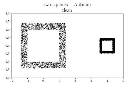
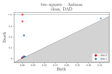
Figure 4: Sample points of the “Antman" two-square dataset, and the persistence diagram of the empirical DAD filtration for this dataset

4.3 Robustness

The RDAD filtration is designed to be robust against additive noise and outliers. Indeed, Theorem 5 below shows that the RDAD function is only mildly perturbed if the perturbation of $f$ is small in both the Wasserstein metric and the sup-norm relative to the parameter $m$. In particular, Corollary 6 shows the perturbation is mild in the presence of additive noise and outliers.

We need the following notations and terminologies.

Wasserstein distance

By the order-$p$ Wasserstein distance $W_{p}(f,\tilde{f})$ between two densities $f,\tilde{f}$, we mean the order-$p$ Wasserstein distance between the measures they induce.

Moment

By the $p^{th}$ moment $M_{p}$ of a random vector $X$ we mean $M_{p}=E[\lvert{X}\rvert^{p}]$. Moments of density functions and measures are defined analogously.

Moderate Tail

A random vector $X$ in $\mathbb{R}^{D}$ is said to have a moderate tail with parameters $C,\alpha>0$ if $P(\lvert{X}\rvert>R)\leq CR^{-\alpha}$. The notion of moderate tails for density functions and measures are defined analogously.

We are now ready to state our stability result.

Theorem 5 (Stability).

Let $2<p\leq\infty$, and let $f$ and $\tilde{f}$ be densities on $\mathbb{R}^{D}$. Suppose $f$ and $\tilde{f}$ have finite $q^{th}$ moments for every $q\in[1,\infty)$ and they have moderate tails with parameters $C,\alpha>0$, where $\alpha\geq D^{2}-D$. Suppose further that $f^{1/D}$ is Lipschitz and bounded. If $2<r<p$, $W_{p}(f,\tilde{f})\leq 1$ and $\|f-\tilde{f}\|_{\infty}\leq 1$, then for any $0<m<1$ and every compact set $K$,

$$\|RDAD(\;\cdot\;\mathchar 24635\relax\;f,m)-RDAD(\;\cdot\;\mathchar 24635\relax\;\tilde{f},m)\|_{L^{\infty}(K)}=\frac{1}{m^{1/r}}O(W_{p}(f,\tilde{f})+\|f-\tilde{f}\|_{\infty}^{\frac{D+r}{(D+1)(r+1)}}),$$

where the big-Oh constant depends only on $f,D,K,C,p,r$ and the moments of $f$ and $\tilde{f}$.

To model additive noise and outliers, let $X,Y^{\text{add}}$ and $Y^{\text{out}}$ be random vectors in $\mathbb{R}^{D}$, with densities $f,g^{\text{add}}$ and $g^{\text{out}}$; and let $Z$ be a Bernoulli random variable with success probability $\delta\in[0,1)$. Let $\varepsilon\in[0,1)$. Suppose $X,Y^{\text{add}},Y^{\text{out}}$ and $Z$ are independent. We model a corrupted $X$ by considering

$$\tilde{X}=(1-Z)(X+\varepsilon Y^{\text{add}})+ZY^{\text{out}}.$$

Corollary 6.

Suppose $X,Y^{\text{add}}$ and $Y^{\text{out}}$ have $q^{th}$ moments for every $q\in[1,\infty)$ and they have moderate tails with parameters $C,\alpha>0$, where $\alpha\geq D^{2}-D$. Suppose $f^{1/D}$ is Lipschitz and bounded, and $g^{\text{out}}$ is bounded. Then for any $r\in(2,\infty)$,

$$\|RDAD(\;\cdot\;\mathchar 24635\relax\;f,m)-RDAD(\;\cdot\;\mathchar 24635\relax\;\tilde{f},m)\|_{L^{\infty}(K)}=\frac{1}{m^{1/r}}O(\delta^{1/(r+1)}+\varepsilon^{\frac{D+r}{(D+1)(r+1)}}),$$

where the big-Oh constant depends only on $f,D,K,C,r$, moments of $f,g^{\text{add}}$ and $g^{\text{out}}$, and their sup norms as functions on $\mathbb{R}^{D}$.

The DTM analogue of this theorem is Lemma 4 of chazal18_DTM_statistics . Our proof loosely follows the argument there but there are considerable complications owing to the asymmetry of the definition of RDAD.

We illustrate the results above with corrupted versions of the “Antman" example in Figure 5. We compare the DAD filtration and the RDAD filtration in Figures 6 and 7. The persistence diagrams of RDAD for the corrupted datasets are affected to a lesser extent by the noise and outliers than those of DAD.

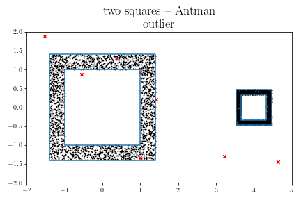
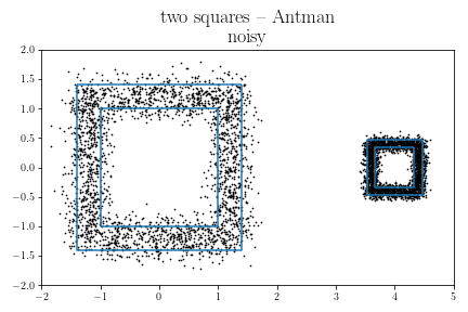
Figure 5: Sample points of corrupted “Antman" two-square datasets (by outliers and by additive noise).

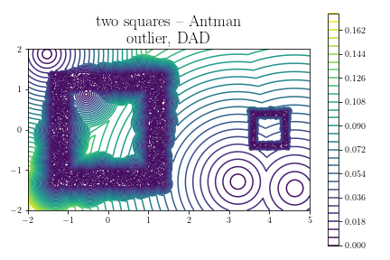
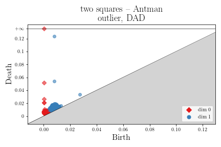
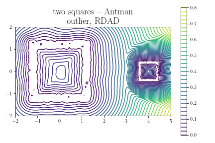
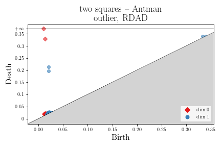
Figure 6: Contour plots and persistence diagrams of different filtrations for the outlier-contaminated “Antman" two-square dataset.

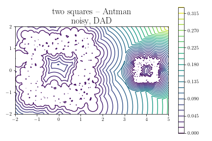
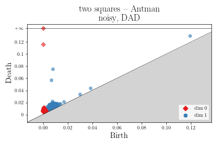
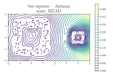
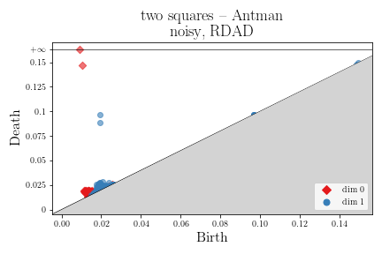
Figure 7: Contour plots and persistence diagrams of different filtrations for the additive noise-contaminated “Antman" two-square dataset.

4.4 Further Properties

We present basic mathematical properties of the proposed filtration in this subsection.

The first result extends Theorem 3.2 in chazal18_DTM_statistics and shows RDAD is indeed an approximation of the DAD function.

Proposition 7 (RDAD as an Approximation of DAD).

Given a density $f$, $RDAD(x\mathchar 24635\relax\;f,m)\to DAD(x\mathchar 24635\relax\;f)$ pointwise as $m\to 0$. The convergence is uniform on every compact set $K$ if $f$ is bounded.

The next lemma is useful for establishing results in previous subsections. It extends Proposition 3.3 of chazal11_DTM .

Lemma 8 (Variational Characterization).

For each $x\in\mathbb{R}^{D}$,

$$m\cdot RDAD(x)^{2}=\min_{\begin{subarray}{c}\nu(\mathbb{R}^{D})=m\\ \nu\text{ subordinate to }P\end{subarray}}\int[f(\xi)^{1/D}d(\xi,x)]^{2}d\nu(\xi),$$

where a measure $\nu$ is said to be subordinate to $P$ if $0\leq\nu(E)\leq P(E)$ for every measurable set $E$. The minimum is attained by definition.

Lipschitz continuity of RDAD ensures that it can be numerically approximated. Its DTM analogue is Theorem 3.1 of chazal18_DTM_statistics .

Proposition 9 (Lipschitz Continuity).

For $2<p<\infty$, if $f\in L^{1+p/D}(\mathbb{R}^{D})$, then $RDAD$ is $[\frac{1}{m^{1/p}}\|f\|_{L^{1+p/D}}^{1/p+1/D}]$-Lipschitz continuous. If $f$ is bounded, then both $DAD$ and $RDAD$ are $\|f\|_{\infty}^{1/D}$-Lipschitz.

Finally we present a statistical convergence result that extends Theorem 9 of chazal18_DTM_statistics .

Proposition 10 (Functional Normality).

Suppose $X_{1},...,X_{N}$ is an independent and identically distributed sample with a density $f$ that is continuous and has a compact support. If $\frac{k_{\text{den}}}{\log N}\to\infty$, $\frac{k_{\text{den}}}{N}\to 0$ and $\frac{k_{\text{DTM}}}{N}\to m$, then on every compact set $K$ in $\mathbb{R}^{D}$, $\sqrt{N}(\widehat{RDAD}^{2}-RDAD^{2})$ converges weakly in $L^{\infty}(K)$ to a centered Gaussian process with covariance kernel

$$\kappa(x,y)=\frac{1}{m^{2}}\int_{0}^{(F_{x}^{-1}(m))^{2}}\int_{0}^{(F_{y}^{-1}(m))^{2}}\left(P(E_{x,t}\cap E_{y,s})-F_{x}(\sqrt{t})F_{y}(\sqrt{s})\right)dsdt,$$

where $E_{z,r}=\{\xi:f(\xi)^{1/D}d(z,\xi)\leq\sqrt{r}\}$ for every $z\in\mathbb{R}^{D}$ and $r>0$.

5 Bootstrapping

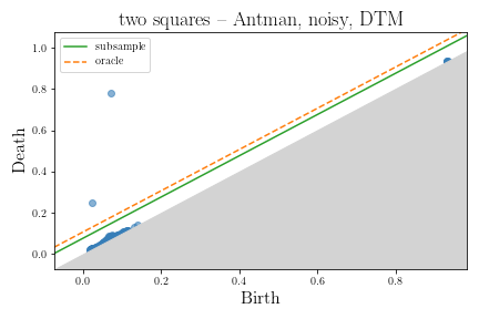
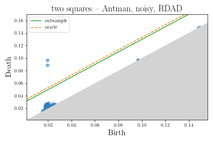
Figure 8: Dimension-1 persistence diagrams of different filtration functions for the additive noise-corrupted “Antman" two-square dataset with confidence bands. Blue points are points in the dimension-1 empirical persistence diagram. The green solid lines and the orange dashed lines are the confidence bands constructed by subsample and oracle bootstrapping respectively.

In order to distinguish statistically significant topological signals from noise, a confidence band like those in fasy14_confidence_set ; chazal18_DTM_statistics is desirable. Below, we discuss how to construct such a confidence band, and compare the resultant band with what an “oracle", who knows the density $f$ from which the points are sampled, would construct. We show that the two bands are empirically similar in the additive noise-corrupted “Antman” example. A more complicated example will be considered in Section 6.2.

Let $\hat{P}$ be the empirical persistence diagram. The confidence set we construct is a bottleneck metric ball centered at $\hat{P}$. Even though an “oracle" who knows the density $f$ would, presumably, know the significant features, we still imagine that they will simply determine an appropriate radius for the ball around the empirical persistence diagram by sampling a certain number of independent samples of the same size from $f$, and approximating, by the empirical quantile, the true $(1-\alpha)$-quantile of the bottleneck distance from $\hat{P}$ to a persistence diagram from an independent sample from $f$. If the original sample has been corrupted, the oracle samples are corrupted by the same mechanism too.

The density $f$ is not known to a “non-oracle". In this case, we adapt the subsampling method proposed in chazal18_DTM_statistics . Specifically, we generate $B$ samples ($B=100$ in our implementation) of $N$ random vectors drawn from $X_{1},...,X_{N}$ with replacement and compute $B$ persistent diagrams $P^{*}_{1},...,P^{*}_{B}$. The radius of the confidence set is the empirical $(1-\alpha)$-quantile of the bottleneck distances of $\hat{P}$ from the $P^{*}_{i}$’s.

In fasy14_confidence_set , each bootstrap sample contains $o(N)$ points. However, since the scale of the proposed filtration changes with the sample size, we fix the bootstrap sample size to be $N$ to ensure comparability of the bootstrap sample and the empirical sample.

Consider, again, the additive noise-corrupted “Antman” two-square dataset on the right of Figure 5. The persistence diagrams for the distance-to-measure filtration and the RDAD filtration are shown in Figure 8 with different confidence bands. Note that in both figures the bands constructed by oracle bootstrapping and by subsample bootstrapping are very close to each other, and both of them identify correctly the two true loops.

6 Simulations

We illustrate the utility of the proposed filtration on synthetic and real data including a brief description of the computation of the persistent diagrams of the empirical $\widehat{RDAD}$ filtration.

First, in Section 6.2, motivated by the multiscale nature of the cosmic web, we attempt to identify Voronoi cells with a range of sizes from observed sample points on cell edges.

Then, in Section 6.3 we attempt to apply our method to a dataset of cellular towers in the United States to discover mesoscale holes formed by geography and missing data.

Model parameters and sample sizes of different datasets are summarized in the tables in Appendix B.

6.1 Implementation

We approximate the empirical $\widehat{RDAD}$ function by a function that is piecewise constant on a fine grid and coincides with the $\widehat{RDAD}$ function at the center of each grid cell. This produces a cubical filtration. We use the implementation in gudhi_CubicalComplex . This computation is feasible for 2- to 3-dimensional data, but we confine ourselves to 2-dimensional data for easier visualization. A byproduct of computing with cubical filtrations is that we can locate the pixel at which each codimension-1 hole is eventually filled.

All homological computations are done with coefficients in $\mathbb{Z}/{11\mathbb{Z}}$, which is the default field in gudhi_CubicalComplex .

6.2 Recovery of Synthetic Voronoi Cells

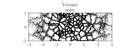
Figure 9: Sample points of the noisy Voronoi dataset.

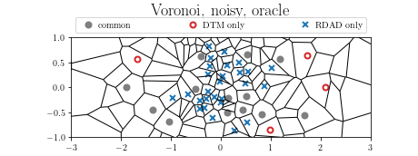
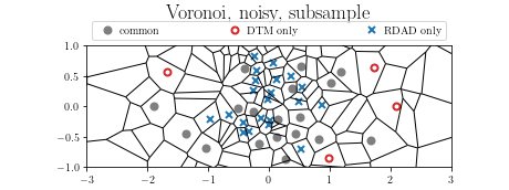
Figure 10: Significant loops under different filtrations and different bootstrapping methods for the noisy Voronoi dataset. Significant loops under different filtrations but the same bootstrapping methods share the same plot and are distinguished by their colors and markers.

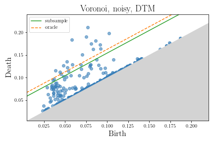
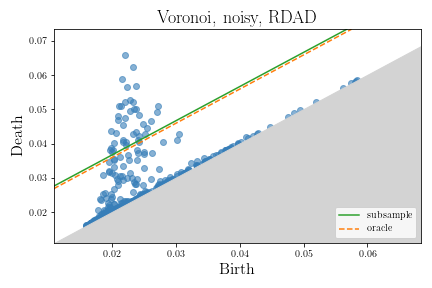
Figure 11: Dimension-1 persistence diagrams of different filtration functions for the noisy Voronoi dataset with confidence bands. Blue points are points in the dimension-1 empirical persistence diagram. The green solid lines and the orange dashed lines are the confidence bands constructed by subsample and oracle bootstrapping respectively.

In this subsection, we attempt to recover the Voronoi cells with the proposed filtration from a sample of points near edges of a planar Voronoi diagram with cells of different sizes and different densities on their edges. This is the same dataset as the one on the left of Figure 1, and it is motivated by the cosmological Voronoi model in icke91_cosmic_void_voronoi (see also pranav16_cosmic_void_TDA ; xu19_cosmic_void_TDA ), where galactic matter is concentrated on walls and filaments of a Voronoi diagram, whose cell sizes span a wide range of scales, as observed in aragoncalvo12_cosmic_void_hierarchy ; wilding21_cosmic_void_TDA . For easier visualization, we consider only planar Voronoi diagrams.

We experiment with Voronoi diagrams in which the cells in the center of the diagram tend to be smaller. A point is sampled by first choosing a random cell and then choosing a uniform point on its boundary. This results in a higher sampling density on boundaries of smaller cells. We further inject additive noise. Further details of the data generation process may be found in Appendix B.

We compare the performances of the proposed filtration against that of the distance-to-measure filtration. The sample points are shown in Figure 9, the persistence diagrams are shown in Figure 11, and the significant loops found by oracle and subsample bootstrapping are shown in Figure 10.

As shown in Figure 10, while the proposed method misses some of the bigger cells detected by distance-to-mesaure, with the sizes of different loops normalized by density, it detects many smaller cells in the middle that distance-to-measure cannot detect.

We also note the closeness of the confidence bands of oracle and subsampling bootstrapping in Figure 11. This serves as empirical evidence that subsampling bootstrapping does not suffer heavy damage from not being able to generate new sample from the true density.

6.3 Real Data

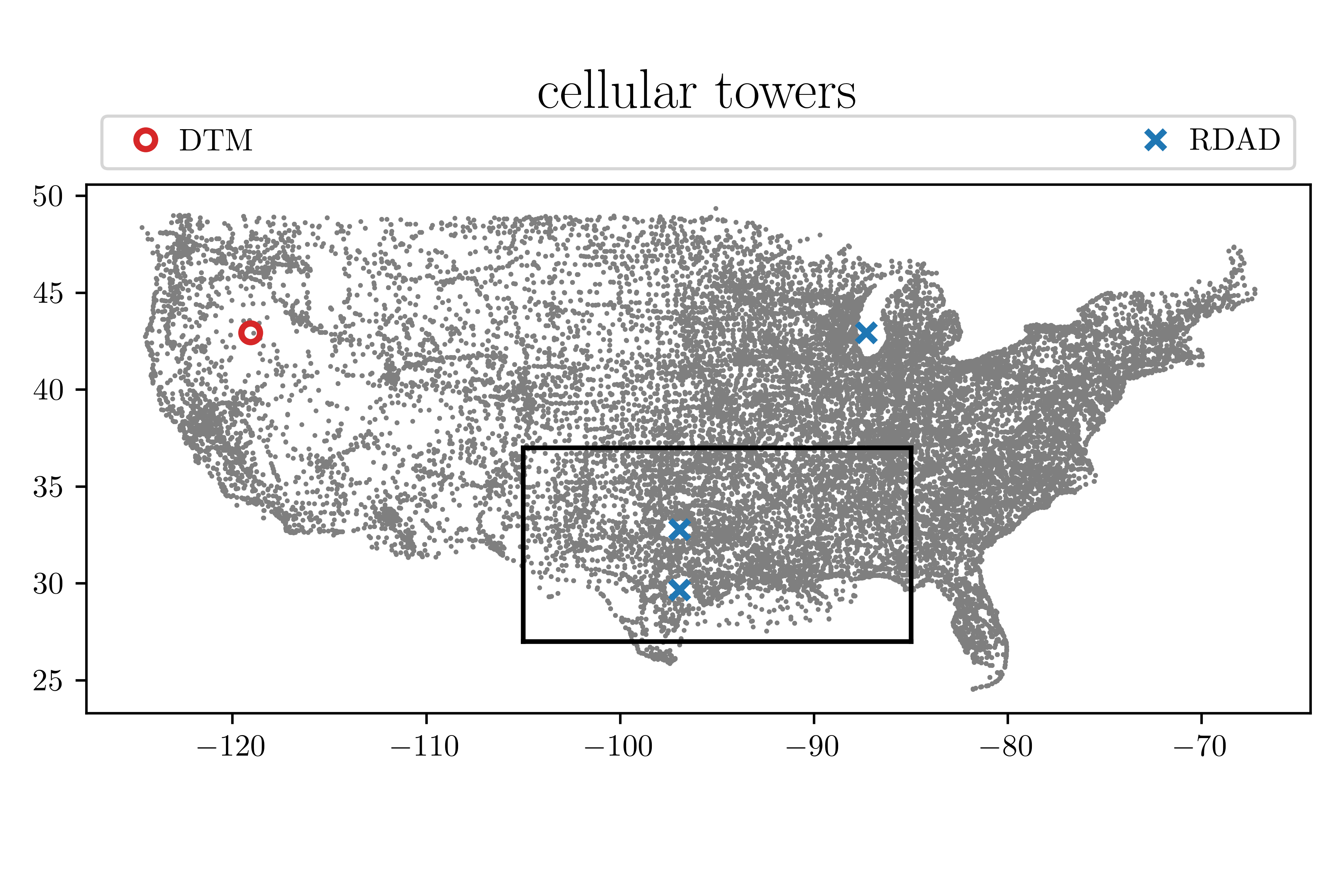
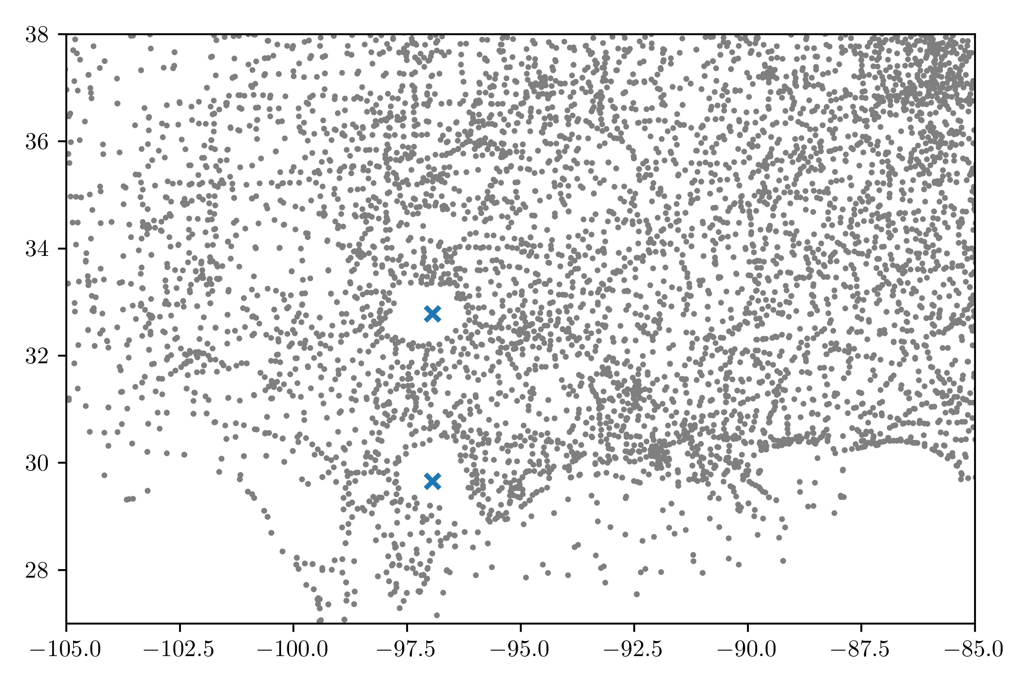
Figure 12: Sample points of the cellular tower dataset (grey dots) and significant loops under subsample bootstrapping for different filtrations (red hollow circles and blue crosses). The black rectangle, which contains two holes detected by RDAD, is blown up and shown on the right subplot.

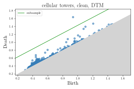
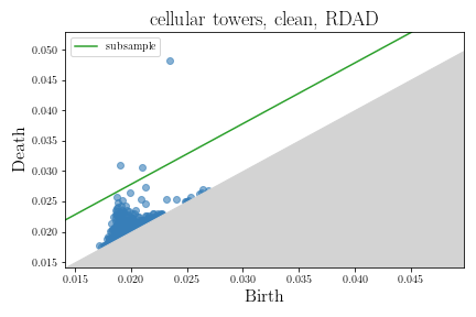
Figure 13: Dimension-1 persistence diagrams of different filtration functions for the cellular tower dataset with confidence bands constructed by subsample bootstrapping.

We also apply our method to real data. The distance-to-measure filtration and the RDAD filtration are applied to an open dataset HIFLD21_cellurlar_towers of cellular tower locations recorded by the Federal Communications Commission (FCC). The two filtrations reveal uninhabited regions in the United States and regions of missing data. As expected, the regions found by the distance-to-measure filtration are large while the small ones are detected only by the RDAD filtration. Details of the dataset and our preprocessing method are summarized in Appendix B.

The scatter plot of the cell towers is shown in Figure 12, followed by the persistence diagrams of the two filtrations in Figure 13. Even without the aid of the confidence bands, one point is conspicuously far away from the diagonal in the persistence diagram of each filtration. The RDAD filtration picks up 2 more significant loops.

The two filtrations pick up completely different homology classes. The class picked up by the distance-to-measure filtration is near Steens Mountain Wilderness in Oregan. The 3 classes picked up by the RDAD filtration are Lake Michigan; Dallas, Texas; and the Texan region surrounded by Houston, Austin and San Antonio. The last two regions have considerable population, and the sparsity of cellular towers there is likely due to the dataset’s incompleteness.

The homology class picked up by the distance-to-measure filtration is a large sparsely populated area with few cellular towers if any. Those picked up by the RDAD filtration are comparatively smaller regions with an abrupt drop in density. The distance-to-measure filtration fails to pick up the smaller homology classes. Even Lake Michigan is too small because of its narrowness. The RDAD filtration cannot detect the large sparsely populated regions because the drop in density there is not sharp enough – nearby regions have very low density anyway.

7 Discussion

While the proposed filtration does prolong the persistences of homology classes of high-density regions in a robust manner, a range of practical, theoretical, statistical and computational issues warrant further investigation.

In practice, while the proposed filtration is designed to handle data with non-uniform density, and can detect well-separated features in a scale-invariant manner, certain large low-density region may cause difficulties.

The effects of the parameters $k_{\text{DTM}}$ and $k_{\text{den}}$ need to be studied in greater detail. For $k_{\text{den}}$, one may use cross-validation to choose a reasonable $k_{\text{den}}$. The effect of different choices of $k_{\text{DTM}}$ is much less understood. In particular, cross-validation does not directly apply because topological signals are inherently global in nature.

Statistically, a theoretical foundation of the bootstrapping method remains to be developed. This is challenging even in the case of the simpler distance-to-measure filtration.

Computationally, in order to obtain a reasonable level of precision, the calculations above are done on a grid, at the cost of restricting the ambient dimension. Computation of the associated Rips complex is likely more feasible.

8 Conclusion

The novel Robust Density-Aware Distance filtration is proposed in the present work for studying data with a non-uniform density. It is designed to make small holes of high-density regions more prominent. It is scale-invariant, and the persistences of homology classes in the proposed filtration depend on the shapes rather than the sizes of the features. Robustness against noise is enhanced through the incorporation of the idea of distance-to-measure. A bootstrapping method is proposed to gauge the significance of a topological feature. The properties of the proposed filtration have been established both theoretically and empirically with artificial and real datasets.

Acknowledgements

The authors would like to thank Andrew Thomas and Jason Manning for insightful conversations.

This research was conducted with support from the Cornell University Center for Advanced Computing, which receives funding from Cornell University, the National Science Foundation, and members of its Partner Program.

All topological computations were done with Gudhi gudhi_CubicalComplex . Nearest-neighbor computations were done with scikit-learn scikit-learn . Numerical computations were done with Numpy numpy , Scipy scipy and Pandas pandas_software ; pandas_article . Codes were compiled with Numba lam15_numba . Graphs were generated with Matplotlib matplotlib .

Funding

Chunyin Siu was supported by Croucher Scholarship for Doctoral Studies. Gennady Samorodnitsky was supported by the NSF grant DMS-2015242 and AFOSR grant FA9550-22-1-0091. Christina Lee Yu was supported by an Intel Rising Stars Award and NSF grants CCF-1948256 and CNS-1955997.

The authors have no relevant financial or non-financial interests to disclose.

Appendix A Proofs

We first establish the main results in Sections 4.1, 4.2 and 4.3 assuming the results from Section 4.4. The latter results are proven in Section A.4. Lemmas will be needed along the way. Unless they are used repeatedly, they will be introduced and proven after they are first used.

A.1 Proofs of Theorem 1 and its Corollaries

We first prove the theorem.

Proof: [Proof of Theorem 1] Suppose first that $x\in\Omega_{i}$ for some $i$. In this case, the lower bound is trivial. Since $P(B(x,\rho_{m}))\geq m$, there exists a mass-$m$ measure $\nu_{x}$ subordinate to $P$ (in the sense defined in Lemma 8) whose support lies in $B(x,\rho_{m})$. By the variational characterization of RDAD (Lemma 8),

$$RDAD(x) \leq\sqrt{\frac{1}{m}\int[f(\xi)^{1/D}d(\xi,x)]^{2}d\nu_{x}(\xi)}\leq\|f\|_{\infty}^{1/D}\rho_{m}=O(\rho_{m}).$$

This gives the upper bound in the theorem.

Let now $y\in\mathbb{R}^{D}\setminus\cup\Omega_{i}$, and for each $i$, let $x_{i}$ be the point nearest to $y$ in $\Omega_{i}$. Since $x_{i}\in\partial\Omega_{i}$, $f(x_{i})=t_{i}$ by assumption.

We first show the upper bound. Again, for each $i$, let $\nu_{i}$ be a mass-$m$ measure subordinate to $P$ whose support lies in $B(x_{i},\rho_{m})\cap f^{-1}[0,at_{i}]$. Then

$$RDAD(y) \leq\sqrt{\frac{1}{m}\int[f(\xi)^{1/D}d(\xi,x)]^{2}d\nu_{i}(\xi)}$$

$$\leq(at_{i})^{1/D}(d(y,x_{i})+\rho_{m})$$

$$=a^{1/D}t_{i}^{1/D}d(y,x_{i})+O(\rho_{m}).$$

Since this is true for every $i$, the upper bound follows.

For the lower bound, let $r$ be such that $F_{y}(r)>m/2$. Since $P(\mathbb{R}^{D}\setminus\cup\Omega_{i})\leq m/2$, the set

$$\{\xi:f(\xi)^{1/D}d(\xi,y)\leq r\}$$

must contain a point $\xi_{0}\in\Omega_{i}$ for some $i$. Then

$$r\geq f(\xi_{0})^{1/D}d(\xi_{0},y)\geq t_{i}^{1/D}d(x_{i},y)=g_{i}(y)\geq g(y).$$

Therefore, for $q>m/2$, since $F_{y}^{(}F_{y}^{-1}(q))\geq q>m/2$, we have $F_{y}^{-1}(q)\geq g(y)$. Hence

$$RDAD(y)\geq\sqrt{\frac{1}{m}\int_{m/2}^{m}F_{y}^{-1}(q)^{2}dq}\geq\frac{1}{\sqrt{2}}g(y).$$

Proof: [Proof of Corollary 2]

Under the sublevel filtration of $g_{i}$, the relevant homology class has birth and death times $t_{i}^{1/D}\beta$ and $t_{i}^{1/D}\delta$. By Lemma 11 below, it also has the same birth and death time under $g$.

Let $\tilde{\beta}=(at_{i})^{1/D}\beta+O(\rho_{m})$ and $\tilde{\delta}=\frac{1}{\sqrt{2}}t_{i}^{1/D}\delta$. Theorem 1 implies

$$g^{-1}[0,t_{i}^{1/D}\beta]\subseteq RDAD^{-1}[0,\tilde{\beta}]\subseteq RDAD^{-1}[0,\tilde{\delta}]\subseteq g^{-1}[0,t_{i}^{1/D}\delta],$$

the class’s persistence under RDAD is then at least $\tilde{\delta}-\tilde{\beta}$.

Lemma 11.

The homology persistence module of the sublevel filtration of $g_{i}$ at levels strictly less than $s_{i}$ is a summand of that of $g$.

Proof: We claim that for every $\varepsilon>0$, on $g_{i}^{-1}[0,s_{i}-\varepsilon]$, $g_{j}>s_{i}>g_{i}$ for every $j\neq i$. Assuming this claim, $g_{i}^{-1}[0,s_{i}-\varepsilon]$ is then a component of $g^{-1}[0,s_{i}-\varepsilon]$, and on this component, $g_{i}$ and $g$ coincide. The lemma then follows.

We now establish the claim. If $g_{i}(x)<s_{i}$, then for every $j\neq i$,

$$t_{i}^{1/D}d(x,\Omega_{i})<s_{i}\leq\frac{d(\Omega_{i},\Omega_{j})}{t_{i}^{-1/D}+t_{j}^{-1/D}},$$

and hence

$$g_{j}(x) =t_{j}^{1/D}d(x,\Omega_{j})$$

$$\geq t_{j}^{1/D}(d(\Omega_{i},\Omega_{j})-d(x,\Omega_{i}))$$

$$\geq t_{j}^{1/D}[(t_{i}^{-1/D}+t_{j}^{-1/D})s_{i}-d(x,\Omega_{i})]$$

$$=s_{i}+t_{j}^{1/D}t_{i}^{-1/D}(s_{i}-t_{i}^{1/D}d(x,\Omega_{i}))$$

$$>s_{i}.$$

The claim then follows.

Since Corollary 3 follows directly from applying Alexander duality to Corollary 2, we omit the proof.

A.2 Proof of Proposition 4

Fix $x$ and let $\tilde{x}=ax+b$. Let $\tilde{P}$ be the measure induced by $\tilde{f}$ and $\tilde{F}_{\tilde{x}}(r)=\tilde{P}[\tilde{f}(\tilde{X})^{1/D}d(\tilde{X},\tilde{x})<r]$.

It suffices to show $\tilde{F}_{\tilde{x}}(r)=F_{x}(r)$ for every $r$.

Let $E_{x}=\{y:f(y)^{1/D}d(y,x)\leq r\}$ and $\tilde{E}_{\tilde{x}}=\{\tilde{y}:\tilde{f}(\tilde{y})^{1/D}d(\tilde{y},\tilde{x})\leq r\}$. Then it can be readily verified that $\tilde{E}_{\tilde{x}}=aE_{x}+b=\{ay+b:y\in E_{x}\}$. Then change of variable formula implies

$$\tilde{F}_{\tilde{x}}(r)=\int_{\tilde{E}_{\tilde{x}}}\tilde{f}(\tilde{y})d\tilde{y}=\int_{E_{x}}f(y)dy=F_{x}(r),$$

from which the equality of the two functions follows.

The equality of the persistence diagrams is now apparent, because the sublevel sets of the two filtrations are scaled and translated versions of each other, and hence share the same topological features.

For the empirical version, the claim is clear because the scaling multiplies both numerator and denominator of $d(x,X_{(i)})/d_{(i)}$ by the same factor, and the translation affects neither of them. The equality of persistence diagrams is analogous to the population case.

A.3 Proofs of Theorem 5 and its Corollary

We first establish some lemmas which will be used throughout the proof of Theorem 5.

The first lemma is a corollary of Hölder’s inequality, and we still call it Hölder’s inequality.

Lemma 12 (Hölder’s Inequality).

Let $\mu$ and $P$ be measures on $X$. Suppose $\mu$ is subordinate to $P$ (in the sense stated in Lemma 8). Then for $p,q,r\in[1,\infty]$ satisfying $\frac{1}{r}=\frac{1}{p}+\frac{1}{q}$,

$$\|\varphi\|_{L^{r}(\mu)}\leq\mu(X)^{1/q}\|\varphi\|_{L^{p}(P)}.$$

Proof: Since $\mu$ is subordinate to $P$, its Radon-Nikodym derivative $\frac{\partial\mu}{\partial P}$ is bounded above by $1$. Since $q/r=q/p+1\geq 1$, $\left(\frac{\partial\mu}{\partial P}\right)^{q/r}\leq\frac{\partial\mu}{\partial P}$. Hölder’s inequality implies

$$\|\varphi\|_{L^{r}(\mu)}=\left\|\varphi\left(\frac{\partial\mu}{\partial P}\right)^{1/r}\right\|_{L^{r}(P)}\leq\|\varphi\|_{L^{p}(P)}\left\|\left(\frac{\partial\mu}{\partial P}\right)^{1/r}\right\|_{L^{q}(P)},$$

and

$$\left\|\left(\frac{\partial\mu}{\partial P}\right)^{1/r}\right\|_{L^{q}(P)}=\left[\int\left(\frac{\partial\mu}{\partial P}\right)^{q/r}dP\right]^{1/q}\leq\left(\int\frac{\partial\mu}{\partial P}dP\right)^{1/q}=\mu(X)^{1/q}.$$

The result then follows.

We will also need the following estimate repeatedly.

Lemma 13 (Estimate on the Distance from a Compact Set).

Let $1\leq p<\infty$. Let $K$ be a compact set in $\mathbb{R}^{D}$ and $x_{0}\in K$. Let $\rho(x)=d(x,x_{0})=\lvert x-x_{0}\rvert$. For any probability measure $P$ with a finite $p^{th}$ moment, $\|\rho\|_{L^{p}(P)}$ has an upper bound that depends only on $p,K$ and the $p^{th}$ moment of $P$ (but not on $x_{0}$).

Proof:

$$\|\rho\|_{L^{p}(P)}=\left(\int\lvert{x-x_{0}}\rvert^{p}dP\right)^{1/p}\leq\lvert{x_{0}}\rvert+\left(\int\lvert{x}\rvert^{p}dP\right)^{1/p}\leq\max_{x^{\prime}\in K}\lvert{x^{\prime}}\rvert+\left(\int\lvert{x}\rvert^{p}dP\right)^{1/p}.$$

We will need other lemmas, but since they will be used only once, we establish them after proving the theorem.

Proof: [Proof of Theorem 5]

Let $P$ and $\tilde{P}$ be the measures induced by $f$ and $\tilde{f}$ on $\mathbb{R}^{D}$.

Fix $x_{0}\in K$ and let $\rho(x)=d(x,x_{0})=\lvert x-x_{0}\rvert$. Let $s=(2^{-1}-r^{-1})^{-1}$.

By the variational characterization of RDAD (Lemma 8), let $\nu^{*}$ be a mass-$m$ measure subordinate to $P$ such that

$$\sqrt{m}RDAD(x_{0}\mathchar 24635\relax\;f,m)=\|f^{1/D}\rho\|_{L^{2}(\nu^{*})}.$$

Let $\Pi$ be an optimal coupling between $P$ and $\tilde{P}$ such that

$$W_{p}(f,\tilde{f})=\|\lvert x-y\rvert\|_{L^{p}(\Pi)}.$$

Let $\tilde{\nu}$ and $\pi$ be subordinate to $\tilde{P}$ and $\Pi$ respectively such that $\pi$ is a coupling between $\nu^{*}$ and $\tilde{\nu}$. They exist by Lemma 14 below.

Again, by the variational characterization of RDAD (Lemma 8) and triangle inequality,

$$\sqrt{m}RDAD(x_{0}\mathchar 24635\relax\;\tilde{f},m)$$

$$\leq\|\tilde{f}^{1/D}\rho\|_{L^{2}(\tilde{\nu})}$$

$$\leq\|f^{1/D}\rho\|_{L^{2}(\nu^{*})}+\left\lvert\|f^{1/D}\rho\|_{L^{2}(\nu^{*})}-\|f^{1/D}\rho\|_{L^{2}(\tilde{\nu})}\right\rvert+\|(\tilde{f}^{1/D}-f^{1/D})\rho\|_{L^{2}(\tilde{\nu})}$$

$$=\sqrt{m}RDAD(x_{0}\mathchar 24635\relax\;f,m)+\left\lvert\|f^{1/D}\rho\|_{L^{2}(\nu^{*})}-\|f^{1/D}\rho\|_{L^{2}(\tilde{\nu})}\right\rvert+\|(\tilde{f}^{1/D}-f^{1/D})\rho\|_{L^{2}(\tilde{\nu})}.$$ (13)

We first estimate the first error term $A=\left\lvert\|f^{1/D}\rho\|_{L^{2}(\nu^{*})}-\|f^{1/D}\rho\|_{L^{2}(\tilde{\nu})}\right\rvert$. Since $\pi$ is a coupling between $\nu^{*}$ and $\tilde{\nu}$, we have

$$\left\lvert\|f^{1/D}\rho\|_{L^{2}(\nu^{*})}-\|f^{1/D}\rho\|_{L^{2}(\tilde{\nu})}\right\rvert =\left\lvert\|(f^{1/D}\rho)(x)\|_{L^{2}(\pi)}-\|(f^{1/D}\rho)(y)\|_{L^{2}(\pi)}\right\rvert$$

$$\leq\|(f^{1/D}\rho)(x)-(f^{1/D}\rho)(y)\|_{L^{2}(\pi)}.$$

Since $\rho$ and $f^{1/D}$ are Lipschitz and $f$ is bounded,

$$\lvert(f^{1/D}\rho)(x)-(f^{1/D}\rho)(y)\rvert\leq\|f\|_{\infty}^{1/D}\lvert x-y\rvert+\text{Lip}(f^{1/D})\rho(x)\lvert x-y\rvert=O((1+\rho(x))\lvert x-y\rvert).$$

Let $u=(r^{-1}-p^{-1})^{-1}$. Recallng the definition of $s$ at the beginning of the proof, we have $2^{-1}=p^{-1}+u^{-1}+s^{-1}$, and hence Hölder’s inequality gives

$$\|(1+\rho(x))\lvert x-y\rvert\|_{L^{2}(\pi)} \leq m^{1/s}\|1+\rho(x)\|_{L^{u}(\Pi)}\|\lvert x-y\rvert\|_{L^{p}(\Pi)}$$

$$=m^{1/s}\|1+\rho\|_{L^{u}(P)}W_{p}(f,\tilde{f}).$$

By Lemma 13, the central factor of the last line is bounded. Therefore,

$$A=O(m^{1/s}W_{p}(f,\tilde{f})).$$

For the second error term

$$B=\|(\tilde{f}^{1/D}-f^{1/D})\rho\|_{L^{2}(\tilde{\nu})}$$

in Equation 13, Hölder’s inequality and Lemma 15 below (applied to $\mu=\tilde{P}$, $\varphi=\tilde{f}$, $\psi=f$, $\theta=\rho$, $p=\infty$) gives

$$B\leq m^{1/s}\|\tilde{f}^{1/D}-f^{1/D}\rho\|_{L^{2}(\tilde{P})}=O(m^{1/s}\|f-\tilde{f}\|_{\infty}^{\frac{D+r}{(D+1)(r+1)}}).$$

Combining the estimates of $A$ and $B$, one side of the bound then follows. The other side is analogous, but not completely symmetric, because $\tilde{f}^{1/D}$ is not assumed to be Lipschitz. We modify the argument above as follows.

Again, let $\sqrt{m}RDAD(x_{0}\mathchar 24635\relax\;\tilde{f})=\|\tilde{f}^{1/D}\rho\|_{L^{2}(\tilde{\nu}^{*})}$. Let $\nu$ and $\tilde{\pi}$ be subordinate to $P$ and $\Pi$ such that $\tilde{\pi}$ is a coupling between $\nu$ to $\tilde{\nu}^{*}$. Then

$$\sqrt{m}RDAD(x_{0}\mathchar 24635\relax\;f)$$

$$\leq\|f^{1/D}\rho\|_{L^{2}(\nu)}$$

$$\leq\|\tilde{f}^{1/D}\rho\|_{L^{2}(\tilde{\nu}^{*})}+\|(\tilde{f}^{1/D}-f^{1/D})\rho\|_{L^{2}(\tilde{\nu}^{*})}+\left\lvert\|f^{1/D}\rho\|_{L^{2}(\tilde{\nu}^{*})}-\|f^{1/D}\rho\|_{L^{2}(\nu)}\right\rvert$$

$$=\sqrt{m}RDAD(x_{0}\mathchar 24635\relax\;\tilde{f})+\|(\tilde{f}^{1/D}-f^{1/D})\rho\|_{L^{2}(\tilde{\nu}^{*})}+\left\lvert\|f^{1/D}\rho\|_{L^{2}(\tilde{\nu}^{*})}-\|f^{1/D}\rho\|_{L^{2}(\nu)}\right\rvert.$$

Since $\tilde{f}$ only appears in the last line in the difference $\tilde{f}^{1/D}-f^{1/D}$, the analysis of these error terms are now completely analogous to that of $A$ and $B$. The proof then follows.

Lemma 14.

Let $P$, $\tilde{P}$ and $\mu$ be measures on a common measurable space, and $\pi$ be a coupling between $P$ and $\tilde{P}$. If $\mu$ is subordinate to $P$ (in the sense defined in Lemma 8), then there exist measures $\tilde{\mu},\tilde{\pi}$ subordinate to $\tilde{P}$ and $\pi$ respectively such that $\tilde{\mu}$ has the same mass as $\mu$ and $\tilde{\pi}$ is a coupling between $\mu$ and $\tilde{\mu}$.

Proof: Since $\mu$ is subordinate to $P$, its Radon-Nikodym derivative $\frac{\partial\mu}{\partial P}$ is bounded above by $1$. Let $d\tilde{\pi}(x,y)=\frac{\partial\mu}{\partial P}(x)d\pi(x,y)$. Then $\tilde{\pi}$ is subordinate to $\pi$; and its $y$-marginal, which we call $\tilde{\mu}$, is subordinate to $\tilde{P}$ and has the same mass as $\mu$.

Lemma 15.

Let $\varphi$ be a bounded moderately tailed density on $\mathbb{R}^{D}$ with parameters $C,\alpha$, where $\alpha\geq D^{2}-D$. Let $\mu$ be the measure induced by $\varphi$ on $\mathbb{R}^{D}$. Let $\psi$ and $\theta$ be measurable functions on $\mathbb{R}^{D}$. Suppose $\psi$ is bounded and nonnegative, and $\theta\in L^{u}(\mu)$ for every $1\leq u<\infty$. Then for $1<r<p\leq\infty$, if $\|\varphi-\psi\|_{L^{p}(\mu)}\leq 1$, then

$$\|(\varphi^{1/D}-\psi^{1/D})\theta\|_{L^{r}(\mu)}=O(\|\varphi-\psi\|_{L^{p}(\mu)}^{\frac{D+r}{(D+1)(r+1)}}),$$

where the big-Oh constant depends only on $\|\varphi\|_{\infty},\|\psi\|_{\infty},p,r,D,C$ and the $L^{u}(\mu)$ norms of $\theta$, where $u$ ranges over $[r,\infty)$.

Proof:

The claim is trivial for $D=1$. Below we assume $D>1$.

Let $0<\eta\leq 1$. We will choose its value later. Note that the following sets cover the whole space:

$$E=\{\varphi>\eta\},\quad F=\{\lvert\varphi-\psi\rvert>\eta^{1-1/D}\},\quad G=\{\varphi\leq\eta,\psi\leq 2\eta^{1-1/D}\}.$$

We estimate the $L^{r}$-norm of $(\varphi^{1/D}-\psi^{1/D})\theta$ on each of the sets above. Let $u=(r^{-1}-p^{-1})^{-1}\geq r$.

For $E$, Hölder’s inequality and the elementary inequality $\lvert a^{1/D}-b^{1/D}\rvert\leq\frac{\lvert a-b\rvert}{a^{1-1/D}}$ give

$$\|(\varphi^{1/D}-\psi^{1/D})\theta\mathbf{1}_{E}\|_{r} \leq\|\theta\|_{u}\|(\varphi^{1/D}-\psi^{1/D})\mathbf{1}_{E}\|_{p}$$

$$\leq\frac{1}{\eta^{1-1/D}}\|\theta\|_{u}\|\varphi-\psi\|_{p}$$

For $F$, Hölder’s inequality and Markov’s inequality imply

$$\|(\varphi^{1/D}-\psi^{1/D})\theta\mathbf{1}_{F}\|_{r} \leq(\|\varphi\|_{\infty}^{1/D}+\|\psi\|_{\infty}^{1/D})\|\theta\|_{u}\|\mathbf{1}_{F}\|_{p}$$

$$\leq(\|\varphi\|_{\infty}^{1/D}+\|\psi\|_{\infty}^{1/D})\|\theta\|_{u}\left(\frac{1}{\eta^{1-1/D}}\|\varphi-\psi\|_{p}\right)$$

For $G$, let $q\in(r,\infty)$, whose value will be chosen later, and let $v=(r^{-1}-q^{-1})^{-1}\geq r$. Hölder’s inequality then gives

$$\|(\varphi^{1/D}-\psi^{1/D})\theta\mathbf{1}_{G}\|_{r} \leq(1+2^{1/D})\eta^{(1-1/D)(1/D)}\|\theta\|_{v}\|\mathbf{1}_{\varphi\leq\eta}\|_{q}$$

$$\leq(1+2^{1/D})\eta^{(1-1/D)(1/D)}\|\theta\|_{v}\|(\mu\{\varphi\leq\eta\}^{1/q}).$$

For the last factor,

$$\mu\{\varphi\leq\eta\}=\int_{\varphi\leq\eta}\varphi(x)dx\leq\int_{\begin{subarray}{c}\varphi\leq\eta\\ \lvert x\rvert\leq R\end{subarray}}\varphi(x)dx+\int_{\lvert x\rvert>R}\varphi(x)dx\leq\omega_{D}\eta R^{D}+CR^{-\alpha}.$$

Since $\alpha\geq D^{2}-D$, putting $R=\eta^{-1/D^{2}}$ gives

$$\mu\{\varphi\leq\eta\}^{1/q}=O(\eta^{(1-1/D)(1/q)}),$$

and hence

$$\|(\varphi^{1/D}-\psi^{1/D})\theta\mathbf{1}_{G}\|_{r}=O(\eta^{(1-1/D)(1/D+1/q)}).$$

Summing the three estimates gives

$$\|(\varphi^{1/D}-\psi^{1/D})\theta\|_{r}=O\left(\frac{1}{\eta^{1-1/D}}\|\varphi-\psi\|_{p}+\eta^{(1-1/D)(1/D+1/q)}\right).$$

The lemma then follows by letting

$$\|\varphi-\psi\|_{p}=\eta^{(1-1/D)(1/q+1/D+1)}\quad\text{and}\quad q=\frac{D(Dr+1)}{(D-1)(D+1)}>r.$$

Note that $q$ is finite when $D>1$.

Proof: [Proof of Corollary 6] Let

$$g^{\text{add}}_{\varepsilon}(x) =\frac{1}{\varepsilon^{D}}g^{\text{add}}(x/\varepsilon)$$

$$\tilde{f}(x) =[(1-\delta)(f*g^{\text{add}}_{\varepsilon})+\delta g^{\text{out}}](x)$$

be the densities of $\varepsilon Y^{\text{add}}$ and $\tilde{X}$. Since $X,Y^{\text{add}}$ and $Y^{\text{out}}$ have moderate tails, so does $\tilde{X}$ (with the same $\alpha$ but possibly a different $C$). Similarly, all moments of $\tilde{X}$ are finite.

Therefore it suffices to let $p=r+1$ and show

$$\|f-\tilde{f}\|_{\infty} =O(\varepsilon+\delta).$$

$$W_{p}(f,\tilde{f}) =O(\varepsilon+\delta^{1/p})$$

We first estimate $\|f-\tilde{f}\|_{\infty}$. For each $x\in\mathbb{R}^{D}$,

$$\lvert\tilde{f}(x)-f(x)\rvert$$

$$\leq(1-\delta)\int g^{\text{add}}_{\varepsilon}(x-y)\lvert f(y)-f(x)\rvert dy+\delta\lvert g^{\text{out}}-f\rvert$$

$$\leq\int\lvert x-y\rvert g^{\text{add}}_{\varepsilon}(x-y)\frac{\lvert f(y)-f(x)\rvert}{\lvert x-y\rvert}dy+O(\delta) f,g^{\text{out}}$$ ( bounded)

$$=O(\int\lvert x-y\rvert g^{\text{add}}_{\varepsilon}(x-y)dy)+O(\delta) \text{($f$ Lipschitz)}.$$

$f$ is Lipschitz because $f^{1/D}$ is and $x\mapsto x^{D}$ is Lipschitz on $[0,\|f\|_{\infty}^{1/D}]$. For the first term,

$$\int\lvert x-y\rvert g^{\text{add}}_{\varepsilon}(x-y)dy=\int\lvert y\rvert g^{\text{add}}_{\varepsilon}(y)dy=E\lvert\varepsilon Y^{\text{add}}\rvert=O(\varepsilon).$$

The first estimate then follows.

For $W_{p}(f,\tilde{f})$, let $\Pi^{\text{out}}$ be a coupling between $f(x)dx$ and $g^{\text{out}}(y)dy$. Then

$$\|\lvert x-y\rvert\|_{L^{p}(\Pi^{\text{out}})}=O(1),$$

because all moments of $f$ and $g^{\text{out}}$ are finite, the two densities have finite Wasserstein distances from the dirac delta measure at $0$.

Consider the following coupling between $P$ and $\tilde{P}$:

$$d\Pi(x,y)=(1-\delta)g^{\text{add}}_{\varepsilon}(y-x)f(x)dxdy+\delta d\Pi^{\text{out}}(x,y).$$

Then

$$W_{p}(f,\tilde{f})^{p} \leq\|\lvert x-y\rvert\|_{L^{p}(\Pi)}^{p}$$

$$=\int(1-\delta)\lvert x-y\rvert^{p}g_{\varepsilon}(y-x)f(x)dxdy+\delta\|\lvert x-y\rvert\|_{L^{p}(\Pi^{\text{out}})}^{p}$$

$$\leq\int[\lvert z\rvert^{p}g_{\varepsilon}(z)f(x)dxdz+O(\delta) (z=y-x)$$

$$=E[\lvert\varepsilon Y^{\text{add}}\rvert^{p}]+O(\delta)$$

$$=O(\varepsilon^{p}+\delta).$$

The result then follows.

A.4 Proofs of Properties in Section 4.4

In this subsection, we establish properties of RDAD in Section 4.4 in logical order. The results proven in previous sections rely on these properties. Since none of the following proofs depend on those previous results, with the sole exception that Proposition 9 depends on Hölder’s inequality (Lemma 12), which does not depend on any results in this section, our arguments are not circular.

Proof: [Proof of Lemma 8] The argument is similar to that in the proof of Proposition 2.2 of buchet16_DTM_approximation .

Fix $x$ and fix a mass-$m$ measure $\nu$ that is subordinate to $P$. Consider the random variable $Y=f(X)^{1/D}d(X,x)$.

Let $F_{P}^{-1}$ and $F_{\nu}^{-1}$ be the quantile functions of $Y$ under $P$ and $\nu$ respectively. Then $m\cdot RDAD(x)^{2}=\int_{0}^{m}F_{P}^{-1}(q)^{2}dq$.

The change of variable formula gives an analogous expression for $\nu$:

$$\int[f(\xi)^{1/D}d(\xi,x)]^{2}d\nu(\xi)=\int Y^{2}dF_{\nu}=\int_{0}^{m}F_{\nu}^{-1}(t)^{2}dt.$$

Since $\nu$ is suborindate to $P$,

$$F_{P}^{-1}\leq F_{\nu}^{-1},$$ (14)

hence

$$\int[f(\xi)^{1/D}d(\xi,x)]^{2}d\nu(\xi)\geq\int_{0}^{m}F_{P}^{-1}(q)^{2}dq=m\cdot RDAD(x)^{2}.$$

This proves one inequality in the lemma.

To finish the proof, it suffices to find a $\nu$ such that equality holds on $(0,m)$ in Equation 14. Let

$$E_{<} =\{\xi:f(\xi)^{1/D}d(\xi,x)<F^{-1}_{P}(m)\}$$

$$E_{=} =\{\xi:f(\xi)^{1/D}d(\xi,x)=F^{-1}_{P}(m)\}.$$

Define

$$\nu=P\mid E_{<}+(m-P(E_{<}))\frac{P\mid E_{=}}{P(E_{=})}.$$

This $\nu$ has the desired property, because by construction, $F_{P}(y)=F_{\nu}(y)$ for $y<F^{-1}_{P}(m)$, and hence $F_{P}^{-1}(t)=F_{\nu}^{-1}(t)$ for $t<m$. The result then follows.

Proof: [Proofs of Propositions 9 and 7]

We first prove the Lipschitz continuity of RDAD. Then we prove the convergence of RDAD to DAD. Lipschitz continuity of DAD then follows from the locally uniform convergence of RDAD to DAD.

For Lipschitz continuity of RDAD, when $2<p<\infty$, Lemma 8 implies

$$RDAD(x)=\frac{1}{\sqrt{m}}\|f(\cdot)^{1/D}d(\cdot,x)\|_{L^{2}(\nu_{x})}$$

for some mass-$m$ measure $\nu_{x}$. Now, letting $q=(2^{-1}-p^{-1})^{-1}$

$$RDAD(y) \leq\frac{1}{\sqrt{m}}\|f(\cdot)^{1/D}d(\cdot,y)\|_{L^{2}(\nu_{x})}$$

$$\leq\frac{1}{\sqrt{m}}\|f(\cdot)^{1/D}d(x,y)+f(\cdot)^{1/D}d(\cdot,x)\|_{L^{2}(\nu_{x})}$$

$$\leq\frac{1}{\sqrt{m}}\|f(\cdot)^{1/D}d(x,y)\|_{L^{2}(\nu_{x})}+\frac{1}{\sqrt{m}}\|f(\cdot)^{1/D}d(\cdot,x)\|_{L^{2}(\nu_{x})}$$

$$=\frac{1}{\sqrt{m}}\|f(\cdot)^{1/D}\|_{L^{2}(\nu_{x})}d(x,y)+RDAD(x)$$

$$\leq\frac{1}{\sqrt{m}}m^{1/q}\|f^{1/D}\|_{L^{p}(P)}d(x,y)+RDAD(x).$$

$$=\left[\frac{1}{m^{1/p}}\left(\int f(\xi)^{1+p/D}d\xi\right)^{1/p}\right]d(x,y)+RDAD(x).$$

Lipschitz continuity of RDAD then follows by interchanging $x$ and $y$.

When $f$ is bounded, the above argument follows through if we take $p=\infty$. The following adaptations are necessary: $1/q$ is now $1/2$, and $\|f^{1/D}\|_{L^{p}(P)}$ in the second last line and the factor in the square bracket in the last line each needs to be replaced by $\|f^{1/D}\|_{\infty}=\|f\|_{\infty}^{1/D}$.

For the convergence of RDAD to DAD, since $RDAD(x)$ is the $L^{2}$ average of $F_{x}^{-1}(q)$ on $[0,m]$ and $F_{x}^{-1}$ is increasing,

$$DAD(x)=\lim_{q\to 0^{+}}F_{x}^{-1}(q)\leq RDAD(x)\leq F_{x}^{-1}(m).$$

For each $x$, the right-hand side converges to $\lim_{q\to 0^{+}}F_{x}^{-1}(q)$ as $m\to 0$ by definition, and the limit is just $DAD(x)$. Pointwise convergence then follows.

For uniform convergence on compact sets under the assumption that $f$ is bounded, Lipscthiz continuity of RDAD implies $\{RDAD(\cdot\mathchar 24635\relax\;f,m)\}_{m\in(0,1]}$ is equicontinuous. By Arzela-Ascoli theorem, pointwise convergence of the family implies uniform convergence on compact sets.

Before proving Proposition 10, we need a lemma, which is the counterpart of Lemma 8 in chazal18_DTM_statistics :

Lemma 16.

Let $f:\mathbb{R}^{D}\to\mathbb{R}$ be a density with bounded support and a finite upper bound. Let $P$ be the probability measure on $\mathbb{R}^{D}$ with density $f$. Let $0<m<1$. Then $F_{x}^{-1}(m)$ is Lipschitz in $x$ on $\mathbb{R}^{D}$, and $(F_{x}^{-1}(m))^{2}$ is Lipschitz in $x$ on every compact set in $\mathbb{R}^{D}$.

Proof: The second claim follows from the first because the square of any Lipschitz function on a compact metric space is always Lipschitz.

To establish the first claim, we have, by definition

$$F_{x}^{-1}(m)=\inf\{t:P\left(f(X)^{1/D}d(x,X)\leq t\right)\geq m\}.$$

Since for any $x^{\prime}$,

$$\{y:f(y)^{1/D}d(x,y)\leq t\}\subseteq\{y:f(y)^{1/D}d(x^{\prime},y)\leq t+\|f\|_{\infty}^{1/D}d(x,x^{\prime})\},$$

whenever

$$P\left(f(X)^{1/D}d(x,X)\leq t\right)\geq m$$

holds, we have

$$P\left(f(X)^{1/D}d(x^{\prime},X)\leq t+\|f\|_{\infty}^{1/D}d(x,x^{\prime})\right)\geq m.$$

Taking infimum over $t$ gives

$$F_{x^{\prime}}^{-1}(m)\leq F_{x}^{-1}(m)+\|f\|_{\infty}^{1/D}d(x,x^{\prime}).$$

Interchanging $x$ and $x^{\prime}$ shows $F_{x}^{-1}(m)$ is Lipschitz in $x$ with Lipschitz constant bounded by $\|f\|_{\infty}^{1/D}$.

We are now in the position to prove Proposition 10.

Proof: [Proofs of Proposition 10] We adapt the proofs of Theorems 5 and 9 of chazal18_DTM_statistics , the former of which is a stepping stone towards proving Theorem 9 therein.

Under the assumption of uniform continuity,

$$\|\hat{f}_{k_{den}}-f\|_{\infty}\to 0$$

almost surely (Theorem 4.2 of biau_devroye_nearest_neigbhor ). Then almost surely,

$$\max_{i}\lvert C_{N,k_{\text{den}},D}1/d_{i}-f(X_{i})^{1/D}\rvert\to 0,$$

hence

$$\sup_{x\in K}\left\lvert\widehat{RDAD}^{2}(x)-\frac{1}{k_{\text{DTM}}}\sum[f(X_{(i)})^{1/D}d(x,X_{(i)})]^{2}\right\lvert=o_{P}(1).$$

The rest of the proof of Proposition 10 then follows by replacing each instance of $F_{x}$ in the proofs of Theorems 5 and 9 of chazal18_DTM_statistics with

$$\mathcal{F}_{x}(t)=P((f(X)^{1/D}d(x,X))^{2}\leq t).$$ (15)

Note that $\mathcal{F}_{x}(t)=F_{x}(\sqrt{t})$, where $F_{x}$ is defined in Equation 8, which is different from the $F_{x}$ in chazal18_DTM_statistics , and this is the origin of the square roots in our statement, which are not present in its counterpart in chazal18_DTM_statistics .

Below, we sketch the main ideas for completeness. We will highlight non-trivial adaptations and refer the readers to chazal18_DTM_statistics for details.

The proof starts with the observation

$$\sqrt{n}(\widehat{RDAD}^{2}(x)-RDAD^{2}(x))=A_{n}(x)+R_{n}(x),$$

where

$$A_{n}(x) =\frac{1}{m}\int_{0}^{\mathcal{F}_{x}^{-1}(m)}\sqrt{n}(\mathcal{F}_{x}(t)-\hat{\mathcal{F}_{x}}(t))dt$$

$$R_{n}(x) =\frac{1}{m}\int_{\mathcal{F}_{x}^{-1}(m)}^{\hat{\mathcal{F}}_{x}^{-1}(m)}\sqrt{n}(m-\hat{\mathcal{F}_{x}}(t))dt,$$

where $\hat{\mathcal{F}_{x}}$ is defined as in Equation 15 with the probability replaced by the empirical measure.

$R_{n}$ can be bounded with the estimate

$$\lvert{R_{n}(x)}\rvert\leq\frac{\sqrt{n}}{m}\lvert{S_{n}(x)}\rvert\lvert{T_{n}(x)}\rvert,$$

where

$$S_{n}(x)=\lvert{\mathcal{F}_{x}^{-1}(m)-\hat{\mathcal{F}}_{x}^{-1}(m)}\rvert,\quad T_{n}(x)=\sup_{t}\lvert{\mathcal{F}_{x}(t)-\hat{\mathcal{F}_{x}}(t)}\rvert.$$

By exactly the same empirical process theory argument as in chazal18_DTM_statistics (with all instances of Lemma 8 in chazal18_DTM_statistics replaced by Lemma 16 here), one can show

$$\sup_{x\in K}\lvert S_{n}(x)\rvert=o_{P}(1).$$

For $T_{n}$, by Vapnik-Chernvonenkis theorem,

$$\sup_{x\in K}\lvert T_{n}(x)\rvert\leq\sup_{\begin{subarray}{c}z\in\mathbb{R}^{D}\\ r>0\end{subarray}}\lvert\hat{P_{n}}(E_{z,r})-P(E_{z,r})\rvert=O(1/\sqrt{n}).$$

The theorem is indeed applicable because the relevant classifying functions for the $E_{z,r}$’s form a subset of a finite-dimensional space, specifically:

$$f(\cdot)^{2/D}d(z,\cdot)^{2}-t\in\text{span}\{f(\cdot)^{2/D}\|\cdot\|^{2},f(\cdot)^{2/D}z_{1},...,f(\cdot)^{2/D}z_{D},f(\cdot)^{2/D},t\}.$$

It remains to show $A_{n}$ converges to a Gaussian process. Let $\nu_{n}=\sqrt{n}(\hat{P}_{n}-P)$. Note that

$$A_{n}=\frac{1}{m}\int f_{x}(y)d\nu_{n}(y),$$

where

$$f_{x}(y)=\max(0,\mathcal{F}_{x}^{-1}(m)-(f(y)\lvert{x-y}\rvert)^{2}),$$

By Donsker’s theorem, it suffices to show $f_{x}$’s form a $P$-Donsker family. By Example 19.7 of vaart98_asymptoticStat , indeed they do:

$$\lvert f_{x}(y)-f_{x^{\prime}}(y)\rvert \leq\lvert\mathcal{F}_{x}^{-1}(m)-\mathcal{F}_{x^{\prime}}^{-1}(m)\rvert+\|x-x^{\prime}\|(\|x\|+\|x^{\prime}\|+2\|y\|)\lvert f(y)\rvert,$$

$$\leq\lvert\mathcal{F}_{x}^{-1}(m)-\mathcal{F}_{x^{\prime}}^{-1}(m)\rvert+\|x-x^{\prime}\|(2\text{diam }K+\text{diam }\text{supp}f)\|f\|_{\infty},$$

where the first term is bounded by a multiple of $\|x-x^{\prime}\|$ because Lemma 16 shows $\mathcal{F}_{x}^{-1}(m)=(F_{x}^{-1}(m))^{2}$ is Lipschitz in $x$.

Finally, the claim on the covariance kernel follows from passing the convariance of $A_{n}$ to the limit.

Appendix B Details of Simulations

We give details on the constructions of our synthetic datasets, and the parameters used in our experiments, in this section. Model parameters are summarized in Table 1. The sample sizes and the density estimation parameters $k_{\text{den}}$, which depends on the sample sizes, are summarized in Table 2.

parameters	values	meaning
$k_{\text{den}}$	$\lceil(\log_{10}N)^{2}\rceil$	density estimated by the $k_{\text{den}}$-nearest neighbor estimator; $N$ is the sample size
$m_{\text{DTM}}$	0.002	amount of mass taken into account by the distance-to-measure setup
$\Delta x$ (two-square)	0.02	grid size at which the filtration functions are evaluated in the two-square experiments
$\Delta x$ (Voronoi)	0.01	grid size at which the filtration functions are evaluated in the Voronoi experiment
$\Delta x$ (cellular towers)	0.260	grid size at which the filtration functions are evaluated in the cellular tower experiment
$B$	100	the number of bootstrap samples
$\alpha$	0.05	Confidence sets are bottleneck metric balls whose radii are $(1-\alpha)$-percentile of the bottleneck distances of the empirical persistence diagram from the diagrams of the bootstrap samples.

Table 1: Model parameters used in the simulations.

datasets	$N$	$k_{\text{den}}$
two-square – David and Goliath	500	8
two-square – all others	5000	14
Voronoi – noisy	10676	17
cellular towers	23389	20

Table 2: Sample sizes ($N$) and density estimation paremeter $k_{\text{den}}$ For different datasets.

For two-square datasets, the precise values used are summarized in Table 3. The inner radius $r$ and outer radius $R$ of a square annulus refer to half of the sidelengths of the inner and outer squares in a square annulus. This is illustrated in Figure 14.

parameters	David & Goliath	other datasets	meanings
$(x_{1},x_{2})$	(0, 4)	(0, 4)	$x$-coordinates of centers of the square annuli
$(y_{1},y_{2})$	(0, 0)	(0, 0)	$y$-coordinates of centers of the square annuli
$(p_{1},p_{2})$	(0.4, 0.6)	(0.5, 0.5)	masses of the square annuli
$(r_{1},r_{2})$	(1, 0.1)	(1, 1/3)	inner radii of the square annuli, see Figure 14
$(R_{1},R_{2})$	(1.1, 0.12)	(1.4, 1.4/3)	outer radii of the square annuli, see Figure 14
$(\sigma_{1},\sigma_{2})$	–	(0.15, 0.05)	standard deviations of the isotropic Gaussian noises on the square annuli
$N_{\text{outliers}}$	–	8	number of outliers

Table 3: Parameters used to generate two-square datasets (in alphabetical order, Greek letters follow Latin ones).

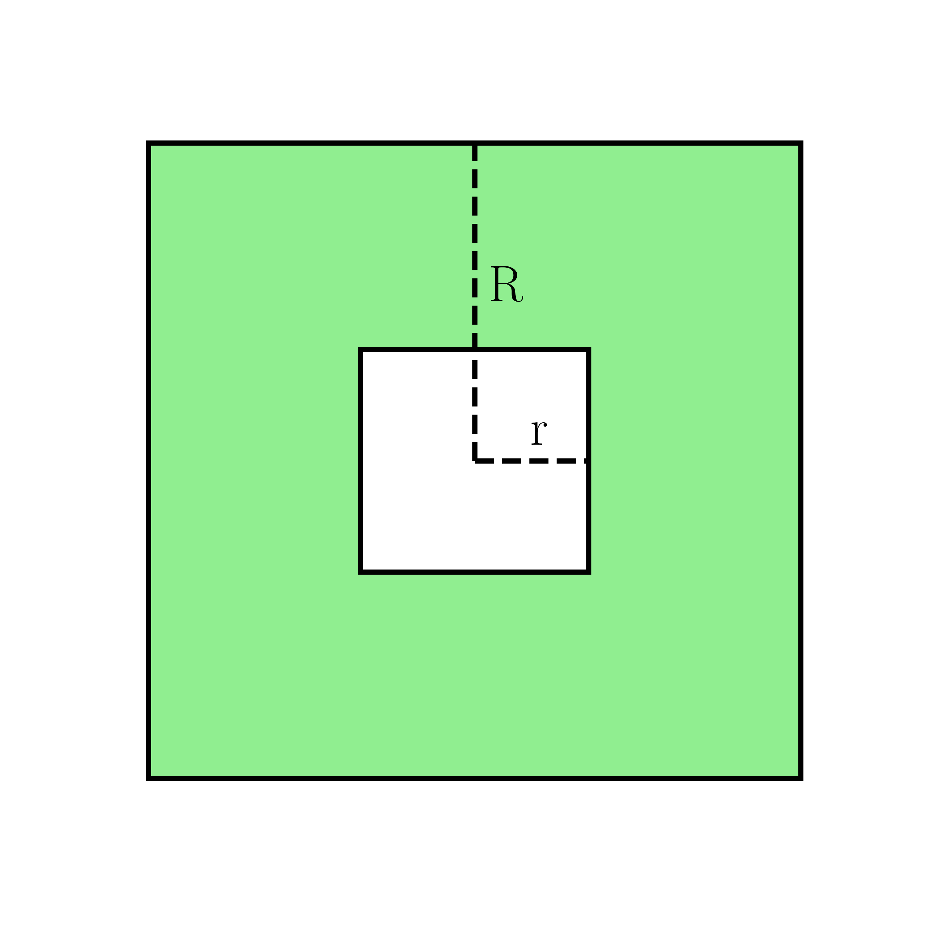
Figure 14: Inner and outer radii of a square annulus

For the Voronoi dataset, we first describe the data generation process. The actual values of parameters used is summarized in Table 4.

Generation of the Voronoi diagram

A fixed number $M^{+}_{\text{cell}}$ of centers of Voronoi cells are sample points on an infinite strip $\mathbb{R}\times[-y_{+},y_{+}]$ so that more points will be near the central vertical line $y=0$. Specifically, the $x$- and $y$-coordinates are sampled independently from a biexponential distribution $\text{Biexp}(\lambda)$ with scale parameter $\lambda$ and a uniform distribution respectively. The Voronoi diagram is then generated from these Voronoi cell centers. Since more points are sampled at the central vertical line, cells near the line are smaller than those on the right.

Generation of a super-sample

We sample $N^{+}$ points from the equal-weight mixture of the uniform measures supported on the boundaries of the cells. Then smaller cells have edges with higher edge density.

Corruption by additive noise

To add noise to the dataset, for each sample point $(x,y)$ on edges of the Voronoi diagram, we perturb it with independent mean-zero isotropic Gaussian noise, whose standard deviation is $\sigma_{0}e^{\lvert x\rvert/\lambda}$, so points near the central vertical line are corrupted by a smaller noise.

Removal of ill-behaving points to obtain the sample

Since cells near the boundary, even if finite, tend to be very elongated, we discard all points outside of a rectangle $R$. This motivates our choice that outliers lie in $R$, because outliers lying outside of $R$ will be discarded. We analyze the dataset formed by the remaining $N$ points. The framing rectangles of the scatter plots as well as plots of significant loops in Section 6.2 are all the rectangle $R$.

parameters	values	meaning
$M_{\text{cell}}$	88	number of Voronoi cells completely contained in the rectangle $R$
$M^{+}_{\text{cell}}$	200	number of cells in the full Voronoi diagram
$N^{+}$	20000	number of sample points in the full Voronoi diagram
$p_{\text{outlier}}$	0.002	proportion of the $N^{+}$ sample points that are replaced by outliers
$R$	–	the rectangle $[-x_{0},x_{0}]\times[-y_{0},y_{0}]$ only on which sample points are passed to topological computation
$x_{0}$	3	maximum absolute value of the $x$-coordinates of sample points that are passed to topological computation
$y_{0}$	1	maximum absolute value of the $y$-coordinates of sample points that are passed to topological computation
$y_{+}$	2	maximum possible absolute values of the $y$-coordinates of Voronoi cell centers
$\lambda$	1	scale parameter of the biexponential distribution, from which the $x$-coordinates of Voronoi cell centers are drawn
$\sigma_{0}$	0.01	scale parameter of the additive Gaussian noise

Table 4: Parameters used to generate Voronoi datasets

For the cellular tower dataset, it is preprocessed as follows. Only towers in the contiguous United States are retained. Incorrectly labelled towers are left as-is, except that one Texas tower, which is erroneously labelled to be in the middle of the Atlantic Ocean, is removed. We treat the longitude and latitude of each of the remaining 23389 towers as the $x$- and $y$-coordinates of a data point.

From the data points, the filtration function values are evaluated on the grid, on the rectangle $[-126,-65.8]\times[23.9,50.0]$, which contains all points. The grid size is $1/100^{th}$ of the shorter side of the rectangle.

References

- \bibcommenthead
- (1) Icke, V., van de Weygaert, R.: The galaxy distribution as a Voronoi foam. QJRAS 32, 85–112 (1991)
- (2) Carlsson, G.: Topology and data. Bulletin of the American Mathematical Society 46, 255–308 (2009)
- (3) Chazal, F., Michel, B.: An introduction to topological data analysis: Fundamental and practical aspects for data scientists. Frontiers in Artificial Intelligence 4 (2021). https://doi.org/10.3389/frai.2021.667963
- (4) Perea, J.A.: Topological time series analysis. AMS Notices 66(5), 686–694 (2019)
- (5) Aktas, M.E., Akbas, E., Fatmaoui, A.E.: Persistence homology of networks: methods and applications. Applied Network Science 4(1), 61 (2019). https://doi.org/10.1007/s41109-019-0179-3
- (6) Buchet, M., Hiraoka, Y., Obayashi, I.: In: Tanaka, I. (ed.) Persistent Homology and Materials Informatics, pp. 75–95. Springer, Singapore (2018). https://doi.org/10.1007/978-981-10-7617-6_5. https://doi.org/10.1007/978-981-10-7617-6_5
- (7) Xu, X., Cisewski-Kehe, J., Green, S.B., Nagai, D.: Finding cosmic voids and filament loops using topological data analysis. Astronomy and Computing 27, 34–52 (2019). https://doi.org/10.1016/j.ascom.2019.02.003
- (8) Salch, A., Regalski, A., Abdallah, H., Suryadevara, R., Catanzaro, M.J., Diwadkar, V.A.: From mathematics to medicine: A practical primer on topological data analysis (tda) and the development of related analytic tools for the functional discovery of latent structure in fmri data. PLOS ONE 16(8), 1–33 (2021). https://doi.org/10.1371/journal.pone.0255859
- (9) Stolz, B.J., Harrington, H.A., Porter, M.A.: Persistent homology of time-dependent functional networks constructed from coupled time series. Chaos: An Interdisciplinary Journal of Nonlinear Science 27(4), 047410 (2017). https://doi.org/10.1063/1.4978997
- (10) Feng, M., Porter, M.A.: Persistent homology of geospatial data: A case study with voting. SIAM Review 63(1), 67–99 (2021). https://doi.org/10.1137/19M1241519
- (11) Jaquette, J., Schweinhart, B.: Fractal dimension estimation with persistent homology: A comparative study. Communications in Nonlinear Science and Numerical Simulation 84, 105163 (2020). https://doi.org/10.1016/j.cnsns.2019.105163
- (12) Bubenik, P., Hull, M., Patel, D., Whittle, B.: Persistent homology detects curvature. Inverse Problems 36(2), 025008 (2020). https://doi.org/10.1088/1361-6420/ab4ac0
- (13) Motta, F.C., Neville, R., Shipman, P.D., Pearson, D.A., Bradley, R.M.: Measures of order for nearly hexagonal lattices. Physica D: Nonlinear Phenomena 380-381, 17–30 (2018). https://doi.org/10.1016/j.physd.2018.05.005
- (14) Xia, K., Wei, G.-W.: Persistent homology analysis of protein structure, flexibility, and folding. International Journal for Numerical Methods in Biomedical Engineering 30(8), 814–844 (2014). https://doi.org/10.1002/cnm.2655
- (15) Aragon-Calvo, M.A., Szalay, A.S.: The hierarchical structure and dynamics of voids. Monthly Notices of the Royal Astronomical Society 428(4), 3409–3424 (2012). https://doi.org/10.1093/mnras/sts281
- (16) Wilding, G., Nevenzeel, K., van de Weygaert, R., Vegter, G., Pranav, P., Jones, B.J.T., Efstathiou, K., Feldbrugge, J.: Persistent homology of the cosmic web – I. Hierarchical topology in CDM cosmologies. Monthly Notices of the Royal Astronomical Society 507(2), 2968–2990 (2021). https://doi.org/10.1093/mnras/stab2326
- (17) Bendich, P., Marron, J.S., Miller, E., Pieloch, A., Skwerer, S.: Persistent homology analysis of brain artery trees. The Annals of Applied Statistics 10(1), 198–218 (2016). https://doi.org/10.1214/15-AOAS886
- (18) Carlsson, G., Zomorodian, A.: The theory of multidimensional persistence. Discrete Comput. Geom., 71–93 (2009)
- (19) Sheehy, D.R.: A multicover nerve for geometric inference. In: CCCG: Canadian Conference in Computational Geometry (2012)
- (20) Blumberg, A.J., Lesnick, M.: Stability of 2-Parameter Persistent Homology (2021)
- (21) Lesnick, M., Wright, M.: Interactive Visualization of 2-D Persistence Modules (2015)
- (22) Moon, C., Giansiracusa, N., Lazar, N.A.: Persistence terrace for topological inference of point cloud data. Journal of Computational and Graphical Statistics 27(3), 576–586 (2018). https://doi.org/10.1080/10618600.2017.1422432
- (23) Berry, T., Sauer, T.: Consistent manifold representation for topological data analysis. Foundations of Data Science 1(1), 1–38 (2019)
- (24) Hickok, A.: A Family of Density-Scaled Filtered Complexes (2022)
- (25) Bell, G., Lawson, A., Martin, J., Rudzinski, J., Smyth, C.: Weighted persistent homology. Involve 12(5), 823–837 (2019). https://doi.org/10.2140/involve.2019.12.823
- (26) Chazal, F., Cohen-Steiner, D., Mérigot, Q.: Geometric inference for probability measures. Found Comput Math 11, 733–751 (2011). https://doi.org/10.1007/s10208-011-9098-0
- (27) Buchet, M., Chazal, F., Oudot, S.Y., Sheehy, D.R.: Efficient and robust persistent homology for measures. Computational Geometry 58, 70–96 (2016). https://doi.org/10.1016/j.comgeo.2016.07.001
- (28) Chazal, F., Fasy, B., Lecci, F., Michel, B., Rinaldo, A., Wasserman, L.: Robust topological inference: Distance to a measure and kernel distance. Journal of Machine Learning Research 18, 1–40 (2018)
- (29) Anai, H., Chazal, F., Glisse, M., Ike, Y., Inakoshi, H., Tinarrage, R., Umeda, Y.: DTM-Based Filtrations. In: Barequet, G., Wang, Y. (eds.) 35th International Symposium on Computational Geometry (SoCG 2019). Leibniz International Proceedings in Informatics (LIPIcs), vol. 129, pp. 58–15815. Schloss Dagstuhl–Leibniz-Zentrum fuer Informatik, Dagstuhl, Germany (2019). https://doi.org/10.4230/LIPIcs.SoCG.2019.58. http://drops.dagstuhl.de/opus/volltexte/2019/10462
- (30) Edelsbrunner, H., Harer, J.: Computational Topology: An Introduction. Applied Mathematics. American Mathematical Society, Providence, RI (2010). https://www.ams.org/books/mbk/069/
- (31) Otter, N., Porter, M.A., Tillmann, U., Grindrod, P., Harrington, H.A.: A roadmap for the computation of persistent homology. EPJ Data Science 6(1), 17 (2017). https://doi.org/10.1140/epjds/s13688-017-0109-5
- (32) Fasy, B.T., Lecci, F., Rinaldo, A., Wasserman, L., Balakrishnan, S., Singh, A.: Confidence sets for persistence diagrams. The Annals of Statistics 42(6), 2301–2339 (2014)
- (33) Silverman, B.W.: Density Estimation for Statistics and Data Analysis, 1st edn. Chapman & Hall/ CRC, Boca Raton, FL (2003)
- (34) Biau, G., Devroye, L.: Lectures on the Nearest Neighbor Method, 1st edn. Springer, Cham, Switzerland (2015). https://link.springer.com/book/10.1007/978-3-319-25388-6
- (35) Dlotko, P.: Cubical complex. In: GUDHI User and Reference Manual, 3.4.1 edn. GUDHI Editorial Board, Saclay, France (2021). https://gudhi.inria.fr/doc/3.4.1/group__cubical__complex.html
- (36) Pranav, P., Edelsbrunner, H., van de Weygaert, R., Vegter, G., Kerber, M., Jones, B.J.T., Wintraecken, M.: The topology of the cosmic web in terms of persistent Betti numbers. Monthly Notices of the Royal Astronomical Society 465(4), 4281–4310 (2016). https://doi.org/10.1093/mnras/stw2862
- (37) HIFLD: Cellular Towers. https://hifld-geoplatform.opendata.arcgis.com/datasets/cellular-towers/explore?location=26.819085%2C-53.792376%2C2.76&showTable=true
- (38) Pedregosa, F., Varoquaux, G., Gramfort, A., Michel, V., Thirion, B., Grisel, O., Blondel, M., Prettenhofer, P., Weiss, R., Dubourg, V., Vanderplas, J., Passos, A., Cournapeau, D., Brucher, M., Perrot, M., Duchesnay, E.: Scikit-learn: Machine learning in Python. Journal of Machine Learning Research 12, 2825–2830 (2011)
- (39) Harris, C.R., Millman, K.J., van der Walt, S.J., Gommers, R., Virtanen, P., Cournapeau, D., Wieser, E., Taylor, J., Berg, S., Smith, N.J., Kern, R., Picus, M., Hoyer, S., van Kerkwijk, M.H., Brett, M., Haldane, A., del Río, J.F., Wiebe, M., Peterson, P., Gérard-Marchant, P., Sheppard, K., Reddy, T., Weckesser, W., Abbasi, H., Gohlke, C., Oliphant, T.E.: Array programming with NumPy. Nature 585(7825), 357–362 (2020). https://doi.org/10.1038/s41586-020-2649-2
- (40) Virtanen, P., Gommers, R., Oliphant, T.E., Haberland, M., Reddy, T., Cournapeau, D., Burovski, E., Peterson, P., Weckesser, W., Bright, J., van der Walt, S.J., Brett, M., Wilson, J., Millman, K.J., Mayorov, N., Nelson, A.R.J., Jones, E., Kern, R., Larson, E., Carey, C.J., Polat, İ., Feng, Y., Moore, E.W., VanderPlas, J., Laxalde, D., Perktold, J., Cimrman, R., Henriksen, I., Quintero, E.A., Harris, C.R., Archibald, A.M., Ribeiro, A.H., Pedregosa, F., van Mulbregt, P., SciPy 1.0 Contributors: SciPy 1.0: Fundamental Algorithms for Scientific Computing in Python. Nature Methods 17, 261–272 (2020). https://doi.org/10.1038/s41592-019-0686-2
- (41) pandas development team, T.: Pandas-dev/pandas: Pandas. https://doi.org/10.5281/zenodo.3509134. https://doi.org/10.5281/zenodo.3509134
- (42) Wes McKinney: Data Structures for Statistical Computing in Python. In: Stéfan van der Walt, Jarrod Millman (eds.) Proceedings of the 9th Python in Science Conference, pp. 56–61 (2010). https://doi.org/10.25080/Majora-92bf1922-00a
- (43) Lam, S.K., Pitrou, A., Seibert, S.: Numba: A LLVM-based python JIT compiler. In: Proceedings of the Second Workshop on the LLVM Compiler Infrastructure in HPC, pp. 1–6 (2015)
- (44) Hunter, J.D.: Matplotlib: A 2D graphics environment. Computing in science & engineering 9(3), 90–95 (2007)
- (45) Vaart, A.W.v.d.: Asymptotic Statistics. Cambridge Series in Statistical and Probabilistic Mathematics. Cambridge University Press, the United Kingdom (1998). https://doi.org/10.1017/CBO9780511802256