DRFLM: Distributionally Robust Federated Learning
with Inter-client Noise via Local Mixup

Appendix For DRFLM: Distributionally Robust Federated Learning
with Inter-client Noise via Local Mixup

Abstract

Recently, federated learning has emerged as a promising approach for training a global model using data from multiple organizations without leaking their raw data. Nevertheless, directly applying federated learning to real-world tasks faces two challenges: (1) heterogeneity in the data among different organizations; and (2) data noises inside individual organizations.

In this paper, we propose a general framework to solve the above two challenges simultaneously. Specifically, we propose using distributionally robust optimization to mitigate the negative effects caused by data heterogeneity paradigm to sample clients based on a learnable distribution at each iteration. Additionally, we observe that this optimization paradigm is easily affected by data noises inside local clients, which has a significant performance degradation in terms of global model prediction accuracy. To solve this problem, we propose to incorporate mixup techniques into the local training process of federated learning. We further provide comprehensive theoretical analysis including robustness analysis, convergence analysis, and generalization ability. Furthermore, we conduct empirical studies across different drug discovery tasks, such as ADMET property prediction and drug-target affinity prediction.

1 Introduction

Recently, Federated learning (FL) is emerging as a promising way to mitigate the information silo problem, in which data are spread across different organizations and cannot be exchanged due to privacy concerns and regulations. (McMahan et al., 2017; Yang et al., 2019). There are plentiful attempts to apply FL to various real-world applications including recommender system (Chen et al., 2020a, b), medical image analysis (Sheller et al., 2020) and drug discovery (Chen et al., 2021; Xiong et al., 2020). For example, Chen et al. (Chen et al., 2020a) combine the FL method and secure multi-party computation for building recommender systems among different organizations. He et al. (He et al., 2021) proposes a federated GNN learning framework for various molecular property prediction tasks.

Despite the above progress, directly applying FL methods to real-world scenarios still faces severe challenges. In this paper, we focus on two critical challenges: (1) Inter-client data heterogeneity (2) Intra-client data noise. Specifically, inter-client data heterogeneity refers to data from different clients that always have varying distributions. This is also called the Non-IID issue in the FL research community (Karimireddy et al., 2020; Li et al., 2020a). For example, different pharmaceutical companies/labs may use different high-throughput screening environments to measure the protein-ligand binding affinity, resulting in different DTI assays (Bento et al., 2014; Mendez et al., 2019). The intra-client data noise refers to the noise created during the data collection process within each client individually. A common noise source in drug discovery is the label noise caused by measurement noise or the situation where very low/high-affinity values are often encoded as a boundary constant, see (Mendez et al., 2019) for a detailed description for the various noise in the largest bioassay deposition website.

Numerous efforts have been made to solve the first issue (Mohri et al., 2019; Reisizadeh et al., 2020; Li et al., 2020a; Karimireddy et al., 2020; Li et al., 2021; Xie et al., 2021) from different aspects. A recent trend tries an essential approach to overcome the client heterogeneity by incorporating distributionally robust optimization (DRO) (Duchi et al., 2011) into conventional FL paradigm (Mohri et al., 2019; Deng et al., 2021). Recently, DRFA (Deng et al., 2021) proposes to optimize the distributionally robust empirical loss, which combines different local loss functions with learnable weights. This method theoretically ensures that the learned model can perform well over the worst-case combination of local data distributions.

Previous work using DRO has shown effectiveness on some academic benchmarks such as Fashion MNIST and UCI Adults (Deng et al., 2021; Mohri et al., 2019). However, when these methods are applied to real-world tasks such as drug discovery, we observe poor performance and training instability. Intuitively, prior work (Deng et al., 2021; Mohri et al., 2019) aims to pessimistically optimize the worst-case combination of local distribution which is typically dominated by the local training distribution with more noises. Therefore they suffer serious performance drop issue as shown in Figure 1. From this figure, the use of distributionally robust optimization cannot improve the worst-case local RMSE but even significantly reduces the performance. According to further empirical studies (see details in Section 4), we identify that Intra-client data noise inside the local client data is the main cause of the above issues. Similar issues have also been discussed in the centralized setting (Zhai et al., 2021), which points out that DRO is sensitive to outliers which further hinder model performance. In this paper, we focus on mitigating the effects caused by intra-client data noise in the FL setting.

In order to address the above two critical challenges, we present a general framework named DRFLM for building robust neural network models in the FL setting for a wide range of tasks. To overcome the inter-client data heterogeneity issue, we propose to employ DRO techniques to optimize the global model. As discussed above, such a DRO method can be easily affected by intra-client data noise (Zhai et al., 2021). As suggested by previous work (Zhai et al., 2021), a natural method to reduce the noise effect in the centralized setting is to drop samples with large losses during training. However, this approach may result in samples that are very valuable to overall training being discarded, which then leads to sub-optimal results. Hence, we propose to integrate the mixup strategy into the local training process and find that it can significantly improve the empirical performance.

Furthermore, this paper offers an interesting theoretical finding that mixup can provide heterogeneity-dependent generalization bounds, as shown in Theorem 1. In contrast to most FL-related work which mainly focuses on convergence analysis, our theoretical analysis examines more aspects of the proposed FL approach. Specifically, our analysis consists of three parts: (1) We provide a concrete example to demonstrate the effectiveness of the mixup strategy for mitigating noise effects on conventional DRO FL methods. (2) We analyze the generalization bounds of the learned model, which is the primary theoretical contribution of this paper. (3) We provide rigorous convergence analysis of the training process. Based on theoretical analysis, we conduct extensive empirical studies covering a wide range of drug discovery tasks including molecular property prediction and drug-target interaction prediction. Extensive experimental results show the effectiveness of DRFLM in reducing the effects of client distribution shift and local data noise.

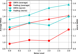
Figure 1: Average and worst-case client RMSE of FedAvg (McMahan et al., 2017) and DRFA (Deng et al., 2021) on a molecular property prediction task.

2 Framework of DRFLM

2.1 Notation

We start by fixing some notations that will be used throughout this paper. we denote $[N]=\{1,2,\cdots,N\}$. We consider federated learning setting where $N$ clients jointly train a central model with the i-th client’s local training datasets of sample size $N_{i}$. The local dataset is denoted as $\mathcal{D}_{i}=\{\bm{z}_{i,j}\}_{j=1}^{N_{i}}$ and each sample $\bm{z}_{i,j}=(\bm{x}_{i,j},y_{i,j})$ is i.i.d. drawn from an unknown local joint distribution $\mathcal{P}_{x,y}^{(i)}$. We denote $Z^{\dagger}$ for any matrix $Z$ as the pseudo inverse of it.

2.2 Optimization Objective

A common used approach in Federated learning (FL) to collaboratively train a central model $\bm{w}$ is to optimize the following objective:

$$\min_{\bm{w}\in\mathcal{W}}F(\bm{w})\coloneqq\sum_{i=1}^{N}\frac{N_{i}}{N}f_{i}(\bm{w})$$ (1)

where $f_{i}(\bm{w})=\frac{1}{N_{i}}\sum_{\bm{z}_{i,j}\in\mathcal{D}_{i}}f(\bm{w},\bm{z}_{i,j})$ is the local empirical risk for client $i$ with the global model. The optimization of Equation 1 suffers from non-iid data distribution, i.e., the heterogeneity across different clients’ data collection (Deng et al., 2021). To provide an intuition, note the target objective in Equation 1 aggregates client-specific loss functions with weights proportional to their local dataset sizes following the standard empirical risk minimization framework. Imbalance sample sizes of different clients or diversity among local data distributions may inevitably plague the generalization ability of the central model obtained by solving Equation 1. To provide the performance guarantee over the worst-case local distribution, Deng et al. (Deng et al., 2021) propose a framework named DRFA to minimize the worst-case combination loss of local empirical distributions:

$$\min_{\bm{w}\in\mathcal{W}}\max_{\bm{\lambda}\in\Lambda}F(\bm{w},\bm{\lambda})=\sum_{i=1}^{N}\lambda_{i}f_{i}(\bm{w})$$ (2)

where $\bm{\lambda}\in\Lambda\coloneqq\{\bm{\lambda}\in\mathbb{R}^{N}_{+},\sum_{i=1}^{N}\lambda_{i}=1\}$ is the learnable sampling weights for each local client and $f_{i}(\cdot)$ is the local empirical distribution.

However, Equation 2 tends to pessimistically optimize the worst-case local distribution which can be easily affected by inter-client data noise. As shown in Figure 1, when we apply these methods to real-world drug discovery datasets, the use of distributionally robust optimization cannot improve the worst-case local RMSE but even significantly reduces the performance.

To mitigate the noise effect on the optimization procedure, instead of directly optimizing the worst-case local empirical distribution, we propose to incorporate the popular data augmentation technique, mixup, into the local training procedure as follows:

$$\min_{\bm{w}\in W}\max_{\bm{\lambda}\in\Lambda}F(\bm{w},\bm{\lambda})\coloneqq\sum_{i=1}^{N}\lambda_{i}\tilde{f}_{i}(\bm{w}).$$ (3)

Here we optimize the worst-case local empirical loss evaluated on the mixup distribution $\tilde{f}_{i}$. To be specific, for the $i$-th client’s local dataset, we denote $\tilde{\bm{x}}^{(i)}_{j,k}(\gamma)=\gamma g(\bm{x}_{i,j})+(1-\gamma)g(\bm{x}_{i,k})$ and $\tilde{y}^{(i)}_{j,k}(\gamma)=\gamma y_{i,j}+(1-\gamma)y_{i,k}$ with $\gamma\in[0,1]$ be the linear interpolation between two samples in the local dataset $\mathcal{D}_{i}$ and $g:\mathbb{R}^{d}\rightarrow\mathbb{R}^{d}$ is a mapping to improve the flexibility of our framework to handle different kinds of data. We choose $g(\cdot)$ as an identity operator for the tableau or image data. For graph prediction tasks including drug discovery, we choose $g(\cdot)$ as a graph neural network to map a graph $(V,E)$ to a global graph embedding in $\mathbb{R}^{d}$. Let $\gamma$ follows the distribution as $\operatorname{Beta}(\alpha,\beta)$, $\tilde{\bm{z}}^{(i)}_{j,k}(\gamma)=(\tilde{\bm{x}}_{j,k}^{(i)}(\gamma),\tilde{y}_{j,k}^{(i)}(\gamma))$ and $\tilde{\mathcal{D}}_{i}(\gamma)=\{\tilde{\bm{z}}^{(i)}_{j,k}(\gamma),j,k\in[N_{i}]\}$ be the local mixup dataset by linear interpolating between every two samples. After the construction of the mix-up empirical distribution, we evaluate each local loss function on the local mixup dataset, i.e., $\tilde{f}_{i}(\bm{w})=\frac{1}{N_{i}^{2}}\sum_{\tilde{\bm{z}}_{j,k}^{(i)}\in\tilde{\mathcal{D}}_{i}(\gamma)}f_{i}(\bm{w},\tilde{\bm{z}}_{j,k}^{(i)})$ and then combine them with learnable sampling weights $\lambda_{i}$ as shown in Equation 3.

2.3 Optimization Procedure

We adopt a similar approach in (Deng et al., 2021) to solve the min-max optimization problem in Equation 3. The core idea is to alternatively update $\bm{w}$ and $\bm{\lambda}$ combining with sample techniques to reduce communication cost. We briefly introduce the main steps in Algorithm 1 (more details can be found in the prior work (Deng et al., 2021)). At the beginning of the $s$-th communication stage, the optimization procedure follows as:

1. Sampling: the server independently selects two subsets of $[N]$, $C_{s}$ and $U_{s}$, both with size of a pre-define parameter $m$ and also samples a time index $t^{{}^{\prime}}_{s}\sim U[0,\tau]$ with a pre-define parameter $\tau$ for updating $\bm{\lambda}$. The selection of $C_{s}$ follows the probability $\bm{\lambda}_{t}\in\mathbb{R}^{N}$ with replacement.

2. Broadcasting: the server broadcasts the central model to the selected clients. Then the client constructs a mixup dataset as discussed above and runs stochastic gradient descent (SGD) algorithm on the mixup dataset to update their local models. After that clients return their local parameter updates after time $t^{{}^{\prime}}_{s}$ (used for updating $\bm{\lambda}$) and the last time $\tau$ (used for updating the global model).

3. Updating $\bar{\bm{w}}_{s+1}$: the server takes an average over the received latest model parameters. To be specific,

   $$\bar{\bm{w}}_{s+1}=\frac{1}{m}\sum_{j\in C_{s}}\mathbf{w}_{s,\tau}^{(j)}$$

4. Updating $\bm{\lambda}_{s+1}$: the server takes an average $\tilde{\mathbf{w}}_{s+1}=\frac{1}{m}\sum_{j\in C_{s}}\mathbf{w}_{s,t^{{}^{\prime}}_{s}}^{(j)}$ and then broadcasts it to all clients in $U_{s}$ and receives the stochastic gradients evaluated at this point to construct an auxiliary vector $\bm{v}_{s}$. Then the server updates $\bm{\lambda}$ as following with some pre-defined learning rate $\eta:$

   $$\bm{\lambda}_{s+1}=\prod_{\bm{\lambda}\in\Lambda}(\bm{\lambda}^{(s)}+\eta\tau\bm{v}_{s}).$$

Algorithm 1 Dristributionally Robust Federated Learning with Local Mixup (DRFLM)

  parameters:

  synchronization gap $\tau$, total communication round $T$, $S=T/\tau$, sampling size $m$, mix-up ratio $\gamma$, initial model $\bar{\bm{w}}_{0}$ and initial weights $\bm{\lambda}_{0}$

  function ClientUpdate($i$, $\bar{\bm{w}}_{s},t_{s}^{{}^{\prime}}$)

  Initialize local weights $\bm{w}_{s,0}^{i}=\bar{\bm{w}}_{s}$

  Construct $\mathcal{\tilde{D}}_{i}(\gamma)=\{\gamma g(\bm{z}_{1})+(1-\gamma)g(\bm{z}_{2})\lvert\bm{z}_{1},\bm{z}_{2}\in\mathcal{D}_{i}\}$

  for $t$ = $1$ to $\tau$ do

     Uniformly sample $\tilde{\bm{z}}_{t}^{(i)}$ from $\mathcal{\tilde{D}}_{i}(\gamma)$

     $\bm{w}_{s,t}^{(i)}=\prod_{\mathcal{W}}\left(\bm{w}_{s,t-1}^{(i)}-\eta\nabla f(\bm{w}_{s,t-1}^{(i)};\tilde{\bm{z}}_{t}^{(i)})\right)$

  end for

  return ($\mathbf{w}_{s,\tau}^{(j)},\mathbf{w}_{s,t^{{}^{\prime}}_{s}}^{(j)}$)

  Server executes:

  initialize $\bar{\bm{w}}_{0}$

  for $s=1$ to $S$ do

     Sample a set $C_{s}\subset[N]$ with size of m and probability $\bm{\lambda}_{s}$ with replacement

     Uniformly sample $t^{{}^{\prime}}_{s}$ from $[\tau]$ uniformly

     Uniformly sample a set $U_{s}\subset[N]$ with size of m

     for client $j\in C_{s}$ in parallel do

        $(\mathbf{w}_{s,\tau}^{(j)},\mathbf{w}_{s,t^{{}^{\prime}}_{s}}^{(j)})=\textsc{ClientUpdate}(j,\bar{\bm{w}}_{s},t_{s}^{{}^{\prime}})$

     end for

     $\bar{\mathbf{w}}_{s+1}=\frac{1}{m}\sum_{j\in C_{s}}\mathbf{w}_{s,\tau}^{(j)}$

     $\tilde{\mathbf{w}}_{s+1}=\frac{1}{m}\sum_{j\in C_{s}}\mathbf{w}_{s,t^{{}^{\prime}}_{s}}^{(j)}$

     Broadcasts $\tilde{\mathbf{w}}_{s+1}$ to all clients $i\in U_{s}$ and receive $f_{i}(\tilde{\mathbf{w}}_{s+1};\tilde{\bm{z}}_{t^{{}^{\prime}}_{s}}^{(i)})$ from local client

     Construct $\bm{v}\in\mathbb{R}^{N}$ with $v_{i}=\frac{N}{m}f_{i}(\tilde{\mathbf{w}}_{s+1};\tilde{\bm{z}}_{t^{{}^{\prime}}_{s}}^{(i)})$ for each indice $i\in U_{s}$ and $v_{i}=0$ for $i\notin U_{s}$

     Updates $\bm{\lambda}_{s+1}=\prod_{\Lambda}(\bm{\lambda}_{s}+\eta\tau\bm{v}_{s})$

  end for

  Output $\bar{\bm{w}}_{S},\bm{\lambda}_{S}$

3 Theoretical Analysis

In this part, we provide different theoretical views to understand our approach in Algorithm 1.

3.1 Theoretical Motivation

We first show a concrete example to demonstrate the effectiveness of our method in mitigating the local noise effect. Specifically, we construct an example as follows:

Example 1.

We consider FL setting with two clients. These two clients jointly train a linear classifier: $\phi(\bm{x};\mathbf{w})=\text{sgn}(\mathbf{w}^{T}\bm{x})$ over the global dataset $(\bm{x},y)$ generated by the joint distribution $P(\bm{x},y)$ as following:

$$\bm{x}\sim P_{X}:=\text{Uniform}\bigg{\{}[-2,-1]^{d}\bigcup\big{(}[1,2]\times[-2,-1]^{d-1}\big{)}\bigg{\}}$$

$$y=\left\{\begin{matrix}1,&x_{1}>0\\ -1,&x_{1}\leq 0\end{matrix}\right..$$

Given the above global joint distribution, the local distribution of each client is defined as following:

• The ”clean” dataset $D_{1}=\{(\bm{x}_{1,i},y_{1,i})\}_{i=1}^{N_{1}}\overset{i.i.d.}{\sim}P(\bm{x},y)$ of the first client is noiseless.

• The ”noisy” dataset $\tilde{D}_{2}=\{(\bm{x}_{2,i},\tilde{y}_{2,i})\}_{i=1}^{N_{2}}\overset{i.i.d.}{\sim}\tilde{P}(\bm{x},\tilde{y})$ ($\tilde{y}$ is a noisy version of $y$ defined as follow):

  $${\tilde{y}}_{2,i}=\left\{\begin{matrix}y_{2,i},&x_{1}\notin I\\ \text{Flipping}(y_{2,i};p_{1}),&x_{1}\in I\end{matrix}\right.$$

  with $I=[-1-p_{2},-1],1/2<p_{1}<1,0<p_{2}<1$ and $\text{Flipping}(y;p_{1})$ the random function that flips $y$ to $-y$ with probability $p_{1}.$ We construct $\tilde{D}_{2}$ as a noisy version of $D_{2}$ to simulate the local noise effect on the training procedure.

Suppose $N_{1}=N_{2}=\tilde{N}$, then given the 0-1 loss $f(\mathbf{w};\bm{x},y):=\bm{1}\{y\neq\phi(\bm{x};\mathbf{w})\}$ and the learned models $\mathbf{w}^{\text{Avg}}_{\tilde{N}},\mathbf{w}^{\text{DRFA}}_{\tilde{N}},\mathbf{w}^{\text{DRFLM}}_{\tilde{N}}$ obtained by minimizing the empirical FedAvg loss (Equation 1), DRFA loss (Equation 2) and DRFLMloss (Equation 3) associated with $\ell$. We then have 

$$\lim_{\tilde{N}\to\infty}\mathbb{E}_{P(\bm{x},y)}[f(\mathbf{w}^{\text{DRFA}}_{\tilde{N}},\bm{x},y)]$$

$$> \lim_{\tilde{N}\to\infty}\mathbb{E}_{P(\bm{x},y)}[f(\mathbf{w}^{\text{Avg}}_{\tilde{N}};\bm{x},y)]$$

$$= \lim_{\tilde{N}\to\infty}\mathbb{E}_{P(\bm{x},y)}[f(\mathbf{w}^{\text{DRFLM}}_{\tilde{N}};\bm{x},y)]=0.$$

As shown by the above inequality, under certain conditions, with the increase of training sample number, losses of FedAvg and our method can gradually decrease to zero while the loss of DRFA cannot converge to zero even with infinity samples. We have two insights from the above example: (1) Directly applying DRO method to FL settings can be easily affected by the local noise. (2) The use of local data mixup has the potential to mitigate the local noise.

3.2 Generalization Guarantee of DRFLM

In previous subsection, we have demonstrated a motivated example to show the effectiveness of local data mixup. In this part, we focus on analyzing the generalization bound of the worst-case client loss in the setting where a generalized linear model is built using our approach. Here, we take generalized linear model as an example and our analysis can be also extended to more complex hypothesis sets such as two-layer neural networks (see more general results in the Appendix B.3):

$$P({y}\lvert\bm{x};\mathbf{w})\propto\exp({y}\mathbf{w}^{T}\bm{x}-\mu(\mathbf{w}^{T}\bm{x}))$$ (4)

with $\bm{x},\mathbf{w}\in\mathbb{R}^{d}$ and $\mu(\cdot)$ is some twice differentiable function. The corresponding negative log likelihood $f$ is:

$$f(\mathbf{w};\bm{x},y)=\mu(\mathbf{w}^{T}\bm{x})-y\mathbf{w}^{T}\bm{x}.$$ (5)

Typical losses such as cross entropy can be obtained by setting different $\mu$. Differentiate $\int P(y\lvert\bm{x};\mathbf{w})dy=1$, we get $\mathbb{E}[y\lvert\bm{x},\mathbf{w}]=\mu^{\prime}(\mathbf{w}^{T}\bm{x})$, thus Equation (4) can be write equivalently as:

$$y=\mu^{\prime}(\mathbf{w}^{T}\bm{x})+\varepsilon,$$ (6)

with $\varepsilon$ as a random variable with zero mean. We further assume that for $\lvert z\rvert\leq 1$ , there exists some $K$ such that

$$K^{-1}\leq\mu^{\prime\prime}(z)\leq K.$$ (7)

In particular, the linear model and the Logistic model satisfies our conditions. Here, we take Linear model for regression as an example: When we set $\mu(z)=\dfrac{1}{2}z^{2},$ Equation (6) turns to be $y=\mathbf{w}^{T}\bm{x}+\varepsilon$, and $f(\mathbf{w};\bm{x},y)=\dfrac{1}{2}(y-\mathbf{w}^{T}\bm{x})^{2}+\dfrac{1}{2}y^{2}$ corresponds to the squared loss. By $\mu^{\prime\prime}(z)=1$, we have $K=1$ satisfies Equation (7).

At a high level, our theory aims to characterize the difference between the population and the empirical (worst-case) losses (i.e., generalization bound of the worst-case loss). The derivation of the generalization bound follows two steps:

• Firstly, we would show that as long as the estimator $\mathbf{w}$ lies in some constrained hypothesis class $\mathcal{W}$, then the generalization ability of $\mathbf{w}$ over the worst-case loss is theoretically guaranteed.

• Then, we argue that the mix-up effect is nearly a penalty that forces the trained estimator fall into the above hypothesis class $\mathcal{W}$.

Step1: Without loss of generality, we denote the $i$-th local dataset as $\mathcal{D}_{i}=\{\bm{z}_{i,j}=(\bm{x}_{i,j},y_{i,j})\}_{j=1}^{N_{i}}$ and assumes $\lVert\bm{x}_{i,j}\rVert_{2},\lVert\mathbf{w}^{*}\rVert_{2}\leq 1.$ We denote

$$\hat{\Sigma}_{i}:=\dfrac{1}{N_{i}}\sum_{j=1}^{N_{i}}\bm{x}_{i,j}\bm{x}_{i,j}^{T},\quad\zeta_{i}(\mathbf{w}):=\dfrac{1}{N_{i}}\sum_{j=1}^{N_{i}}\mu{{}^{\prime\prime}}(\mathbf{w}^{T}\bm{x}_{i,j}),$$

$$\Sigma_{\Lambda}:=\{\sum_{j=1}^{N}\lambda_{i}\hat{\Sigma}_{j}:\lambda\in\Lambda\}.$$

Here $\Sigma_{i}$ and $\hat{\Sigma}_{i}$ denote the population and empirical covariance matrix of the $i$-th client, respectively. We further introduce the following hypothesis class, which can be seen as a federated-setting version of the hypothesis set considered in (Zhang et al., 2021):

$$\mathcal{W}_{r}:=\{\bm{x}\to\mathbf{w}^{T}\bm{x}:\min_{\Sigma\in\Sigma_{\Lambda}}\mathbf{w}^{T}\Sigma\mathbf{w}\leq r\}.$$

In particular, the above hypothesis class involves a quadratic form $\mathbf{w}^{T}\bar{\Sigma}(\mathbf{w})\mathbf{w}$, with

$$\bar{\Sigma}(\mathbf{w}):=\text{argmin}_{\Sigma_{\Lambda}}\{\sum_{i=1}^{N}\lambda_{i}\mathbf{w}^{T}\Sigma_{i}\mathbf{w}\},$$

the weighted average of the data covariance matrices across different clients.

In fact, we will show later that $\mathcal{W}_{r}$ reflect the effect of mix-up comparing with DRFA and FedAvg: Without the mix-up effect, the only information we can infer about the empirical minimizer of DRFA and FedAvg is that $\lVert\mathbf{w}\rVert_{2}\leq 1$, while the DRFLM loss will push its minimizer into $\mathcal{W}_{r}$ due to the mix-up effect, as we will show in Step2. This will provide a more tight generalization bound in most cases.

Now we can show the following generalization bound over the hypothesis class defined above:

Theorem 1 (Generalization Bound of $\mathcal{W}_{r}$).

Suppose $\mu(\cdot)$ is $L$-Lipshitz continuous. Then there exists constants $B>0$ such that for $\mathbf{w}\in\mathcal{W}_{r}$, the following inequality holds with probability $1-\delta$:

$$\max_{\lambda\in\Lambda}\sum_{j=1}^{N}\lambda_{j}\mathbb{E}_{P_{j}(\bm{x},y)}[f(\mathbf{w};\bm{x},y)]$$

$$\leq\max_{\lambda\in\Lambda}\sum_{j=1}^{N}\dfrac{\lambda_{j}}{N_{j}}\sum_{i=1}^{N_{j}}f(\mathbf{w};x_{j}^{i},y_{j}^{i})$$

$$+\max_{\lambda\in\Lambda}\sum_{j=1}^{N}\lambda_{j}\sqrt{\dfrac{1}{N_{j}}}\big{(}\sqrt{\log\dfrac{N}{\delta}}+\sum_{j=1}^{N}rL\cdot{\color[rgb]{1,0,0}\sqrt{H_{j}/N_{j}}}\big{)},$$

with $H_{j}:=\mathbb{E}_{P_{j}}[\max_{\Sigma\in\Sigma_{\Lambda}}\text{tr}\big{(}\Sigma^{\dagger}\hat{\Sigma}_{j}\big{)}]$ .

$H_{j}$ can partially reflects the client heterogeneity from the global distribution. In the IID case, the red part in above inequality turns to be $O(\sqrt{\text{rank}(\Sigma)/N_{j}})$. In contrast, in both FedAvg and DRFA, this term will be $\Omega(\sqrt{d/N_{j}})$. Thus our bound can be more tight when the intrinsic dimension of data is small (i.e., $\text{rank}(\Sigma)\ll d$).

Step2: Now we prove that the learned model obtained by our approach can fall into $\mathcal{W}_{r}(\lambda)$ due to the mixup effect. Employing similar techniques as in (Zhang et al., 2021), we can show that the object function of DRFLM turns approximately to

$$\min_{\mathbf{w}\in W}\max_{\lambda\in\Lambda}\sum_{i=1}^{N}\lambda_{i}({f}_{i}(\mathbf{w})+\underbrace{\dfrac{c}{2}\zeta_{i}(\mathbf{w})\mathbf{w}^{T}\hat{\Sigma}_{i}\mathbf{w}}_{R_{i}(\mathbf{w})}).$$ (8)

Then for any possible $\bm{\lambda}\in\Lambda$ the mixed penalty term $R(\mathbf{w}):=\sum_{i=1}^{N}\lambda_{i}R_{i}(\mathbf{w})$ forces the estimator to enter the set $\mathcal{W}_{r}$ for some $r$. The formal version of the proof is refereed to Appendix 1.

3.3 Convergence analysis

In fact, we can establish similar convergence result for our algorithm 1 under non-convex loss functions by following the proof of Theorem 4 in (Deng et al., 2021) and show that our algorithm can efficiently converge to a stationary point of empirical loss. Following the standard analysis of the nonconvex minimax optimization, we define $\bm{\lambda}^{*}(\mathbf{w})=\operatorname{argmax}_{\bm{\lambda}\in\bm{\Lambda}}F(\mathbf{w},\bm{\lambda})$ and $\Phi(\mathbf{w})=F(\mathbf{w},\bm{\lambda}^{*}(\mathbf{w}))$. To derive meaningful results, the convergence measure concerns the so-called Moreau envelope of $\Phi$ (Moreau, 1965; Davis & Drusvyatskiy, 2019).

Definition 1 (Moreau Envelope).

A function $\Phi_{p}(\bm{x})$ is a $p$-Moreau envelope of a function $\Phi$ if $\Phi_{p}(x)=\min_{\mathbf{w}\in\mathcal{W}}\{\Phi(\mathbf{w})+\frac{1}{2p}\lVert\mathbf{w}-\bm{x}\rVert^{2}\}$.

We use $\frac{1}{2L}$-Moreau envelope of $\Phi$ and the proof is similar to Theorem 2 (Deng et al., 2021) except we apply it on the mixup distribution. For self-containation, the proof is given in Appendix C:

Theorem 2.

Under the assumptions 1-4 in Appendix C and assume the sample space $\mathcal{Z}$ is a convex set, each local function $f_{i}$ is nonconvex, global function $F$ takes the form of our formulation (3), running Algorithm 1 with the choice of $\tau=T^{1/4}$, $\eta=\frac{1}{4LT^{3/4}}$ and $\gamma=\frac{1}{\sqrt{T}}$ we have,

$$\frac{1}{T}\sum_{t=1}^{T}\mathbb{E}\left[\left\|\nabla\Phi_{1/(2L)}\left(\bm{w}^{t}\right)\right\|^{2}\right]$$

$$\leq O\Bigg{(}\frac{D_{\Lambda}^{2}}{T^{1/8}}+\frac{\sigma_{\lambda}^{2}}{mT^{1/4}}+\frac{G_{\lambda}^{2}}{T^{1/4}}$$

$$+\frac{G_{w}\sqrt{G_{w}^{2}+\sigma_{w}^{2}}}{T^{1/8}}+\frac{D_{\mathcal{W}}\left(\sigma_{w}+\sqrt{\Gamma}\right)}{T^{1/2}}\Bigg{)}.$$

4 Experiments

Table 1: The average and worst-case RMSE of client test datasets (lower is better).

Method	Model	ESOL		FreeSolv		Drug Activity
		Average	Worst-case	Average	Worst-case	Average	Worst-case
FedAVG	GCN	$0.976_{(0.072)}$	$1.232_{(0.081)}$	$3.011_{(0.121)}$	$3.863_{(0.104)}$	$0.932_{(0.012)}$	$1.104_{(0.023)}$
	GAT	$1.134_{(0.043)}$	$1.343_{(0.075)}$	$2.641_{(0.431)}$	$3.456_{(0.321)}$	$0.964_{(0.035)}$	$1.197_{(0.032)}$
	MPNN	$0.923_{(0.067)}$	$1.312_{(0.065)}$	$2.974_{(0.669)}$	$3.689_{(0.278)}$	$0.931_{(0.032)}$	$1.231_{(0.035)}$
DRFA	GCN	$1.204_{(0.068)}$	$1.357_{(0.073)}$	$3.465_{(0.264)}$	$3.928_{(0.276)}$	$1.265_{(0.037)}$	$1.542_{(0.029)}$
	GAT	$1.346_{(0.065)}$	$1.466_{(0.046)}$	$2.897_{(0.568)}$	$3.699_{(0.772)}$	$1.323_{(0.027)}$	$1.525_{(0.063)}$
	MPNN	$1.233_{(0.072)}$	$1.386_{(0.064)}$	$3.211_{(0.798)}$	$3.899_{(0.754)}$	$1.148_{(0.043)}$	$1.458_{(0.028)}$
Ours	GCN	$1.086_{(0.056)}$	$1.121_{(0.059)}$	$3.123_{(0.134)}$	$3.532_{(0.096)}$	$1.126_{(0.0480)}$	$1.065_{(0.013)}$
	GAT	$1.243_{(0.049)}$	$1.234_{(0.055)}$	$2.801_{(0.654)}$	$3.207_{(0.441)}$	$1.021_{(0.065)}$	$1.132_{(0.028)}$
	MPNN	$0.989_{(0.054)}$	$1.132_{(0.061)}$	$3.112_{(0.649)}$	$3.579_{(0.489)}$	$0.987_{(0.041)}$	$1.187_{(0.029)}$

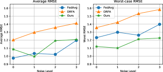
(a) Impact of different noise level.

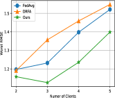
(b) Different client number.

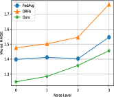
(c) Imbalance mode.

Figure 2: Evaluations under different settings including different noise levels, client number, and imbalance mode.

Most previous work (Deng et al., 2021; Mohri et al., 2019) focus on standard and small-scale academic benchmarks in which most samples are high-quality with negligible data noises. For example, one of the most related work to ours is DRFA (Deng et al., 2021) which conducts experiments on Fashion MNIST. In this paper, we turn to evaluate our method on more challenging tasks in the drug discovery era. Except for drug discovery, we also provide additional results on other applications in the discussion part.

4.1 Setup

Task and Dataset. We consider two typical tasks in drug discovery, molecular property prediction and drug activity prediction. Specifically, molecular property prediction aims to predict ADMET ((absorption, distribution, metabolism, excretion, and toxicity)) properties of a given molecular, which plays a key role in estimating drug candidates’ safety and efficiency. For this task, we select two datasets from the MoleculenNet (Wu et al., 2017) with different properties, namely solubility, and lipophilicity. Drug affinity prediction dataset consists of $34000$ drug molecules and corresponding affinity degrees measured by the IC50 method from the ChEMBL website (Gaulton et al., 2011). The dataset comes from the DrugOOD project (Ji et al., 2022) which provides automated curator and benchmarks for the out-of-distribution problem in drug discovery.

Data Splitting. A key step to evaluate different FL algorithms is data splitting, i.e, splitting the global dataset into different subsets and assigning them to different clients. We consider the non-IID split in this paper. For molecular property prediction, we employ scaffold splitting (Wu et al., 2017) based on scaffolds of molecular graph, which ensures each client has different training distribution (varies in molecular scaffolds). For drug activity prediction, we employ assay splitting based on assay information, which ensures each client have data from different assay setting. Once the client splitting is finished, we split each local dataset into train/validation/test with a ratio $8:1:1$. We gather each local validation set into a global validation set for tuning various hyper-parameters in the training.

Model and Training Setup. In this paper, we select three mainstream GNN models for the above tasks including GCN (Kipf & Welling, 2017), GAT (Veličković et al., 2017) and MPNN (Gilmer et al., 2017). The number of clients is set to $3$ in Table 1. We also provide results of other clients number in Figure 2(b). We set the synchronization gap in Algorithm 1 to $5$ and set the local learning rate to $0.01$. The total training round is set to $100$ for all datasets.

Evaluation Metric. We evaluate DRFLMin terms of average test RMSE and worst-case test RMSE. Average test RMSE denotes the average RMSE of the global model over all local test datasets. This metric can reflect the average model performance on different data distributions. While the worst-case test RMSE is the worst (highest) RMSE among all local test datasets. This metric can partially reflect the model’s generalization ability on different data distributions. For all experiments, as suggested by prior work (Wu et al., 2017), we apply three independent runs on three random seeded scaffold/assay splitting and report the mean and standard deviations.

4.2 Results

The overall results are shown in Table 1. As shown in the table, our method outperforms the previous state-of-the-art method (DRFA (Deng et al., 2021)) on all three datasets in terms of the worst-case RMSE among all clients. For example, in comparison with DRFA, our method has achieved $17\%$ relative reduction of worst-case RMSE on the ESOL dataset owing to the use of mixup (from $1.357$ to $1.121$). We further plot the loss curve of the total training phase in Figure 3 which also shows our method’s superiority in convergence speed. Our method can also outperform the conventional method FedAVG in terms of the worst-case RMSE (1.121 vs 1.232). However, for average RMSE, the performance of our method is slightly worse than FedAVG. Despite the ESOL dataset, our method also shows its superiority in Freesolv and drug activity datasets (see more details in Table 1).

Effects of label noise. From the result, we also observe that conventional FedAVG method consistently outperforms DRFA in terms of both average and worst-case accuracy. This might be caused by the label noise contained in local datasets. To further validate this conjecture, we run three FL methods (FedAvg, DRFA, DRFLM) on noisy datasets whose labels are perturbed by Gaussian noises with different magnitudes. Specifically, we randomly select $50\%$ clients and inject different levels (controlled by standard deviation) of Gaussian noises into their data labels with probability $30\%$. As shown in Figure 2(a), along with the increase of noise level , the worst-case RMSE of DRFA significantly drops which indicates that label noises can easily affect the performance of DRFA. The reason is that DRFA pessimistically optimizes the worst-case combination of local distribution which is typically dominated by the local training distribution with more noises. As a comparison, our method can boost the performance by combining DRFA with the mixup strategy in terms of both average and worst-case RMSE. Note that our method can also achieve better worst-case RMSE than FedAvg. This indicates our method has better generalization ability on different local distributions than conventional FL methods which are appealing to real-world Non-IID settings.

Number of clients. The number of clients is set to $3$ in Table 1. We also provide results on other client number in Figure 2(b). As shown in the figure, our method consistently outperforms the other two methods in all settings in terms of the worst-case RMSE. And in most cases, the increase of the client number leads to significant performance reduction. This may be caused by that we use non-iid splitting in this paper and the increase of client number can increase the model update estimation bias (He et al., 2021). We also note that DRFA achieves similar worst-case RMSE to FedAvg. One possible reason for this might be the decrease in client numbers can reduce the effect of local noises.

Imbalance mode. Previous experiments are all conducted in the balance mode, i.e., the number of samples of each client is the same. In this part, we further evaluate our method under imbalance mode, i.e., the numbers of samples are highly unbalancing among all clients. Specifically, we set the number of clients to 3 and let the sample ratio among these three clients be $7:2:1$. Under the imbalance mode, as shown in Figure 2(c) we observe that the performance of DRFA becomes worse in contrast to the balanced mode. The situation becomes worse with the increase of noise level, which is due to that the client with minimum sample size magnifies the effect of local data noise on the final learned model. Also, our method can still reduce the noise effect under the imbalance mode.

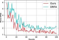
Figure 3: Convergence comparison between ours and DRFA.

Other application. In the above discussions, we evaluate our method on challenging drug discovery tasks. To give a more comprehensive evaluation of our method, we further conduct experiments on some academic benchmarks including Fashion MNIST and UCI Adults, which are commonly used in previous work (Deng et al., 2021; Mohri et al., 2019). Following the setting of prior work (Mohri et al., 2019), we extract the subset of the data labeled with different labels and split this subset into three local datasets, and assign them to different clients. For Fashion MNIST, the subsets are set to t-shirt/top, pullover, and shirt following the prior work (Mohri et al., 2019). For the Adult dataset, we set subsets to doctorate and non-doctorate. The training round is set to $1000$, the overall results are shown in Table 2. From this table, we observe that DRFA outperforms all other two methods on the FMNIST dataset in terms of worst-case accuracy. One possible explanation is that the Fashion MNIST dataset contains high-quality labeled samples thus there is no noise that can affect the training procedure. This can be verified by conducting experiment on the ”flipped” dataset, i.e., flipping the training samples’ label with probability $30\%$. For the Fashion MNIST with label flipping, the performance of DRFA becomes worse than the others methods including ours. The performance drop can be caused by the injected flipping noise. Moreover, our method can significantly boost the worst-case classification accuracy by using mixup to reduce the noise effect.

Table 2: The worst-case classification accuracy of FMNIST and Adult datasets. Flip means flipping the training samples’ label with a given probability.

Dataset	FedAvg	DRFA	Ours
FMNIST	$70.64_{(0.212)}$	$71.04_{(0.321)}$	$70.89_{(0.234)}$
Adult	$68.21_{(0.187)}$	$67.31_{(0.256)}$	$69.87_{(0.268)}$
FMNIST+Flip	$67.21_{(0.342)}$	$66.28_{(0.439)}$	$69.78_{(0.376)}$
Adult+Flip	$66.23_{(0.232)}$	$64.86_{(0.314)}$	$68.66_{(0.321)}$

5 Related Works

5.1 Distributionally Robust Optimization

Distributionally robust optimization is a general learning paradigm that enforcing the learned model to perform well over the local worst-case risk functions. Generally, the local worst-case risk function refers to the supremum of the risk function over ambiguity set which is a vicinity of the empirical data distribution (Duchi et al., 2011). Data distributions contained in the ambiguity set have small distances to the true empirical data distribution wherein the distance is computed based on well-known probability metrics such as $\phi$-divergence and wasserstein distance (Wang et al., 2021). Although DRO can be always formulated as a minimax optimization problem, in most real-world cases, exactly solving this minimax problem is intractable since it involves the supremum over infinite many probability distributions, thus two streams of literature to handle it by using either a primal-dual pair of infinite-dimensional linear programs (Esfahani & Kuhn, 2018) or first-order optimality conditions of the dual. Amongst them, the most related to us is (Namkoong & Duchi, 2016), which proposes an efficient bandit mirror descent algorithm for the minimax problem when the uncertainty set is constructed using $f$-divergence.

5.2 Federated Learning on Non-IID Data

There is a rich body of literatures aims to modify the conventional FL method for solving inter-client data heterogeneity (Non-IID issue). One typical way to improve FedAvg on the Non-iid setting is to employ different local training strategies for different clients (Li et al., 2020b, a; Reddi et al., 2021). We call this line of work adaptive federated learning since they need to either adaptively adjust the local learning rate or modify the local empirical loss function by adding a client-aware regularizer. For example, Scaffold (Karimireddy et al., 2020) identifies that the performance degradation of FedAvg on Non-iid data is caused by ”client drift” issue. and introduces extra device variables to adaptively adjust the local loss. A more general and essential way to overcome the client heterogeneity is to incorporate distributionally robust optimization (DRO) (Kwon et al., 2020; Zhai et al., 2021; Duchi et al., 2011) into conventional FL paradigm (Mohri et al., 2019; Deng et al., 2021). DRFA (Deng et al., 2021) is a recent work that proposes to optimize the agnostic (distributionally robust) empirical loss, which combines different local loss functions with learnable weights. This method theoretically ensures that the learned model can perform well over the worst-case local loss combination. Previous work in this line has shown its effectiveness in deep neural networks on some small-scale benchmarks (e.g., Fashion MNIST).

6 Conclusion

In this paper, we propose a general framework which simultaneously mitigate the inter-client data heterogeneity (i.e., Non-IID issue) and the intra-client data noise. We provide comprehensive theoretical analysis of the proposed approach. We also apply our method to real-world drug discovery tasks and show the superiority of our method in reducing the local noise effects. Our results show: (1)Directly applying DRO methods to FL settings suffers poor performance caused by intra-client data noise. (2) Combining mixup strategy with DRO can mitigate the noise side effects. Despite FL, our framework can be employed in other scenarios, e.g., fair machine learning. The future work includes improving the theoretical properties of mixup in the FL setting. Another interesting direction would be exploring the cross-client mixup strategy (i.e., mixup data from different clients).

In this appendix, Section A gives an detailed exploration on Example 1 to illustrate why DRFA may fail in the federated learning setting while our proposed DRFLMcan rescue. Section B provide the formal proof for the Theorem 1. Section C presents the proof for our DRFLM’s optimization guarantee (Theorem 2) and the associated assumptions. Section B.3 is an extension for Theorem 1.

Appendix A Proofs for Counter-Examples

A.1 One-Dimensional Example of ERM

To prove our statements in Example 1, we first study the following one-dimensional example: Consider $P_{x,y}$ defined as following:
i) The margin distribution $P_{x}$ is uniform on intervals $[-2,-1]\cup[1,2]$
ii) Condition on $x$, $P(y\lvert x)=1-2\cdot\bm{1}\{x\leq 0\}$
Consider the ERM procedure over the function classes $\mathcal{F}:=\{f_{x}(z):=1-2\cdot\bm{1}\{z<x\}\}$, we have in noiseless case the excess risk of the ERM estimator will converge to $0$ as sample-size increasing. Similar as in Example 1, for $1/2<p_{1}<1$ we define $I=[-2,-1]$, and suppose the random perturbation is given in form of flipping labels for $x\in I$ with probability $p_{1}$, then as sample-size increasing there will be $p_{1}$-ratio of samples has label $1$ in the interval $I$. As a result, we have then the decision boundary of ERM estimator will turns to the left-boundary point of $I$, i.e. $-2$, thus will have excess risk $1/2>0.$ While if we consider the all-sample mix-up with constant mixture factor $1/2$, then as sample-size increasing the mixed up sample turns to distributed as following:
i) $1/4$ ratio samples lies between $[1,2]$ with label $1$,
ii) $1/2$ ratio samples lies between $[-1,1]$ with label $\dfrac{1}{2}$ with probability $1-p_{1}$ and $1$ with probability $p$,
iii) $1/4$ ratio samples lies between $[-2,-1]$ with label $1$ with probability $p^{2}$ ,$\dfrac{1}{2}$ with probability $2p(1-p)$ and $0$ with probability $(1-p)^{2}$.
Now a classifier with decision boundary at $x_{0}=-2$ will incur the least squared error$\frac{1}{4}(1-p)+\frac{1}{2}p(1-p)+\frac{1}{4}p^{2}=\frac{1}{2}$ while a classifier with decision boundary at $x_{0}=-1$ will incur the least squared error $\dfrac{1}{4}p^{2}+\dfrac{1}{2}p(1-p)<1/2$ whenever $p>1/2$. Thus the ERM estimator over the mixed up distribution will select its decision boundary at the right-hand-side of $-1$, thus gives $0$ population risk.

A.2 Proof of Statements in Example 1

Now we consider the Example 1: Firstly, notice that in this example, $\Lambda=\{\bm{\lambda}\in\mathbb{R}^{2}_{+},\sum_{i=1}^{2}\lambda_{i}=1\}$, thus the empirical FedAvg, empirical DRFA loss, and the empirical DRFLMloss and are given by $\frac{1}{2}(f_{1}(\mathbf{w})+f_{2}(\mathbf{w})),\max_{i\in\{1,2\}}f_{i}(\mathbf{w}),\max_{i\in\{1,2\}}\tilde{f}_{i}(\mathbf{w})$. Noticing that as sample-size increasing, we have for $\mathbf{w}$ with decision boundary of $f(\bm{x};\mathbf{w})$ lies in $-2<b<2$ will incur the following empirical loss:

$$f_{1}(\mathbf{w}) =-\dfrac{1+b}{2}\cdot\bm{1}\{b<-1\}+\dfrac{b-1}{2}\cdot\bm{1}\{b>1\}.$$

$$f_{2}(\mathbf{w}) =(\dfrac{(1-p_{1})p_{2}}{2}-\dfrac{1+p_{2}+b}{2})\cdot\bm{1}\{b<-1-p_{2}\}+(\dfrac{b-1}{2}+\dfrac{p_{1}p_{2}}{2})\cdot\bm{1}\{b>1\}...$$

$$+(-\dfrac{b+1}{2}(1-p_{1})+\dfrac{b+1+p_{2}}{2}p_{1})\bm{1}\{b\in I\}.$$

Thus by elementary calculation, we have as ${\tilde{N}}\to\infty$, the decision boundary corresponding to $f(\bm{x};\mathbf{w}_{\tilde{N}}^{\text{DRFA}})$ will turn to $-1-p_{2}.$ On the other hand, we can show that the the decision boundary corresponding to $f(\bm{x};\mathbf{w}_{\tilde{N}}^{\text{Avg}})$ can be any point in $[-1,1]$.

Finally, analyze the decision boundary of $f(\bm{x};\mathbf{w}_{\tilde{N}}^{\text{DRFLM}})$, we first assume as in example in section A.1 that the mix-up of two data $\bm{x},\bm{x}^{\prime}$ is given by $\dfrac{1}{2}(\bm{x}+\bm{x}^{\prime})$, such simplification will not loss the generality because it equals to the in-expectation value of mixed-up data when $\alpha=\beta.$ Firstly, notice that for client $1$, we have obviously that for $\mathbf{w}_{1}$ the empirical-risk-minimizer of $\tilde{f}_{1}(\mathbf{w}),$ its decision boundary lies between $[-1,1]$. For client $2$, we have when looking at the first coordinate, there are fewer samples with label $-1$ when $x_{1}\leq 1$ than the one-dimensional example in section A.1, thus the decision boundary of corresponding empirical risk minimizer of $\tilde{f}(\mathbf{w})$ will in the right hand side of the decision boundary of mixed-up ERM considered in section A.1, i.e. it will in the right hand side of $-1$. That shows $\tilde{f}_{2}(\mathbf{w})$ also encourage its minimizer to lie in $[-1,2]$. As a consequence, we have the decision boundary of the ERM of $\max_{i\in\{1,2\}}\tilde{f}_{i}(\mathbf{w})$ will lie in $[-1,2]$ as ${\tilde{N}}\to\infty$, which will has zero population risk.

Appendix B Proofs for Generalization Guarantee

B.1 Mix-Up Effect for Generalizaed Linear Model

Using the Lemma 3.3 in (Zhang et al., 2021), we have for $f(\mathbf{w};\bm{x},y)=\mu(\mathbf{w}^{T}\bm{x})-y\mathbf{w}^{T}\bm{x}$ and $f_{j}(\mathbf{w})=\dfrac{1}{N_{j}}\sum_{i=1}^{N_{j}}f(\mathbf{w};x_{j}^{i},y_{j}^{i})$, when $\sum_{j}x_{j}^{i}=0$, the second order approximation of DRFLMloss is given by

$$\min_{\mathbf{w}\in W}\max_{\lambda\in\Lambda}\sum_{i=1}^{N}\lambda_{i}({f}_{i}(\mathbf{w})+\underbrace{\dfrac{c}{2}\zeta_{i}(\mathbf{w})\mathbf{w}^{T}\hat{\Sigma}_{i}\mathbf{w}}_{R_{i}(\mathbf{w})})$$

with $c=\mathbb{E}_{\gamma\sim D_{\gamma}}[\dfrac{(1-\gamma)^{2}}{\gamma^{2}}]$ and $D_{\gamma}=\dfrac{\alpha}{\alpha+\beta}\text{Beta}(\alpha+1,\beta)+\dfrac{\alpha}{\alpha+\beta}\text{Beta}(\beta+1,\alpha).$ Now recall the assumption that $K^{-1}\leq\lvert\mu^{\prime\prime}(z)\rvert\leq K$, we get then $\zeta_{i}(\mathbf{w})\geq K^{-1}$ , thus for any $\lambda\in\Lambda$ we have

$$\sum_{i=1}^{N}\lambda_{i}\dfrac{c}{2}\zeta_{i}(\mathbf{w})\mathbf{w}^{T}\hat{\Sigma}_{i}\mathbf{w}\geq\min_{\lambda\in\Lambda}\sum_{i=1}^{N}\lambda_{i}\dfrac{c}{2K}\mathbf{w}^{T}\hat{\Sigma}_{i}\mathbf{w}.$$

By $\lVert x_{j}^{i}\rVert_{2},\mathbf{w}\leq 1$, we have for $\hat{\mathbf{w}}$ the minimizer of DRFLM,

$$\sum_{i=1}^{N}\lambda_{i}\dfrac{c}{2K}\hat{\mathbf{w}}^{T}\hat{\Sigma}_{i}\hat{\mathbf{w}}\leq\dfrac{cK}{2}.$$

i.e. $\hat{w}\in\mathcal{W}_{r}$ with $r=K^{2}$.

B.2 Proof of Theorem 1

We first establish the following standard uniform deviation bound result based on the Rademacher complexity, which is an analogue of Theorem 10 of (Mohri et al., 2019):

Lemma 1.

Assuming the loss function $\ell$ is bounded by $M$. Fix $\epsilon>0$ and $\mathbf{n}:=(n_{1},\dots,n_{m})$. Then for any $\delta>0$, with probability at least $1-\delta$ over the draw of samples $D_{j}\sim P_{j}^{N_{j}}$, the following inequality holds for all $\phi\in\mathcal{F}$ and $\lambda\in\Lambda$:

$$\sum_{j=1}^{m}\lambda_{j}\mathbb{E}_{P_{j}}[\ell(f(x),y)] \leq\sum_{j=1}^{N}\dfrac{\lambda_{j}}{N_{j}}\sum_{i=1}^{N_{j}}\ell(\phi(x_{i}^{j}),y_{i}^{j})$$

$$+\sum_{j=1}^{N}\lambda_{j}\big{(}\mathcal{R}^{j}_{N_{j}}(\mathcal{F})+M\sqrt{\dfrac{\log(N/\delta)}{2N_{j}}}\big{)}$$

where

$$\mathcal{R}^{j}_{N_{j}}(\mathcal{F})=\mathbb{E}_{D_{j}}\big{[}\mathbb{E}_{\varepsilon}[\sup_{\phi\in\mathcal{F}}\dfrac{1}{N_{j}}\sum_{i=1}^{N_{j}}\varepsilon_{ij}\ell(\phi(x_{i}^{j},y^{j}_{i}))]\big{]}.$$

Proof of the Lemma.

Recall that by Theorem 8 of (Bartlett & Mendelson, 2003), for any $M$-uniformly bounded and $L$-Lipschitz function $\ell$, for all $\phi\in\mathcal{F}$, with probability at least $1-\delta,$

$$\mathbb{E}[\ell(\phi(x),y)]\leq\dfrac{1}{n}\sum_{i=1}^{n}\ell(\phi(x_{i}),y_{i})+2L\mathcal{R}_{n}(\mathcal{F})+M\sqrt{\dfrac{\log(1/\delta)}{2n}}$$

Now applying this result to each client $j$ and use the union bound leads to the desired result. ∎

Proof of Theorem 1 .

To apply the lemma, we need to compute the empirical Rademacher complexity $\mathcal{R}_{N_{j}}^{j}(\mathcal{F};D_{j})$ firstly:

$$\mathcal{R}_{N_{j}}^{j}(\mathcal{W}_{r};D_{j}) :=\mathbb{E}_{\varepsilon}[\sup_{w\in\mathcal{W}_{r}}\dfrac{1}{N_{j}}\sum_{i=1}^{N_{j}}\varepsilon_{ij}\mathbf{w}^{T}x_{i}^{j}]$$

$$=\mathbb{E}_{\varepsilon}[\sup_{\mathbf{w}^{T}\bar{\Sigma}(\mathbf{w})\mathbf{w}\leq r}\dfrac{1}{N_{j}}\sum_{i=1}^{N_{j}}\varepsilon_{ij}\mathbf{w}^{T}x_{i}^{j}]$$

$$=\mathbb{E}_{\varepsilon}[\sup_{\mathbf{w}^{T}\bar{\Sigma}(\mathbf{w})\mathbf{w}\leq r}\dfrac{1}{N_{j}}\sum_{i=1}^{N_{j}}\varepsilon_{ij}\mathbf{w}^{T}\bar{\Sigma}(\mathbf{w})^{1/2}\big{(}\bar{\Sigma}(\mathbf{w})^{1/2}\big{)}^{\dagger}x_{i}^{j}]$$

$$\leq r\mathbb{E}_{\varepsilon}[\sup_{\mathbf{w}^{T}\bar{\Sigma}(\mathbf{w})\mathbf{w}\leq r}\dfrac{1}{N_{j}}\big{\lVert}\sum_{i=1}^{N_{j}}\varepsilon_{ij}\big{(}\bar{\Sigma}(\mathbf{w})^{1/2}\big{)}^{\dagger}x_{i}^{j}\big{\rVert}]$$

$$\leq\dfrac{r}{{N_{j}}}\sqrt{\mathbb{E}_{\varepsilon}[\sup_{\Sigma\in\Sigma_{\Lambda}}\big{\lVert}\sum_{i=1}^{N_{j}}\varepsilon_{ij}\Sigma^{\dagger}x_{i}^{j}\big{\rVert}^{2}]}$$

$$\leq\dfrac{r}{{N_{j}}}\sqrt{\sup_{\Sigma\in\Sigma_{\Lambda}}\sum_{i=1}^{N_{j}}(x_{i}^{j})^{T}\Sigma^{\dagger}x_{i}^{j}}$$

Now noticing

$$\mathcal{R}_{N_{j}}^{j}(\mathcal{W}_{r}) =\mathbb{E}_{D_{j}}[\mathcal{R}_{N_{j}}^{j}(\mathcal{F};D_{j})]$$

$$\leq\dfrac{r}{\sqrt{N_{j}}}\cdot\sqrt{\mathbb{E}[\dfrac{1}{N_{j}}\sup_{\Sigma\in\Sigma_{\Lambda}}\sum_{i=1}^{N_{j}}(x_{i}^{j})^{T}\Sigma^{\dagger}x_{i}^{j}]}$$

and applying Lemma 1 leads to the desired result. ∎

B.3 Extending to Non-linear case

As in (Zhang et al., 2021), our analysis for generalized linear model can also be extended to the second-layer neural network with squared loss: In that case $f(\mathbf{w};\bm{x},y)=\big{(}y-\theta_{1}^{T}\sigma(W\bm{x})-\theta_{0}\big{)}^{2}$ with $\theta_{1}\in\mathbb{R}^{p},\theta_{0}\in\mathbb{R},W\in\mathbb{R}^{p\times d}$ and $\mathbf{w}$ consists of $\theta_{1},\theta_{0},W)$ . If we perform mixup on the second layer and assume without loss of generality that $\{\sigma(Wx^{j}_{i})\}_{i=1}^{N_{j}}$ are centered, then by Lemma 3.4 of (Zhang et al., 2021), we have the second order approximation of DRFLM  loss is given by

$$\min_{\mathbf{w}\in W}\max_{\lambda\in\Lambda}\sum_{i=1}^{N}\lambda_{i}({f}_{i}(\mathbf{w})+{\dfrac{c}{2}\zeta_{i}(\mathbf{w})\mathbf{w}^{T}\hat{\Sigma}_{i}^{\sigma}\mathbf{w}}),$$

where $\hat{\Sigma}_{i}^{\sigma}$ is the sample covariance of $\sigma(Wx^{j}_{i})$ of $i$-th client. Using the same argument as in GLM case, we have such loss forces its minimizer lies in

$$\mathcal{W}_{r}^{\sigma}:=\{\bm{x}\to\theta_{1}^{T}\sigma(W\bm{x})+\theta_{0}:\min_{\lambda\in\Lambda}\sum_{i=1}^{N}\lambda_{i}\theta_{1}^{T}\hat{\Sigma}_{i}^{\sigma}\theta_{1}\leq r\}$$

for some $r$. To study the generalization ability, notice that by the similar argument as in generalized linear setting, we have

$$\mathcal{R}^{j}_{N_{j}}(\mathcal{W}_{r}^{\sigma})\leq\dfrac{r}{\sqrt{N_{j}}}\cdot\sqrt{\mathbb{E}[\sup_{\Sigma\in\Sigma^{\sigma}_{\Lambda}}\sum_{i=1}^{N_{j}}\text{tr}(\Sigma^{\dagger}\hat{\Sigma}^{\sigma}_{j})]}.$$

Where $\Sigma^{\sigma}_{\Lambda}=\{\sum_{j=1}^{N}\lambda_{i}\hat{\Sigma}_{j}^{\sigma}:\lambda\in\Lambda\}$. Now apply the Lemma 1 leads to the following formal result:

Theorem 3 (Generalization Bound of $\mathcal{W}_{r}^{\sigma}$).

Suppose both $\theta_{1},W,\theta_{0}$ are bounded, then there exists constants $L,B>0$ such that for $\mathbf{w}\in\mathcal{W}_{r}^{\sigma}$, the following inequality holds with probability $1-\delta$:

$$\max_{\lambda\in\Lambda}\sum_{j=1}^{N}\lambda_{j}\mathbb{E}_{P_{j}(\bm{x},y)}[f(\mathbf{w};\bm{x},y)]$$

$$\leq\max_{\lambda\in\Lambda}\sum_{j=1}^{N}\dfrac{\lambda_{j}}{N_{j}}\sum_{i=1}^{N_{j}}f(\mathbf{w};x_{j}^{i},y_{j}^{i})+\max_{\lambda\in\Lambda}\sum_{j=1}^{N}\lambda_{j}\sqrt{\dfrac{1}{N_{j}}}\big{(}\sqrt{\log\dfrac{N}{\delta}}$$

$$+\sum_{j=1}^{N}rL\cdot{\color[rgb]{1,0,0}\sqrt{\big{(}H_{j}^{\sigma}\big{)}/N_{j}}}\big{)}.$$

with $H_{j}^{\sigma}:=\mathbb{E}_{P_{j}}[\max_{\Sigma\in\Sigma^{\sigma}_{\Lambda}}\text{tr}\big{(}\Sigma^{\dagger}\hat{\Sigma}_{j}^{\sigma}\big{)}]$

Appendix C Optimization Guarantee

Assumption 1 (Weighted Gradient Dissimilarity).

A set of local objectives $f_{i}(\cdot),i=1,2,\ldots,N$ exhibit $\Gamma$ gradient dissimilarity defined as $\Gamma:=\sup_{\bm{w}\in\mathcal{W},\bm{\lambda}\in\Lambda,i\in[n]},\sum_{j\in[n]}\lambda_{j}\left\|\nabla f_{i}(\bm{w})-\nabla f_{j}(\bm{w})\right\|^{2}.$

Assumption 2.

The gradient w.r.t $\bm{w}$ and $\bm{\lambda}$ are bounded, i.e., $\left\|\nabla f_{i}(\bm{w})\right\|\leq$ $G_{w}$ and $\left\|\nabla_{\bm{\lambda}}F(\bm{w},\bm{\lambda})\right\|\leq G_{\lambda}$.

Assumption 3.

The diameters of $\mathcal{W}$ and $\Lambda$ are bounded by $D_{\mathcal{W}}$ and $D_{\Lambda}$.

Assumption 4.

Let $\hat{\nabla}F(\bm{w};\bm{\lambda})$ be a stochastic gradient for $\bm{\lambda}$, which is the $N$-dimensional vector such that the $i$-th entry is $f_{i}(\mathbf{w};\bm{z})$, and the rest are zero. Then we assume $\left\|\nabla f_{i}(\bm{w};\bm{z})-\nabla f_{i}(\bm{w})\right\|\leq\sigma_{w}^{2},\forall i\in[N],\bm{z}\in\mathcal{Z}$ and $\|\hat{\nabla}F(\bm{w};\bm{\lambda})-\nabla F(\bm{w};\bm{\lambda})\|\leq\sigma_{\lambda}^{2}$.

Lemma 2 (One iteration analysis (Deng et al., 2021)).

Under the assumptions 1-4, the following statement holds for algorithm 1:

$$\mathbb{E}\left[\Phi_{1/2L}\left(\bar{\bm{w}}_{t}\right)\right]\leq\mathbb{E}\left[\Phi_{1/2L}\left(\bar{\bm{w}}_{t-1}\right)\right]+2\eta D_{\mathcal{W}}L^{2}\mathbb{E}\left[\frac{1}{m}\sum_{i\in\mathcal{D}^{\lfloor\frac{t-1}{\tau}\rfloor}}\left\|\bm{w}^{(i)}_{t-1}-\bar{\bm{w}}_{t-1}\right\|\right]$$

$$+2\eta L\left(\mathbb{E}\left[\Phi\left(\bar{\bm{w}}_{t-1}\right)\right]-\mathbb{E}\left[F\left(\bm{w}_{t-1},\bm{\lambda}_{\lfloor\frac{t-1}{\tau}\rfloor}\right)\right]\right)-\frac{\eta}{4}\mathbb{E}\left[\left\|\nabla\Phi_{1/(2L)}\left(\bar{\bm{w}}_{t-1}\right)\right\|^{2}\right].$$

Lemma 3 (Bounded Norm Deviation) (Deng et al., 2021)).

$\forall i\in C_{\lfloor\frac{t}{\tau}\rfloor}$, the norm distance between $\bar{\bm{w}}_{t}$ and $\bm{w}^{(i)}_{t}$ is bounded as follows:

$$\frac{1}{T}\sum_{t=0}^{T}\mathbb{E}\left[\frac{1}{m}\sum_{i\in C_{\lfloor\frac{t}{\tau}\rfloor}}\left\|\bm{w}^{(i)}_{t}-\bar{\bm{w}}_{t}\right\|\right]\leq 2\eta\tau\left(\sigma_{w}+\frac{\sigma_{w}}{m}+\sqrt{\Gamma}\right).$$

Lemma 4 (Lemma 9, (Deng et al., 2021)).

For algorithm 1, under the assumptions 1-4, the following statement holds true:

$$\frac{1}{T}\sum_{t=1}^{T}\left(\mathbb{E}\left[\Phi\left(\bar{\bm{w}}_{t}\right)\right]-\mathbb{E}\left[F\left(\bar{\bm{w}}_{t},\bm{\lambda}_{\lfloor\frac{t}{\tau}\rfloor}\right)\right]\right)\leq 2\sqrt{S}\tau\eta G_{w}\sqrt{G_{w}^{2}+\sigma_{w}^{2}}+\gamma\tau\frac{\sigma_{\lambda}^{2}}{m}+\gamma\tau G_{\lambda}^{2}+\frac{D_{\Lambda}^{2}}{2\sqrt{S}\tau\gamma}.$$

Proof of Theorem 2

Proof.

From lemma 2 we know,

$$\frac{1}{T}\sum_{t=1}^{T}\mathbb{E}\left[\|\nabla\Phi_{1/2L}\right. \left.\left(\bar{\bm{w}}_{t}\right)\|^{2}\right]$$

$$\leq \frac{4}{\eta T}\mathbb{E}\left[\Phi_{1/(2L)}\left(\bar{\bm{w}}_{0}\right)\right]+\frac{D_{\mathcal{W}}L^{2}}{2T}\sum_{t=1}^{T}\mathbb{E}\left[\frac{1}{m}\sum_{i\in C_{\lfloor\frac{t}{\tau}\rfloor}}\left\|\bm{w}^{(i)}_{t}-\bar{\bm{w}}_{t}\right\|\right]$$

$$+\frac{L}{2T}\sum_{t=1}^{T}\left(\mathbb{E}\left[\Phi\left(\bar{\bm{w}}_{t}\right)\right]-\mathbb{E}\left[F\left(\bar{\bm{w}}_{t},\bm{\lambda}_{\lfloor\frac{t}{\tau}\rfloor}\right)\right]\right).$$

Plugging in Lemma 3 and 4 yields:

$$\frac{1}{T}\sum_{t=1}^{T}\mathbb{E}\left[\left\|\nabla\Phi_{1/(2L)}\left(\bar{\bm{w}}_{t}\right)\right\|^{2}\right]\leq \frac{4}{\eta T}\mathbb{E}\left[\Phi_{1/(2L)}\left(\bar{\bm{w}}_{0}\right)\right]+\eta\tau D_{\mathcal{W}}L^{2}\left(\sigma_{w}+\frac{\sigma_{w}}{m}+\sqrt{\Gamma}\right)$$

$$+\sqrt{S}\tau\eta G_{w}L\sqrt{G_{w}^{2}+\sigma_{w}^{2}}+\gamma\tau\frac{\sigma_{\lambda}^{2}L}{2m}+\gamma\tau\frac{G_{\lambda}^{2}L}{2}+\frac{D_{\Lambda}^{2}L}{4\sqrt{S}\tau\gamma}.$$

Plugging in $\eta=\frac{1}{4LT^{3/4}},\gamma=\frac{1}{T^{1/2}}$ and $\tau=T^{1/4}$ we obtain the convergence rate as cliamed:

$$\frac{1}{T}\sum_{t=1}^{T}\mathbb{E}\left[\left\|\nabla\Phi_{1/(2L)}\left(\bar{\bm{w}}_{t}\right)\right\|^{2}\right]\leq \frac{4}{T^{1/4}}\mathbb{E}\left[\Phi_{1/2L}\left(\bm{w}_{0}\right)\right]+\frac{L^{2}}{T^{1/2}}\left(\sigma_{w}+\frac{\sigma_{w}}{m}+\sqrt{\Gamma}\right)$$

$$+\frac{1}{T^{1/8}}G_{w}L\sqrt{G_{w}^{2}+\sigma_{w}^{2}}+\frac{\sigma_{\lambda}^{2}L}{2mT^{1/4}}+\frac{G_{\lambda}^{2}L}{2T^{1/4}}+\frac{D_{\Lambda}^{2}L}{4T^{1/8}}.$$

Note that here the expectation takes over the randomness incurred by the mixup sampling. ∎

References

- Bartlett & Mendelson (2003) Bartlett, P. L. and Mendelson, S. Rademacher and gaussian complexities: Risk bounds and structural results. J. Mach. Learn. Res., 3(null):463–482, mar 2003. ISSN 1532-4435.
- Bento et al. (2014) Bento, A. P., Gaulton, A., Hersey, A., Bellis, L. J., Chambers, J., Davies, M., Krüger, F. A., Light, Y., Mak, L., McGlinchey, S., et al. The chembl bioactivity database: an update. Nucleic acids research, 42(D1):D1083–D1090, 2014.
- Chen et al. (2020a) Chen, C., Li, L., Wu, B., Hong, C., Wang, L., and Zhou, J. Secure social recommendation based on secret sharing. In Giacomo, G. D., Catalá, A., Dilkina, B., Milano, M., Barro, S., Bugarín, A., and Lang, J. (eds.), ECAI 2020 - 24th European Conference on Artificial Intelligence, 29 August-8 September 2020, Santiago de Compostela, Spain, August 29 - September 8, 2020 - Including 10th Conference on Prestigious Applications of Artificial Intelligence (PAIS 2020), volume 325 of Frontiers in Artificial Intelligence and Applications, pp. 506–512. IOS Press, 2020a. doi: 10.3233/FAIA200132. URL https://doi.org/10.3233/FAIA200132.
- Chen et al. (2020b) Chen, C., Zhou, J., Wu, B., Fang, W., Wang, L., Qi, Y., and Zheng, X. Practical privacy preserving POI recommendation. ACM Trans. Intell. Syst. Technol., 11(5):52:1–52:20, 2020b. doi: 10.1145/3394138. URL https://doi.org/10.1145/3394138.
- Chen et al. (2021) Chen, S., Xue, D., Chuai, G., Yang, Q., and Liu, Q. FL-QSAR: a federated learning-based QSAR prototype for collaborative drug discovery. Bioinform., 36(22-23):5492–5498, 2021. doi: 10.1093/bioinformatics/btaa1006. URL https://doi.org/10.1093/bioinformatics/btaa1006.
- Davis & Drusvyatskiy (2019) Davis, D. and Drusvyatskiy, D. Stochastic model-based minimization of weakly convex functions. SIAM Journal on Optimization, 29(1):207–239, 2019.
- Deng et al. (2021) Deng, Y., Kamani, M. M., and Mahdavi, M. Distributionally Robust Federated Averaging. arXiv:2102.12660 [cs, stat], February 2021. URL http://arxiv.org/abs/2102.12660. arXiv: 2102.12660.
- Duchi et al. (2011) Duchi, J., Hazan, E., and Singer, Y. Adaptive subgradient methods for online learning and stochastic optimization. Journal of machine learning research, 12(7), 2011.
- Esfahani & Kuhn (2018) Esfahani, P. M. and Kuhn, D. Data-driven distributionally robust optimization using the wasserstein metric: Performance guarantees and tractable reformulations. Mathematical Programming, 171(1):115–166, 2018.
- Gaulton et al. (2011) Gaulton, A., Bellis, L. J., Bento, A. P., Chambers, J., Davies, M., Hersey, A., Light, Y., McGlinchey, S., Michalovich, D., Al-Lazikani, B., and Overington, J. P. ChEMBL: a large-scale bioactivity database for drug discovery. Nucleic Acids Research, 40(D1):D1100–D1107, 09 2011. ISSN 0305-1048. doi: 10.1093/nar/gkr777. URL https://doi.org/10.1093/nar/gkr777.
- Gilmer et al. (2017) Gilmer, J., Schoenholz, S. S., Riley, P. F., Vinyals, O., and Dahl, G. E. Neural message passing for quantum chemistry. In Precup, D. and Teh, Y. W. (eds.), Proceedings of the 34th International Conference on Machine Learning, ICML 2017, Sydney, NSW, Australia, 6-11 August 2017, volume 70 of Proceedings of Machine Learning Research, pp. 1263–1272. PMLR, 2017. URL http://proceedings.mlr.press/v70/gilmer17a.html.
- He et al. (2021) He, C., Balasubramanian, K., Ceyani, E., Rong, Y., Zhao, P., Huang, J., Annavaram, M., and Avestimehr, S. Fedgraphnn: A federated learning system and benchmark for graph neural networks. CoRR, abs/2104.07145, 2021. URL https://arxiv.org/abs/2104.07145.
- Ji et al. (2022) Ji, Y., Zhang, L., Wu, J., Wu, B., Huang, L.-K., Xu, T., Rong, Y., Li, L., Ren, J., Xue, D., Lai, H., Xu, S., Feng, J., Liu, W., Luo, P., Zhou, S., Huang, J., Zhao, P., and Bian, Y. DrugOOD: Out-of-Distribution (OOD) Dataset Curator and Benchmark for AI-aided Drug Discovery – A Focus on Affinity Prediction Problems with Noise Annotations. arXiv e-prints, art. arXiv:2201.09637, January 2022.
- Karimireddy et al. (2020) Karimireddy, S. P., Kale, S., Mohri, M., Reddi, S. J., Stich, S. U., and Suresh, A. T. SCAFFOLD: stochastic controlled averaging for federated learning. In Proceedings of the 37th International Conference on Machine Learning, ICML 2020, 13-18 July 2020, Virtual Event, volume 119 of Proceedings of Machine Learning Research, pp. 5132–5143. PMLR, 2020. URL http://proceedings.mlr.press/v119/karimireddy20a.html.
- Kipf & Welling (2017) Kipf, T. N. and Welling, M. Semi-supervised classification with graph convolutional networks. In 5th International Conference on Learning Representations, ICLR 2017, Toulon, France, April 24-26, 2017, Conference Track Proceedings. OpenReview.net, 2017. URL https://openreview.net/forum?id=SJU4ayYgl.
- Kwon et al. (2020) Kwon, Y., Kim, W., Won, J.-H., and Paik, M. C. Principled learning method for Wasserstein distributionally robust optimization with local perturbations. In International Conference on Machine Learning, pp. 5567–5576. PMLR, November 2020. URL https://proceedings.mlr.press/v119/kwon20a.html. ISSN: 2640-3498.
- Li et al. (2020a) Li, T., Sahu, A. K., Zaheer, M., Sanjabi, M., Talwalkar, A., and Smith, V. Federated optimization in heterogeneous networks. In Dhillon, I. S., Papailiopoulos, D. S., and Sze, V. (eds.), Proceedings of Machine Learning and Systems 2020, MLSys 2020, Austin, TX, USA, March 2-4, 2020. mlsys.org, 2020a. URL https://proceedings.mlsys.org/book/316.pdf.
- Li et al. (2021) Li, T., Hu, S., Beirami, A., and Smith, V. Ditto: Fair and robust federated learning through personalization. In Meila, M. and Zhang, T. (eds.), Proceedings of the 38th International Conference on Machine Learning, ICML 2021, 18-24 July 2021, Virtual Event, volume 139 of Proceedings of Machine Learning Research, pp. 6357–6368. PMLR, 2021. URL http://proceedings.mlr.press/v139/li21h.html.
- Li et al. (2020b) Li, X., Huang, K., Yang, W., Wang, S., and Zhang, Z. On the convergence of fedavg on non-iid data. In International Conference on Learning Representations, 2020b. URL https://openreview.net/forum?id=HJxNAnVtDS.
- McMahan et al. (2017) McMahan, B., Moore, E., Ramage, D., Hampson, S., and y Arcas, B. A. Communication-efficient learning of deep networks from decentralized data. In Singh, A. and Zhu, X. J. (eds.), Proceedings of the 20th International Conference on Artificial Intelligence and Statistics, AISTATS 2017, 20-22 April 2017, Fort Lauderdale, FL, USA, volume 54 of Proceedings of Machine Learning Research, pp. 1273–1282. PMLR, 2017. URL http://proceedings.mlr.press/v54/mcmahan17a.html.
- Mendez et al. (2019) Mendez, D., Gaulton, A., Bento, A. P., Chambers, J., De Veij, M., Félix, E., Magariños, M. P., Mosquera, J. F., Mutowo, P., Nowotka, M., et al. Chembl: towards direct deposition of bioassay data. Nucleic acids research, 47(D1):D930–D940, 2019.
- Mohri et al. (2019) Mohri, M., Sivek, G., and Suresh, A. T. Agnostic Federated Learning. In Proceedings of the 36th International Conference on Machine Learning, pp. 4615–4625. PMLR, May 2019. URL https://proceedings.mlr.press/v97/mohri19a.html. ISSN: 2640-3498.
- Moreau (1965) Moreau, J.-J. Proximité et dualité dans un espace hilbertien. Bulletin de la Société mathématique de France, 93:273–299, 1965.
- Namkoong & Duchi (2016) Namkoong, H. and Duchi, J. C. Stochastic gradient methods for distributionally robust optimization with f-divergences. In NIPS, volume 29, pp. 2208–2216, 2016.
- Reddi et al. (2021) Reddi, S. J., Charles, Z., Zaheer, M., Garrett, Z., Rush, K., Konečný, J., Kumar, S., and McMahan, H. B. Adaptive federated optimization. In International Conference on Learning Representations, 2021. URL https://openreview.net/forum?id=LkFG3lB13U5.
- Reisizadeh et al. (2020) Reisizadeh, A., Farnia, F., Pedarsani, R., and Jadbabaie, A. Robust Federated Learning: The Case of Affine Distribution Shifts. arXiv:2006.08907 [cs, math, stat], June 2020. URL http://arxiv.org/abs/2006.08907. arXiv: 2006.08907.
- Sheller et al. (2020) Sheller, M. J., Edwards, B., Reina, G. A., Martin, J., Pati, S., Kotrotsou, A., Milchenko, M., Xu, W., Marcus, D., Colen, R. R., et al. Federated learning in medicine: facilitating multi-institutional collaborations without sharing patient data. Scientific reports, 10(1):1–12, 2020.
- Veličković et al. (2017) Veličković, P., Cucurull, G., Casanova, A., Romero, A., Lio, P., and Bengio, Y. Graph attention networks. arXiv preprint arXiv:1710.10903, 2017.
- Wang et al. (2021) Wang, Y., Wang, W., Liang, Y., Cai, Y., and Hooi, B. Mixup for Node and Graph Classification. In Proceedings of the Web Conference 2021, pp. 3663–3674, Ljubljana Slovenia, April 2021. ACM. ISBN 978-1-4503-8312-7. doi: 10.1145/3442381.3449796. URL https://dl.acm.org/doi/10.1145/3442381.3449796.
- Wu et al. (2017) Wu, Z., Ramsundar, B., Feinberg, E. N., Gomes, J., Geniesse, C., Pappu, A. S., Leswing, K., and Pande, V. S. Moleculenet: A benchmark for molecular machine learning. CoRR, abs/1703.00564, 2017. URL http://arxiv.org/abs/1703.00564.
- Xie et al. (2021) Xie, H., Ma, J., Xiong, L., and Yang, C. Federated graph classification over non-iid graphs. CoRR, abs/2106.13423, 2021. URL https://arxiv.org/abs/2106.13423.
- Xiong et al. (2020) Xiong, Z., Cheng, Z., Liu, X., Wang, D., Luo, X., Chen, K., Jiang, H., and Zheng, M. Facing small and biased data dilemma in drug discovery with federated learning. BioRxiv, 2020.
- Yang et al. (2019) Yang, Q., Liu, Y., Chen, T., and Tong, Y. Federated machine learning: Concept and applications. ACM Trans. Intell. Syst. Technol., 10(2):12:1–12:19, 2019. doi: 10.1145/3298981. URL https://doi.org/10.1145/3298981.
- Zhai et al. (2021) Zhai, R., Dan, C., Kolter, Z., and Ravikumar, P. DORO: Distributional and Outlier Robust Optimization. In Proceedings of the 38th International Conference on Machine Learning, pp. 12345–12355. PMLR, July 2021. URL https://proceedings.mlr.press/v139/zhai21a.html. ISSN: 2640-3498.
- Zhang et al. (2021) Zhang, L., Deng, Z., Kawaguchi, K., Ghorbani, A., and Zou, J. How Does Mixup Help With Robustness and Generalization? arXiv:2010.04819 [cs, stat], March 2021. URL http://arxiv.org/abs/2010.04819. arXiv: 2010.04819.