MMV-Based Sequential AoA and AoD Estimation for Millimeter Wave MIMO Channels

Abstract

The fact that the millimeter-wave (mmWave) multiple-input multiple-output (MIMO) channel has sparse support in the spatial domain has motivated recent compressed sensing (CS)-based mmWave channel estimation methods, where the angles of arrivals (AoAs) and angles of departures (AoDs) are quantized using angle dictionary matrices. However, the existing CS-based methods usually obtain the estimation result through one-stage channel sounding that have two limitations: (i) the requirement of large-dimensional dictionary and (ii) unresolvable quantization error. These two drawbacks are irreconcilable; improvement of the one implies deterioration of the other. To address these challenges, we propose, in this paper, a two-stage method to estimate the AoAs and AoDs of mmWave channels. In the proposed method, the channel estimation task is divided into two stages, Stage I and Stage II. Specifically, in Stage I, the AoAs are estimated by solving a multiple measurement vectors (MMV) problem. In Stage II, based on the estimated AoAs, the receive sounders are designed to estimate AoDs. The dimension of the angle dictionary in each stage can be reduced, which in turn reduces the computational complexity substantially. We then analyze the successful recovery probability (SRP) of the proposed method, revealing the superiority of the proposed framework over the existing one-stage CS-based methods. We further enhance the reconstruction performance by performing resource allocation between the two stages. We also overcome the unresolvable quantization error issue present in the prior techniques by applying the atomic norm minimization method to each stage of the proposed two-stage approach. The simulation results illustrate the substantially improved performance with low complexity of the proposed two-stage method.

I Introduction

The spectrum-rich millimeter-wave (mmWave) frequencies between $30-300$ GHz have the potential to alleviate the current spectrum crunch in sub-6GHz bands that service providers are already experiencing. This major potential of the mmWave band has made it one of the most important components of future mobile cellular and emerging WiFi networks. However, due to significant differences between systems operating in mmWave and legacy sub-6 GHz bands, providing reliable and low-delay communication in the mmWave bands is extremely challenging. Specifically, to achieve the high spectral efficiency of mmWave communications, accurate channel state information (CSI) is the key [1, 2, 3, 4, 5], which is, however, challenging due to the high dimensionality of the channel as well as the mmWave hardware constraints.

Nevertheless, the mmWave multiple-input multiple-output (MIMO) channel exhibits sparse property [6, 7], facilitating the sparse channel representation by using small numbers of the angles of arrivals (AoAs), angles of departures (AoDs), and path gains. Typically, by approximating the AoAs and AoDs to be on quantized angle grids, the compressed sensing (CS)-based approaches transform the AoA and AoD estimation problem to a sparse signal recovery problem [8, 9], where the transmitter sends the channel sounding beams to the receiver and the receiver jointly estimates AoAs and AoDs. We refer to this method as the one-stage channel sounding scheme. In particular, due to easy implementation and amenability for analysis, the orthogonal matching pursuit (OMP) has been widely studied [9, 10, 11, 12, 13]. The OMP iteratively searches a pair of AoA and AoD over an over-complete dictionary. However, the computational complexity of OMP increases quadratically with the sizes of the dictionaries, i.e., $O(LKG_{r}G_{t})$, where $K$ is the number of channel uses for the channel sounding, $L$ is the number of channel paths, and $G_{r}$ and $G_{t}$ are the dimensions of angle dictionaries for AoA and AoD, respectively. It is worth pointing out that when the dimensions of the over-complete dictionaries, i.e., $G_{r}$ and $G_{t}$, increase, the complexity of the one-stage CS-based methods such as OMP becomes exceedingly impractical.

The over-complete dictionary and high computational complexity issues have been addressed in an adaptive-CS point-of-view with the primary focus on the sensing vector adaptation to the previous observations [3, 8, 14]. Theoretically, it has been shown that the adaptive CS can be benificial in low SNR [15]. The multi-level (hierarchical) AoA and AoD search techniques [3, 8] leveraged the feedback, where the receiver conveys a feedback to the transmitter to guide the next level angle dictionary design. It is worth noting that these adaptation methods [3, 8] need multiple feedbacks and its performance critically relies on the reliability of the feedback. To reduce the feedback overhead, a two-stage CS was proposed in [14], where the first stage is to obtain a coarse estimation of the support set and the second stage refines the result of the first stage. This method [14] only requires one-time feedback, but achieves compatible estimation performance in low SNR.

I-A Our Contributions

We newly study a sequential, two-stage AoA and AoD estimation framework for reduced computational complexity and improved estimation performance. Specifically, in Stage I, the support set of AoAs is recovered at the receiver by solving a multiple measurement vectors (MMV) problem. Leveraging the shared sparse set, it has been found that the MMV approach can provide improved estimation performance compared to the single measurement vector (SMV) approach [16, 17, 18]. In Stage II, the receiver estimates the AoDs of the channel by exploiting the estimated AoAs from Stage I. Importantly, the estimated AoAs guide the design of receive sounding signals, which saves the channel use overhead and improves the accuracy of AoD estimation. In each stage, since we only estimate AoAs or AoDs, the dimensions of the signal and angle dictionary are much smaller than those of the one-stage joint AoA and AoD estimation [9, 11, 12], readily reducing the computational complexity substantially. This can be viewed as of converting the multiplicative channel sounding overhead (e.g., ${\mathcal{O}}(G_{r}G_{t})$ of OMP) to an additive overhead.

By analyzing the MMV statistics, we present a lower bound for the successful probability of recovering the support sets. Furthermore, based on the successful recovery probability (SRP) analysis of the proposed two-stage method, a resource allocation (between Stage I and Stage II) strategy is newly proposed to improve SRPs for both AoA and AoD estimation. The numerical results validate the efficacy of the proposed resource allocation method.

Finally, in order to address the issue of unresolvable quantization error, we extend the proposed two-stage method to the one with super resolution. Specifically, in each stage of AoA or AoD estimation, we reformulate the MMV problem as an atomic norm minimization problem [19, 20, 21], which is solved by using alternating direction method of multipliers (ADMM). Compared to the dictionary-based methods, the atomic norm minimization can be thought of as the case when the infinite dictionary matrix is employed. We demonstrate through simulations that the quantization error of the two-stage method with super resolution can be effectively reduced.

I-B Paper Organization and Notations

The paper is organized as follows. In Section II, we introduce the signal model and the CS-based channel estimation problem. In Section III, based on the angular-domain channel representation, the proposed sequential AoA and AoD estimation method is presented. In Section IV, we analyze the proposed method in terms of SRP and introduce the resource allocation strategy. In Section V, the atomic norm-based design is described, which resolves the quantization error in the estimated AoAs and AoDs. The simulation results and conclusion are presented in Section VI and Section VII, respectively.

Notations: A bold lower case letter $\mathbf{a}$ is a vector and a bold capital letter $\mathbf{A}$ is a matrix. ${{\mathbf{A}}^{T}}$, ${{\mathbf{A}}^{*}}$, ${{\mathbf{A}}^{H}}$, ${{\mathbf{A}}^{-1}}$, $\operatorname{tr}(\mathbf{A})$, $\left|\mathbf{A}\right|$, ${{\left\|\mathbf{A}\right\|}_{F}}$ and ${{\left\|\mathbf{a}\right\|}_{2}}$ are, respectively, the transpose, conjugate, Hermitian, inverse, trace, determinant, Frobenius norm of $\mathbf{A}$, and $\ell_{2}$-norm of $\mathbf{a}$. $\mathbf{A}^{\dagger}=(\mathbf{A}^{H}\mathbf{A})^{-1}\mathbf{A}^{H}$ denotes the pseudo inverse of a tall matrix $\mathbf{A}$. ${{[\mathbf{A}]}_{:.i}}$, ${{[\mathbf{A}]}_{i,:}}$, ${{[\mathbf{A}]}_{i,j}}$, and $[\mathbf{a}]_{i}$ are, respectively, the $i$th column, $i$th row, $i$th row and $j$th column entry of $\mathbf{A}$, and $i$th entry of vector $\mathbf{a}$. $\mathrm{\mathop{vec}}(\mathbf{A})$ stacks the columns of $\mathbf{A}$ and forms a long column vector. $\mathrm{\mathop{diag}}(\mathbf{a})$ returns a square diagonal matrix with the vector $\mathbf{a}$ on the main diagonal. ${{\mathbf{I}}_{M}}\in{{\mathbb{R}}^{M\times M}}$ is the $M$-dimensional identity matrix. The $\mathbf{1}_{M,N}\in{\mathbb{R}}^{M\times N}$ and $\mathbf{0}_{M,N}\in{\mathbb{R}}^{M\times N}$ are the all one matrix, and zero matrix, respectively. ${\mathcal{R}}(\mathbf{F})$ denotes the subspace spanned by the columns of matrix $\mathbf{F}$. $\mathbf{A}\otimes\mathbf{B}$ and $\mathbf{A}\circ\mathbf{B}$ denote the Kronecker product and Khatri-Rao product of $\mathbf{A}$ and $\mathbf{B}$, respectively. The $\lceil x\rceil$ returns the smallest integer greater than or equal to $x$.

II System Model and General Statement of Techniques

II-A Channel Model

The mmWave transmitter and receiver are equipped with $N_{t}$ and $N_{r}$ antennas, respectively. Suppose that the number of separable paths between the transmitter and receiver is $L$, where $L\ll\min\{N_{r},N_{t}\}$. The physical mmWave channel representation based on the uniform linear array [22, 9, 23, 24] is given by,

$$\mathbf{H}=\sqrt{\frac{N_{r}N_{t}}{L}}\sum\limits_{l=1}^{L}{{{\alpha}_{l}}}\mathbf{a}_{r}({f_{r,l}}){\mathbf{a}_{t}^{H}}({f_{t,l}}),$$ (1)

where $\mathbf{a}_{t}(\cdot)\in{\mathbb{C}}^{N_{t}\times 1}$ and $\mathbf{a}_{r}(\cdot)\in{\mathbb{C}}^{N_{r}\times 1}$ are the array response vectors of the transmit and receive antenna arrays. Specifically, $\mathbf{a}_{t}(f)$ and $\mathbf{a}_{r}(f)$ are given by $\mathbf{a}_{t}(f)=\frac{1}{\sqrt{N_{t}}}{{\left[1,{{e}^{j2\pi f}},\ldots,{{e}^{j2\pi(N_{t}-1)f}}\right]}^{T}}$ and $\mathbf{a}_{r}(f)=\frac{1}{\sqrt{N_{r}}}{{\left[1,{{e}^{j2\pi f}},\ldots,{{e}^{j2\pi(N_{r}-1)f}}\right]}^{T}}$, where $f\in[0,1)$ is the normalized spatial angle. Here we assume ${{f}_{r,l}}$ and ${{f}_{t,l}}$ in (1) are independent and uniformly distributed in $[0,1)$, and the gain of the $l$th path $\alpha_{l}$ follows the complex Gaussian distribution, i.e., ${{\alpha}_{l}}\sim\mathcal{C}\mathcal{N}(0,\sigma_{l}^{2})$. Angular domain representation of the channel in (1) can be rewritten as

$$\mathbf{H}={{\mathbf{A}}_{r}}\operatorname{diag}(\mathbf{h})\mathbf{A}_{t}^{H},$$ (2)

where ${{\mathbf{A}}_{r}}=[\mathbf{a}_{r}({{f}_{r,1}}),\ldots,\mathbf{a}_{r}({{f}_{r,L}})]\in{\mathbf{C}^{N_{r}\times L}}$ , ${{\mathbf{A}}_{t}}=[\mathbf{a}_{t}({{f}_{t,1}}),\ldots,\mathbf{a}_{t}({{f}_{t,L}})]\in{\mathbf{C}^{N_{t}\times L}}$, and $\mathbf{h}=[h_{1},\ldots,h_{L}]\in{\mathbb{C}}^{L\times 1}$ with $h_{l}=\sqrt{\frac{N_{r}N_{t}}{L}}{{\alpha}_{l}}$, $l=1,\ldots,L$.

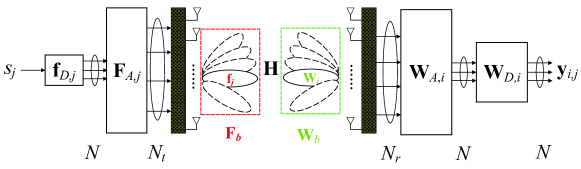
Fig. 1: Conventional one-stage mmWave channel sounding

II-B Channel Sounding

Fig. 1 illustrates the conventional one-stage mmWave channel sounding operation, where the transmitter and receiver are equipped with the large-dimensional hybrid analog-digital MIMO arrays that are driven by a limited number of RF chains, i.e., $N\ll\min\{N_{t},N_{r}\}$. In each channel use of downlink channel sounding, the transmitter generates a beam conveying the pilot signal and the receiver simultaneously generates $N$ separate beams, using the $N$ RF chains, to obtain a $N$-dimensional observation. We let the numbers of the transmit sounding beams (TSBs) and receive sounding beams (RSBs) for channel estimation be $B_{t}$ and $B_{r}$, respectively. For convenience, we assume that $B_{r}$ is an integer multiple of $N$. The total number of channel uses for the conventional one-stage sounding process is then $K=B_{r}B_{t}/N$. Specifically, the RSB matrix in Fig. 1 is given by

$$\mathbf{W}_{b}=[{\mathbf{W}_{1}},{\mathbf{W}_{2}},\ldots,{\mathbf{W}_{B_{r}/N}}]\in{\mathbf{C}^{N_{r}\times{B_{r}}}},$$ (3)

where $\mathbf{W}_{i}\in{\mathbf{C}^{N_{r}\times N}}$ for $i=1,2,\ldots,B_{r}/N$, and $\mathbf{W}_{i}=\mathbf{W}_{A,i}\mathbf{W}_{D,i}$ with $\mathbf{W}_{A,i}\in{\mathbf{C}^{N_{r}\times N}}$ and $\mathbf{W}_{D,i}\in{\mathbf{C}^{N\times N}}$ being the receive analog and digital sounders, respectively. Similarly, the TSB matrix is given by

$$\mathbf{F}_{b}=[{{\mathbf{f}}_{1}},{{\mathbf{f}}_{2}},\cdots,{\mathbf{f}}_{B_{t}}]\in{\mathbf{C}^{N_{t}\times{B_{t}}}},$$ (4)

where $\mathbf{f}_{j}\in{\mathbf{C}^{N_{t}\times 1}}$ for $j=1,2,\cdots,B_{t}$ is the $j$th transmit sounder, and $\mathbf{f}_{j}={\mathbf{F}_{A,j}}{\mathbf{f}_{D,j}}s_{j}$ with ${\mathbf{F}_{A,j}}\in{\mathbf{C}^{N_{t}\times N}}$ and $\mathbf{f}_{D,j}\in{\mathbf{C}^{N\times 1}}$ being the transmit analog and digital sounders, respectively. Each observation $\mathbf{y}_{i,j}\in{\mathbb{C}}^{N\times 1}$ in Fig. 1, associated with the $i$th RSB and $j$th TSB, $i\in\{1,\ldots,B_{r}/N\}$ and $j\in\{1,2,\ldots,B_{t}\}$, can be expressed as

$${\mathbf{y}}_{i,j}=\mathbf{W}_{i}^{H}\mathbf{H}{{\mathbf{f}}_{j}}s_{j}+\mathbf{W}_{i}^{H}{{\mathbf{n}}_{j}}.$$ (5)

The $s_{j}$ denotes the training signal and without loss of generality, we let $s_{j}=1$. It is worth noting that only phase shifters are employed to constitute the analog arrays for power saving, where $|{{[{\mathbf{W}_{A,i}}]}_{m,n}}|=1/\sqrt{N_{r}}$, and $|{{[{\mathbf{F}_{A,j}}]}_{m,n}}|=1/\sqrt{N_{t}},\forall\,m,n$. Moreover, the power constraint $\left\|{{\mathbf{f}}_{j}}\right\|_{2}^{2}=p$ is imposed to the transmit sounding beam at each channel use with $p$ being the power budget, and the noise vector follows ${{\mathbf{n}}_{j}}\sim\mathcal{C}\mathcal{N}(\mathbf{0}_{N_{r}},{{\sigma}^{2}}{{\mathbf{I}}_{N_{r}}})$. Thus, the signal to noise ratio is $p/{{\sigma}^{2}}$.

We collect all observations in (5) by using $\mathbf{W}_{b}$ in (3) and $\mathbf{F}_{b}$ in (4) as

$$\mathbf{Y}={\mathbf{W}_{b}^{H}}\mathbf{H}\mathbf{F}_{b}+{\mathbf{W}_{b}^{H}}\mathbf{N},$$ (6)

where $\mathbf{Y}\in{\mathbb{C}}^{B_{r}\times B_{t}}$ and $\mathbf{N}=[\mathbf{n}_{1},\ldots,\mathbf{n}_{B_{t}}]\in{\mathbb{C}}^{N_{r}\times B_{t}}$. For example, $\mathbf{W}_{b}$ and $\mathbf{F}_{b}$ in (6) can be generated randomly [4] or designed as a partial discrete Fourier transform (DFT) matrix [9]. We assume that the number of observations is strictly lower than the dimension of the channel matrix, i.e., ${B_{r}}{B_{t}}\ll N_{r}N_{t}$. The channel estimation task is to utilize the observations in (5) (equivalently, (6)) to obtain the estimate of the channel matrix $\mathbb{H}$ in (2). Encountering (2), the channel estimation task boils down to reconstructing $\{{{f}_{r,1}},\ldots,{{f}_{r,L}}\}$, $\{{{f}_{t,1}},\ldots,{{f}_{t,L}}\}$ and $\{{{h}_{1}},\ldots,{{h}_{L}}\}$ from the observations.

II-B1 Oracle Estimator

The oracle estimator that we will utilize for benchmark is obtained by assuming perfect knowledge of AoAs and AoDs in (2). The oracle channel estimate only needs to estimate the path gain $\mathbf{h}$, thus the channel estimate is expressed as $\widehat{\mathbf{H}}=\mathbf{A}_{r}\operatorname{diag}(\widehat{\mathbf{h}})\mathbf{A}_{t}^{H}$, where $\operatorname{diag}(\widehat{\mathbf{h}})\in{\mathbb{C}}^{L\times 1}$ is the solution to the following problem:

$$\widehat{\mathbf{h}}=\operatorname*{arg\,min}_{\mathbf{h}}\|\mathbf{Y}-{\mathbf{W}_{b}^{H}}\mathbf{A}_{r}\operatorname{diag}({\mathbf{h}})\mathbf{A}_{t}^{H}\mathbf{F}_{b}\|_{F}^{2}.$$ (7)

Because (7) is convex, the optimal solution is $\widehat{\mathbf{h}}=(\mathbf{X}^{H}\mathbf{X})^{-1}\mathbf{X}^{H}\operatorname{vec}(\mathbf{Y})$, where $\mathbf{X}\in{\mathbb{C}}^{B_{r}B_{t}\times L}$ is given by $\mathbf{X}=\left[\operatorname{vec}{([\mathbf{W}_{b}^{H}\mathbf{A}_{r}]_{:,1}[\mathbf{A}_{t}^{H}\mathbf{F}_{b}]_{1,:})},\ldots,\operatorname{vec}{([\mathbf{W}_{b}^{H}\mathbf{A}_{r}]_{:,L}[\mathbf{A}_{t}^{H}\mathbf{F}_{b}]_{L,:})}\right]$. Because we have $B_{r}B_{t}\gg L$, $\mathbf{X}^{H}\mathbf{X}$ is invertible.

II-C Compressed Sensing-Based Channel Estimation

Recalling the channel model in (2), a typical CS framework restricts the normalized spatial angles ${{f}_{r,l}},{{f}_{t,l}},~{}l=1,2,\ldots,L$, to be chosen from the discrete angle dictionaries, ${{f}_{r,l}}\in\left[0,{1}/{G_{r}},\ldots,{(G_{r}-1)}/{G_{r}}\right]$, and ${{f}_{t,l}}\in\left[0,{1}/{G_{t}},\ldots,{(G_{t}-1)}/{G_{t}}\right]$, where $G_{r}=\lceil sN_{r}\rceil$ and $G_{t}=\lceil sN_{t}\rceil$ with $s\geq 1$ are, respectively, the cardinalities of the receive and transmit spatial angle dictionaries. The transmit and receive array response dictionaries are then given by

$$~{}~{}~{}\bar{\mathbf{A}}_{r}=\left[\mathbf{a}_{r}(0),\mathbf{a}_{r}\left(\frac{1}{G_{r}}\right),\ldots,\mathbf{a}_{r}\left(\frac{G_{r}-1}{G_{r}}\right)\right]\in{\mathbf{C}^{N_{r}\times G_{r}}}$$

and

$$~{}~{}~{}\bar{\mathbf{A}}_{t}=\left[\mathbf{a}_{t}(0),\mathbf{a}_{t}\left(\frac{1}{G_{t}}\right),\ldots,\mathbf{a}_{t}\left(\frac{G_{t}-1}{G_{t}}\right)\right]\in{\mathbf{C}^{N_{t}\times G_{t}}}.$$

For the latter array response dictionaries, the channel model in (2) can be rewritten as

$$\mathbf{H}=\bar{\mathbf{A}}_{r}{\bar{\mathbf{H}}_{a}}\bar{\mathbf{A}}_{t}^{H}+\mathbf{E},$$ (8)

where ${\bar{\mathbf{H}}_{a}}\in{\mathbf{C}^{G_{r}\times G_{t}}}$ is an $L$-sparse matrix with $L$ non-zero entries corresponding to the positions of AoAs and AoDs on their respective angle grids, and $\mathbf{E}\in{\mathbb{C}}^{N_{r}\times N_{t}}$ denotes the quantization error.

Because the dictionary matrices $\bar{\mathbf{A}}_{r}$ and $\bar{\mathbf{A}}_{t}$ are known, the channel estimation task is equivalent to estimating the non-zero entries in $\bar{\mathbf{H}}_{a}$. Plugging the model in (8) into (6) gives

$$\mathbf{Y}={\mathbf{W}_{b}^{H}}\bar{\mathbf{A}}_{r}({\bar{\mathbf{H}}_{a}}+\mathbf{E})\bar{\mathbf{A}}_{t}^{H}\mathbf{F}_{b}+{\mathbf{W}_{b}^{H}}\mathbf{N}.$$ (9)

Vectorizing $\mathbf{Y}$ in (9) yields

$$\operatorname{vec}(\mathbf{Y}) =({\mathbf{F}_{b}^{T}}\bar{\mathbf{A}}_{t}^{*}\otimes{\mathbf{W}_{b}^{H}}\bar{\mathbf{A}}_{r})(\operatorname{vec}({\bar{\mathbf{H}}_{a}}+\mathbf{E}))+\operatorname{vec}({\mathbf{W}_{b}^{H}}\mathbf{N}).$$ (10)

Denoting $\mathbf{D}={\mathbf{F}_{b}^{T}}\bar{\mathbf{A}}_{t}^{*}\otimes{\mathbf{W}_{b}^{H}}\bar{\mathbf{A}}_{r}\in{\mathbf{C}^{{B_{r}}{B_{t}}\times G_{r}{{G}_{b}}}}$ and $\bar{\mathbf{n}}=\mathbf{D}\operatorname{vec}(\mathbf{E})+\operatorname{vec}({\mathbf{W}_{b}^{H}}\mathbf{N})\in{\mathbf{C}^{{B_{r}}{B_{t}}\times 1}}$ gives $\operatorname{vec}(\mathbf{Y})=\mathbf{D}\operatorname{vec}({\bar{\mathbf{H}}_{a}})+\bar{\mathbf{n}}$. Hence, the estimation of $\operatorname{vec}({\bar{\mathbf{H}}_{a}})$ from (10) can be stated as a sparse signal reconstruction problem:

$$\min_{\bar{\mathbf{H}}_{a}}\|\operatorname{vec}(\mathbf{Y})-\mathbf{D}\operatorname{vec}({\bar{\mathbf{H}}_{a}})\|_{2}~{}\text{subject to }\|\operatorname{vec}({\bar{\mathbf{H}}_{a}})\|_{0}=L,$$ (11)

where $\|\cdot\|_{0}$ is the $\ell_{0}$-norm that returns the number of non-zero coordinates of a vector. The problem in (11) can be solved by using standard CS methods [28, 29].

The number of required observations to reconstruct $L$-sparse vector $\operatorname{vec}(\bar{\mathbf{H}}_{a})\in{\mathbb{C}}^{G_{r}G_{t}\times 1}$ in (11) has previously characterized as $O\left(L\cdot\log(G_{r}G_{t})\right)$ [28], which is much smaller than $O(N_{r}N_{t})$. However, the computational complexity for estimating $\operatorname{vec}(\bar{\mathbf{H}}_{a})$ in (11) by using OMP, for example, is $O(LB_{r}B_{t}G_{r}G_{t})$. Though the quantization error associated with using dictionaries can be made small by increasing the sizes of the dictionaries, the growing computational complexity remains a critical challenge. Instead of developing another one-stage channel sounding method (as in Fig. 1), we propose a new two-stage channel sounding and estimation framework to overcome the large overhead and complexity drawbacks.

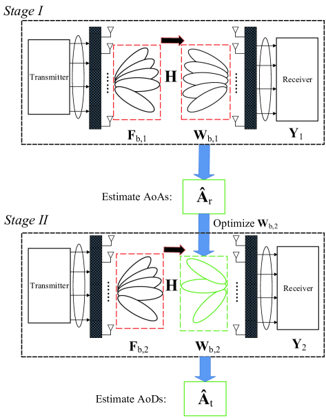
Fig. 2: Illustration of the proposed two-stage AoA and AoD estimation.

III Two-stage AoA and AoD Estimation

A conceptual diagram of the proposed two-stage AoA and AoD estimation framework is presented in Fig. 2. The proposed sequential technique has constituent two stages of channel sounding, where each stage exclusively exploits much low-dimensional dictionary compared to the one-stage channel sounding in Fig. 1.

Under the similar definitions of one-stage method in (6), in Stage I of the two-stage framework of Fig. 2, the transmit and receive sounding beams are represented by ${\mathbf{F}_{b,1}}\in{\mathbf{C}^{N_{t}\times B_{t,1}}}$ and ${\mathbf{W}_{b,1}}\in{\mathbf{C}^{N_{r}\times B_{r,1}}}$, respectively. The AoA estimates of Stage I produce the estimation of array response matrix $\mathbf{A}_{r}$ in (2), i.e., $\widehat{\mathbf{A}}_{r}\in{\mathbb{C}}^{N_{t}\times L}$. In Stage II, the transmit and receive sounding beams are denoted by ${\mathbf{F}_{b,2}}\in{\mathbf{C}^{N_{t}\times B_{t,2}}}$ and ${\mathbf{W}_{b,2}}\in{\mathbf{C}^{N_{r}\times B_{r,2}}}$, respectively. In particular, the receive sounding beams ${\mathbf{W}_{b,2}}$ is optimized based on the estimated AoA array response matrix $\widehat{\mathbf{A}}_{r}$ at Stage I, which leads to improved estimation accuracy as our analysis and simulation show. The total number of observations is given by $N_{p}=B_{t,1}B_{r,1}+B_{t,2}B_{r,2}.$ Accordingly, the total number of channel uses is $K=(B_{t,1}B_{r,1}+B_{t,2}B_{r,2})/N$.

III-A Stage I: AoA Estimation

We rewrite the channel model in (8) as $\mathbf{H}=\bar{\mathbf{A}}_{r}\bar{\mathbf{H}}_{a}\bar{\mathbf{A}}_{t}^{H}+\mathbf{E}=\bar{\mathbf{A}}_{r}{{\mathbf{Q}}_{r}}+\mathbf{E}$, where ${{\mathbf{Q}}_{r}}\in{\mathbf{C}^{G_{r}\times N_{t}}}$ has $L$ non-zero rows, whose indices are collected into the support set $\Omega_{r}\subset\{1,2,\ldots,G_{r}\}$ and $|\Omega_{r}|=L$. Using $\Omega_{r}$, the $\mathbf{A}_{r}$ in (2) can be written using the columns of $\bar{\mathbf{A}}_{r}$ indexed by $\Omega_{r}$ as $[\bar{\mathbf{A}}_{r}]_{:,\Omega_{r}}=\mathbf{A}_{r}$.

To estimate the AoAs, we need to recover the support set $\Omega_{r}$. Similar to the one-stage sounding in (6), at Stage I in Fig. 2, the observations ${{\mathbf{Y}}_{1}}\in{\mathbb{C}}^{B_{r,1}\times B_{t,1}}$ is expressed as

$${{\mathbf{Y}}_{1}} =\mathbf{W}_{b,1}^{H}\mathbf{H}{\mathbf{F}_{b,1}}+\mathbf{W}_{b,1}^{H}\mathbf{N}_{1}$$

$$=\mathbf{W}_{b,1}^{H}\bar{\mathbf{A}}_{r}{{\mathbf{Q}}_{r}}{\mathbf{F}_{b,1}}+\mathbf{W}_{b,1}^{H}\mathbf{E}{\mathbf{F}_{b,1}}+\mathbf{W}_{b,1}^{H}\mathbf{N}_{1}$$

$$=\bm{\Phi}_{1}\mathbf{C}_{1}+\mathbf{W}_{b,1}^{H}\mathbf{E}{\mathbf{F}_{b,1}}+\mathbf{W}_{b,1}^{H}\mathbf{N}_{1},$$ (12)

where $\bm{\Phi}_{1}=\mathbf{W}_{b,1}^{H}\bar{\mathbf{A}}_{r}\in{\mathbb{C}}^{B_{r,1}\times G_{r}}$, $\mathbf{C}_{1}={{\mathbf{Q}}_{r}}{\mathbf{F}_{b,1}}\in{\mathbb{C}}^{G_{r}\times B_{t,1}}$, and $\mathbf{N}_{1}\in{\mathbf{C}^{N_{r}\times B_{t,1}}}$ is the noise matrix with independent and identically distributed (i.i.d.) entries according to ${{[\mathbf{N}_{1}]}_{i,j}}\sim\mathcal{C}\mathcal{N}(0,{{\sigma}^{2}})$, $\forall\,i,j$. Due to the row sparsity of $\mathbf{Q}_{r}$, it is clear that $\mathbf{C}_{1}$ also has $L$ non-zero rows indexed by $\Omega_{r}$. If $B_{t,1}=1$, the recovery of $\mathbf{C}_{1}$ in (12) can be formulated as a common SMV CS problem. When $B_{t,1}>1$, it becomes an MMV CS problem [30], where the multiple columns of $\mathbf{C}_{1}$ in (12) shares a common support. The optimization problem estimating the row support of $\mathbf{C}_{1}$ for MMV is now given by

$$\widehat{\mathbf{C}}_{1}=\underset{\mathbf{C}_{1}}{\mathop{\operatorname*{arg\,min}}}\,\left\|{{\mathbf{Y}}_{1}}-\bm{\Phi}_{1}\mathbf{C}_{1}\right\|_{F}^{2}\text{~{}~{}subject to }{{\left\|\mathbf{C}_{1}\right\|}_{r,0}}\leq L,$$ (13)

where $\left\|\mathbf{C}_{1}\right\|_{r,0}$ is defined as the number of non-zero rows of $\mathbf{C}_{1}$. Using a similar method as the OMP, the problem in (13) can be solved by simultaneous OMP (SOMP) [31] that is described in Algorithm 1. The output is the estimated support set $\widehat{\Omega}_{r}$. For notational simplicity, we omit the subscripts in $\mathbf{Y}_{1}$ and $\bm{\Phi}_{1}$ in Algorithm 1.

Algorithm 1 Simultaneous OMP: SOMP($\mathbf{Y},\bm{\Phi},L$)

1:  Input: Observations $\mathbf{Y}$, measurement matrix $\bm{\Phi}$, sparsity level $L$.

2:  Initialization: Support set $\widehat{\Omega}^{(0)}=\emptyset$, residual matrix $\mathbf{R}^{(0)}=\mathbf{Y}$.

3:  for $l=1$ to $L$ do

4:     Calculate the coefficient matrix: $\mathbf{S}=\bm{\Phi}^{H}\mathbf{R}^{(l-1)}$.

5:     Select the largest index $\eta=\operatorname*{arg\,max}\limits_{i=1,\cdots,G_{r}}\left\|[\mathbf{S}]_{i,:}\right\|_{2}$.

6:     Update the support set: $\widehat{\Omega}^{(l)}=\widehat{\Omega}^{(l-1)}\bigcup\eta$.

7:     Update the recovery of matrix: $\widehat{\mathbf{C}}=([{\bm{\Phi}}]_{:,\widehat{\Omega}^{(l)}})^{\dagger}\mathbf{Y}$.

8:     Update the residual matrix: $\mathbf{R}^{(l)}=\mathbf{Y}-[{\bm{\Phi}}]_{:,\widehat{\Omega}^{(l)}}\widehat{\mathbf{C}}$.

9:  end for

10:  Output: $\widehat{\Omega}^{(L)},\widehat{\mathbf{C}}$.

It should be emphasized that the choice of the measurement matrix $\bm{\Phi}_{1}$ and $\mathbf{C}_{1}$ has a profound impact on the recovery performance of SOMP [31]. Observing (12), the TSB $\mathbf{F}_{b,1}$ is incorporated in $\mathbf{C}_{1}$, and the RSB $\mathbf{W}_{b,1}$ is included in the measurement matrix $\bm{\Phi}_{1}$. Thus, in what follows, the design of RSB $\mathbf{W}_{b,1}$ and TSB $\mathbf{F}_{b,1}$, is of interest.

III-A1 RSB and TSB Design

Firstly, we focus on the design of TSB $\mathbf{F}_{b,1}$. Considering $\mathbf{C}_{1}=\bar{\mathbf{H}}_{a}\bar{\mathbf{A}}_{t}^{H}\mathbf{F}_{b,1}$, in order to guarantee that $\mathbf{F}_{b,1}$ is unbiased for each item (column) in $\bar{\mathbf{A}}_{t}$, we design $\mathbf{F}_{b,1}$ by maximizing the minimum correlation between $\mathbf{F}_{b,1}$ and each column in $\bar{\mathbf{A}}_{t}$, which yields

$$\max_{\mathbf{F}_{b,1}}\min_{i}{{\|\mathbf{F}_{b,1}^{H}{{\left[\bar{\mathbf{A}}_{t}\right]}_{:,i}}\|}_{2}}~{}~{}\text{subject to}~{}\mathbf{F}_{b,1}^{H}\mathbf{F}_{b,1}=p_{1}\mathbf{I}_{B_{t,1}},$$ (14)

where $p_{1}$ is the power allocation of Stage I. After taking the constraint into account, the optimal solution to the problem in (14) should ideally satisfy the following ${{\|\mathbf{F}_{b,1}^{H}{{\left[\bar{\mathbf{A}}_{t}\right]}_{:,i}}\|}_{2}}=\sqrt{{p_{1}B_{t,1}}/{N_{t}}},~{}\text{ }i=1,\ldots,G_{t}$. It means that $\mathbf{F}_{b,1}$ is isometric to all columns of $\bar{\mathbf{A}}_{t}$, which is obtained by

$$\mathbf{F}_{b,1}=\sqrt{p_{1}}\left[{{\mathbf{e}}_{1}},{{\mathbf{e}}_{2}},\ldots,{{\mathbf{e}}_{B_{t,1}}}\right],$$ (15)

where $\mathbf{e}_{i}$ the $i$th column of $\mathbf{I}_{N_{t}}$. The construction of $\mathbf{e}_{j},~{}j=1,\ldots,B_{t,1}$ in (15) using the hybrid analog-digital array is possible due to the fact that any vector can be constructed by linearly combining $N(\geq 2)$ RF chains [34]. To be more specific, there exists $\mathbf{F}_{A,j}\in{\mathbb{C}}^{N_{t}\times N}$, $\mathbf{f}_{D,j}\in{\mathbb{C}}^{N\times 1}$, and $s_{j}=1$ such that $\mathbf{e}_{j}=\mathbf{F}_{A,j}\mathbf{f}_{D,j}s_{j}$, i.e.,

$$\mathbf{e}_{j}=\underbrace{\frac{1}{\sqrt{N_{t}}}[\mathbf{1}_{N_{t}}~{}\tilde{\mathbf{1}}_{N_{t}}^{(j)}~{}\mathbf{1}_{N_{t}}\cdots\mathbf{1}_{N_{t}}]}_{\triangleq\mathbf{F}_{A,j}}\underbrace{\frac{\sqrt{N_{t}}}{2}\left[1,-1,0,\cdots,0\right]^{T}}_{\triangleq\mathbf{f}_{D,j}}\times 1,$$ (16)

where $\tilde{\mathbf{1}}_{N_{t}}^{(j)}\in{\mathbb{R}}^{N_{t}\times 1}$ is defined as the all one vector $\mathbf{1}_{N_{t}}\in{\mathbb{R}}^{N_{t}\times 1}$ other than the $j$th entry being $-1$.

For the measurement matrix $\bm{\Phi}_{1}=\mathbf{W}_{b,1}\bar{\mathbf{A}}_{r}$, we optimize $\mathbf{W}_{b,1}$ by incorporating the isometric CS measurement matrix design criterion [35, 36, 37]:

$$\min_{\bm{\Phi}_{1}}\left\|\bm{\Phi}_{1}^{H}\bm{\Phi}_{1}-\mathbf{I}_{G_{r}}\right\|_{F}^{2}.$$ (17)

After performing standard algebraic manipulations and exploiting the fact $\bar{\mathbf{A}}_{r}\bar{\mathbf{A}}_{r}^{H}=\frac{G_{r}}{N_{r}}\mathbf{I}_{N_{r}}$, the optimality condition for (17) is that the columns of $\mathbf{W}_{b,1}$ are orthogonal. Accounting for the analog-digital array constraint into $\mathbf{W}_{b,1}$ and setting $B_{r,1}=N_{r}$, we use the DFT matrix $\mathbf{S}_{N_{r}}\in{\mathbb{C}}^{N_{r}\times N_{r}}$ such that

$$\mathbf{W}_{b,1}=\mathbf{S}_{N_{r}},$$ (18)

where $[\mathbf{S}_{N_{r}}]_{m,n}=\frac{1}{\sqrt{N_{r}}}e^{-j\frac{2\pi(m-1)(n-1)}{N_{r}}},\forall\,m,n$.

Based on the RSB in (18), in the following, the distribution of the noise term in (12) is discussed.

Proposition 1:

For any semi-orthogonal matrix $\mathbf{A}\in{\mathbb{C}}^{m\times n}$ with $\mathbf{A}\mathbf{A}^{H}=\mathbf{I}$ and random vector $\mathbf{n}\in{\mathbb{C}}^{n\times 1}$ with i.i.d. entries according to ${\mathcal{C}}{\mathcal{N}}(0,\sigma^{2})$, then if we denote $\mathbf{b}=\mathbf{A}\mathbf{n}$, and the entries in $\mathbf{b}$ are also i.i.d. ${\mathcal{C}}{\mathcal{N}}(0,\sigma^{2})$.

• The covariance matrix of $\mathbf{b}$ is given by ${\mathbb{E}}[\mathbf{A}\mathbf{n}\mathbf{n}^{H}\mathbf{A}^{H}]=\sigma^{2}\mathbf{I}$. Because the entries in $\mathbf{b}$ are obviously complex Gaussian, thus, from the property of Gaussian distribution, the entries in $\mathbf{b}$ are also i.i.d. ${\mathcal{C}}{\mathcal{N}}(0,\sigma^{2})$. ∎

Remark 1:

Due to the semi-orthogonality of $\mathbf{W}_{b,1}$ in (18), according to Proposition 1, the effective noise matrix $\mathbf{W}_{b,1}^{H}\mathbf{N}_{1}\in{\mathbb{C}}^{N_{r}\times B_{t,1}}$ in (12) has i.i.d. Gaussian entries, i.e., $[\mathbf{W}_{b,1}^{H}\mathbf{N}_{1}]_{i,j}\sim{\mathcal{C}}{\mathcal{N}}(0,\sigma^{2}),\forall\,i,j$. Moreover, since $\bm{\Phi}_{1}=\mathbf{W}_{b,1}^{H}\bar{\mathbf{A}}_{r}$, we have $\|[\bm{\Phi}_{1}]_{:,i}\|_{2}=1,\forall\,i$.

The algorithmic procedure estimating AoAs are described in Algorithm 2. Given the estimated support set $\widehat{\Omega}_{r}$ from Algorithm 1, the output of Algorithm 2 is the estimated AoA array response matrix $\widehat{\mathbf{A}}_{r}=[\bar{\mathbf{A}}_{r}]_{:,\widehat{\Omega}_{r}}\in{\mathbb{C}}^{N_{r}\times L}$. Overall, the number of channel uses for the AoA estimation is $K_{1}=B_{t,1}\frac{N_{r}}{N}$.

Algorithm 2 AoA Estimation Algorithm

1:  Input: Channel dimension $N_{r}$, $N_{t}$, number of RF chains $N$, channel paths $L$, power allocation $p_{1}$, receive array response dictionary $\bar{\mathbf{A}}_{r}\in{\mathbb{C}}^{N_{r}\times G_{r}}$.

2:  Initialization: Generate the TSB $\mathbf{F}_{b,1}=\sqrt{p_{1}}[\mathbf{e}_{1},\ldots,\mathbf{e}_{B_{t,1}}]$ in (15) according to (16) and the RSB $\mathbf{W}_{b,1}=\mathbf{S}_{N_{r}}$ in (18).

3:  Collect the observations $\mathbf{Y}_{1}=\mathbf{W}_{b,1}^{H}\mathbf{H}\mathbf{F}_{b,1}+\mathbf{W}_{b,1}^{H}\mathbf{N}_{1}$.

4:  Solve the problem in (13) by using Algorithm 1 with the sparsity level $L$ and $\bm{\Phi}_{1}=\mathbf{W}_{b,1}^{H}\bar{\mathbf{A}}_{r}$,

$$(\widehat{\Omega}_{r},\widehat{\mathbf{C}}_{1})=\text{SOMP}(\mathbf{Y}_{1},\bm{\Phi}_{1},L).$$

5:  Output: Estimation of AoA array response matrix $\widehat{\mathbf{A}}_{r}=[\bar{\mathbf{A}}_{r}]_{:,\widehat{\Omega}_{r}}$.

III-B Stage II: AoD Estimation

To attain the estimation of AoDs, we can utilize the similar method as Stage I. Similar to the one-stage sounding in (6), the observations of Stage II in Fig. 2 is expressed as $\mathbf{Y}_{2}\in{\mathbb{C}}^{B_{r,2}\times B_{t,2}}$,

$${{\mathbf{Y}}_{2}}=\mathbf{W}_{b,2}^{H}\mathbf{H}{\mathbf{F}_{b,2}}+\mathbf{W}_{b,2}^{H}\mathbf{N}_{2},$$ (19)

where ${\mathbf{W}_{b,2}}\in{\mathbf{C}^{N_{r}\times B_{r,2}}}$ and ${\mathbf{F}_{b,2}}\in{\mathbf{C}^{N_{t}\times B_{t,2}}}$ are the RSB and TSB of the Stage II, respectively. The $\mathbf{N}_{2}\in{\mathbf{C}^{N_{r}\times B_{t,2}}}$ is the noise matrix with i.i.d. entries according to $\mathcal{C}\mathcal{N}(0,{{\sigma}^{2}})$.

Recall from (2) and (8), the channel matrix is rewritten as

$$\mathbf{H}=\bar{\mathbf{A}}_{r}{{\bar{\mathbf{H}}_{a}}\bar{\mathbf{A}}_{t}^{H}}+\mathbf{E}.$$ (20)

One can find that $\bar{\mathbf{A}}_{r}\bar{\mathbf{H}}_{a}\in{\mathbf{C}^{N_{r}\times G_{t}}}$ has $L$ non-zero columns, indexed by $\Omega_{t}$ with $|\Omega_{t}|=L$. Then, plugging (20) into (19) and taking conjugate transpose give

$$\mathbf{Y}_{2}^{H} =\underbrace{\mathbf{F}_{b,2}^{H}\bar{\mathbf{A}}_{t}}_{\triangleq\bm{\Phi}_{2}}\underbrace{\bar{\mathbf{H}}_{a}^{H}\bar{\mathbf{A}}_{r}^{H}\mathbf{W}_{b,2}}_{\triangleq\mathbf{C}_{2}}+\mathbf{F}_{b,2}^{H}\mathbf{E}^{H}\mathbf{W}_{b,2}+\mathbf{N}_{2}^{H}\mathbf{W}_{b,2}$$

$$=\bm{\Phi}_{2}{{\mathbf{C}}_{2}}+\mathbf{F}_{b,2}^{H}\mathbf{E}^{H}\mathbf{W}_{b,2}+\mathbf{N}_{2}^{H}\mathbf{W}_{b,2},$$ (21)

where $\bm{\Phi}_{2}=\mathbf{F}_{b,2}^{H}\bar{\mathbf{A}}_{t}\in{\mathbb{C}}^{B_{t,2}\times G_{t}}$, and $\mathbf{C}_{2}=\bar{\mathbf{H}}_{a}^{H}\bar{\mathbf{A}}_{r}^{H}\mathbf{W}_{b,2}\in{\mathbb{C}}^{G_{t}\times B_{r,2}}$. It is straightforward that the ${{\mathbf{C}}_{2}}$ has only $L$ non-zero rows indexed by $\Omega_{t}$. Similar to (13) in Stage I, the support set $\Omega_{t}$ estimation problem can be formulated as

$$\widehat{\mathbf{C}}_{2}=\underset{\mathbf{C}_{2}}{\mathop{\operatorname*{arg\,min}}}\,\left\|\mathbf{Y}_{2}^{H}-\bm{\Phi}_{2}{{\mathbf{C}}_{2}}\right\|_{F}^{2}\text{ subject to }{{\left\|{{\mathbf{C}}_{2}}\right\|}_{r,0}}\leq L,$$ (22)

which is solved by Algorithm 1. In what follows, the design of RSB ${\mathbf{W}_{b,2}}$ and TSB ${\mathbf{F}_{b,2}}$ for Stage II is of interest.

III-B1 RSB and TSB Design

For the design of RSB ${\mathbf{W}_{b,2}}$, we leverage the estimated AoAs from Stage I to formulate

$$\max_{\mathbf{W}_{b,2}}\min_{i}{{\|\mathbf{W}_{b,2}^{H}{{[\widehat{\mathbf{A}}_{r}]}_{:,i}}\|}_{2}}.$$ (23)

If $\mathbf{W}_{b,2}$ is semi-unitary, i.e., $\mathbf{W}_{b,2}^{H}\mathbf{W}_{b,2}=\mathbf{I}_{B_{r,2}}$, the objective value in (23) satisfies $\|\mathbf{W}_{b,2}^{H}{{[\widehat{\mathbf{A}}_{r}]}_{:,i}}\|_{2}\leq 1,\forall\,i$ with the equality holding if

$${\mathcal{R}}(\mathbf{W}_{b,2})={\mathcal{R}}(\widehat{\mathbf{A}}_{r}).$$ (24)

One can check (24) holds only if $B_{r,2}\geq L$. Without loss of optimality and to save the number of sounders, we set $B_{r,2}=L$. One solution to (24) is attained when the columns of $\mathbf{W}_{b,2}$ are the orthonormal basis of $\widehat{\mathbf{A}}_{r}$. For example, we let $\mathbf{W}_{b,2}$ be the $\mathbf{Q}$-matrix of the QR decomposition of $\widehat{\mathbf{A}}_{r}$ such that

$$\mathbf{W}_{b,2}=\mathop{\mathrm{QR}}(\widehat{\mathbf{A}}_{r}),$$ (25)

where $\mathop{\mathrm{QR}}(\cdot)$ returns the $\mathbf{Q}$-matrix of a given matrix.

Remark 2:

Due to the semi-orthogonality of $\mathbf{W}_{b,2}$ and the conclusions in Proposition 1, the effective noise matrix $\mathbf{W}_{b,2}^{H}\mathbf{N}_{2}\in{\mathbb{C}}^{B_{r,2}\times B_{t,2}}$ in (19) has i.i.d. Gaussian entries, i.e., $[\mathbf{W}_{b,2}^{H}\mathbf{N}_{2}]_{i,j}\sim{\mathcal{C}}{\mathcal{N}}(0,\sigma^{2}),\forall\,i,j$.

As for the design of ${\mathbf{F}_{b,2}}$, we exploit the isometric CS measurement matrix design criterion,

$$\min_{\bm{\Phi}_{2}}\|\bm{\Phi}_{2}^{H}\bm{\Phi}_{2}-\mathbf{I}_{G_{t}}\|_{F}^{2}.$$ (26)

After similar manipulations as (17), the optimality condition for $\mathbf{F}_{b,2}$ of (26) is that the columns of $\mathbf{F}_{b,2}$ are orthogonal. Then, following the same procedure as (15) and (16), we obtain the design of TSP $\mathbf{F}_{b,2}$ below,

$$\mathbf{F}_{b,2}=\sqrt{p_{2}}[{{\mathbf{e}}_{1}},{{\mathbf{e}}_{2}},\ldots,{{\mathbf{e}}_{B_{t,2}}}],$$ (27)

where $p_{2}$ is the power coefficient of Stage II.

The algorithmic procedure of estimating AoDs are described in Algorithm 3. Provided the estimated support set $\widehat{\Omega}_{t}$, the output of Algorithm 3 is the estimated AoD array response matrix $\widehat{\mathbf{A}}_{t}=[\bar{\mathbf{A}}_{t}]_{:,\widehat{\Omega}_{t}}\in{\mathbb{C}}^{N_{t}\times L}$. The number of channel uses for the AoD estimation in Stage II is $K_{2}=B_{t,2}$, and the overall number of channel uses for two stages is

$$K=K_{1}+K_{2}=B_{t,1}\frac{N_{r}}{N}+B_{t,2}.$$ (28)

Remark 3:

Recall that the number of observations for the conventional one-stage channel sounding in Fig. 1 is ${\mathcal{O}}(L\cdot\log(G_{r}G_{t}/L))$ [28]. As a comparison, since the proposed two-stage channel sounding in Fig. 2 only estimates AoA in Stage I, and estimates AoD in Stage II, the number of required observations is ${\mathcal{O}}(L\cdot\log(G_{r}/L))$ in Stage I, and ${\mathcal{O}}(L\cdot\log(G_{t}/L))$ in Stage II. The total number of required observations for the proposed two-stage channel sounding is ${\mathcal{O}}(L\cdot\log(G_{r}/L))+{\mathcal{O}}(L\cdot\log(G_{t}/L))={\mathcal{O}}(L\cdot\log(G_{t}G_{r}/L^{2})$, which is less than the conventional one-stage sounding.

Remark 4:

About happening of the design RSB and TSB, in Stage I, one can find that the design of RSB in (18) and TSB in (15) are completed before the channel estimation, which are then utilized by the transmitter and receiver. Like the fact that the training pilots are known for the transmitter and receiver in advance before the task of channel estimation, here we also assume that the TSB and RSB are known as a priori. In Stage II, the TSB ${\mathbf{F}}_{b,2}$ in (27) is also designed in advance, while the RSB $\mathbf{W}_{b,2}$ in (25) is designed and employed at the receiver side, which requires no feedback to the transmitter. Overall, the proposed method requires no feedback during the whole procedures of the channel estimation.

Algorithm 3 AoD Estimation Algorithm

1:  Input: Channel dimension $N_{r}$, $N_{t}$, number of RF chains $N$, channel paths $L$, power allocation $p_{2}$, output of AoA estimation $\widehat{\mathbf{A}}_{r}$, transmit array response dictionary $\bar{\mathbf{A}}_{t}\in{\mathbb{C}}^{N_{t}\times G_{t}}$.

2:  Initialization: Generate the TSB ${\mathbf{F}}_{b,2}=\sqrt{p_{2}}[\mathbf{e}_{1},\ldots,\mathbf{e}_{B_{t,2}}]$ in (27) and RSB $\mathbf{W}_{b,2}=\mathop{\mathrm{QR}}(\widehat{\mathbf{A}}_{r})$ in (25).

3:  Collect the observations ${\mathbf{Y}}_{2}=\mathbf{W}_{b,2}^{H}\mathbf{H}{\mathbf{F}}_{b,2}+\mathbf{W}_{b,2}^{H}{\mathbf{N}}_{2}$.

4:  Solve the problem in (22) by using Algorithm 1 with the sparsity level $L$ and $\bm{\Phi}_{2}=\mathbf{F}_{b,2}^{H}\bar{\mathbf{A}}_{t}$,

$$(\widehat{\Omega}_{t},\widehat{\mathbf{C}}_{2})=\text{SOMP}(\mathbf{Y}_{2}^{H},\bm{\Phi}_{2},L).$$

5:  Output: Estimation of AoD array response matrix $\widehat{\mathbf{A}}_{t}=[\bar{\mathbf{A}}_{t}]_{:,\widehat{\Omega}_{t}}$.

III-C Channel Estimation

Recalling the channel representation in (2) and after estimating $\widehat{\mathbf{A}}_{r}\in{\mathbb{C}}^{N_{r}\times L}$ in Algorithm 2 and $\widehat{\mathbf{A}}_{t}\in{\mathbb{C}}^{N_{t}\times L}$ in Algorithm 3, we can express the channel estimate as

$$\widehat{\mathbf{H}}=\widehat{\mathbf{A}}_{r}\widehat{\mathbf{R}}\widehat{\mathbf{A}}_{t}^{H},$$ (29)

where $\widehat{\mathbf{R}}\in{\mathbb{C}}^{L\times L}$ denotes the estimation of $\operatorname{diag}(\mathbf{h})$ in (2). In the following, we will discuss how to obtain the estimate $\widehat{\mathbf{R}}$. It is worth noting that unlike (2) we do not restrict $\widehat{\mathbf{R}}$ to be a diagonal matrix because of the possible permutations in the columns of $\widehat{\mathbf{A}}_{r}$ and $\widehat{\mathbf{A}}_{t}$.

Recall the observations of each stage, i.e., $\mathbf{Y}_{1}=\mathbf{W}_{b,1}^{H}\bar{\mathbf{A}}_{r}{\bar{\mathbf{H}}_{a}}\bar{\mathbf{A}}_{t}^{H}\mathbf{F}_{b,1}+\mathbf{W}_{b,1}^{H}\mathbf{E}\mathbf{F}_{b,1}+\mathbf{W}_{b,1}^{H}\mathbf{N}_{1}$, and $\mathbf{Y}_{2}=\mathbf{W}_{b,2}^{H}\bar{\mathbf{A}}_{r}{\bar{\mathbf{H}}_{a}}\bar{\mathbf{A}}_{t}^{H}\mathbf{F}_{b,2}+\mathbf{W}_{b,2}^{H}\mathbf{E}\mathbf{F}_{b,2}+\mathbf{W}_{b,2}^{H}\mathbf{N}_{1}$. Since $\mathbf{W}_{b,1}^{H}\mathbf{N}_{1}$ and $\mathbf{W}_{b,2}^{H}\mathbf{N}_{2}$ are i.i.d. Gaussian, incorporating the expressions of channel estimate in (29), the estimation of $\widehat{\mathbf{R}}$ is given by

$$\widehat{\mathbf{R}}=\operatorname*{arg\,min}_{\mathbf{R}}\left\|\begin{bmatrix}\operatorname{vec}(\mathbf{Y}_{1})\\ \operatorname{vec}(\mathbf{Y}_{2})\end{bmatrix}-\begin{bmatrix}\operatorname{vec}(\mathbf{W}_{b,1}^{H}\widehat{\mathbf{A}}_{r}{\mathbf{R}}\widehat{\mathbf{A}}_{t}^{H}\mathbf{F}_{b,1})\\ \operatorname{vec}(\mathbf{W}_{b,2}^{H}\widehat{\mathbf{A}}_{r}{\mathbf{R}}\widehat{\mathbf{A}}_{t}^{H}\mathbf{F}_{b,2})\end{bmatrix}\right\|_{F}^{2},$$

where the optimal solution is given by

$$\operatorname{vec}(\widehat{\mathbf{R}})=\left(\mathbf{A}_{1}^{H}\mathbf{A}_{1}+\mathbf{A}_{2}^{H}\mathbf{A}_{2}\right)^{-1}\left(\mathbf{A}_{1}^{H}\operatorname{vec}(\mathbf{Y}_{1})+\mathbf{A}_{2}^{H}\operatorname{vec}(\mathbf{Y}_{2})\right),$$

where $\mathbf{A}_{1}=(\widehat{\mathbf{A}}_{t}^{H}\mathbf{F}_{b,1})^{T}\otimes\mathbf{W}_{b,1}^{H}\widehat{\mathbf{A}}_{r}\in{\mathbb{C}}^{N_{r}B_{t,1}\times L^{2}}$ and $\mathbf{A}_{2}=(\widehat{\mathbf{A}}_{t}^{H}\mathbf{F}_{b,2})^{T}\otimes\mathbf{W}_{b,2}^{H}\widehat{\mathbf{A}}_{r}\in{\mathbb{C}}^{LB_{t,2}\times L^{2}}$. Because $N_{r}B_{t,1}\gg L^{2}$ and $B_{t,2}\gg L$, the matrix $\mathbf{A}_{1}^{H}\mathbf{A}_{1}+\mathbf{A}_{2}^{H}\mathbf{A}_{2}\in{\mathbb{C}}^{L^{2}\times L^{2}}$ is always invertible.

Remark 5:

After $\widehat{\mathbf{R}}$ is estimated, the pairing of AoAs and AoDs can be obtained by selecting positions of the largest $L$ entries in $\widehat{\mathbf{R}}$. Then, the path gain $h_{l},l=1,2,\cdots,L,$ can be calculated by solving a problem like the oracle estimator in (7), where the two-stage RSBs and TSBs are utilized.

IV Performance Analysis and Resource Allocation

In this section, we discuss the reconstruction probability of AoAs and AoDs of the proposed two-stage method in Section III. Moreover, we further enhance the reconstruction performance by performing power and channel use allocation to each stage.

IV-A Successful Recovery Probability Analysis

IV-A1 SRP of AoA Estimation

As a starting point, we focus on the SRP of Algorithm 1. An SRP bound of SOMP was previously studied in [38], where the analysis was based on the restricted isometry property constant of the measurement matrix $\bm{\Phi}$. In this work, we instead analyze the recovery performance of Algorithm 1, based on the mutual incoherence property (MIP) constant [39] of $\bm{\Phi}$.

Lemma 1:

Suppose $\mathbf{C}\in{\mathbb{C}}^{N\times d}$ is a row sparse matrix, where $L$ ($\ll N$) rows of $\mathbf{C}$, indexed by $\Omega$, are non-zero. We consider the observation $\mathbf{Y}=\bm{\Phi}\mathbf{C}+\mathbf{N}$, where $\mathbf{Y}\in{\mathbb{C}}^{M\times d}$, $\bm{\Phi}\in{\mathbb{C}}^{M\times N}$ is the measurement matrix with $L\leq M\ll N$ and $\|[\bm{\Phi}]_{:,i}\|_{2}=1,\forall\,i$, and $\mathbf{N}\in{\mathbb{C}}^{M\times d}$ is the noise matrix with each entry i.i.d. according to complex Gaussian distribution ${\mathcal{C}}{\mathcal{N}}(0,\sigma^{2})$. Given that the MIP constant $\mu$ of the measurement matrix $\bm{\Phi}$ is $\mu<1/(2L-1)$, the SRP of Algorithm 1 satisfies

$$\text{Pr}({\mathcal{V}}_{S})\geq F_{2}\left(\frac{{(1-(2L-1)\mu)^{2}C_{\text{min}}^{2}}-4\sigma^{2}\mu_{M,d}}{4\sigma^{2}\sigma_{M,d}}\right),$$ (30)

where ${\mathcal{V}}_{S}$ is the event of successful reconstruction of Algorithm 1, $C_{\min}=\min\limits_{i\in\Omega}\left\|[\mathbf{C}]_{i,:}\right\|_{2}$, $\mu_{M,d}=(M^{1/2}+d^{1/2})^{2}$, $\sigma_{M,d}=(M^{1/2}+d^{1/2})(M^{-1/2}+d^{-1/2})^{1/3}$, and the function $F_{2}(\cdot)$ is the cumulative distribution function (CDF) of Tracy-Widom law [41, 40].

• See Appendix A. ∎

Proposition 2:

Suppose the signal model provided in Lemma 1 and, given the quantization error, the observation model $\mathbf{Y}=\bm{\Phi}\mathbf{C}+\tilde{\mathbf{N}}$, where effective noise $\tilde{\mathbf{N}}=\mathbf{E}+\mathbf{N}$ with quantization error $\mathbf{E}$ and Gaussian noise $\mathbf{N}$ of i.i.d. ${\mathcal{C}}{\mathcal{N}}(0,\sigma^{2})$ entries. If $\mu$ is the MIP constant of the measurement matrix $\bm{\Phi}$ with $\mu<1/(2L-1)$, the SRP of Algorithm 1 is given by

$$\text{Pr}({\mathcal{V}}_{S})\geq F_{2}\left(\frac{{\left((1-(2L-1)\mu)C_{\text{min}}-2\|\mathbf{E}\|_{2}\right)^{2}}-4\sigma^{2}\mu_{M,d}}{4\sigma^{2}\sigma_{M,d}}\right),$$ (31)

where $C_{\min}=\min\limits_{i\in\Omega}\left\|[\mathbf{C}]_{i,:}\right\|_{2}$, $\mu_{M,d}=(M^{1/2}+d^{1/2})^{2}$, and $\sigma_{M,d}=(M^{1/2}+d^{1/2})(M^{-1/2}+d^{-1/2})^{1/3}$.

• See Appendix B. ∎

As a direct consequence of Proposition 2, Theorem 1 below quantifies the SRP of AoA estimation in Algorithm 2.

Theorem 1:

Assume the MIP constant of the measurement matrix $\bm{\Phi}_{1}$ in Algorithm 2 satisfies $\mu_{1}<1/(2L-1)$. Then, the SRP of Algorithm 2 is lower bounded by

$$\text{Pr}({\mathcal{A}}_{S}) \geq F_{2}\left(\frac{(1-(2L-1)\mu_{1})\left({h_{\text{min}}\sqrt{\frac{p_{1}B_{t,1}}{N_{t}}}}-2\|\mathbf{E}_{1}\|_{2}\right)^{2}-4\sigma^{2}\mu_{{N_{r},B_{t,1}}}}{4\sigma^{2}\sigma_{{N_{r},B_{t,1}}}}\right)$$

$$\approx F_{2}\left(\frac{(1-(2L-1)\mu_{1}){h_{\text{min}}^{2}\frac{p_{1}B_{t,1}}{N_{t}}}-4\sigma^{2}\mu_{{N_{r},B_{t,1}}}}{4\sigma^{2}\sigma_{{N_{r},B_{t,1}}}}\right)$$ (32)

$$\triangleq P_{\text{I}}(p_{1},B_{t,1}),$$ (33)

where ${\mathcal{A}}_{S}$ is the event of successful reconstruction of AoA, $h_{\min}=\min_{l\leq L}|h_{l}|$ with $h_{l}$ being the $l$th entry of $\mathbf{h}$ in (2), $\mu_{{N_{r},B_{t,1}}}=(N_{r}^{1/2}+B_{t,1}^{1/2})^{2}$, $\sigma_{{N_{r},B_{t,1}}}=(N_{r}^{1/2}+B_{t,1}^{1/2})(N_{r}^{-1/2}+B_{t,1}^{-1/2})^{1/3}$, and $\mathbf{E}_{1}=\mathbf{W}_{b,1}^{H}\mathbf{E}{\mathbf{F}_{b,1}}$. The approximation in (32) is obtained by neglecting the quantization term $\mathbf{E}_{1}$. In (33), the SRP lower bound is substituted as a function of $(p_{1},B_{t,1})$.

• Recalling the observation model in (12) with the TSB and RSB in (15) and (18), respectively, the effective TSB matrix $\mathbf{C}_{1}$ in (12) satisfies ${{\|{{[{{\mathbf{C}}_{1}}]}_{{{r}_{l}},:}}\|}_{2}}=\sqrt{\frac{p_{1}B_{t,1}}{N_{t}}}\left|{{h}_{l}}\right|$, where ${{r}_{l}}\in\Omega_{r}$ is the index of the $l$th path of $\mathbf{A}_{r}$ in $\bar{\mathbf{A}}_{r}$ such that $[\bar{\mathbf{A}}_{r}]_{:,r_{l}}=[\mathbf{A}_{r}]_{:,l}$, $l=1,\ldots,L$. Substituting $C_{\min}=\min\limits_{r_{l}\in\Omega_{r}}\left\|[\mathbf{C}_{1}]_{r_{l},:}\right\|_{2}=\sqrt{\frac{p_{1}B_{t,1}}{N_{t}}}\left|{{h}_{\min}}\right|$ in (30) results in (33), which completes the proof. ∎

Remark 6:

According to Theorem 1, when the power $p_{1}$ of Stage I is fixed and the number of transmit sounding beams $B_{t,1}$($\ll N_{r}$) increases, the SRP of AoA increases accordingly. Interestingly, it is more efficient to increase the power allocation $p_{1}$ than the number of transmit sounding beams $B_{t,1}$ to achieve a higher SRP of AoA. This can be understood through the two cases where $p_{1}$ or $B_{t,1}$ grow at the same rate. Compared to the case of $p_{1}$, both $\mu_{N_{r},B_{t,1}}$ and $\sigma_{N_{r},B_{t,1}}$ increase slowly as $B_{t,1}$ grows, resulting in lower SRP in (32). This aspect will be clearer in the next subsection when we optimize the allocation of $p_{1}$ and $B_{t,1}$.

IV-A2 SRP of AoD Estimation

Regarding the SRP of Algorithm 3, we assume for tractability that the AoA estimation in Stage I was perfect. The following theorem quantifies the SRP of AoD estimation in Algorithm 3.

Theorem 2:

Provided the perfect AoA knowledge known a priori and MIP constant $\mu_{2}$ of matrix $\sqrt{{N_{t}}/{(p_{2}B_{t,2})}}\bm{\Phi}_{2}$ satisfying $\mu_{2}<1/(2L-1)$, the SRP of Algorithm 3 is lower bounded by

$$\text{Pr}({\mathcal{D}}_{S}) \geq\ F_{2}\left(\frac{(1-(2L-1)\mu_{2})h_{\text{min}}-2\|\mathbf{E}_{2}\|_{2})^{2}-4\sigma^{2}\frac{N_{t}}{p_{2}B_{t,2}}N_{t}\mu_{{B_{t,2},L}}}{4N_{t}\sigma^{2}\frac{N_{t}}{p_{2}B_{t,2}}\sigma_{{B_{t,2},L}}}\right)$$

$$\approx\ F_{2}\left(\frac{(1-(2L-1)\mu_{2})^{2}h_{\text{min}}^{2}-4\sigma^{2}\frac{N_{t}}{p_{2}B_{t,2}}N_{t}\mu_{{B_{t,2},L}}}{4N_{t}\sigma^{2}\frac{N_{t}}{p_{2}B_{t,2}}\sigma_{{B_{t,2},L}}}\right)$$ (34)

$$\triangleq P_{\text{II}}(p_{2},B_{t,2}),$$ (35)

where ${\mathcal{D}}_{S}$ denotes the event of successful AoD reconstruction, $h_{\min}=\min_{l\leq L}|h_{l}|$ with $h_{l}$ being the $l$th entry of $\mathbf{h}$ in (2), $\mu_{{B_{t,2},L}}=(L^{1/2}+B_{t,2}^{1/2})^{2}$, $\sigma_{{B_{t,2},L}}=(L^{1/2}+B_{t,2}^{1/2})(L^{-1/2}+B_{t,2}^{-1/2})^{1/3}$, and $\mathbf{E}_{2}=\frac{N_{t}}{p_{2}B_{t,2}}\mathbf{F}_{b,2}^{H}\mathbf{E}\mathbf{W}_{b,2}$. In (35) , the SRP lower bound is substituted as a function of $(p_{2},B_{t,2})$.

• See Appendix C. ∎

IV-B Power and Channel Use Allocation

We recall that in the proposed two-stage method, the transmit sounding beams at Stage I and II are, respectively, $\mathbf{F}_{b,1}=\sqrt{p_{1}}[\mathbf{e}_{1},\ldots,\mathbf{e}_{B_{t,1}}]$ in (15) and $\mathbf{F}_{b,2}=\sqrt{p_{2}}[\mathbf{e}_{1},\ldots,\mathbf{e}_{B_{t,2}}]$ in (27). The total power budget $E$ is therefore defined by

$$E=\underbrace{p_{1}B_{t,1}{N_{r}}/{N}}_{\triangleq E_{1}}+\underbrace{p_{2}B_{t,2}}_{\triangleq E_{2}},$$ (36)

where $E_{1}$ and $E_{2}$ are the power budgets at the Stage I and Stage II, respectively.

We let $\eta_{1}>0$ and $\eta_{2}>0$ be the target SRP values at Stage I and Stage II, respectively. The SRP-guaranteed power budget minimization problem is then formulated as

$$\min_{p_{1},p_{2},B_{t,1},B_{t,2}}E_{1}+E_{2}$$ (37a)

$$\text{subject to}~{}~{}P_{\text{I}}(p_{1},B_{t,1})\geq\eta_{1},~{}P_{\text{II}}(p_{2},B_{t,2})\geq\eta_{2},$$ (37b)

$$~{}~{}~{}~{}~{}~{}~{}~{}~{}~{}~{}E_{1}=p_{1}B_{t,1}{N_{r}}/{N},~{}E_{2}=p_{2}B_{t,2},$$ (37c)

$$~{}~{}~{}~{}~{}~{}~{}~{}~{}~{}~{}B_{t,1}\geq\widetilde{B}_{t,1},B_{t,2}\geq\widetilde{B}_{t,2},$$ (37d)

where $\widetilde{B}_{t,1}$ and $\widetilde{B}_{t,2}$ are the minimum numbers of allowed transmit beams at Stage I and Stage II, respectively. The problem in (37) optimizes the power allocation $p_{1}$ and $p_{2}$, and the number of transmit beams $B_{t,1}$ and $B_{t,2}$ to minimizes the total power budget subject to the SRP requirements at Stage I and Stage II. It is worth noting that that because the problem in (37) is separable, thus (37) is equivalent to the following two sub-problems,

$$\min_{p_{1},B_{t,1}}E_{1}$$ (38a)

$$\text{subject to}~{}P_{\text{I}}(p_{1},B_{t,1})\geq\eta_{1},E_{1}=p_{1}B_{t,1}\frac{N_{r}}{N},B_{t,1}\geq\widetilde{B}_{t,1},$$ (38b)

and

$$\min_{p_{2},B_{t,2}}E_{2}$$ (39a)

$$\text{subject to}~{}P_{\text{II}}(p_{2},B_{t,2})\geq\eta_{2},E_{2}=p_{2}B_{t,2},B_{t,2}\geq\widetilde{B}_{t,2}.$$ (39b)

First of all, we focus on the sub-problem of Stage I in (38). It is worth noting that directly solving (38) is difficult due to the coupled constraints. Thus, we first maximize the SRP, i.e., $P_{\text{I}}(p_{1},B_{t,1})$, with arbitrary power budget $E_{1}$,

$$\max_{p_{1},B_{t,1}}P_{\text{I}}(p_{1},B_{t,1})$$ (40a)

$$\text{subject to}~{}~{}p_{1}B_{t,1}N_{r}/N=E_{1},~{}~{}B_{t,1}\geq\widetilde{B}_{t,1}.$$ (40b)

Prior to showing how to solve the problem in (40), we first elaborate the relation between the problem in (38) and (40). It is easy to observe that as $E_{1}$ increases the achievable SRP of the objective function in (40) also increases. Thus, the minimum $E_{1}$ in (38) is achieved when the SRP constraint in (38b), i.e., $P_{\text{I}}(p_{1},B_{t,1})\geq\eta_{1}$, holds as the equality. Moreover, given any arbitrary power budget $E_{1}$ in problem (40), the interrelation between the power allocation $p_{1}$ and the number of transmit sounding beams $B_{t,1}$ points to a fundamental tradeoff between them, which is demonstrated in the following theorem.

Theorem 3:

Consider the following non-linear programming

$$(\hat{p}_{1},\widehat{B}_{t,1}) =\operatorname*{arg\,max}_{p_{1},B_{t,1}}P_{\text{I}}(p_{1},B_{t,1})$$ (41a)

$$\text{subject to}~{}~{}p_{1}B_{t,1}N_{r}/N=E_{1},~{}~{}B_{t,1}\geq\widetilde{B}_{t,1},$$ (41b)

where $E_{1}$ is an arbitrary power budget. The solution to (41) is given by $\widehat{B}_{t,1}=\widetilde{B}_{t,1}$ and $p_{1}=\frac{E_{1}N}{\widetilde{B}_{t,1}N_{r}}$.

• Substituting constraint $p_{1}=\frac{E_{1}N}{{B}_{t,1}N_{r}}$ in (41b) into the objective function in (41a), we first show that $P_{\text{I}}(\frac{E_{1}N}{{B}_{t,1}N_{r}},B_{t,1})$ in (41a) is a monotonically decreasing function of the number of transmit sounding beams $B_{t,1}$ for a fixed $E_{1}$. Specifically, substituting $\mu_{{N_{r},B_{t,1}}}=(N_{r}^{1/2}+B_{t,1}^{1/2})^{2}$ and $\sigma_{{N_{r},B_{t,1}}}=(N_{r}^{1/2}+B_{t,1}^{1/2})(N_{r}^{-1/2}+B_{t,1}^{-1/2})^{1/3}$ of (32) into $P_{\text{I}}(\frac{E_{1}N}{{B}_{t,1}N_{r}},B_{t,1})$ gives

  $$P_{I}\left(\frac{E_{1}N}{{B}_{t,1}N_{r}},B_{t,1}\right)=F_{2}\left(\frac{h_{\text{min}}^{2}(1-(2L-1)\mu_{1})^{2}E_{1}N-4N_{t}N_{r}\sigma^{2}(N_{r}^{\frac{1}{2}}+B_{t,1}^{\frac{1}{2}})^{2}}{4N_{t}N_{r}\sigma^{2}(N_{r}^{\frac{1}{2}}+B_{t,1}^{\frac{1}{2}})(N_{r}^{-\frac{1}{2}}+B_{t,1}^{-\frac{1}{2}})^{\frac{1}{3}}}\right).$$ (42)

  Taking the first derivative of the argument inside $F_{2}(\cdot)$ in (42) with respect to $B_{t,1}$ reveals that the argument is a decreasing function of $B_{t,1}$. This implies that the $P_{I}(\frac{E_{1}N}{{B}_{t,1}N_{r}},B_{t,1})$ in (42) is a monotonically decreasing function of $B_{t,1}$. Hence, (41) is maximized when $B_{t,1}=\widetilde{B}_{t,1}$, which completes the proof. ∎

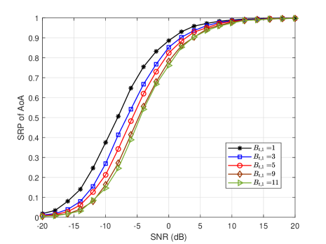
Fig. 3: SRP of AoA vs. SNR (dB) ($N_{r}=20,N_{t}=64,L=4,N=4,s=1,E_{1}=10,\widetilde{B}_{t,1}=1$).

Therefore, based on Theorem 3, the maximum SRP of AoA estimation for a given $E_{1}$ is given by

$$P_{I}\left(\frac{E_{1}N}{\widetilde{B}_{t,1}N_{r}},\widetilde{B}_{t,1}\right)=F_{2}\left(\frac{{h_{\text{min}}^{2}(1-(2L-1)\mu_{1})^{2}E_{1}N/N_{r}}-4\sigma^{2}N_{t}\mu_{{N_{r},\widetilde{B}_{t,1}}}}{4N_{t}\sigma^{2}\sigma_{{N_{r},\widetilde{B}_{t,1}}}}\right).$$ (43)

We demonstrate Theorem 3 via numerical simulations in Fig. 3, in which the SRP of AoA is evaluated for different numbers of channel uses $B_{t,1}\in\{1,3,5,9,11\}$. The simulation parameters $N_{r}=20$, $N_{t}=64$, $L=4$, $N=4$, $s=1$, $E_{1}=10$, and $\widetilde{B}_{t,1}=1$ are assumed. The curves clearly show that the highest SRP is achieved when $B_{t,1}=1$.

Now, based on Theorem 3, the solution to (38) is readily obtained as follows. In order to make SRP of AoA higher than $\eta_{1}$ in (38), we solve the inverse function in (43) with respect to $E_{1}$ and conclude that the resource allocation of Stage I should meet the following conditions:

$$E_{1}=\frac{4\sigma^{2}N_{t}N_{r}(F_{2}^{-1}(\eta_{1})\sigma_{{N_{r},\widetilde{B}_{t,1}}}+\mu_{{N_{r},\widetilde{B}_{t,1}}})}{h_{\text{min}}^{2}(1-(2L-1)\mu_{1})^{2}N},$$ (44a)

$$B_{t,1}=\widetilde{B}_{t,1},$$ (44b)

$$p_{1}=\frac{E_{1}N}{\widetilde{B}_{t,1}N_{r}},$$ (44c)

where $F_{2}^{-1}(\cdot)$ is the inverse function of $F_{2}(\cdot)$. By using similar procedures of the proof of Theorem 3, we observe the following more general result about the number of vectors $d$ in the signal model stated Lemma 1.

Corollary 1:

The bound in (30) is a monotonically decreasing function of the number of measurement vectors $d$.

Remark 7:

Corollary 1 states the effect of $d$ on the recovery performance of SOMP. It can be interpreted in the following way. The increase of the number of measurement vectors $d$ has an effect of increasing the number of columns of $\mathbf{C}$ in Lemma 1 while keeping the $C_{\min}$ unchanged. This leads to the increase of the noise power due to the increase in the dimension of $\mathbf{N}$, which in turn reduces SRP.

When it comes to the number of channel uses $B_{t,2}$ at Stage II, we cannot reach the same conclusion as Theorem 3 because the constant $\mu_{2}$ in (34) changes with $B_{t,2}$. Therefore, Given $B_{t,1}=\widetilde{B}_{t,1}$ and the total number of channel uses $K$ for channel sounding, $B_{t,2}$ is determined by (28), i.e., $K=\widetilde{B}_{t,1}{N_{r}}/{N}+B_{t,2}$. Then, the solution to (39) is given by

$$E_{2}=\frac{4\sigma^{2}N_{t}(F_{2}^{-1}(\eta_{2})\sigma_{{B_{t,2},L}}+\mu_{{B_{t,2},L}})}{h_{\text{min}}^{2}(1-(2L-1)\mu_{2})^{2}},$$ (45a)

$$B_{t,2}=K-\widetilde{B}_{t,1}{N_{r}}/{N},$$ (45b)

$$p_{2}=\frac{E_{2}}{K-\widetilde{B}_{t,1}{N_{r}}/{N}}.$$ (45c)

In summary, after solving the two-subproblems in (38) and (39), we successfully solve the problem in (37). The specific resource allocations for two stages are shown in (44c) and (45c), respectively. In particular, when the total power budget $E\geq E_{1}+E_{2}$, the joint SRP of AoA and AoD is at least $\eta_{1}\eta_{2}$.

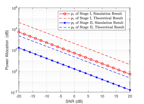
Fig. 4: Power allocation to achieve the required SRP vs. SNR (dB) ($N_{r}=20,N_{t}=64,L=4,N=4,s=1,\widetilde{B}_{t,1}=1,\eta_{1}=\eta_{2}=0.95$).

In Fig. 4, we illustrate the designed resource allocations in (44c) and (45c) with the simulation results. The parameters are set as $\eta_{1}=\eta_{2}=0.95$. The curves of theoretical results calculate the power allocations $p_{1}$ and $p_{2}$ through (44c) and (45c). The curves of simulation results are the required power allocations to achieved SRPs of $\eta_{1}$ and $\eta_{2}$. The simulation parameters $N_{r}=20$, $N_{t}=64$, $L=4$, $N=4$, $s=1$ are assumed. In Fig. 4, to achieve the same required SRP, i.e., $\eta_{1}=\eta_{2}=0.95$, Stage II requires less power allocation than Stage I. This is because the design of the sounding beams for Stage II saves the power consumption. Overall, the trend of the theoretical results is consistent with that of the simulation results, which validates the proposed resource allocation strategies in (44c) and (45c).

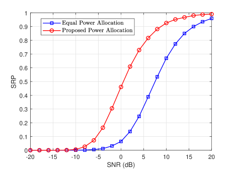
Fig. 5: Evaluation of the power allocation strategy with equal power allocation ($N_{r}=20,N_{t}=64,L=4,N=4,s=1,\widetilde{B}_{t,1}=1,\eta_{1}=\eta_{2}=0.95$).

In Fig. 5, we demonstrate the SRP of AoA and AoD achieved by the power allocations in (44c) and (45c) compared to the equal power allocation. The power allocations $p_{1}$ and $p_{2}$ are calculated by setting $\eta_{1}=\eta_{2}=0.95$ and $\sigma=0.1$ in (44c) and (45c). The simulation parameters are $N_{r}=20$, $N_{t}=64$, $L=4$, $N=4$, $s=1$. As we can see from Fig. 5, the proposed power allocation achieves much higher SRP than that of the equal power allocation, which verifies the effectiveness of the proposed power allocation strategy.

V Extension to Two-stage Method with Super Resolution

In this section, we extend the proposed two-stage method to the one with super resolution, through which we aim to address the issue of unresolvable quantization errors. Among the existing works, there are two directions to solve the quantization error for off-grid effect. Firstly, the works in [46, 47, 48] model the response vector as the summation of on-grid part and the approximation error, in which the sparse Bayesian inference is utilized to estimate the approximation error. Secondly, the atomic norm minimization has been proposed in [19, 20, 21], which can be viewed as the case when the infinite dictionary matrix is employed. Based on atomic norm minimization, the sparse signal recovery is reformulated as a semidefinite programming. Compared to the sparse Bayesian inference, one advantage of atomic norm minimization is that the recovery guarantee is analyzable [19, 20, 21]. Following the methodology of the atomic norm minimization, in this section, we aim to estimate the AoAs and AoDs, i.e., $\{f_{r,1},\ldots,f_{r,L}\}$ and $\{f_{t,1},\ldots,f_{t,L}\}$, under the proposed two-stage framework.

V-A Super Resolution AoA Estimation

The sounding beams of Stage I, i.e., $\mathbf{F}_{b,1}$ and $\mathbf{W}_{b,1}$, are designed according to (15) and (18). By using the exact expression of $\mathbf{H}$ in (2) rather than the quantized version in (8), the observations for Stage I is given by

$$\mathbf{Y}_{1} =\mathbf{W}_{b,1}^{H}\mathbf{H}\mathbf{F}_{b,1}+\mathbf{W}_{b,1}^{H}\mathbf{N}_{1}$$

$$=\mathbf{W}_{b,1}^{H}{{\mathbf{A}}_{r}}\operatorname{diag}(\mathbf{h})\mathbf{A}_{t}^{H}{\mathbf{F}_{b,1}}+\mathbf{W}_{b,1}^{H}\mathbf{N}_{1}$$

$$=\mathbf{W}_{b,1}^{H}{{\mathbf{A}}_{r}}{{\mathbf{C}}_{r}}+\mathbf{W}_{b,1}^{H}\mathbf{N}_{1},$$ (46)

where $\mathbf{Y}_{1}\in{\mathbb{C}}^{N_{r}\times B_{t,1}}$ and $\mathbf{C}_{r}=\operatorname{diag}(\mathbf{h})\mathbf{A}_{t}^{H}{\mathbf{F}_{b,1}}\in{\mathbb{C}}^{L\times B_{t,1}}$. Since $\mathbf{W}_{b,1}=\mathbf{S}_{N_{r}}$ in (18), projecting $\mathbf{Y}_{1}$ onto $\mathbf{W}_{b,1}$ yields

$$\widetilde{\mathbf{Y}}_{1}=\mathbf{W}_{b,1}\mathbf{Y}_{1}={{\mathbf{A}}_{r}}{{\mathbf{C}}_{r}}+\mathbf{N}_{1}.$$ (47)

The observation in (47) is rewritten by explicitly involving the array response vectors,

$$\widetilde{\mathbf{Y}}_{1}=[{\mathbf{a}_{r}}({{f}_{r,1}}),\ldots,{\mathbf{a}_{r}}({{f}_{r,L}})]{{\mathbf{C}}_{r}}+\mathbf{N}_{1}=\mathbf{R}_{1}+\mathbf{N}_{1},$$ (48)

where $\mathbf{R}_{1}=[{\mathbf{a}_{r}}({{f}_{r,1}}),\ldots,{\mathbf{a}_{r}}({{f}_{r,L}})]{{\mathbf{C}}_{r}}\in{\mathbb{C}}^{N_{r}\times B_{t,1}}$. The atom ${{\mathbf{A}}_{r}}(f,\mathbf{b})\in{\mathbf{C}^{N_{r}\times B_{t,1}}}$ is defined in [20, 19] as ${{\mathbf{A}}_{r}}(f,\mathbf{b})={\mathbf{a}_{r}}(f){{\mathbf{b}}^{H}}$, where $f\in[0,1)$ and $\mathbf{b}\in{\mathbb{C}}^{B_{t,1}\times 1}$ with ${{\left\|\mathbf{b}\right\|}_{2}}=1$. We let the collection of all such atoms be the set $\mathcal{A}_{r}=\{{{\mathbf{A}}_{r}}(f,\mathbf{b}):f\in[0,1),{{\left\|\mathbf{b}\right\|}_{2}}=1\}$. Obviously, the cardinality of $\mathcal{A}_{r}$ is infinite. The matrix ${{\mathbf{R}}_{1}}$ in (48) can be written as the linear combination among the atoms from the atomic set ${{\mathcal{A}}_{r}}$,

$${{\mathbf{R}}_{1}}=\sum\limits_{l=1}^{L}{{{[\mathbf{c}_{r}]}_{l}}{{\mathbf{A}}_{r}}({{f}_{r,l}},{{\mathbf{b}}_{l}})}=\sum\limits_{l=1}^{L}{{{[\mathbf{c}_{r}]}_{l}}{\mathbf{a}_{r}}({{f}_{r,l}})}\mathbf{b}_{l}^{H},$$ (49)

where $\mathbf{c}_{r}\in{\mathbb{R}}^{L\times 1}$ is the coefficient vector with $[\mathbf{c}_{r}]_{l}\geq 0$, and it has the relationship $[\mathbf{C}_{r}]_{l,:}=[\mathbf{c}_{r}]_{l}\mathbf{b}_{l}^{H},~{}\forall\,l=1,\ldots,L$. Observing (49), the dimension of vector $\mathbf{c}_{r}$, i.e., $L$, can be interpreted as the sparest representation of $\mathbf{R}_{1}$ in the context of the atomic set ${\mathcal{A}}_{r}$. Therefore, in order to seek the sparsest representation, after taking the noise in (48) into account, the reconstruction problem is formulated by

$$\underset{\mathbf{R}_{1}}{\mathop{\min}}\,{\left\|\mathbf{R}_{1}\right\|}_{\mathcal{A}_{r},0}+\frac{\lambda_{1}}{2}\|\widetilde{\mathbf{Y}}_{1}-\mathbf{R}_{1}\|_{F}^{2},$$ (50)

where $\lambda_{1}>0$ is the penalty parameter, and ${\left\|{{\mathbf{R}}_{1}}\right\|}_{{{\mathcal{A}}_{r}},0}$ is defined as

$${{\left\|{{\mathbf{R}}_{1}}\right\|}_{{{\mathcal{A}}_{r}},0}} =\underset{\mathbf{c}_{r}}{\mathop{\inf}}\,{{\left\|\mathbf{c}_{r}\right\|}_{0}}$$ (51a)

subject to $${{\mathbf{R}}_{1}}=\sum\limits_{l=1}^{L}{{{[\mathbf{c}_{r}]}_{l}}{{\mathbf{A}}_{r}}({{f}_{r,l}},{{\mathbf{b}}_{l}})},$$ (51b)

$$\text{ }{{\mathbf{A}}_{r}}({{f}_{r,l}},{{\mathbf{b}}_{l}})\in{{\mathcal{A}}_{r}},{{[\mathbf{c}_{r}]}_{l}}\geq 0,$$ (51c)

with $\|\mathbf{R}_{1}\|_{{\mathcal{A}}_{r},0}$ revealing the minimal number of atoms in $\mathbf{R}_{1}$. When the sparest representation of $\mathbf{R}_{1}$, i.e., $\{{{{[\mathbf{c}_{r}]}_{l}}{\mathbf{a}_{r}}({{f}_{r,l}})}\mathbf{b}_{l}^{H}\}_{l=1}^{L}$, is found by solving (50), the AoAs $\{f_{r,l}\}_{l=1}^{L}$ can be obtained from the atomic decomposition in (49). However, since the minimization problem in (51) is combinatorial, it is not tractable to calculate the value of ${{\left\|{{\mathbf{R}}_{1}}\right\|}_{{{\mathcal{A}}_{r}},0}}$. To overcome the challenge, the problem in (50) is relaxed as,

$$\underset{\mathbf{R}_{1}}{\mathop{\min}}\,{\left\|\mathbf{R}_{1}\right\|}_{\mathcal{A}_{r},1}+\frac{\lambda_{1}}{2}\|\widetilde{\mathbf{Y}}_{1}-\mathbf{R}_{1}\|_{F}^{2},$$ (52)

where ${{\left\|{{\mathbf{R}}_{1}}\right\|}_{{{\mathcal{A}}_{r}},1}}$ is the atomic norm of $\mathbf{R}_{1}$ defined by

$${{\left\|{{\mathbf{R}}_{1}}\right\|}_{{{\mathcal{A}}_{r}},1}} =\underset{\mathbf{c}_{r}}{\mathop{\inf}}\,{{\left\|\mathbf{c}_{r}\right\|}_{1}}$$ (53a)

subject to $${{\mathbf{R}}_{1}}=\sum\limits_{l=1}^{L}{{{[\mathbf{c}_{r}]}_{l}}{{\mathbf{A}}_{r}}({{f}_{r,l}},{{\mathbf{b}}_{l}})},$$ (53b)

$$\text{ }{{\mathbf{A}}_{r}}({{f}_{r,l}},{{\mathbf{b}}_{l}})\in{{\mathcal{A}}_{r}},{{[\mathbf{c}_{r}]}_{l}}\geq 0.$$ (53c)

It is noted that in (53), the atomic norm $\|\mathbf{R}_{1}\|_{{\mathcal{A}}_{r},1}$ is to minimize the summation of entries in $\mathbf{c}_{r}$ instead of the number of non-zero elements in (51).

Different from the intractability of (51), the problem in (53) can be efficiently solved by semi-definite programming [19]:

$${{\left\|{{\mathbf{R}}_{1}}\right\|}_{{{\mathcal{A}}_{r}},\text{1}}}=\underset{\mathbf{u},\mathbf{Z}}{\mathop{\inf}}\,\frac{1}{2}\text{tr}\left(\text{Toeplitz}(\mathbf{u})\right)+\frac{1}{2}\text{tr}(\mathbf{Z})$$ (54a)

$$\text{subject to }\left[\begin{matrix}\text{Toeplitz}(\mathbf{u})&{{\mathbf{R}}_{1}}\\ \mathbf{R}_{1}^{H}&\mathbf{Z}\\ \end{matrix}\right]\succeq\mathbf{0},$$ (54b)

where $\mathbf{u}\in{\mathbf{C}^{N_{r}\times 1}},\mathbf{Z}\in{\mathbf{C}^{B_{t,1}\times B_{t,1}}}$, and $\text{Toeplitz}(\mathbf{u})\in{\mathbf{C}^{N_{r}\times N_{r}}}$ denotes the Hermitian Toeplitz matrix generated by the vector $\mathbb{u}$. Plugging (54) into (52) gives

$$\underset{\mathbf{u},\mathbf{Z},\mathbf{R}_{1}}{\mathop{\inf}}~{}\text{tr}\left(\text{Toeplitz}(\mathbf{u})\right)+\text{tr}(\mathbf{Z})+{\lambda_{1}}\|\widetilde{\mathbf{Y}}_{1}-\mathbf{R}_{1}\|_{F}^{2}$$ (55a)

$$\text{subject to }\mathbf{X}=\left[\begin{matrix}\text{Toeplitz}(\mathbf{u})&{{\mathbf{R}}_{1}}\\ \mathbf{R}_{1}^{H}&\mathbf{Z}\\ \end{matrix}\right],~{}\mathbf{X}\succeq\mathbf{0}.$$ (55b)

It is straightforward to find that (55) is convex, where ADMM can be employed to accelerate the computation. The augmented Lagrangian of (55) is expressed as

$$\mathcal{L}(\mathbf{u},\mathbf{Z},\mathbf{R}_{1},\mathbf{X},\bm{\Lambda}) =\text{tr}\left(\text{Toeplitz}(\mathbf{u})\right)+\text{tr}(\mathbf{Z})+{\lambda_{1}}\|\widetilde{\mathbf{Y}}_{1}-\mathbf{R}_{1}\|_{F}^{2}$$

$$~{}~{}+\left<\bm{\Lambda},\mathbf{X}-\left[\begin{matrix}\text{Toeplitz}(\mathbf{u})&{{\mathbf{R}}_{1}}\\ \mathbf{R}_{1}^{H}&\mathbf{Z}\\ \end{matrix}\right]\right>+\frac{\rho}{2}\left\|\mathbf{X}-\left[\begin{matrix}\text{Toeplitz}(\mathbf{u})&{{\mathbf{R}}_{1}}\\ \mathbf{R}_{1}^{H}&\mathbf{Z}\\ \end{matrix}\right]\right\|_{F}^{2},$$ (56)

where $\mathbf{X}\in{\mathbb{C}}^{(N_{r}+B_{t,1})\times(N_{r}+B_{t,1})}$ and $\bm{\Lambda}\in{\mathbb{C}}^{(N_{r}+B_{t,1})\times(N_{r}+B_{t,1})}$ are Hermitian matrices, and $\rho$ is the Lagrangian multiplier. Then, with $t$ being the iteration index, we iteratively update the variables in (56) as follows:

$$(\mathbf{u}^{t+1},\mathbf{Z}^{t+1},\mathbf{R}_{1}^{t+1}) =\operatorname*{arg\,min}_{\mathbf{u},\mathbf{Z},\mathbf{R}_{1}}\mathcal{L}(\mathbf{u},\mathbf{Z},\mathbf{R}_{1},\mathbf{X}^{t},\bm{\Lambda}^{t}),$$ (57)

$$\mathbf{X}^{t+1} =\operatorname*{arg\,min}_{\mathbf{X}\succeq\mathbf{0}}\mathcal{L}(\mathbf{u}^{t+1},\mathbf{Z}^{t+1},\mathbf{R}_{1}^{t+1},\mathbf{X},\bm{\Lambda}^{t}),$$ (58)

$$\bm{\Lambda}^{t+1} =\bm{\Lambda}^{t}+\rho\left(\mathbf{X}^{t+1}-\left[\begin{matrix}\text{Toeplitz}(\mathbf{u}^{t+1})&{{\mathbf{R}}_{1}^{t+1}}\\ (\mathbf{R}^{t+1}_{1})^{H}&\mathbf{Z}^{t+1}\end{matrix}\right]\right).$$ (59)

The solutions of the (57) and (58) are respectively

$$[\mathbf{u}^{t+1}]_{i} =\begin{cases}\frac{V_{i}+\rho S_{i}}{(N_{r}-t)\rho+N_{r}},&i=1\\ \frac{V_{i}+\rho S_{i}}{(N_{r}-t)\rho},&i=2,\ldots,N_{r}\end{cases},\text{with }V_{i}=\sum_{k=1}^{N_{r}+1-i}[\bm{\Lambda}^{t}]_{k,k-1+i},~{}S_{i}=\sum_{k=1}^{N_{r}+1-i}[\mathbf{X}^{t}]_{k,k-1+i},$$

$$\mathbf{R}_{1}^{t+1} =\frac{1}{\lambda_{1}+\rho}(\lambda_{1}\widetilde{\mathbf{Y}}_{1}+\rho[\mathbf{X}^{t}]_{1:N_{r},N_{r}+1:\text{end}}+[\bm{\Lambda}^{t}]_{1:N_{r},N_{r}+1:\text{end}}),$$

$$\mathbf{Z}^{t+1} =\frac{1}{\rho}([\bm{\Lambda}^{t}]_{N_{r}+1:\text{end},N_{r}+1:\text{end}}+\rho[\mathbf{X}^{t}]_{N_{r}+1:\text{end},N_{r}+1:\text{end}}-\mathbf{I}_{B_{t,1}}),$$

$$\mathbf{X}^{t+1} =\left[\begin{matrix}\text{Toeplitz}(\mathbf{u}^{t+1})&{{\mathbf{R}}_{1}^{t+1}}\\ (\mathbf{R}^{t+1}_{1})^{H}&\mathbf{Z}^{t+1}\\ \end{matrix}\right]-\frac{1}{\rho}\bm{\Lambda}^{t}.$$

It is worth noting that in order to guarantee $\mathbf{X}\succeq 0$ as shown in (58), we can set the negative eigenvalues of $\mathbf{X}^{t+1}$ to $0$. When the iterative process converges, the result $\text{Toeplitz}(\mathbf{u})$ can be utilized to obtain the estimation of AoAs. Specifically, we can take Vandermonde decomposition [19] for $\text{Toeplitz}(\mathbf{u})$, $\text{Toeplitz}(\mathbf{u})=\mathbf{V}\mathbf{D}\mathbf{V}^{H}$, where $\mathbf{V}=[\mathbf{a}_{r}(\hat{f}_{r,1}),\ldots,\mathbf{a}_{r}(\hat{f}_{r,L})]\in{\mathbb{C}}^{N_{r}\times L}$ with $\{\hat{f}_{r,l}\}_{l=1}^{L}$ being the estimated AoAs and $\mathbf{D}=\operatorname{diag}([d_{1},\ldots,d_{L}])\in{\mathbb{C}}^{L\times L}$. In practice, it is not necessary to calculate the Vandermonde decomposition of $\text{Toeplitz}(\mathbf{u})$ explicitly. Since the column subspace of $\text{Toeplitz}(\mathbf{u})$ is equal to ${\mathcal{R}}(\mathbf{V})$, the set of AoAs can be estimated from $\text{Toeplitz}(\mathbf{u})$ efficiently by spectrum estimation algorithms such as MUSIC or ESPRIT [20, 19].

V-B Super Resolution AoD Estimation

Similarly, the observations for the second stage is given by

$$\mathbf{Y}_{2} =\mathbf{W}_{b,2}^{H}\mathbf{H}\mathbf{F}_{b,2}+\mathbf{W}_{b,2}^{H}\mathbf{N}_{2}$$

$$=\mathbf{W}_{b,2}^{H}{{\mathbf{A}}_{r}}\operatorname{diag}(\mathbf{h})\mathbf{A}_{t}^{H}\mathbf{F}_{b,2}+\mathbf{W}_{2}^{H}\mathbf{N}_{2}$$

$$=\mathbf{C}_{t}\mathbf{A}_{t}^{H}\mathbf{F}_{b,2}+\mathbf{W}_{b,2}^{H}\mathbf{N}_{2},$$ (60)

where we let $\mathbf{C}_{t}=\mathbf{W}_{b,2}^{H}{{\mathbf{A}}_{r}}\operatorname{diag}(\mathbf{h})\in{\mathbb{C}}^{L\times L}$. At Stage II, the observation $\mathbf{Y}_{2}$ in (60) is rewritten as

$$\mathbf{Y}_{2}^{H}=\mathbf{F}_{b,2}^{H}\mathbf{A}_{t}\mathbf{C}_{t}^{H}+\mathbf{N}_{2}^{H}\mathbf{W}_{b,2}=\mathbf{R}_{2}^{H}+\mathbf{N}_{2}^{H}\mathbf{W}_{b,2},$$ (61)

where we let $\mathbf{R}_{2}=\mathbf{F}_{b,2}^{H}\mathbf{A}_{t}\mathbf{C}_{t}^{H}\in{\mathbb{C}}^{B_{t,2}\times L}$. Due to the design of $\mathbf{F}_{b,2}$ in (27), we have

$$\mathbf{F}_{b,2}^{H}\mathbf{A}_{t}=\sqrt{p_{2}}[\mathbf{A}_{t}]_{1:B_{t,2},:}=\sqrt{p_{2}}[\mathbf{a}_{t}({{f}_{t,1}}),\ldots,\mathbf{a}_{t}({{f}_{t,L}})]_{1:B_{t,2},:}.$$

For convenience, we define $\widetilde{\mathbf{a}}_{t}(f)=[\mathbf{a}_{t}(f)]_{1:B_{t,2}}\in{\mathbb{C}}^{B_{t,2}\times 1}$ and $\widetilde{\mathbf{A}}_{t}=[\widetilde{\mathbf{a}}_{t}({{f}_{t,1}}),\ldots,\widetilde{\mathbf{a}}_{t}({{f}_{t,L}})]\in{\mathbb{C}}^{B_{t,2}\times L}$. The AoD estimation boils down to extracting $L$ parameters $\left\{{{f}_{t,l}}\right\}_{l=1}^{L}$ in $\widetilde{\mathbf{A}}_{t}$. We let ${{\mathbf{A}}_{t}}(f,\mathbf{b})\in{\mathbf{C}^{B_{t,2}\times L}}$ be ${\mathbf{A}_{t}}(f,\mathbf{b})={\widetilde{\mathbf{a}}_{t}}(f){{\mathbf{b}}^{H}}$, where $f\in[0,1)$, $\mathbf{b}\in{\mathbb{C}}^{L\times 1}$ with ${{\left\|\mathbf{b}\right\|}_{2}}=1$, and the atomic set ${\mathcal{A}}_{t}$ is defined by $\mathcal{A}{{}_{t}}=\{{{\mathbf{A}}_{t}}(f,\mathbf{b}):f\in[0,1],{{\left\|\mathbf{b}\right\|}_{2}}=1\}$, Similarly, ${\mathbf{R}}_{2}^{H}$ in (61) can be written as the linear combination of the atoms from the set ${\mathcal{A}}_{t}$,

$${\mathbf{R}}_{2}^{H}=\sum\limits_{l=1}^{L}{{[\mathbf{c}_{t}]}_{l}}{{\mathbf{A}}_{t}}({{f}_{t,l}},{{\mathbf{b}}_{l}})=\sum\limits_{l=1}^{L}{{{[\mathbf{c}_{t}]}_{l}}{\mathbf{a}_{t}}({{f}_{t,l}})}\mathbf{b}_{l}^{H},$$

where $\mathbf{c}_{t}\in{\mathbb{R}}^{L\times 1}$ is the coefficient vector with $[\mathbf{c}_{t}]_{l}\geq 0$. Therefore, using the similar approach as AoA estimation in (52), the AoD estimation problem is given by

$$\underset{\mathbf{R}_{2}}{\mathop{\min}}\,{\left\|\mathbf{R}_{2}^{H}\right\|}_{\mathcal{A}_{t},1}+\frac{\lambda_{2}}{2}\left\|\mathbf{Y}_{2}-\mathbf{R}_{2}\right\|_{F}^{2},$$ (62)

where $\lambda_{2}$ is a penalty parameter. The problem in (62) can also be solved in a similar manner as (52), and the estimation for AoDs, i.e., $\{\hat{f}_{t,l}\}_{l=1}^{L}$, can be obtained.

Furthermore, after the AoAs $\{\hat{f}_{r,l}\}_{l=1}^{L}$ and AoDs $\{\hat{f}_{t,l}\}_{l=1}^{L}$ are estimated, we can easily calculate the AoA and AoD array response matrix $\widehat{\mathbf{A}}_{r}$ and $\widehat{\mathbf{A}}_{t}$. Then, by using the channel estimation technique provided in Section III-C, the final channel estimation result is obtained.

VI Simulation Results

In this section, we evaluate the performance of the proposed two-stage AoA and AoD estimation method and two-stage method with super resolution. For comparison, we take the OMP-based mmWave channel estimation method [9] as our benchmark. Also, we include the oracle estimator as we discussed in (7). The parameter settings for evaluation are as follows. We assume throughout the simulation $N_{r}=20,N_{t}=64$, and the channel model is given by (1). We let the dimensions of the angle grids for the proposed two-stage method and OMP [9] be $G_{r}=sN_{r}$ and $G_{t}=sN_{t}$. The number of paths is $L=4$. The variance of the path gain is $\sigma_{l}^{2}=1,\forall\,l$. The number of RF chains is $N=4$. The number of channel uses for the estimation task is $K=50$. The minimum allowed transmit beams at Stage I are $\widetilde{B}_{t,1}=1$. Without loss of generality, for the proposed two-stage framework, the power budget $E=E_{1}+E_{2}$, where $E_{1}$ and $E_{2}$ are, respectively, given by the resource allocations in (44c) and (45c) with $\eta_{1}=\eta_{2}=0.95$ and SNR$=20$dB.

To evaluate the estimation performance, we use three performance metrics:

• The first metric is the SRP. The error of the estimated angles are defined as

  $$\epsilon=\frac{1}{2L}\sum_{l=1}^{L}\left(|f_{r,l}-\hat{f}_{r,l}|^{2}+|f_{t,l}-\hat{f}_{t,l}|^{2}\right).$$

  We declare the reconstruction is successful if $\epsilon\leq 10^{-3}$. Precisely, SRP is defined as

  $$\text{SRP}=\frac{\text{number of trials with }\epsilon\leq 10^{-3}}{\text{number of total trials}}.$$

• The second metric is MSE of angle estimation defined as

  $$\text{MSE}={\mathbb{E}}\left[\sum_{l=1}^{L}\left(|f_{r,l}-\hat{f}_{r,l}|^{2}+|f_{t,l}-\hat{f}_{t,l}|^{2}\right)\right].$$

• The third metric is NMSE of channel estimation defined as

  $$\text{NMSE}={\mathbb{E}}[\|\mathbf{H}-\widehat{\mathbf{H}}\|_{F}^{2}/\|\mathbf{H}\|_{F}^{2}],$$

  where $\widehat{\mathbf{H}}$ is the channel estimate.

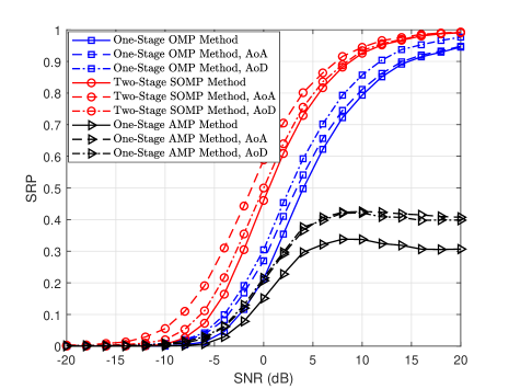
Fig. 6: SRP vs. SNR (dB) with discrete angles ($N_{r}=20,N_{t}=64,L=4,N=4,K=50,\widetilde{B}_{t,1}=1,s=1$).

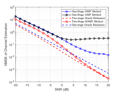
Fig. 7: NMSE vs. SNR (dB) with discrete angles ($N_{r}=20,N_{t}=64,L=4,N=4,K=50,\widetilde{B}_{t,1}=1,s=1$).

VI-A Channel Estimation Performance of Two-stage Method with Discrete Angles

For the simulations with discrete angles in Figs. 6-7, the ${{f}_{t,l}}$ and $f_{r,l}$ in (1) are uniformly distributed on the grids of size $G_{t}=N_{t}$ and $G_{r}=N_{r}$, respectively. Three methods are compared, which are proposed two-stage SOMP method, one-stage OMP method [9], AMP method [49], and oracle method in (7). We show the SRP in Fig. 6 and NMSE in Fig. 7.

In Fig. 6, considering that oracle method assumes that AoAs and AoDs are known as a priori, we do not illustrate the performance of the oracle method when comparing the SRP. As can be seen in Fig. 6, the proposed two-stage SOMP method achieves a higher SRP compared to the benchmarks. It is worth noting that the AMP-based method require the minimal measurements to guarantee the convergence [49]. When the number of channel uses is limited, the AMP-based method can not achieve the near one SRP even if the SNR is high. Also, the SRPs of AoA and AoD of the proposed two-stage SOMP method are both higher than those of one-stage OMP method. The improvement of SRP of AoD is because we optimize the sounding beams of the second stage based on the estimated AoA result. For the improvement of SRP of AoA, it is because we allocate more power budget to Stage I according to the proposed resource allocation strategy.

Similarly, in Fig. 7, the proposed two-stage SOMP method has lower NMSE than the one-stage OMP and AMP methods. In addition, we can find from Fig. 7 that the proposed two-stage SOMP method converges to the performance of the oracle method as SNR grows. Overall, Figs. 6-7 verify that the proposed two-stage method outperforms the one-stage OMP in the scenario of discrete angles.

VI-B Channel Estimation Performance of Two-stage Method with Continuous Angles

For this set of simulations in Fig. 8-9, we assume the ${{f}_{t,l}}$ and $f_{r,l}$ in (1) are uniformly distributed in $[0,1)$. Four methods are compared, which are the proposed two-stage SOMP method, two-stage method with super resolution, one-stage OMP method [9], and one-stage atomic method [21]. When implementing the two-stage SOMP method and one-stage OMP method with the defined angle grids, the estimated angles are located on the defined grids. Fig. 8 illustrates the MSE and Fig. 9 illustrates the NMSE of channel estimation.

In Fig. 8, the proposed two-stage SOMP method and two-stage method with super resolution outperform the one-stage OMP and one-stage atomic method, respectively. Interestingly, the two-stage SOMP method achieves the minimal MSE when SNR is low. This is because when SNR is low, i.e., $\text{SNR}\leq 5\text{dB}$, the noise power is higher than that of the quantization error. Therefore, using the quantized model could reduce the complexity of problem and achieve near-optimal performance. When SNR is high, i.e., $\text{SNR}\geq 5\text{dB}$, the two-stage method with super resolution achieves the minimal MSE. This is because when SNR is high, the quantization error will become dominant, which can not be handled by the grid-based methods. Nevertheless, the Fig. 8 verifies that by dividing the estimation into two stages, the estimation of AoAs and AoDs is improved compared to the one-stage estimation.

Likewise, in Fig. 9, the proposed two-stage SOMP method and two-stage method with super resolution also achieve lower NMSE than the one-stage OMP and one-stage atomic methods. Similarly, when SNR is high, the two-stage method with super resolution shows the minimum NMSE.

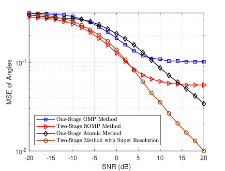
Fig. 8: MSE vs. SNR (dB) with continuous angles ($N_{r}=20,N_{t}=64,L=4,N=4,K=50,\widetilde{B}_{t,1}=1,s=2$).

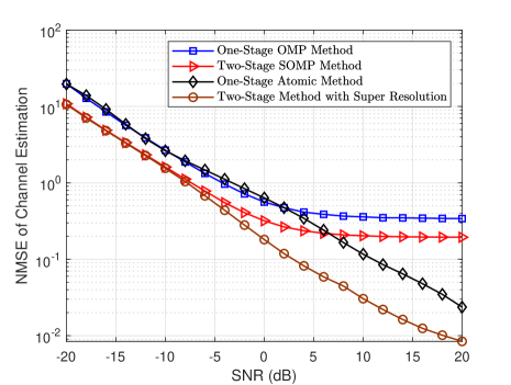
Fig. 9: NMSE vs. SNR (dB) with continuous angles ($N_{r}=20,N_{t}=64,L=4,N=4,K=50,\widetilde{B}_{t,1}=1,s=2$).

VI-C Analysis of Computational Complexity

For two-stage method, the computational complexity for the first stage is $\mathcal{O}(LN_{r}G_{r})=\mathcal{O}(sLN_{r}^{2})$, and the complexity for the second stage is $\mathcal{O}(LB_{t,2}G_{t})=\mathcal{O}(sL(K-N_{r}/N)N_{t})=\mathcal{O}(sLKN_{t})$ with $K$ being the number of channel uses. Therefore, the total computational complexity for two-stage method is $\mathcal{O}(sLN_{r}^{2})+\mathcal{O}(sLKN_{t})=\mathcal{O}(sLKN_{t})$. However, for the one-stage OMP method, the computational complexity is $\mathcal{O}(LKNG_{t}G_{r})=\mathcal{O}(s^{2}LKNN_{t}N_{r})$. It is obvious that the two-stage method has much lower computational complexity compared to the one-stage OMP by $\mathcal{O}(sNN_{r})$ times.

For the two-stage method with super resolution, in Stage I, the computational complexity of ADMM per iteration is dominated by the eigenvalue decomposition of $\mathbf{X}^{t+1}$, i.e., $\mathcal{O}(N_{r}^{3})$. Similarly, for Stage II, each iteration has the computational complexity of $\mathcal{O}(B_{t,2}^{3})=\mathcal{O}((K-N_{r}/N)^{3})=\mathcal{O}(K^{3})$. Given the number of iteration $T$ and $K\geq N_{r}$, the total computational complexity of the super resolution method is $\mathcal{O}(TN_{r}^{3})+\mathcal{O}(TK^{3})=\mathcal{O}(TK^{3})$. In order to compare the complexities of the two-stage method with super resolution and one-stage OMP, we consider a simple example as follows. In particular, if $N_{r}=N_{t}$ and $K=\mathcal{O}(N_{r})$, the complexity of the proposed two-stage method with super resolution is $\mathcal{O}(s^{2}LN/T)$ times lower than that of the one-stage OMP.

VII Conclusion

In this paper, the two-stage method for the mmWave channel estimation was proposed. By sequentially estimating AoAs and AoDs of large-dimensional antenna arrays, the proposed two-stage method saved the computational complexity as well as channel use overhead compared to the existing methods. Theoretically, we analyzed the SRPs of AoA and AoD of the proposed two-stage method. Based on the analyzed SRP, we designed the resource allocation strategy among two stages to guarantee the accurate AoA and AoD estimation. In addition, to resolve the issue of quantization error, we extended the proposed two-stage method to a version with super resolution. The numerical simulations showed that the proposed two-stage method achieves more accurate channel estimation result than the one-stage method.

Appendix A Proof of Lemma 1

For an arbitrary random noise matrix $\mathbf{N}$, the SRP of SOMP has been characterized in [33]. This result is general to be extended to the case in Lemma 1, where the entries in $\mathbf{N}$ are i.i.d. complex Gaussian.

Theorem 4:

(SRP of SOMP with arbitrary random noise [33]) Suppose the signal model provided in Lemma 1. Given the measurement matrix $\bm{\Phi}$ with its MIP constant satisfying $\mu<1/(2L+1)$ and the cumulative distribution function (CDF) of $\|\mathbf{N}\|_{2}$ satisfying

$$\text{Pr}(\|\mathbf{N}\|_{2}\leq x)=F_{N}(x),$$ (63)

the SRP of SOMP in Algorithm 1 satisfies

$$\text{Pr}({\mathcal{V}}_{S})\geq F_{N}\left(\frac{C_{\text{min}}{{(1-(2L-1)\mu)}}}{2}\right),$$ (64)

where ${\mathcal{V}}_{S}$ is the event of successful reconstruction of Algorithm 1, $C_{\min}=\min\limits_{i\in\Omega}\left\|[\mathbf{C}]_{i,:}\right\|_{2}$.

According to the results in Theorem 4, the SRP of SOMP is characterized by the CDF of $\|\mathbf{N}\|_{2}$. Thus, in order to extend the result provided in Theorem 4 to the case in Lemma 1, the CDF of $\|\mathbf{N}\|_{2}$ is of interest when the entries of $\mathbf{N}\in{\mathbb{C}}^{M\times d}$ are i.i.d. ${\mathcal{C}}{\mathcal{N}}(0,\sigma^{2})$. Fortunately, according to [41, 40], the CDF of the largest singular value of $\mathbf{N}$ converges in distribution to the Tracy-Widom law as $M,d$ tend to $\infty$,

$$\text{Pr}(\|\mathbf{N}\|_{2}\leq x)\approx F_{2}\left(\frac{{x^{2}}/{\sigma^{2}}-\mu_{M,d}}{\sigma_{M,d}}\right),$$ (65)

where the function $F_{2}(\cdot)$ is the CDF of Tracy-Widom law [41, 40], $\mu_{M,d}=(M^{1/2}+d^{1/2})^{2}$, and $\sigma_{M,d}=(M^{1/2}+d^{1/2})(M^{-1/2}+d^{-1/2})^{1/3}$. Finally, after plugging the expression in (65) into (64) of Theorem 4, we obtain Lemma 1, which completes the proof. ∎

Appendix B Proof of Proposition 2

One can write the effective noise as $\tilde{\mathbf{N}}=\mathbf{E}+\mathbf{N}$ where the entries in $\mathbf{N}$ are i.i.d. with ${\mathcal{C}}{\mathcal{N}}(0,\sigma^{2})$. Therefore, we have the following probability bound,

$$\Pr\left(\|{\tilde{\mathbf{N}}}\|_{2}\leq x\right) \overset{(a)}{\leq}\Pr\left(\left\|{\mathbf{E}}\right\|_{2}+\left\|{\mathbf{N}}\right\|_{2}\leq x\right)$$

$$\overset{(b)}{\approx}F_{2}\left(\frac{{(x-\|\mathbf{E}\|_{2})^{2}}/{{\sigma}^{2}}-\mu_{M,d}}{\sigma_{M,d}}\right),$$ (66)

where the inequality $(a)$ is due to the triangular inequality, and the approximation $(b)$ holds from (65). Then, according to Theorem 4, plugging the expression (66) into (64) leads to

$$\text{Pr}({\mathcal{V}}_{S})\geq F_{2}\left(\frac{{\left((1-(2L-1)\mu)C_{\text{min}}-2\|\mathbf{E}\|_{2}\right)^{2}}-4\sigma^{2}\mu_{M,d}}{4\sigma^{2}\sigma_{M,d}}\right),$$

where $C_{\min}=\min\limits_{i\in\Omega}\left\|[\mathbf{C}]_{i,:}\right\|_{2}$. This concludes the proof. ∎

Appendix C Proof of Theorem 2

Plugging RSB in (25) and TSB in (27) into (21) gives $\|[\bm{\Phi}_{2}]_{:,j}\|_{2}=\sqrt{{p_{2}B_{t,2}}/{N_{t}}},~{}j=1,\ldots,G_{t}$, and $C_{\min}=\min_{t_{l}\in\Omega_{t}}\|[\mathbf{C}_{2}]_{t_{l},:}\|_{2}=|{{h}_{\min}}|$ with ${{t}_{l}}$ being the index of the $l$th path of $\mathbf{A}_{t}$ in $\bar{\mathbf{A}}_{t}$ such that $[\bar{\mathbf{A}}_{t}]_{:,t_{l}}=[\mathbf{A}_{t}]_{:,l}$, $l=1,\ldots,L$. Hence, incorporating the latter $C_{\min}$ and $\|[\bm{\Phi}_{2}]_{:,j}\|_{2}$ into Lemma 1 concludes the proof. ∎

References

- [1] O. El Ayach, S. Rajagopal, S. Abu-Surra, Z. Pi, and R. W. Heath, “Spatially sparse precoding in millimeter wave MIMO systems,” IEEE Trans. Wireless Commun., vol. 13, no. 3, pp. 1499–1513, 2014.
- [2] R. W. Heath, N. González-Prelcic, S. Rangan, W. Roh, and A. M. Sayeed, “An overview of signal processing techniques for millimeter wave MIMO systems,” IEEE J. Sel. Top. Signal Process., vol. 10, no. 3, pp. 436–453, April 2016.
- [3] S. Hur, T. Kim, D. J. Love, J. V. Krogmeier, T. A. Thomas, and A. Ghosh, “Millimeter wave beamforming for wireless backhaul and access in small cell networks,” IEEE Trans. Commun., vol. 61, no. 10, pp. 4391–4403, 2013.
- [4] W. Zhang, T. Kim, D. J. Love, and E. Perrins, “Leveraging the restricted isometry property: Improved low-rank subspace decomposition for hybrid millimeter-wave systems,” IEEE Trans. Commun., vol. 66, no. 11, pp. 5814–5827, Nov 2018.
- [5] W. Zhang, T. Kim, and S. Leung, “A sequential subspace method for millimeter wave MIMO channel estimation,” IEEE Trans. Veh. Technol., vol. 69, no. 5, pp. 5355–5368, 2020.
- [6] 5GCM White Paper, “White paper on ’5G channel model for bands up to 100 GHz’,” vol. 2, March 2016.
- [7] S. Hur, S. Baek, B. Kim, Y. Chang, A. F. Molisch, T. S. Rappaport, K. Haneda, and J. Park, “Proposal on millimeter-wave channel modeling for 5G cellular system,” IEEE J. Sel. Top. Signal Process., vol. 10, no. 3, pp. 454–469, April 2016.
- [8] A. Alkhateeb, O. El Ayach, G. Leus, and R. W. Heath, “Channel estimation and hybrid precoding for millimeter wave cellular systems,” IEEE J. Sel. Top. Signal Process., vol. 8, no. 5, pp. 831–846, Oct 2014.
- [9] J. Lee, G. T. Gil, and Y. H. Lee, “Channel estimation via orthogonal matching pursuit for hybrid MIMO systems in millimeter wave communications,” IEEE Trans. Commun., vol. 64, no. 6, pp. 2370–2386, June 2016.
- [10] M. A and A. P. Kannu, “Channel estimation strategies for multi-user mmWave systems,” IEEE Trans. Commun., vol. 66, no. 11, pp. 5678–5690, Nov 2018.
- [11] X. Rao, V. K. N. Lau, and X. Kong, “CSIT estimation and feedback for FDD multi-user massive MIMO systems,” in 2014 IEEE International Conference on Acoustics, Speech and Signal Processing (ICASSP), May 2014.
- [12] X. Rao and V. K. N. Lau, “Distributed compressive CSIT estimation and feedback for FDD multi-user massive MIMO systems,” IEEE Trans. Signal Process., vol. 62, no. 12, pp. 3261–3271, June 2014.
- [13] Q. Duan, T. Kim, L. Dai, and E. Perrins, “Coherence statistics of structured random ensembles and support detection bounds for omp,” IEEE Signal Process. Lett., vol. 26, no. 11, pp. 1638–1642, 2019.
- [14] Y. Han and J. Lee, “Two-stage compressed sensing for millimeter wave channel estimation,” in 2016 IEEE International Symposium on Information Theory (ISIT), 2016, pp. 860–864.
- [15] M. L. Malloy and R. D. Nowak, “Near-optimal adaptive compressed sensing,” IEEE Trans. Inf. Theory, vol. 60, no. 7, pp. 4001–4012, July 2014.
- [16] J. Chen and X. Huo, “Theoretical results on sparse representations of multiple-measurement vectors,” IEEE Trans. Signal Process., vol. 54, no. 12, pp. 4634–4643, Dec 2006.
- [17] E. van den Berg and M. P. Friedlander, “Theoretical and empirical results for recovery from multiple measurements,” IEEE Trans. Inf. Theory, vol. 56, no. 5, pp. 2516–2527, May 2010.
- [18] K. Lee, Y. Bresler, and M. Junge, “Subspace methods for joint sparse recovery,” IEEE Trans. Inf. Theory, vol. 58, no. 6, pp. 3613–3641, June 2012.
- [19] G. Tang, B. N. Bhaskar, P. Shah, and B. Recht, “Compressed sensing off the grid,” IEEE Trans. Inf. Theory, vol. 59, no. 11, pp. 7465–7490, Nov 2013.
- [20] Y. Li and Y. Chi, “Off-the-grid line spectrum denoising and estimation with multiple measurement vectors,” IEEE Trans. Signal Process., vol. 64, no. 5, pp. 1257–1269, March 2016.
- [21] Y. Wang, Y. Zhang, Z. Tian, G. Leus, and G. Zhang, “Super-resolution channel estimation for arbitrary arrays in hybrid millimeter-wave massive MIMO systems,” IEEE J. Sel. Topics Signal Process., vol. 13, no. 5, pp. 947–960, 2019.
- [22] X. Li, J. Fang, H. Li, and P. Wang, “Millimeter wave channel estimation via exploiting joint sparse and low-rank structures,” IEEE Transactions on Wireless Communications, vol. 17, no. 2, pp. 1123–1133, 2017.
- [23] Z. Wan, Z. Gao, B. Shim, K. Yang, G. Mao, and M.-S. Alouini, “Compressive sensing based channel estimation for millimeter-wave full-dimensional mimo with lens-array,” IEEE Transactions on Vehicular Technology, vol. 69, no. 2, pp. 2337–2342, 2019.
- [24] R. Zhang, B. Shim, and H. Zhao, “Downlink compressive channel estimation with phase noise in massive mimo systems,” IEEE Transactions on Communications, vol. 68, no. 9, pp. 5534–5548, 2020.
- [25] Q. Qin, L. Gui, P. Cheng, and B. Gong, “Time-varying channel estimation for millimeter wave multiuser mimo systems,” IEEE Transactions on Vehicular Technology, vol. 67, no. 10, pp. 9435–9448, 2018.
- [26] S. Park and R. W. Heath, “Spatial channel covariance estimation for the hybrid mimo architecture: A compressive sensing-based approach,” IEEE Transactions on Wireless Communications, vol. 17, no. 12, pp. 8047–8062, 2018.
- [27] I. Ahmed and R. Annavajjala, “Bayesian CRLB for joint AoA, AoD, and channel estimation using UPA in millimeter-wave communications,” in 2020 IEEE 91st Vehicular Technology Conference (VTC2020-Spring), 2020, pp. 1–6.
- [28] D. L. Donoho, “Compressed sensing,” IEEE Trans. Inf. Theory, vol. 52, no. 4, pp. 1289–1306, April 2006.
- [29] J. A. Tropp and A. C. Gilbert, “Signal recovery from random measurements via orthogonal matching pursuit,” IEEE Trans. Inf. Theory, vol. 53, no. 12, pp. 4655–4666, Dec 2007.
- [30] J. A. Tropp, “Algorithms for simultaneous sparse approximation. part ii: Convex relaxation,” Signal Process., vol. 86, no. 3, pp. 589 – 602, 2006.
- [31] J. A. Tropp, A. C. Gilbert, and M. J. Strauss, “Simultaneous sparse approximation via greedy pursuit,” in 2005 IEEE International Conference on Acoustics, Speech and Signal Processing (ICASSP), March 2005.
- [32] J. A. Tropp, “Greed is good: algorithmic results for sparse approximation,” IEEE Trans. Inf. Theory, vol. 50, no. 10, pp. 2231–2242, Oct 2004.
- [33] W. Zhang and T. Kim, “Successful recovery performance guarantees of SOMP under the -norm of noise,” arXiv:2108.13855, 2021.
- [34] X. Zhang, A. F. Molisch, and S.-Y. Kung, “Variable-phase-shift-based RF-baseband codesign for MIMO antenna selection,” IEEE Trans. Signal Process., vol. 53, no. 11, pp. 4091–4103, Nov 2005.
- [35] V. Abolghasemi, S. Ferdowsi, B. Makkiabadi, and S. Sanei, “On optimization of the measurement matrix for compressive sensing,” in 2010 18th European Signal Processing Conference, 2010, pp. 427–431.
- [36] L. Zelnik-Manor, K. Rosenblum, and Y. C. Eldar, “Sensing matrix optimization for block-sparse decoding,” IEEE Trans. Signal Process., vol. 59, no. 9, pp. 4300–4312, 2011.
- [37] H. Ghauch, T. Kim, M. Bengtsson, and M. Skoglund, “Subspace estimation and decomposition for large millimeter-wave MIMO systems,” IEEE J. Sel. Top. Signal Process., vol. 10, no. 3, pp. 528–542, April 2016.
- [38] J. Determe, J. Louveaux, L. Jacques, and F. Horlin, “On the noise robustness of simultaneous orthogonal matching pursuit,” IEEE Trans. Signal Process., vol. 65, no. 4, pp. 864–875, 2017.
- [39] D. L. Donoho and X. Huo, “Uncertainty principles and ideal atomic decomposition,” IEEE Trans. Inf. Theory, vol. 47, no. 7, pp. 2845–2862, Nov 2001.
- [40] I. M. Johnstone et al., “On the distribution of the largest eigenvalue in principal components analysis,” Ann. Stat., vol. 29, no. 2, pp. 295–327, 2001.
- [41] K. Johansson, “Shape fluctuations and random matrices,” Communications in Mathematical Physics, vol. 209, no. 2, pp. 437–476, Feb 2000.
- [42] B. Nadler, “On the distribution of the ratio of the largest eigenvalue to the trace of a Wishart matrix,” J. Multivar. Anal., vol. 102, no. 2, pp. 363–371, 2011.
- [43] M. Bengtsson, “A pragmatic approach to multi-user spatial multiplexing,” in Sensor Array and Multichannel Signal Processing Workshop Proceedings, 2002. IEEE, 2002, pp. 130–134.
- [44] A. Wiesel, Y. C. Eldar, and S. Shamai, “Linear precoding via conic optimization for fixed mimo receivers,” IEEE transactions on signal processing, vol. 54, no. 1, pp. 161–176, 2005.
- [45] H. Dahrouj and W. Yu, “Coordinated beamforming for the multicell multi-antenna wireless system,” IEEE transactions on wireless communications, vol. 9, no. 5, pp. 1748–1759, 2010.
- [46] Z. Yang, L. Xie, and C. Zhang, “Off-grid direction of arrival estimation using sparse bayesian inference,” IEEE Transactions on Signal Processing, vol. 61, no. 1, pp. 38–43, 2012.
- [47] H. Tang, J. Wang, and L. He, “Off-grid sparse bayesian learning-based channel estimation for mmwave massive mimo uplink,” IEEE Wireless Communications Letters, vol. 8, no. 1, pp. 45–48, 2018.
- [48] B. Qi, W. Wang, and B. Wang, “Off-grid compressive channel estimation for mm-wave massive mimo with hybrid precoding,” IEEE Communications Letters, vol. 23, no. 1, pp. 108–111, 2018.
- [49] D. L. Donoho, A. Maleki, and A. Montanari, “Message-passing algorithms for compressed sensing,” Proceedings of the National Academy of Sciences, vol. 106, no. 45, pp. 18 914–18 919, 2009.