Supplemental Material for
“Universal Cooling Dynamics Toward a Quantum Critical Point”

I Scaling of the excitation density $\mathcal{E}$ as a function of the ramp rate $v$

In Figs. 2(b) and 2(c) of the main text we show the excitation density $\mathcal{E}$ at the end of the linear cooling protocol, plotted as a function of the initial temperature $T_{i}$ of the ramp. As our subsequent scaling analysis reveals, $T_{i}$ is not the only scaling variable. In Fig. S1 we show plots of $\mathcal{E}$ at the end of the protocol vs. the ramp rate $v$, confirming the scaling behavior with respect to that latter variable for the Kitaev chain: Plotting of the rescaled excitation density $\mathcal{E}T_{i}^{-1}$ vs. the rescaled ramp rate $(v/\gamma)T_{i}^{-2}$ results in data collapse onto a single curve to good approximation.

.

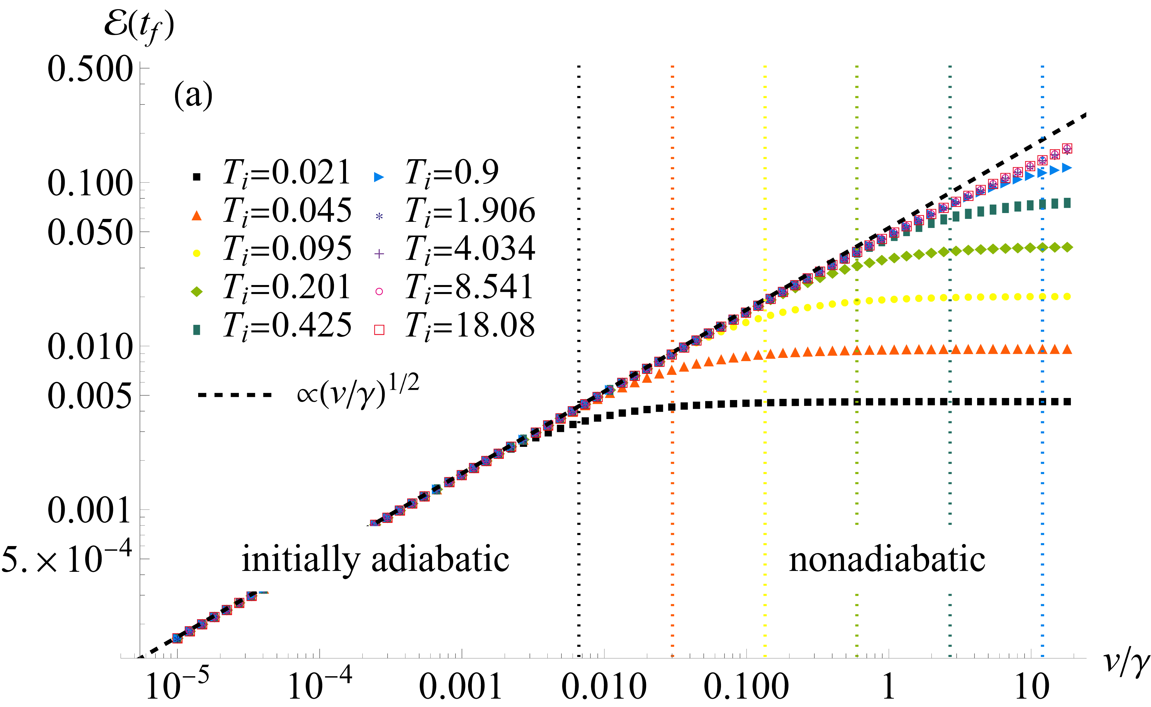
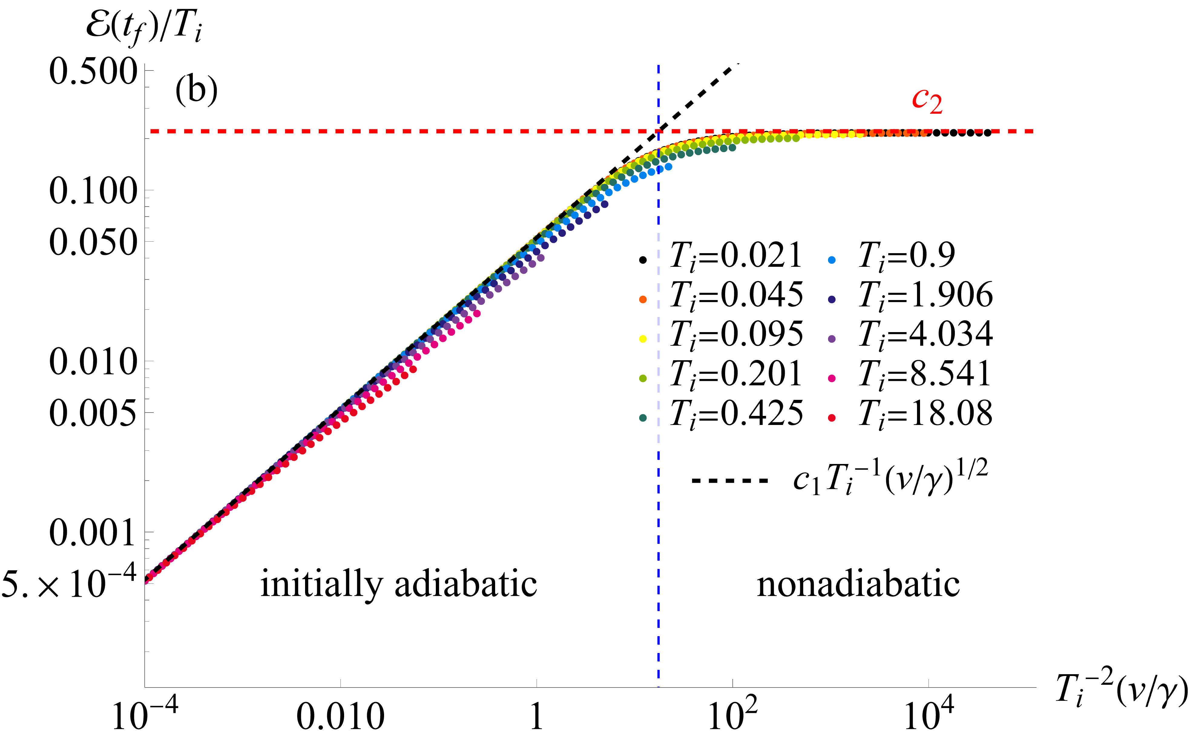
Figure S1: (a) The excitation density $\mathcal{E}$ at the end of the ramping protocol as a function of $v/\gamma$, shown for various initial temperatures $T_{i}$. Parameter values are $L=4\times 10^{4}$, $J=\Delta=1$, $\mu=-1$. Dotted vertical lines mark the crossover values between adiabatic and nonadiabatic regimes. The dashed black line shows the line $\mathcal{E}\propto\sqrt{v/\gamma}$ on which the data come to lie asymptotically for $T_{i}\to\infty$, in which case the dynamics is initially adiabatic for arbitrarily large ramp rates. (b) As in (a), but showing the rescaled excitation density $\mathcal{E}T_{i}^{-1}$ vs. the rescaled ramp rate $(v/\gamma)T_{i}^{-2}$, which results in approximate data collapse onto a single curve. For larger values of $T_{i}$, the quality of the data collapse diminishes (not shown).

II Derivation of Eqs. (6)–(7b) of the main text

The starting point of this derivation is the rate equation (3) of the main text with a relaxation rate as in Eq. (4). We assume that, as it should, the cutoff frequency of the bath spectral density is chosen sufficiently large such that $\mathcal{J}(\lambda_{k})=\pi\delta\lambda_{k}^{s}$ holds for the physical situation under investigation. Changing to the new variable $x=T(t)/\lambda_{k}=(T_{i}-vt)/\lambda_{k}$ in the rate equation (4) we obtain

$$\frac{d\mathcal{P}_{k}}{dx}=\frac{2\pi\delta\gamma\lambda_{k}^{s+1}}{v}\coth[1/(2x)]\left[\mathcal{P}_{k}-\mathcal{P}_{k}^{\text{th}}(1/x)\right],$$ (S1)

which is a linear, first-order differential equation with nonconstant coefficients. According to Sec. 1.1.4 of Ref. [1], the differential equation

$$\frac{dy(x)}{dx}=f_{1}(x)y(x)+f_{0}(x)$$ (S2)

with arbitrary functions $f_{0}$ and $f_{1}$ has the solution

$$y(x)=Ce^{F(x)}+e^{F(x)}\int dx\,e^{-F(x)}f_{0}(x)\qquad\text{with}\qquad F(x)=\int{dxf_{1}(x)},$$ (S3)

where the constant $C$ is determined by the initial condition. Identifying $y$ with $\mathcal{P}_{k}$, $f_{1}(x)$ with $2\pi\delta\gamma\lambda_{k}^{s+1}v^{-1}\coth[1/(2x)]$, and $f_{0}(x)$ with $-f_{1}(x)\mathcal{P}_{k}^{\text{th}}(1/x)$, and furthermore fixing the integration constant and domain such that $\mathcal{P}_{k}(T_{i}/\lambda_{k})=\mathcal{P}^{\text{th}}(\lambda_{k}/T_{i})$, one obtains the excitation probability of the $k$th mode,

$$\mathcal{P}_{k}(x)=Ce^{F(x)}-\frac{2\pi\delta\gamma\lambda_{k}^{s+1}}{v}e^{F(x)}\int_{T_{i}/\lambda_{k}}^{x}dx^{\prime}e^{-F(x^{\prime})}\coth[1/(2x^{\prime})]\mathcal{P}^{\text{th}}(1/x^{\prime}),$$ (S4)

with

$$C=\mathcal{P}^{\text{th}}(\lambda_{k}/T_{i})\qquad\text{and}\qquad F(x)=\frac{2\pi\delta\gamma\lambda_{k}^{s+1}}{v}\int_{T_{i}/\lambda_{k}}^{x}dx^{\prime\prime}\coth[1/(2x^{\prime\prime})].$$ (S5)

For later analyses it is useful to make explicit the dependence of $\mathcal{P}_{k}(T/\lambda_{k})$ on the various parameters and on the initial temperature. To this end, we identify $\mathcal{P}_{k}(T/\lambda_{k})$ with the trivariate function

$$\mathcal{P}\left(\frac{T}{\lambda_{k}},\frac{T_{i}}{\lambda_{k}},\frac{\gamma\lambda_{k}^{s+1}}{v}\right)\equiv\mathcal{P}_{k}(T/\lambda_{k}),$$ (S6)

for which the expression following from Eqs. (S4) and (S5) appears in (7a) and (7b) of the main text. The excitation density (5) is defined as a sum over the mode occupations $\mathcal{P}_{k}$, which, in the limit of large system size, can be replaced by the integral

$$\mathcal{E}(T,T_{i},\gamma/v)=\frac{1}{\pi}\int_{0}^{\pi}{dk\,\mathcal{P}\left(\frac{T}{\lambda_{k}},\frac{T_{i}}{\lambda_{k}},\frac{\gamma\lambda_{k}^{s+1}}{v}\right)},$$ (S7)

where we have exploited the $k\leftrightarrow-k$ mode symmetry to halve the integration domain. At the quantum critical point the energies of the low-lying modes are given, to leading order in $k$, by $\lambda_{k}=c|k|^{z}$ [2] with $c$ a constant and $z$ the equilibrium dynamical critical exponent. Within this low-energy approximation, we extend the upper bound of the integral in Eq. (S7) to infinity and perform the change of variables $k\rightarrow(\lambda/c)^{1/z}$, which yields Eq. (6) of the main text.

III Asymptotic behavior of the excitation density in Eqs. (6)–(7b) of the main text

To establish the asymptotic behavior of $\mathcal{E}(0,T_{i},\gamma/v)$ in the limit of large $T_{i}$, we prove below that

$$\lim_{y\to\infty}\mathcal{E}(0,y,1)=c_{1},$$ (S8)

with $c_{1}$ a finite, nonzero constant. Then it follows from Eq. (9) of the main text that

$$\lim_{T_{i}\to\infty}\mathcal{E}(0,T_{i},\gamma/v)=(\gamma/v)^{-1/[z(s+1)]}c_{1},$$ (S9)

which accounts for the plateaux in Figs. 2(b) and 2(c) of the main text. To establish the limit in Eq. (S8) we use Lebesgue’s dominated convergence theorem. First we apply integration by parts in Eq. (7a) to write

$$\mathcal{P}\left(0,y/\lambda,\lambda^{s+1}\right)=\int_{0}^{y/\lambda}dx^{\prime}\,\left[\frac{d}{dx^{\prime}}\mathcal{P}^{\text{th}}(1/x^{\prime})\right]\exp\left[-\lambda^{s+1}f(x^{\prime},0)\right].$$ (S10)

From Eq. (7b) it follows that $f(x^{\prime},0)$ is positive and quadratically increasing for large $x^{\prime}$, hence the factor $\exp[-\lambda^{s+1}f(x^{\prime},0)]$ is exponentially damped in $x^{\prime}$. The term in square brackets in Eq. (S10), which is a derivative of the Fermi-Dirac distribution, is positive and finite on the domain of integration and tends to zero for large $x^{\prime}$. As a result, the integral of the product of the two terms converges and is finite also in the limit of the domain of integration extending to $+\infty$. Since the integrand is positive it holds that $0<\mathcal{P}\left(0,y/\lambda,\lambda^{s+1}\right)<\mathcal{P}(0,\infty,\lambda^{s+1})$. Next we seek a bound on $\mathcal{P}(0,\infty,\lambda^{s+1})$. Returning to the integrand in Eq. (S10), we note that since $f(x^{\prime},0)\geqslant 2\pi\delta x^{\prime}$ it holds that $\exp[-\lambda^{s+1}f(x^{\prime},0)]\leqslant\exp(-2\pi\delta\lambda^{s+1}x^{\prime})$, and also that the derivative in the square brackets is bounded from above by $\exp(-1/x^{\prime})/x^{\prime 2}$. Together, this allows us to bound the integrand of $\mathcal{E}(0,y,1)$ in Eq. (S8), see also Eq. (6), as

$$0\leqslant\lambda^{1/z-1}\mathcal{P}\left(0,y/\lambda,\lambda^{s+1}\right)\leqslant\lambda^{1/z-1}\mathcal{P}\left(0,\infty,\lambda^{s+1}\right)\leqslant\lambda^{1/z-1}\int_{0}^{\infty}dx^{\prime}\,\frac{1}{x^{\prime 2}}e^{-1/x^{\prime}}\exp(-2\pi\delta\lambda^{s+1}x^{\prime})\equiv U(\lambda).$$ (S11)

Using Eq. 10.32.10 from Ref. [3] we find that $U(\lambda)=2\lambda^{1/z-1}\sqrt{b}K_{1}(2\sqrt{b})$, with $b=2\pi\delta\lambda^{s+1}$ and $K_{1}$ a modified Bessel function of the second kind. Note that $z\leqslant 1$ in all the cases we consider. The asymptotic behavior of $K_{1}$ in Eq. 10.40.2 of Ref. [3] now implies that $U$ behaves as $U(\lambda)\sim\lambda^{1/z-1}\sqrt{\pi}b^{1/4}e^{-2\sqrt{b}}$ in the limit of large $\lambda$. It follows that the integral $\int_{0}^{\infty}d\lambda\,U(\lambda)$ converges, which then implies the existence of the limit in Eq. (S8).

The asymptotic behavior of $\mathcal{E}(0,T_{i},\gamma/v)$ in the limit of small $T_{i}$ can be established by proving that

$$\lim_{y\searrow 0}\mathcal{E}(0,1,y)=c_{2},$$ (S12)

with $c_{2}=\ln 2/(\pi\lvert\Delta\rvert)$, which follows when inserting $\mathcal{P}(0,1/\lambda,0)=[\exp(\lambda)+1]^{-1}$ into Eq. (6) of the main text and setting $z=1$. Then it follows from Eq. (10) of the main text that

$$\lim_{T_{i}\searrow 0}\mathcal{E}(0,T_{i},\gamma/v)=T_{i}^{1/z}c_{2},$$ (S13)

which, when inserting the dynamical critical exponent $z=1$ of the Kitaev chain, accounts for the linear increases on the left-hand sides of Figs. 2(b) and 2(c) of the main text.

By similar techniques one can analyze the asymptotic behavior of $\mathcal{E}$ as a function of $v$, and the constant, respectively linear, regimes in Fig. S1 are recovered and characterized.

.

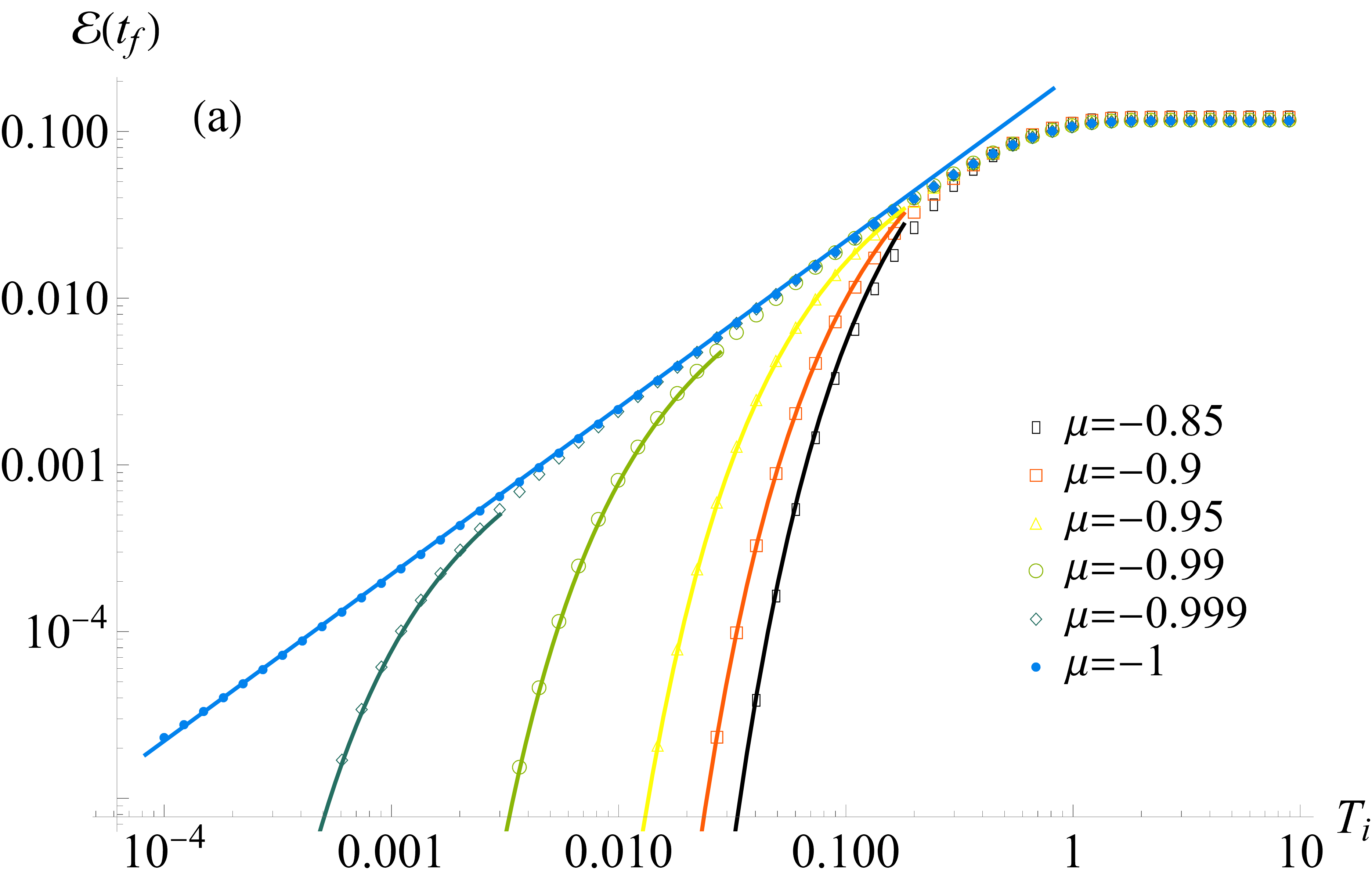
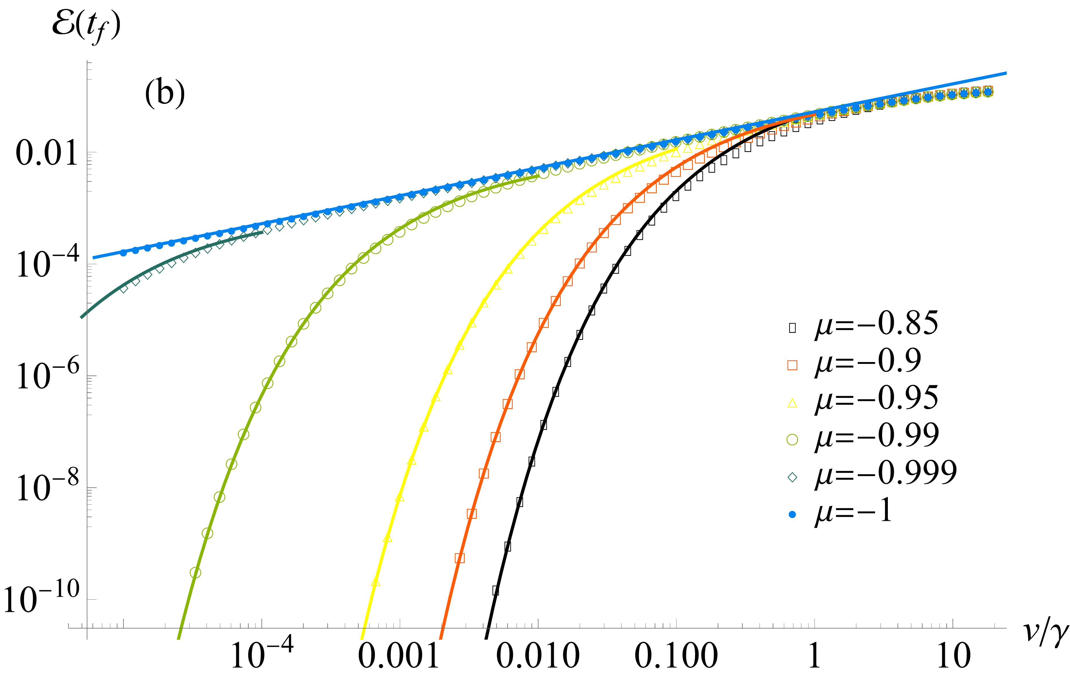
Figure S2: (a) The final excitation density $\mathcal{E}(t_{f})$ as a function of the initial temperature $T_{i}$, shown for protocols at various fixed noncritical values of the chemical potential $\mu$. Parameter values are $L=4\times 10^{4}$, $J=\Delta=1$, $\delta=1$, and $v/\gamma=8.1$. The solid blue line corresponds to the scaling result $\mathcal{E}\propto T_{i}$ for the ramp at $\mu=\mu_{c}=-1$, as in Fig. 2 of the main text. The asymptotic result in Eq. (S14) is shown for each value of $\mu\neq-1$ as a solid line in the corresponding color. (b) As in (a), but now showing $\mathcal{E}(t_{f})$ as a function of $v/\gamma$ for $T_{i}=0.9$. The solid blue line shows the scaling behavior $\mathcal{E}\propto\sqrt{v/\gamma}$ for cooling at $\mu=\mu_{c}=-1$, as in Fig. S1. The asymptotic results of Eq. (S15) for the cooling at $\mu\neq\mu_{c}$ are shown as solid lines in the corresponding colors.

IV Cooling protocols at fixed noncritical values of $\mu$

In the main text we considered cooling protocols at $\mu=\mu_{c}$ in order to probe aspects of the quantum critical behavior in the cleanest possible way. For cooling protocols at fixed noncritical values $\mu\neq\mu_{c}$, the asymptotic low-$T_{i}$ behavior of the excitation density is found to be

$$\mathcal{E}=\frac{1}{2}\sqrt{\frac{T_{i}}{\pi\lambda_{1}}}\exp\left(-\frac{\lambda_{0}}{T_{i}}\right),$$ (S14)

where $\lambda_{k}=\lambda_{0}+\lambda_{1}k^{2}$ is the low-energy approximation of the mode energies away from the critical point. In particular, we have $\lambda_{0}=2|\mu+J|$ and $\lambda_{1}=(\Delta^{2}-4J(\mu+J))/(4|\mu+J|)$ for the short-range Kitaev chain, and we consider parameter choices for which $\lambda_{1}>0$. Similarly, the small $v/\gamma$ behavior of the excitation density is given by

$$\mathcal{E}=\frac{1}{\sqrt{8}}\sqrt{\frac{\lambda_{0}}{\lambda_{1}}}\exp\left(-\sqrt{8\pi}\lambda_{0}\sqrt{\frac{\gamma}{v}}\right).$$ (S15)

The derivations of these asymptotic expressions, which are based on the rate equation solution in Eqs. (6)–(7b) of the main text, will be given elsewhere. In support of these results, Fig. S2 shows a comparison of the two asymptotic expressions for $\mathcal{E}$ with numeric data, where we plot the equivalents of Fig. 2(b) of the main text and Fig. S1(a), now for cooling protocols at fixed $\mu\neq\mu_{c}$. As Fig. S2 corroborates, the exponential factors in expressions (S14) and (S15) rule out any simple power-law scaling of $\mathcal{E}$ with either $T_{i}$ or $v/\gamma$ away from the critical point.

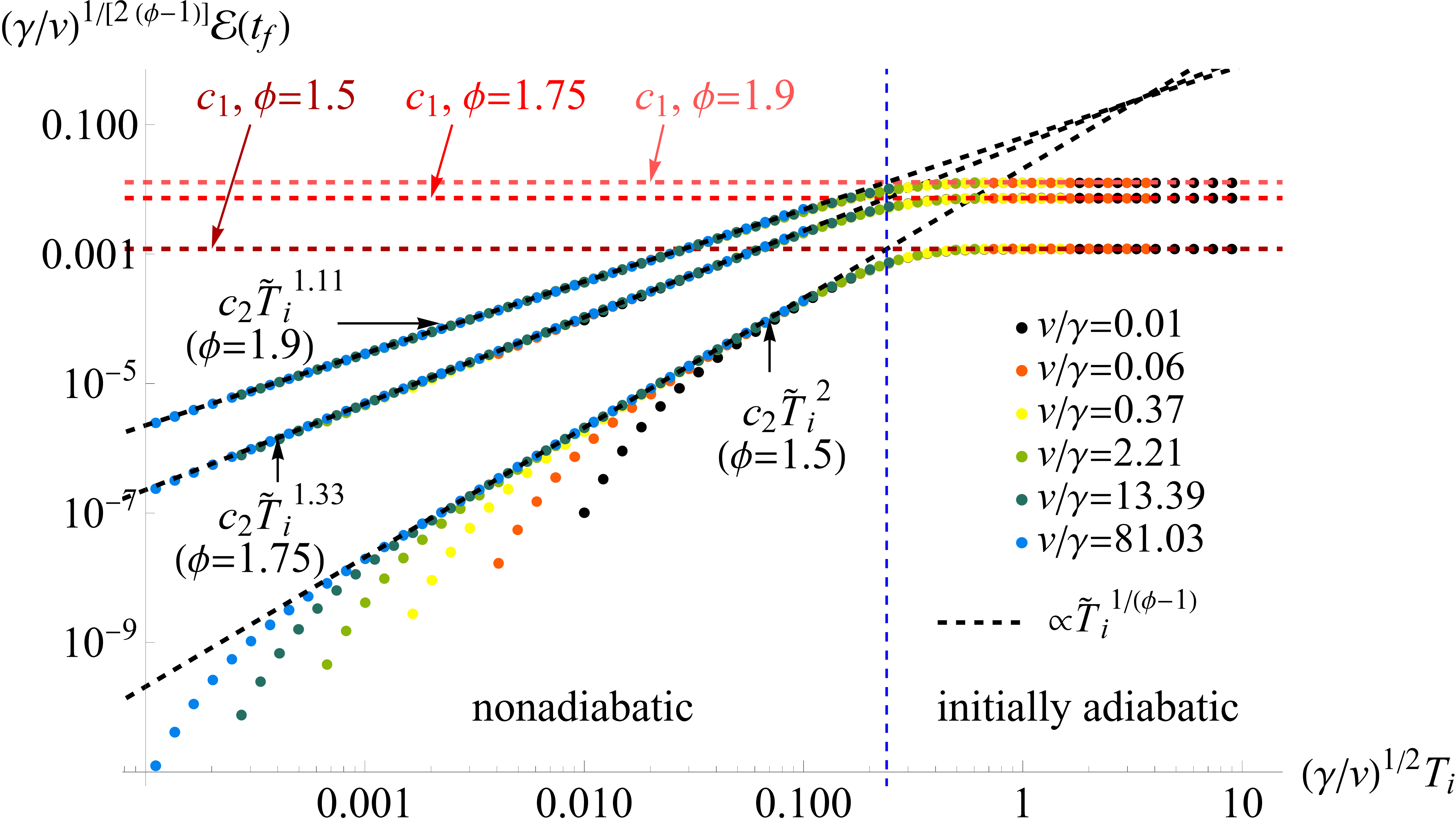
Figure S3: Rescaled excitation density $(\gamma/v)^{1/(2z)}\mathcal{E}$ at the end of a temperature ramp (3) as a function of the rescaled initial temperature $\widetilde{T}_{i}=\sqrt{\gamma/v}T_{i}$ for the Kitaev chain with long-range hopping (S16). Data is shown for the long-range hopping exponents $\phi=1.5$, $\phi=1.75$ and $\phi=1.9$, and for various ramp rates in each case, as indicated in the legend. For each data set, the corresponding asymptotic behaviors in the small-$\widetilde{T}_{i}$, respectively large-$\widetilde{T}_{i}$, regimes are shown as red and black dashed lines. Parameter values used are $L=4\times 10^{6}$, $J=\Delta=1$, $\delta=1$, and $\mu=\mu_{c}=-\zeta(\phi)$ [4, 5] given in terms of the Riemann zeta function $\zeta$.

V Nonequilibrium scaling of the long-range Kitaev chain

The interaction range of an interacting many-body system, or the hopping and/or pairing range of a quasifree many-body quantum system, can strongly affect the system’s properties. In particular, the critical behavior of long-range models, including the numerical values of critical exponents, usually differs from their short-range counterparts [6, 7, 8]. Hence, we also expect the scaling laws (8)–(10) for the cooling ramps to be influenced by the range.

We consider a Kitaev chain of length $L$ with long-range hopping and pairing [4],

$$H=J\sum_{j=1}^{L}{\sum_{l=1}^{\left\lfloor L/2\right\rfloor}{d_{l}^{-\phi}\left(c_{j}^{\dagger}c_{j+l}^{\vphantom{\dagger}}+c_{j+l}^{\dagger}c_{j}^{\vphantom{\dagger}}\right)}}+\frac{\Delta}{2}\sum_{j=1}^{L}{\sum_{l=1}^{\left\lfloor L/2\right\rfloor}{d_{l}^{-\alpha}\left(c_{j}^{\vphantom{\dagger}}c_{j+l}^{\vphantom{\dagger}}+c_{j+l}^{\dagger}c_{j}^{\dagger}\right)}}+2\mu\sum_{j=1}^{L}{c_{j}^{\dagger}c_{j}^{\vphantom{\dagger}}},$$ (S16)

with periodic boundary conditions. Different from the nearest-neighbor Hamiltonian (1) of the main text, hopping and pairing takes place between all pairs of sites. The corresponding hopping and pairing strengths decay like power laws proportional to $d_{l}^{-\phi}$ and $d_{l}^{-\alpha}$, respectively, where

$$d_{l}=\begin{cases}l&\text{for $l<L/2$},\\ 2^{1/\phi}l&\text{for $l=L/2$,}\end{cases}$$ (S17)

is a distance along the chain that takes into account the periodic boundary conditions. The factor of $2^{1/\phi}$ above will only survive in the hopping terms, where it prevents an overcounting of terms with a hopping range of $l=L/2$. In the limit of the long-range exponents $\phi$ and $\alpha$ going to infinity, the Kitaev chain with nearest-neighbor hopping and pairing (1) is recovered.

Just like the nearest-neighbor version, the Kitaev chain with long-range hopping and pairing (S16) is diagonalizable by means of a Bogoliubov transformation; see Ref. [4] and the companion paper [5] for details. The presence of long-range terms leads to a richer phase diagram [9, 10], and also to modified quantum critical exponents once $\phi$ or $\alpha$ become sufficiently small [4]. It is this latter property which we are going to probe by means of temperature ramps toward quantum criticality. The solvability of the long-range Kitaev chain, as in the nearest-neighbor case, also extends to the corresponding Lindblad equation describing the system coupled to bosonic baths, which can be diagonalized in Liouville space by the method of Third Quantization [11]; see Ref. [5] for details.

In Fig. S3 we plot data equivalent to that of Fig. 2 of the main text, but for the Kitaev chain with long-range hopping for various values of the long-range exponent $\phi$. For this model the dynamical critical exponent is

$$z=\begin{cases}\phi-1&\text{for $1\leqslant\phi\leqslant 2$},\\ 1&\text{for $2\leqslant\phi$}.\end{cases}$$ (S18)

According to the scaling law (9) of the main text, data collapse is obtained by plotting the rescaled excitation density $(\gamma/v)^{1/(2z)}\mathcal{E}$ at the end of a temperature ramp as a function of the rescaled initial temperature $\widetilde{T}_{i}=\sqrt{\gamma/v}T_{i}$. Hence, according to (S18), for $\phi\in[1,2]$ the rescaling has to be performed with a $\phi$-dependent exponent, which is nicely confirmed by Fig. S3. According to the scaling laws of the main text, also the slope of the asymptotic behavior on the left-hand side of the plot becomes $\phi$-dependent in that case, $(\gamma/v)^{1/(2z)}\mathcal{E}\propto\widetilde{T}_{i}^{1/(\phi-1)}$, which again is confirmed by the data of Fig. S3. The deviation from the asymptotic behavior at low initial temperatures is due to finite-size effects. Similar results are obtained for the case of long-range pairing (not shown). Note that the nonequilibrium scaling of temperature ramps in the long-range Kitaev chain is governed by the equilibrium critical exponents of the underlying quantum phase transitions, even in the regime where deviations from such behavior were found for parameter ramps [12].

References

• Polyanin and Zaitsev [2002] A. D. Polyanin and V. F. Zaitsev, Handbook of Exact Solutions for Ordinary Differential Equations, 2nd ed. (Chapman and Hall/CRC, New York, 2002).
• Dutta et al. [2015] A. Dutta, G. Aeppli, B. K. Chakrabarti, U. Divakaran, T. F. Rosenbaum, and D. Sen, Quantum Phase Transitions in Transverse Field Spin Models: From Statistical Physics to Quantum Information (Cambridge University Press, Cambridge, 2015).
• Olver et al. [2010] F. W. J. Olver, D. W. Lozier, R. F. Boisvert, and C. W. Clark, eds., NIST Handbook of Mathematical Functions (Cambridge University Press, Cambridge, 2010).
• Vodola et al. [2016] D. Vodola, L. Lepori, E. Ercolessi, and G. Pupillo, Long-range Ising and Kitaev models: Phases, correlations and edge modes, New J. Phys. 18, 015001 (2016).
• [5] E. King, M. Kastner, and J. N. Kriel, Long-range Kitaev chain in a thermal bath: Analytic techniques for time-dependent systems and environments, arXiv:2204.07595 .
• Fisher et al. [1972] M. E. Fisher, S.-K. Ma, and B. G. Nickel, Critical exponents for long-range interactions, Phys. Rev. Lett. 29, 917 (1972).
• Dutta and Bhattacharjee [2001] A. Dutta and J. K. Bhattacharjee, Phase transitions in the quantum Ising and rotor models with a long-range interaction, Phys. Rev. B 64, 184106 (2001).
• Defenu et al. [2020] N. Defenu, A. Codello, S. Ruffo, and A. Trombettoni, Criticality of spin systems with weak long-range interactions, J. Phys. A 53, 143001 (2020).
• Viyuela et al. [2016] O. Viyuela, D. Vodola, G. Pupillo, and M. A. Martin-Delgado, Topological massive Dirac edge modes and long-range superconducting Hamiltonians, Phys. Rev. B 94, 125121 (2016).
• Bhattacharya and Dutta [2018] U. Bhattacharya and A. Dutta, Topological footprints of the Kitaev chain with long-range superconducting pairings at a finite temperature, Phys. Rev. B 97, 214505 (2018).
• Prosen [2008] T. Prosen, Third quantization: A general method to solve master equations for quadratic open Fermi systems, New J. Phys. 10, 043026 (2008).
• Defenu et al. [2019] N. Defenu, G. Morigi, L. Dell’Anna, and T. Enss, Universal dynamical scaling of long-range topological superconductors, Phys. Rev. B 100, 184306 (2019).