The long-active afterglow of GRB 210204A: Detection of the most delayed flares in a Gamma-Ray Burst

Abstract

We present results from extensive broadband follow-up of GRB 210204A over the period of thirty days. We detect optical flares in the afterglow at $7.6\times 10^{5}$ s and $1.1\times 10^{6}$ s after the burst: the most delayed flaring ever detected in a GRB afterglow. At the source redshift of 0.876, the rest-frame delay is $5.8\times 10^{5}$ s (6.71 d). We investigate possible causes for this flaring and conclude that the most likely cause is a refreshed shock in the jet. The prompt emission of the GRB is within the range of typical long bursts: it shows three disjoint emission episodes, which all follow the typical GRB correlations. This suggests that GRB 210204A might not have any special properties that caused late-time flaring, and the lack of such detections for other afterglows might be resulting from the paucity of late-time observations. Systematic late-time follow-up of a larger sample of GRBs can shed more light on such afterglow behaviour. Further analysis of the GRB 210204A shows that the late time bump in the light curve is highly unlikely due to underlying SNe at redshift (z) = 0.876 and is more likely due to the late time flaring activity. The cause of this variability is not clearly quantifiable due to the lack of multi-band data at late time constraints by bad weather conditions. The flare of GRB 210204A is the latest flare detected to date.

1 Introduction

Long Gamma-Ray Bursts (GRBs) originate from the core collapse of massive stars (Kouveliotou et al., 1993; Kumar & Zhang, 2015). The GRB emission consists of two distinct phases: the prompt emission typically observed in soft $\gamma$-rays and hard X-rays, and the afterglow, which has been detected across a wide range of wavelengths from radio to TeV band (Piran, 2004; MAGIC Collaboration et al., 2019).

GRB prompt emission is created by energy dissipation as the relativistic jet accelerates particles via either internal shocks or magnetic reconnection (Pe’er, 2015). These particles typically emit a non-thermal spectrum that is often dominated by synchrotron radiation (Burgess et al., 2020; Zhang, 2020). However, the detailed radiation physics of GRBs is not fully understood (Kumar & Zhang, 2015). In practice, the prompt GRB spectrum is usually modelled phenomenologically as a “Band” spectrum (Band et al., 1993). In addition, some spectra show additional features such as thermal components or multi-coloured blackbody peaks (Pe’Er & Ryde, 2017), inverse Compton scattered components (Derishev et al., 2001), low energy spectral breaks (Oganesyan et al., 2018), deviation from synchrotron spectra (Daigne et al., 2011), etc. The physical/spectral parameters of prompt emission — like the Lorentz Factor $\Gamma$, the peak energy $E_{\rm p}$, the isotropic equivalent energy $E_{\gamma,\mathrm{iso}}$, or the isotropic luminosity $L_{\gamma,\mathrm{iso}}$ — show some correlations like the Amati correlation (Amati, 2006), which have been explored for understanding GRB properties as well as applying them for cosmology.

The interaction of the jet with the ambient medium gives rise to synchrotron emission, commonly known as the afterglow (Mészáros & Rees, 1997; Sari et al., 1998; Piran, 2005). The afterglow is broadband and lasts much longer than the GRB: being visible for hours to days in X-ray bands, days to weeks in optical, and weeks to months at radio wavelengths. From the first afterglow detection by BeppoSAX (GRB 970228; Costa et al., 1997), the understanding of afterglows has increased tremendously over the decades — with a huge boost from the Neil Gehrels Swift Observatory with its rapid response abilities (Gehrels et al., 2004). The afterglow emission is phenomenologically simple to model, and the flux $F$ is often fit by a simple power-law in both time and frequency, $F\propto t^{-\alpha}\nu^{-\beta}$. The temporal decay index $\alpha$ and spectral decay index $\beta$ typically follow the $\alpha-\beta$ closure relation predicted by the forward shock model (Zhang, 2021; Piran, 2005). Some GRB afterglows show features that provide insights into the physics of the source: for instance, jet breaks (Rhoads, 1999; Sari et al., 1999), supernovae in long GRBs (Galama et al., 1998; Galama et al., 1999), and flaring activity generated by various mechanisms (Burrows et al., 2005b; Falcone et al., 2007).

GRB 210204A, first reported by Fermi Gamma-Ray Burst Monitor (GBM), is a long GRB with multiple pulses in the prompt emission (Meegan et al. 2009). The optical afterglow was detected by the Zwicky Transient Facility  (ZTF; Bellm, 2014) and followed by multiple observatories in many wavebands. Here, we report our findings based on extensive follow-up of the source with multiple telescopes. The paper is organised as follows. In §2, we describe our observations and data reduction. We also list out public data from various sources that we have used in this work. §3 discusses the temporal and spectral characteristics of the prompt emission. In §4 we undertake broadband modelling of the afterglow, showing clear evidence of late-time brightening. We conclude by discussing various causes for this in §5 and identifying the most plausible one.

2 Observations and data analysis

In this section, we present the prompt and afterglow observations carried out by various space and ground-based telescopes.

2.1 Prompt Emission

GRB 210204A was discovered by the Fermi (GBM, Meegan et al. 2009) at UT 2021-02-04 06:29:25 (hereafter, T₀). The source was first localised to RA = 109.1°, Dec = 9.7° (J2000) with a statistical uncertainty of 4.0°  (Fermi GBM Team, 2021). The burst was also detected by Gravitational-wave high-energy Electromagnetic Counterpart All-sky Monitor (GECAM-B, Li et al. 2021), Konus-Wind (Frederiks et al., 2021), and AstroSat (Waratkar et al., 2021). The source localisation was refined by  BALROG  (Kunzweiler et al., 2021), and further by the Inter-Planetary Network (IPN) by using data from Fermi, Integral,  Swift, Konus-Wind, and Mars-Odyssey-HEND (Hurley et al., 2021).

In this section, we focus on the analysis of data from Fermi and AstroSat (Figure 1).

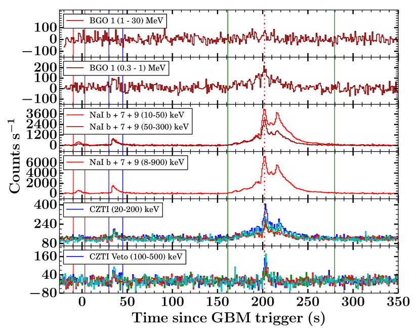
Figure 1: Top four panels: Energy-resolved Fermi-GBM prompt emission light curves (back-ground subtracted) of GRB 210204A. The vertical red, blue and green lines indicate the duration of the first, second, and third episodes, respectively. The vertical dashed-dotted line indicates the peak used to calculate the isotropic luminosity of the burst. Bottom two panels: AstroSat-CZTI light curves in 20-200 keV and 100-500 keV energy range for GRB 210204A. The four colours (blue, green, red, and cyan) correspond to data from four quadrants (A, B, C, and D) of the instrument. The GRB is detected more prominently in quadrants A and D due to the location of the GRB on the sky.

2.1.1 Fermi-GBM

We retrieved the Fermi-GBM data (the time-tagged event (TTE) mode) of GRB 210204A from the Fermi Science Support Center archives. We performed the temporal and spectral analysis of GBM data using three sodium iodide (NaI) detectors (NaI b, NaI 7, and NaI 9) and one bismuth germanate (BGO) detector (BGO 1). These detectors have following GRB observing angles NaI b: $\rm 25^{\circ}$ degree, NaI 7: $\rm 35^{\circ}$ degree, NaI 9: $\rm 47^{\circ}$, and BGO1: $\rm 25^{\circ}$, respectively. For the temporal analysis of Fermi-GBM data, we utilized RMFIT version 4.3.2 software and generated the prompt emission background subtracted light curve of GRB 210204A in different energy ranges. Furthermore, we performed the spectral analysis of Fermi-GBM data using the Multi-Mission Maximum Likelihood framework (Vianello et al., 2015, 3ML). We performed time-integrated as well as time-resolved spectral analysis of GBM data to constrain the possible emission mechanisms of GRB 210204A. We started the spectral modelling using traditional GRB model called Band or GRB function (Band et al., 1993). In addition to Band function, we explore various other possible models such as simple power-law model, a power-law model with a high energy spectral cutoff (cutoffpl), Black Body function to search for photospheric signature in the spectrum, a power-law function with two sharp spectral breaks (bkn2pow), or combination of these models. We utilised the deviance information criterion (DIC; Spiegelhalter et al., 2002) to find the best fit model. A more detailed methodology for GBM data analysis is discussed in Gupta et al. (2021b, 2022).

2.1.2 AstroSat CZTI

AstroSat Cadmium Zinc Telluride Imager (CZTI; Bhalerao et al., 2017) detected the second and third pulse of GRB 210204A, with a total of 18141 photons: 94% of which came from the brighter third pulse (Waratkar et al., 2021; Sharma et al., 2020). These two pulses were also clearly seen in the veto detectors. In detector coordinates, the GRB was incident from $\theta=75.43\deg$ and $\phi=172.80\deg$: just 15° from the detector plane. CZTI can be used to measure the polarisation of GRBs by analysing two-pixel Compton events (Vadawale et al., 2015; Chattopadhyay et al., 2014). However, such measurements are robustly possible only for GRBs with $\theta<60\deg$ (Chattopadhyay et al., 2019) — ruling out the possibility of polarimetric studies of GRB 210204A.

2.2 Multiwavelength Afterglow

The large 4° positional uncertainty in the Fermi localisation precluded prompt follow-up observations by most telescopes. However, Kool et al. (2021) used the wide-field ZTF and reported the discovery of a fast optical transient ZTF21aagwbjr/AT2021buv, a candidate afterglow for GRB 210204A $\sim 38$ mins after the trigger. Subsequent follow-up observations by multiple telescopes verified the fading nature of this source and confirmed that it was indeed the afterglow of GRB 210204A.

2.2.1 X-ray afterglow

Equipped with the precise afterglow position, the Neil Gehrels Swift Observatory started Target-of-Opportunity observations of the GRB 210204A field about $1.6\times 10^{5}$ s after the initial burst (Evans & Swift Team, 2021). The Swift X-ray telescope (XRT; Burrows et al., 2005a) detected an uncatalogued X-ray source at RA, Dec = $117.08071\deg,+11.40951\deg$ (J2000), consistent with the optical position. Multiple observations obtained till $3\times 10^{5}$ s after the burst confirmed the fading nature of this source.

We used the XRT online repositories by Evans et al. (2007, 2009) to retrieve the light curves and spectra, respectively. We undertook spectral analysis with the X-Ray Spectral Fitting Package (XSPEC; Arnaud, 1996) version 12.10.1. The 0.3-10 keV spectra were modelled as a simple absorbed power-law (using the XSPEC phabs model). For the time-averaged XRT spectrum (from T₀ +1.61 $\times$ $10^{5}$ to T₀ + 1.73 $\times$ $10^{5}$ s), we get $\Gamma=1.73^{+0.28}_{-0.26}$, and $N_{\mathrm{H}}=6.43^{+5.40}_{-4.19}\times 10^{21}~{}\mathrm{cm}^{2}$. In Table LABEL:tab:xrt, we give the temporal evolution of XRT unabsorbed fluxes and photon indices (determined from the hardness ratio) obtained from the Swift Burst Analyser web page, supported by the UK Swift Science Data Centre.

2.2.2 Optical afterglow

Kool et al. (2021) discovered the afterglow about 38 minutes after the initial burst. They also reported a non-detection of the same object in serendipitous observations of the field about 1.9 hours prior to their first detection (see Andreoni et al. (2021) and Ho et al. (2022) for discovery details). Follow-up observations obtained by various groups (see for instance Table LABEL:tab:public) revealed that the source was indeed the fading afterglow of GRB 210204A and measured the source redshift. We embarked on an extensive monitoring campaign using various telescopes in the time interval between $\sim 0.03$ and $\sim 20$ days, after the burst event.

We discuss our observations from four Indian facilities in this section and present a summary of data reported by other groups.

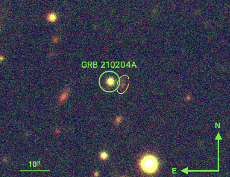
(a) DOT image of GRB

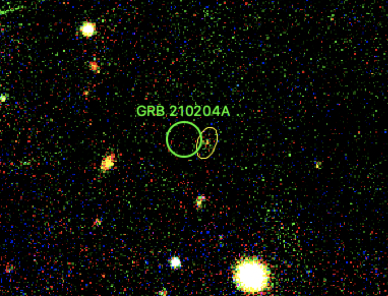
(b) Pan-STARRS DR1 image

Figure 2: GRB 210204A detection by the 4K $\times$ 4K CCD IMAGER mounted at the axial port of Devasthal Optical Telescope (DOT). (a) An image of GRB 210204A afterglow detection in DOT image. The position of afterglow is indicated by the green circle. There is a galaxy present at $\sim 4.4~{}\arcsec$ from the location of GRB (shown with a yellow ellipse), but it is unlikely to be the host (§2.2.2). (b) Snapshot of Pan-STARRS image of the same field is shown where no source is present at the position of afterglow.

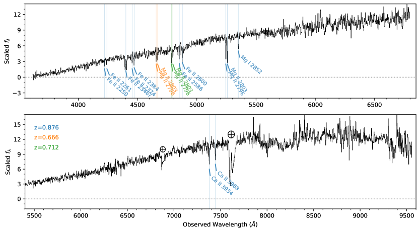
Figure 3: GMOS-S spectrum of ZTF21aagwbjr. The upper and bottom panel show the resulting spectrum in the blue and red gratings, respectively. We identify a number of strong, narrow absorption features of Fe ii, Mg ii, M i and Ca ii at a common redshift of $z=0.876$ (blue notations). We identify two additional intervening absorbers, based on Mg ii $\lambda\lambda$2796, 2803 at $z=0.666$ (orange notations) and $z=0.712$ (green notations).

We followed up GRB 210204A with the GROWTH-India Telescope (GIT), a 0.7 m telescope located at the Indian Astronomical Observatory, Ladakh. The telescope was equipped with a 2184$\times$1472 pixel Apogee KAF3200EB camera, giving a limited $11^{\prime}\times 7.5^{\prime}$ field of view. While poor observing conditions prevented immediate follow-up after the announcement of the ZTF discovery, our observations began on 2021 February 06, 2.36 days after the initial alert, and continued till March 1, 2021. Typical observations consisted of multiple 300 s exposures in the $\rm{r}^{\prime}$ filter, with each exposure having a limiting magnitude of $\sim 20.5$ mag. We used the 2.0 m  Himalayan Chandra Telescope (HCT) on three nights: 2021 February 07, 2021 February 12 and 2021 February 14, under proposal number HCT-2021-C1-P2. Data were obtained in Bessel V, R, and I filters (Table LABEL:table:phot-table-our). The 3.6 m Devasthal Optical Telescope (DOT), located at the Devasthal Observatory of Aryabhatta Research Institute of Observational Sciences (ARIES), Nainital, India (Sagar et al., 2019) was triggered under our ToO proposal number DOT-2021-C1-P62 (PI: Rahul Gupta) and DOT-2021C1-P19 (PI: Ankur Ghosh) for the follow up. We observed GRB 210204A on multiple epochs with the 4K $\times$ 4K CCD IMAGER (Pandey et al., 2018; Kumar et al., 2021). The first observations were obtained in BVRI filters (Gupta et al., 2021c), while data on subsequent nights were obtained in the SDSS r filter. Further, we also obtained data with the 1.3 m Devasthal Fast Optical Telescope (DFOT) located at Devasthal observatory of ARIES, Nainital, India (Sagar et al., 2011) under our ToO Proposal ID DFOT-2021A-P6 (PI: Rahul Gupta). We obtained data in B, V, R, and I filters on 2021-06-06 (T₀ + 2.4 d), and more data in R and I bands on 2021-02-13 UT.

Data obtained from all these facilities were reduced in similar manner using a python based reduction pipeline. Images were calibrated using bias and flat frames; pipeline made use of Astro-SCRAPPY (McCully & Tewes, 2019) python package to remove cosmic rays from the science images. Once the images were corrected for all artefacts, we solved the images for astrometry using astrometry.net solve-field engine (Lang et al., 2010) in offline mode. Sources in images were extracted in the form of a locally generated catalogue via SExtractor (Bertin & Arnouts, 1996). PSFEx astromatic software (Bertin, 2011) gave the PSF profile of the sources, which was used to get magnitudes of stars in the images. For images obtained in ugriz filters, these magnitudes were cross-matched with Panoramic Survey Telescope and Rapid Response System (Pan-STARRS) DR1 catalogue (Chambers et al., 2016) and Sloan Digital Sky Survey (SDSS) DR12 catalogue (Alam et al., 2015) using VizieR to get the zero-points of the images. While, for BVRI filter images, we used data from Sloan Digital Sky Survey (SDSS) (Alam et al., 2015) and converted the magnitudes to VRI bands using Lupton (2005) transformations to estimate the zero-points. For later epochs where the afterglow was fainter, multiple exposures were stacked together using SWarp (Bertin et al., 2002). Table LABEL:table:phot-table-our lists the magnitudes with 1-sigma uncertainties. In case the source was not detected, we report 5-sigma upper limits.

In addition to the observations taken by our group, we also use publicly available data reported in Gamma-ray Coordination Network (GCN) by various groups. This set includes data from the ZTF published in (Andreoni et al., 2021), 1.6-m AZT-33IK telescope, 70 cm AS-32 telescope (Molotov et al., 2009), Large Binocular Telescope Hill (2010), 2.6-m Shajn Telescope (Ioannisiani et al., 1976) and the AZT-20 at Assy-Turgen observatory. These data, along with the GCN references, are tabulated in Table LABEL:tab:public.

Figure 2 shows the detection of GRB afterglow with DOT (located by the green circle in the image). In DOT images, a galaxy is present $\sim 4.4~{}\arcsec$ away from the afterglow position. This transforms to a physical distance of $\sim 33$ kpc from GRB location, which is rather large for the galaxy to be the host of GRB 210204A. Further, the photometric redshift of this galaxy is $z_{\mathrm{phot}}=0.436$ makes it implausible to be the host of GRB 210204A.

Spectroscopy: We triggered a long-slit spectrum of GRB 210204A with GMOS-S under our ToO program GS-2021A-Q-124 (PI: A. Ho). The observation, conducted in the Nod-and-Shuffle mode with a 1″wide slit, started at 2021-02-06 01:19:09.2 UT, corresponding to 42.8 hours after the Fermi-GBM trigger. We obtained $2\times 450$ s spectroscopic exposures with the B600 grating and $2\times 450$ s exposures with the R400 grating, providing coverage over the range 3620–9600 Å. Flux calibration was not performed. The spectrum was reduced using the IRAF package for GMOS. We identified a series of strong absorption features at $z=0.876$ superposed on a relatively flat, featureless continuum (Figure 3).

We also detected intervening absorption systems of Mg ii $\lambda\lambda$2796, 2803 at $z=0.666$ and $z=0.712$. This interpretation is consistent with that of Izzo et al. (2021), who obtained spectra using ESO VLT UT3 equipped with X-shooter spectrograph $~{}\sim 1.79$ days after the trigger. Their spectra spanned the wavelength range from 3000-21000 $\AA$ in which they report a few absorption lines of Al II, Ca II, Fe II, Mg I, Mg II, Zn II, Ca H and K detected at a common redshift of z = 0.876. They also detect three intervening Mg II absorbers at redshifts of z = 0.71, 0.66, and 0.57.

2.2.3 Radio afterglow

The GRB 210204A event was triggered with the upgraded Giant Metrewave Radio Telescope (uGMRT) at 2021 Feb 20.56 UT in band 5 (1000–1450 MHz). The observations were two hours in duration, including overheads using a bandwidth of 400 MHz. We use the Common Astronomy Software Applications (CASA; McMullin et al., 2007) for data analysis. The data were analysed in three major steps, i.e. flagging, calibration and imaging using the procedure laid out in Maity & Chandra (2021). A source was clearly detected at the RA(J2000) = 07:48:19.34, Dec(J2000) = 11:24:33.91. This position is consistent with the position reported by ZTF for the GRB (Kool et al., 2021). Further follow-up observations were triggered on 2021 Mar 07.59 UT and 2021 Mar 09.56 UT in the uGMRT band 4 and band 5 respectively, 2 hours at each band including overheads. In both observation the source was detected with a resolution of $2.66\arcsec\times 1.74\arcsec$ and $6.87\arcsec\times 2.05\arcsec$. Table LABEL:tab:radio lists the detailed radio followup information.

3 Prompt emission

We analyse the Fermi data of the prompt emission to characterise GRB 210204A and compare it with the overall GRB population.

3.1 Spectral analysis of the complete GRB

The prompt emission light curve of GRB 210204A obtained using Fermi-GBM data shows three distinct episodes, separated by quiescent temporal gaps (see Figure 1). The first two episodes have relatively faint and simple fast rising and exponential decay profiles, but the third and brightest episode has rich sub-structure. The $T_{\rm 90}$ duration for the entire burst is 207.86 $\pm$ 0.06 s. The time-integrated (the entire duration of the burst) Fermi-GBM spectrum (from T₀-9.73 to T₀ +279.55 s) could be best explained using traditional Band plus Blackbody model with following spectral parameters: peak energy ($E_{\rm p}$) = $146\pm 14$ keV, low energy spectral index $\alpha_{\rm pt}=-1.30\pm 0.07$, high energy spectral index $\beta_{\rm pt}=-2.39^{+0.17}_{-0.18}$ and temperature kT_BB $=6.5\pm 0.6$ keV.

Table 1: Comparison between the characteristics of three episodes of GRB 210204A. The quiescent duration between the first two episodes is $\sim 26.2~{}$s, while that between the second and third episode is $\sim 116.2~{}$s. A blackbody component is needed only for the third episode (§3.2). All reported values are observer frame values. The total energy and luminosity were calculated using the source redshift $z=0.876$. $\rm T_{90}$: Duration in 50–300 keV band; HR: ratio of the counts in 50 - 300 ${\rm keV}$ to the counts in 10 - 50 ${\rm keV}$; $\rm E_{p}$, $\alpha$, $\beta$: Band spectral fit parameters; $\rm F$: Bolometric energy flux; $\rm E_{\gamma,iso}$: Isotropic energy; $\rm L_{p,iso}$: Isotropic peak luminosity

Characteristics	Episode 1	Episode 2	Episode 3
$T_{\rm 90}$ (s) in 50 - 300 keV	$12.04\pm 0.02$	$12.81\pm 0.04$	$82.66\pm 0.05$
HR	0.41	0.79	0.57
$E_{\rm p}$ (keV)	$36\pm 9$	$197\pm 30$	$146\pm 9$
$\alpha$	$-0.96\pm 0.36$	$-1.21\pm 0.07$	$-1.30\pm 0.04$
$\beta$	$-2.14\pm 0.14$	$-2.6\pm 0.3$	$-2.46\pm 0.14$
kTBB	$\cdots$	$\cdots$	$6.39\pm 0.40$
$\rm F$ ($\rm 10^{-7}erg~{}cm^{-2}~{}s^{-1}$)	$1.6_{-1.13}^{+3.65}$	$3.8_{-0.7}^{+0.9}$	$7.9\pm 1$
$\rm E_{\gamma,iso}$ ($\rm erg$)	$4.19\times 10^{51}$	$1.22\times 10^{52}$	$1.94\times 10^{53}$
$\rm L_{p,iso}$ ($\rm erg~{}s^{-1}$)	$1.80\times 10^{51}$	$4.44\times 10^{51}$	$1.70\times 10^{52}$

3.2 Episode-wise analysis

If we analyse the three pulses separately, we see that the $E_{\rm p}$ values for the second and third pulses are higher (Table 1). We find that the band function gives acceptable spectral fits to the first and second episodes. The third episode is better fit by a power-law with two breaks (bkn2pow) or by a Band spectrum with an added blackbody component. The thermal component has a temperature of $6.4\pm 0.4$ keV. We use the Band + blackbody model in the rest of this section. We note that due to the lower intensity of the first two episodes, the data quality is not high enough to rule out such spectral features in them.

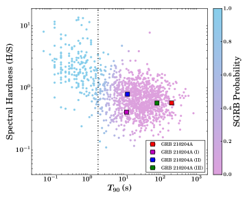
Figure 4: Prompt emission $T_{\rm 90}$-HR correlations: (a) Time-integrated (shown with a red square), and episode-wise (shown with magenta, blue, and green squares for the first, second, and third episodes, respective) $T_{\rm 90}$-HR correlation for GRB 210204A. We have also shown the data points for long and short GRBs taken from Goldstein et al. (2017). The right side y scale shows the probability of short GRBs. The vertical black dashed-dotted line indicates the boundary between two classes of GRBs.

The presence of a thermal component along with a non-thermal component indicates a hybrid jet composition, including a matter-dominated hot fireball and a colder magnetic-dominated Poynting flux component for GRB 210204A. The low energy spectral index values (Table 1) are within the range expected for synchrotron emission, $-3/2<\alpha<-2/3$.

We calculated the $T_{\rm 90}$ values and the (50 – 300 keV)/(10 – 50 keV) hardness ratios for the entire GRB and the three episodes within it. Following Narayana Bhat et al. (2016), we estimated the errors in these by simulating 10,000 light curves by adding Poisson noise with mean equal to observed values and repeating these measurements on each simulated light curve. Figure 4 shows these values compared to the population of long and short GRBs — we find that GRB 210204A, as well as the three individual emission episodes within it, are all consistent with the “long–soft” GRB population.

3.3 GRB global relationships

The time-integrated rest-frame peak energy ($E_{\rm p,i}$) of the prompt emission spectrum of GRBs is correlated to the isotropic equivalent energy ($E_{\gamma,\rm iso}$), and this correlation is defined as Amati correlation (Amati, 2006). Basak & Rao (2013) studied the episode-wise Amati correlation for a sample of Fermi-GBM detected GRBs with a measured redshift and confirmed that this correlation is more robust and valid for the episode-wise activity of GRBs. Recently, Chand et al. (2020) studied the Amati correlation for a sample of two-episodic GRBs and found that other than the first episode of GRB 190829A, each episode of two-episodic GRBs are consistent with the Amati correlation. In addition to GRB 190829A, a few other GRBs such as GRB 980425B, GRB 031203A, and GRB 171205 do not follow the Amati correlation.

Another variant of Amati correlation is Yonetoku correlation which is the correlation between time-integrated rest-frame peak energy ($E_{\rm p,i}$) and isotropic peak luminosity $L_{\rm\gamma,iso}$ (Yonetoku et al., 2004). These correlations have been utilised to classify individual episodes in GRBs with long quiescent phases. Figure 5 shows GRB 210204A on the Amati and Yonetoku correlations. We find that the time-integrated, as well as individual episodes values, are consistent with the Amati correlation of typical long GRBs. Similarly, the $L_{\rm\gamma,iso}$, and $E_{\rm p,i}$ values for individual episodes are consistent with the Yonetoku correlation.

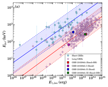
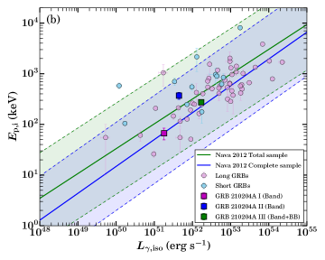
Figure 5: Prompt emission Amati and Yonetoku correlations: (a) Time-integrated (shown with a red square), and episode-wise (shown with magenta, blue, and green squares for the first, second and third episodes, respective) Amati correlation for GRB 210204A. Note that the $E_{\rm p}$ values have been converted to the rest frame using the GRB redshift $z=0.876$. We also show the data points for long and short GRBs taken from Minaev & Pozanenko (2020). The red and blue solid lines show the best-fit line for long and short bursts, and the shaded regions represent the 2-$\sigma$ uncertainty region for both the populations of GRBs. (b) The episode-wise (shown with magenta, blue, and green squares for the first, second and third episodes, respective) Yonetoku correlation for GRB 210204A. We also show the data points for long and short GRBs taken from Nava et al. (2012). The green and blue solid lines show the best-fit line, and the shaded regions represent the 3-$\sigma$ uncertainty region.

4 Afterglow

The GRB blast-wave interacts with the circumburst medium giving rise to synchrotron emission, which is one of the primary signatures of standard GRB fireball model (Granot & Sari, 2002). The electrons have a power-law energy distribution characterised by the index p, which results in the spectral energy distribution, which can be described as a series of multiple power-law segments. These segments join each other a particular frequencies known as break frequencies i.e. self absorption frequency ($\nu_{\mathrm{sa}}$), cooling frequency ($\nu_{\mathrm{c}}$), and synchrotron frequency ($\nu_{\mathrm{m}}$). In optical and X-rays emission, synchrotron self-absorption does not play an important role and hence can be neglected. Depending on the ordering of two break frequencies $\nu_{\mathrm{c}}$ and $\nu_{\mathrm{m}}$, multiple spectral regimes are possible, which in turn govern the overall shape of the light curve as shown in Granot & Sari (2002, Figure 1). The temporal evolution of these frequencies along with the peak flux $F_{\mathrm{\nu,max}}$ determines the shape of the light curve. We first discuss the evolution of the afterglow, followed by calculation of these quantities after detailed analysis in section 4.2.

4.1 Afterglow evolution

The optical light curve of GRB 210204A shows typical afterglow behaviour — a power-law decline that steepens at some point. The light curve is most densely sampled in the $r$ and $R$ bands; hence we use them for a first-cut analysis. Fitting a power-law to data from these bands from $\sim$1.4 to 8 days after the burst, we obtain indices $\alpha_{r}=1.16\pm 0.05$ and $\alpha_{R}=1.17\pm 0.04$. The fits are consistent with a constant offset in the two light curves, with $m_{R}=m_{r}-0.24\pm 0.03$. For the rest of the analysis, we scale the $R$ band data to the $r$ band by applying this offset to create a joint $r+R$ light curve.

The common light curve was used to fit a smoothly-joined broken power-law (Laskar et al., 2015) using the formula,

$$F_{\nu}=F_{\mathrm{b}}\left(\frac{(t/t_{\mathrm{b}})^{-y\alpha_{1}}+(t/t_{\mathrm{b}})^{-y\alpha_{2}}}{2}\right)^{-1/y}$$ (1)

Here $F_{b}$ is flux at the break, $t_{b}$ is the time since the GRB at which the break-in power-law occurs, and the parameter $y$ ensures a smooth transition between the two power-law segments. The combined $r+R$ band light curve with the broken power-law fit is shown in Figure 6. We see a clear jet break early in the light curve, with a shallow temporal power-law index $\alpha_{1}\sim$ 0.33 at initial times. Due to the free smoothness parameter ($y$), and limited $r$ and $R$ data in early days ($t<1$ day), the break time is rather poorly constrained to be $t_{b}=0.37\pm 0.30$ d (1-$\sigma$ error). After the jet break within the first day, the decline is steeper with power-law index $\alpha_{2}=1.18\pm 0.03$.

The light curve shows a significant deviation from the power-law fit at $\rm{T-T_{0}}\sim 10$ days, seen clearly in the inset in Figure 6. In order to understand these deviations, we first undertake a detailed broadband fit while excluding these days from the data in §4.2, and revisit the residuals in §4.3

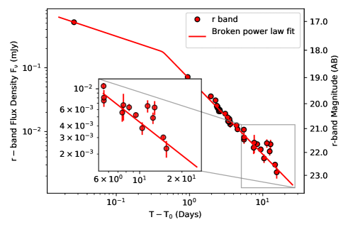
Figure 6: Broken power law fit on r-band afterglow light curve. The red dots depicts the data points in r-band and the solid line is a broken power law fit on the data. The inset shows a zoomed in version of the light curve where it shows significant deviation from power-law around $\rm{T-T_{0}}\sim 10$ d.

4.2 Broadband afterglow modelling

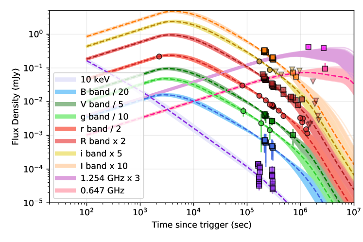
Figure 7: A multi-band light curve of GRB 210204A afterglow. The multi-band light curve of the GRB 210204A afterglow was fitted to the data using the afterglowpy package integrated with the afterglowpy with EMCEE python package for Markov Chain Monte Carlo (MCMC). Dotted lines show the best fit light curve to each band, and the light coloured band around the dotted line indicates the 16% and 84% quantiles uncertainty in the fitting.

We performed a detailed analysis of the multi-wavelength light curve of the GRB 210204A afterglow using the afterglowpy package (Ryan et al., 2020; Ahumada et al., 2021). The afterglowpy python package is an open-source computational tool to compute the afterglow light curves for the structured jet. It has the capabilities to provide light curves for arbitrary viewing angles. We integrated the afterglowpy with EMCEE (Foreman-Mackey et al., 2013) python package for Markov Chain Monte Carlo (MCMC) routine (Metropolis et al., 1953) to generate the posterior of parameters thanks to the fast light curve generation of afterglowpy. We included all radio and X-ray data in our modelling but limited our optical data to $T-T_{0}<8$ d, in order to avoid the “brightening” seen in §4.1.

Table 2: Posterior sampling using MCMC and afterglowpy

Parameter	Unit	Prior Type	Posterior	Parameter Bound
${\theta_{\mathrm{obs}}}$	rad	$\sin{({\theta}_{\mathrm{obs}})}$	$0.010^{+0.002}_{-0.002}$	[0.001, 0.8]
$\rm{log}_{10}(E_{0})$	erg	uniform	$54.06^{+0.03}_{-0.03}$	[48, 56]
$\theta_{\mathrm{core}}$	rad	uniform	$0.024^{+0.003}_{-0.002}$	[0.01, $\pi/2$]
$\log_{10}(n_{\mathrm{0}})$	cm-3	uniform	$-5.67^{+0.13}_{-0.16}$	[-6, 100]
$p$	-	uniform	$2.18^{+0.026}_{-0.026}$	[2.0001, 4]
$\epsilon_{\mathrm{e}}$	-	-	0.1	-
$\log_{10}(\epsilon_{\mathrm{B}})$	-	uniform	$-0.86^{+0.17}_{-0.15}$	[-6, 0]
$\xi$	-	-	1	-

We used the TopHat jet model in afterglowpy which performs artificial light curve modelling using a standard synchrotron fireball model. The temporal decay index $\alpha$ can be used to calculate the electron power-law index $p$ for the circum-burst medium using the closure relation $\alpha=3(p-1)/4$ (Li et al., 2020, Table 2). For constant density Inter-Stellar Medium (ISM), the optical and X-ray decays yield $p_{\mathrm{ISM,o}}\sim 2.56$ and $p_{\mathrm{ISM,x}}\sim 2.47$. On the other hand, for a wind-like medium, $\alpha=(3p-1)/4$, corresponding to unusually low values $p_{\mathrm{wind,o}}\sim 1.91$ and $p_{\mathrm{wind,x}}\sim 1.80$. We can also calculate that spectral index is $\beta\sim 0.75$ using the optical and X-ray fluxes, which in turn gives $p\sim 2.5$: consistent with the constant density ISM case. Hence, we proceed with detailed analysis assuming a constant density ISM.

Assumption of constant density medium (synchrotron Self Absorption is not important as discussed in Section 4) may cause disagreements between the model and the radio data. However, we find that the results do not significantly change whether we include radio in the fits. The MCMC routine was run to fit for angle between the jet axis and the observer ($\theta_{\mathrm{obs}}$), the total energy of the jet ($\rm{log_{10}}(E_{0})$), the half opening-angle of the jet ($\rm{\theta}_{core}$), the circumburst density ($\rm{log_{10}}(n_{0})$), the power-law index for the electron energy distribution ($p$), and the fraction of energy in electrons and the magnetic field ($\rm{log_{10}}(\epsilon_{e})$ and $\rm{log_{10}}(\epsilon_{B})$ respectively). The priors and bounds used for each parameters are shown in Table 2. We assumed a uniform distribution for $\theta_{\mathrm{core}}$, but we took the prior for the observer angle to be uniform in $\sin\theta_{\mathrm{obs}}$ to account for the uniform random orientations of sources in space (see for instance Troja et al., 2018). The exponent $p$ was assumed to be distributed uniformly in the semi-open interval $(2,4]$: implemented practically as a uniform distribution in $[2.0001,4]$. Finally, log-uniform priors were used for $\rm{E}_{0}$, $\rm{n}_{0}$, and $\epsilon_{B}$. Our preliminary fits showed that the data could not constrain $\xi$ and $\epsilon_{e}$ well, so we fixed them at nominal values of 1 (Ryan et al., 2020) and 0.1 (Panaitescu & Kumar, 2002; Gupta et al., 2021a) respectively. The source redshift was held fixed at 0.876 as discussed in §2.2.2. Inputs for the fitting were the time since an event, observation frequency, measured flux, and the flux uncertainty. afterglowpy was used to generate models for various values of the input parameters, which were then compared to the observed data. The best-fit parameters and the confidence intervals were evaluated by maximising the likelihood of the model fits to the observations.

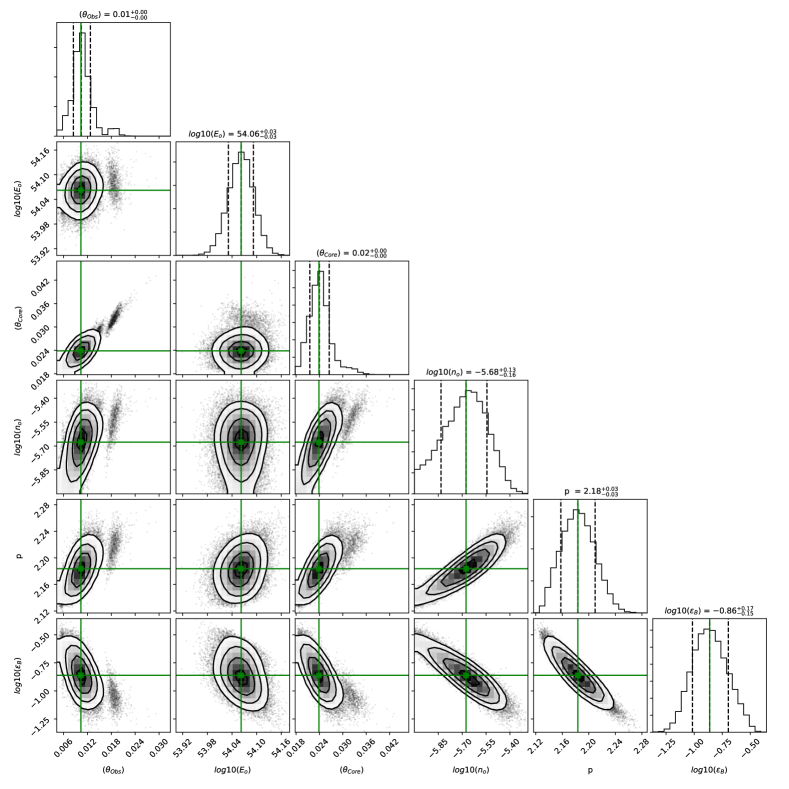
Figure 12: Posterior distribution of parameters for model fitted using afterglowpy and EMCEE. The model fit for the $\rm{\theta}_{obs}$, $\rm{\theta}_{core}$, $\rm{log_{10}}(n_{0})$, p, $\rm{log_{10}}(E_{0})$, $\rm{log_{10}}(\epsilon_{B})$ parameters. the histogram shows the 16%, 50% and 84% percentiles of probability distribution.

The one and two dimensional marginal posterior distribution resulted from the routine are shown in Figure 12. For each parameter distribution median posterior and 16% and 84% quantiles are plotted at the top of panel, which we also quote as the parameter bounds here. The model constrained the jet isotropic energy to be $10^{54.06\pm 0.03}$ ergs, consistent with typical long GRB afterglows (Wu et al., 2012). The jet structure parameter $(\rm{\theta}_{core})$ and viewing angle $(\rm{\theta}_{obs})$ were constrained at $0.024^{+0.003}_{-0.002}$ rad, $0.010\pm 0.002$ rad respectively. From the values of $\rm{\theta}_{obs}$ and $\rm{\theta}_{core}$ it is evident that the jet is seen on axis (${\theta}_{\mathrm{obs}}<{\theta}_{\mathrm{core}}$).

The best fit model generated from afterglow + MCMC routine fit is shown in Figure 7. Markers denote observed flux densities, and in several cases, the error bars are smaller than the marker size. Dashed lines show the light curves in various bands, generated using median values from parameter distribution from MCMC routine. The shaded coloured bands show 16% – 84% uncertainty regions around the median values. The fit indicates that the optical light curve would have risen at very early times, which is plausible based on the values of the synchrotron break frequencies at that time — however, we do not have any observational data to constrain this. Note that the figure shows all data, even the points at $T-T_{0}>8$ d that were excluded from the fit. We can clearly see that the re-brightening episodes have statistically significant deviations from the fit values and are indeed astrophysical in nature.

Next, we tried to estimate the break frequencies and peak time of light curve. For this we consider a spherical shock propagating in a constant density ($n$) medium. The hydrodynamic evolution of this shock can either be radiative or adiabatic, which affects the late-time light curve behaviour. Following Sari et al. (1998), if we model the flux in decaying part of light curve as $F\sim t^{-\beta}$, then the decay index can take two values in the adiabatic case: $\beta_{1}=3(p-1)/4$ or $\beta_{2}=3p/4-1/2$. Using value of $p$ from Table 2, we get $\beta_{\mathrm{1}}=0.88$, $\beta_{\mathrm{2}}=1.13$. On the other hand, $\beta\sim 3/7$ for fully radiative evolution. In §4.1, we measured this late time decay index to be $\alpha_{2}=1.18\pm 0.03$: close to the radiative $\beta_{2}$ calculated here. We conclude that the hydrodynamic shock evolution is adiabatic in nature. Hence, the equations governing shock parameters in the observers’ frame are (Sari et al., 1998):

$$\nu_{\mathrm{c}} = 2.7\times 10^{12}*(1+z)^{-1/2}\epsilon_{\mathrm{B}}^{-3/2}E_{52}^{-1/2}n_{0}^{-1}t_{\mathrm{d}}^{-1/2}~{}\mathrm{Hz}$$ (2)

$$\nu_{\mathrm{m}} = 5.1\times 10^{15}*(1+z)^{1/2}\left(\frac{p-2}{p-1}\right)^{2}\epsilon_{\mathrm{e}}^{2}\epsilon_{\mathrm{B}}^{1/2}E_{52}^{1/2}t_{\mathrm{d}}^{-3/2}~{}\mathrm{Hz}$$ (3)

$$t_{\mathrm{m}} = 2.98*(1+z)^{1/3}\left(\frac{p-2}{p-1}\right)^{4/3}\epsilon_{\mathrm{e}}^{4/3}\epsilon_{\mathrm{B}}^{1/3}E_{52}^{1/3}\nu_{\mathrm{15}}^{-2/3}~{}\mathrm{days}$$ (4)

$$t_{\mathrm{0}} = 1.89\times 10^{3}*(1+z)\left(\frac{p-2}{p-1}\right)^{2}\epsilon_{\mathrm{e}}^{2}\epsilon_{\mathrm{B}}^{2}E_{52}n_{0}~{}\mathrm{days}$$ (5)

Here, $t_{d}$ is time in days since the trigger, $n_{0}$ is the Interstellar Medium (ISM) density in units of $\mathrm{cm}^{-3}$, $E_{52}=E_{0}/10^{52}$ ergs, $\nu_{\mathrm{15}}=\nu/10^{15}~{}\mathrm{Hz}$ and $t_{\mathrm{m}}$ is peak time. At $t=t_{0}$, equation 2 and 3 satisfy $\nu_{0}=\nu_{c}(t_{0})=\nu_{m}(t_{0})$ (Sari et al., 1998) where $\nu_{0}$ is called critical frequency. $t=t_{0}$ is the time at which the ejecta transitions from fast cooling to slow cooling phase. Using best–fit values from Table 2, Equation 5 yields $t_{0}\sim 3.85\times 10^{-6}$ days — showing that GRB 210204A transitioned to the slow cooling phase at very early times. This in turn gives a “critical frequency” $\nu_{\mathrm{0}}=2.21\times 10^{21}$ Hz which lies in $\gamma-\mathrm{ray}$ frequency range as shown by horizontal black dashed line in Figure 8, suggesting that the light curve shown in Figure 7 is a low-frequency light curve (Sari et al., 1998). The optical light curve will peak when the synchrotron frequency ($\nu_{\mathrm{m}}$) passes through optical bands at $t_{\mathrm{m}}=0.055~{}\mathrm{days}=4.75\times 10^{3}~{}\mathrm{s}$, in agreement with the afterglowpy fits for GRB 210204A shown in Figure 7. However, we lack sufficient early-time data to constrain such a rise. On the other hand, the cooling frequency at $\sim 1$ day $\nu_{\mathrm{c,t=1}}=1.68\times 10^{18}$ Hz, lies in X-ray bands ($E\sim 7$ keV) which accounts for different decay in X-ray and optical bands at early times.

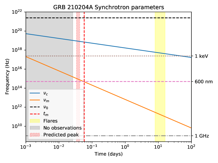
Figure 8: The interplay of break frequencies with time. The blue and orange solid line represents variation of $\nu_{c}$ and $\nu_{m}$ respectively with time. $\nu_{m}$ passes through the optical frequency (horizontal magenta dashed line) at $t=t_{m}$ (vertical dashed red line). Grey shaded region shows epochs where no observations were made. The yellow shaded region depicts flaring event. The narrow light red region at $\sim 3\times 10^{3}$ s is where the light curve is predicted to be peaked through afterglowpy modelling of light curve.

4.3 Quantifying the re-brightening

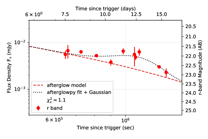
(a) 1D Gaussian fit

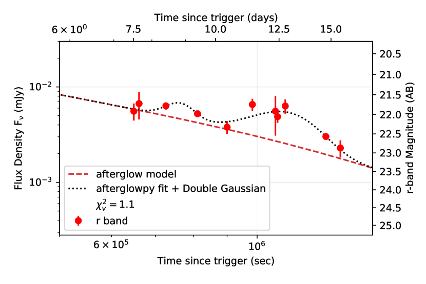
(b) 1D Double Gaussian fit

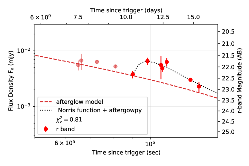
(c) Norris function fit

Figure 9: Late-time excessive emission fitting with various models. a) A simple Gaussian fitting to the peak. b) A double Gaussian fit to the late-time variability. c) Norris function fitted on the two peaks for flaring. The solid dark markers shows the data used for fitting for a particular function.

Armed with our best-fit model for the afterglow, we revisit the re-brightening episode discussed in §4.1. Figure 6 shows that these episodes occur only for a few nights, after which the data seem to return to the original power-law decay. We verified this starting with detailed quality checks on our data in this time range: including visual inspection, checking the stability of light curves of nearby stars, and re-checking the zero points. We find that the photometric measurements are robust, and the data indeed are brighter than the level expected from the afterglow model.

Next, we fit simple models to these episodes to measure their properties. In all fits, we use the nominal afterglow light curve from §4.2 as a “background” (red dashed lines in Figure 9), and add various “flare” models to this. We start with a simple Gaussian in flux density space: $F=F_{0}\exp[(t-t_{\mathrm{peak}})^{2}/(2\sigma^{2})]$, where $F_{0}$ is the peak flux density, $t_{\mathrm{peak}}$ is the time of the peak, measured from the GRB $T_{0}$, and $\sigma$ is the duration parameter. We obtain best-fit values as $F_{0}=0.0024\pm 0.0006$ mJy, $t_{\mathrm{peak}}=(105\pm 3)\times 10^{4}~{}\mathrm{s}=12.1\pm 0.3$ d and $\sigma=(17.2\pm 3.3)\times 10^{4}~{}\mathrm{s}=2.0\pm 0.4$ d. This corresponds to an overall fluence of $7.87\times 10^{-10}$ $\mathrm{erg~{}cm}^{-2}$. However, the quality of the fit is not very good (Figure 9a), as the photometry is close to the predicted light curve till $\sim 10$ days, and rises strongly after that. Hence, we fit two gaussians to the data, as shown in Figure 9b. The best-fit parameters for the first peak are $F_{1}=0.002\pm 0.011$ mJy, $t_{\mathrm{peak,1}}=76\pm 6)\times 10^{4}~{}\mathrm{s}=8.8\pm 0.7$ d and $\sigma_{1}=(3.7\pm 1.6)\times 10^{4}~{}\mathrm{s}=0.4\pm 0.2$ d, while the best-fit parameters for the more pronounced second peak are $F_{2}=0.0029\pm 0.0006$ mJy, $t_{\mathrm{peak,2}}=(110\pm 3)\times 10^{4}~{}\mathrm{s}=12.7\pm 0.3$ d and $\sigma_{2}=(12.0\pm 2)\times 10^{4}~{}\mathrm{s}=1.4\pm 0.2$ d. The total fluence of the two peaks is $5.73\times 10^{-10}$ $\mathrm{erg~{}cm}^{-2}$ and $9.83\times 10^{-10}$ $\mathrm{erg~{}cm}^{-2}$ respectively.

Any re-brightening or flaring episode is likely to have an asymmetric profile with a faster rise and slower decline that is not appropriately modelled by a Gaussian function. Hence, we fit them with a more plausible model, the Norris function (Norris et al., 2005). The intensity of the flare is modelled as

$$I(t)=A\lambda\exp\left(-\frac{\tau_{1}}{(t-t_{i})}-\frac{(t-t_{i})}{\tau_{2}}\right)$$ (6)

where $t_{i}$ is the pulse start time, and the equation holds for $t>t_{i}$. The parameters $\tau_{1}$ and $\tau_{2}$ are associated with the rising and decaying phases of the pulse, but are not directly the rise and decay timescales. The burst intensity is given by the parameter $A\lambda$, where $\lambda=\exp(2\sqrt{\tau_{1}/\tau_{2}})$. We ignore the weaker first episode here, but find that the second episode is fit well by Equation 6. The burst “start time” is $t_{i}=88\pm 3\times 10^{4}$. The peak time is $t_{\mathrm{peak}}=t_{i}+\sqrt{\tau_{1}/\tau_{2}}=(9.9\pm 2.4)\times 10^{5}~{}\mathrm{s}=11.5\pm 2.7$ d — consistent with, but bit sooner than, the values obtained from the double Gaussian fit. The width of the pulse is $w=\tau_{2}(1+4\sqrt{\tau_{1}/\tau_{2}})=(3.2\pm 1.4)\times 10^{5}~{}\mathrm{s}=3.7\pm 1.6$ d. Under this model, the fluence of the pulse is $1.48\times 10^{-9}$ $\mathrm{erg~{}cm}^{-2}$. For comparison, the total fluence of the underlying afterglow model in the same duration is $1.85\times 10^{-9}$ $\mathrm{erg~{}cm}^{-2}$.

In summary, we see evidence for two re-brightening episodes in the afterglow, at about 8.8 and 12.7 days after the burst. The second episode is the more significant, with $\Delta t/t$ values $\sim 0.25$ and 0.33, and $\Delta F/F\sim$ 1.14 and 1.07 for the double-Gaussian and Norris models, respectively.

5 Discussion

The afterglow of GRB 210204A is quite typical in early times, following a broken power-law behaviour (§4.1) that is modelled well with as a standard afterglow with afterglowpy (§4.2). The late–time deviations from a smooth decay (§4.3) can arise from a variety of reasons in long GRB afterglows.

A common cause for a re–brightening is the appearance of the supernova associated with the GRB (§5.1). Flaring may also occur due to patchy shells in the jet (§5.2) or interaction of the jet with inhomogeneities the ISM (§5.3). Various shocks can also cause flaring — for instance a reverse shock in the ejecta (§5.4) or a collision of two forward shocks (§5.5). Delayed activity by the central engine may manifest directly as flaring (§5.6), or interactions between a delayed jet and a cocoon (§5.7), or may refresh the forward shock (§5.8).

We discuss these in detail below, testing each probable cause for the re-brightening in GRB 210204A.

5.1 Supernova

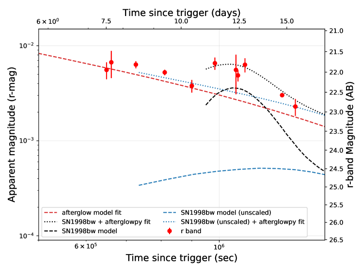
Figure 10: K-corrected SN 1998bw light curve plotted with the excessive emission in GRB 210204A. The dashed red line shows the afterglow model, while the dotted black line shows the afterglow and scaled supernova combined model plotted in the observers’ frame. The scaled supernova-only model (black dashed line) was obtained by scaling SN 1998bw model (blue dashed line) flux up by 7$\times$, stretched to be eight times faster (shorter) than actual, and shifted in time such that the supernova started six days after the GRB. The unscaled SN 1998bw model fitted over the afterglowpy model is shown with blue dotted lines for comparison. This is an unreasonable set of parameters; thus, a supernova cannot explain the re-brightening.

In many long GRBs, the very late-time supernova (SN) bump follows the afterglow emission indicating the collapsar origin for the burst (Galama et al., 1998; de Ugarte Postigo et al., 2017; Roy, 2021). To test this possibility, we used the light curve of the prototypical SN 1998bw to compare this excessive emission. As a starting point, we referred to SN 1998bw data from Clocchiatti et al. (2011) and applied a K-correction (Bloom et al., 2001) using redshift of GRB 210204A. Using cubic splines, we interpolated the fluxes into the observed $r$ band values. A continuous light curve was created using cubic interpolation on these values. The resulted light curves were then further scaled in flux (k), stretch in evolution (s) and shifted in time (S_t) to fit GRB 210204A light curve. The SN1988bw model light curve overplotted with the GRB 210204A data is shown in Figure 10. Typical GRB supernovae have absolute magnitudes in the range $-17.5$ to $-20$ with median value $\sim-19.5$ mag (Richardson, 2009), and peak about $\sim 20$ days after the GRB in the rest frame. At the redshift of GRB 210204A, it would correspond to an apparent magnitude of 24.6, peaking 38 days after the trigger in the observers’ frame. We note that this is the bolometric magnitude, while our observations are in the r band — corresponding to the rest frame u band. Thus, the expected supernova will be even fainter due to the finite bandwidth and possible extinction. The observed episodes occur much sooner and are much brighter than these values.

Thus, to explain the re-brightening seen in GRB 210204A as a supernova similar to SN 1998bw, the SNe light curve has to be made shorter by a factor of 8 ($s=1/8$), the flux has to be made brighter by a factor of $k\sim$ 7, and the supernova onset has to be delayed by $\sim 6$ days to get a reasonable fit. These parameters — in particular the shorter timescale and delayed onset of the supernova — are quite unphysical, and we do not find any acceptable values that can match the light curve. Hence we conclude that the re-brightening is not associated with a supernova.

5.2 Patchy shell model

The patchy shell model attributes the variability in GRB afterglows to random angular fluctuations in the energy of the relativistic jet (Nakar & Oren, 2004). However, such variations are expected at earlier times when there are causally disconnected regions within the jet opening angle. However, the variability caused by this mechanism has timescales $\Delta t\gtrsim t$, (Nakar & Oren, 2004; Ioka et al., 2005), inconsistent with our measurements. Therefore, we rule out the patchy shell model as a potential cause for the re-brightening seen in GRB 210204A.

5.3 Variations due to fluctuation in ISM density

Ambient density fluctuations can account for late-time variability in GRB afterglows (Wang & Loeb, 2000; Lazzati et al., 2002; Ioka et al., 2005). Such inhomogeneities are primarily caused due to winds from the progenitor or due to turbulence in the ambient medium. Ioka et al. (2005) put an upper limit on flux variation due to inhomogeneities in the ambient medium of standard afterglows for on–axis jets:

$$\frac{\Delta F_{\nu}}{F_{\nu}}\leq\frac{4}{5}f_{\mathrm{c}}^{-1}\frac{F}{\nu F_{\nu}}\frac{\Delta t}{t}$$ (7)

Here $f_{\mathrm{c}}\sim(\nu_{\mathrm{m}}/\nu_{\mathrm{c}})^{(p-2)/2}$. The light curve of GRB 210204A is governed by slow cooling, with optical-band frequencies satisfying $\nu_{\mathrm{m}}<\nu_{opt}<\nu_{\mathrm{c}}$ criteria at time of excessive emission ($t\sim 12$ days) seen in GRB 210204A light curve (see §4.2). For such cases the $F/\nu F_{\nu}\sim(\nu/\nu_{m})^{(p-3)/2}$ (Ioka et al., 2005). This suggests $\frac{\Delta F_{\nu}}{F_{\nu}}\leq 0.14$, which is significantly lower than actual value of 1.07 — 1.14 (§4.3). Further, Nakar & Piran (2003) show that assuming a spherically symmetric ISM profiles, any flaring from such interactions will have $\Delta t/t>1$ which is also inconsistent with our measurements. Thus we rule out fluctuations in ambient density as possible origin of flare.

5.4 Reverse-Shock emission in ejecta medium

The interaction of blast-wave and circumburst medium results in two shock waves: the forward shock moving towards circumburst medium and a reverse shock moving back into ejecta itself. The reverse shock could produce an optical peak in the observed optical light curve at early times (Kobayashi & Zhang, 2003; Gao et al., 2015; Greiner et al., 2009). Reverse shock is expected to rise rapidly in constant density medium under thin shell approximation case ($\alpha_{\mathrm{rise}}=3p-3/2$, where $p$ is the power-law index of the electron distribution), and decline, with $\alpha_{\mathrm{decline}}=-(27\mathrm{p}+7)/35$ (Kobayashi, 2000; Greiner et al., 2009). The canonical range of electron distribution index (p) = $2.2-2.5$ (Greiner et al., 2009). The estimated rising and decaying temporal indices of the optical flare are $\sim 6.2$ and $\sim 3.4$, respectively. This implies p $\sim 2.56$ and $4.15$ before and after the peak of the flare, respectively. The inconsistent values of p during the rising and decaying part indicate that the flare is not a result of external reverse shock decay. Moreover, the observed peak time occurs at t_peak = (9.90 $\pm$ 2.31) $\times$ 10⁵ s post burst, far later than the $10^{3-4}$ s delays expected from flares caused by the reverse shock component in optical bands (Kobayashi & Zhang, 2003; Uhm & Beloborodov, 2007).

5.5 Collision of two forward shocks

An external collision between shells of GRB can produce flaring on top of afterglow decay (Perna et al., 2006; Zhang et al., 2006; Burrows et al., 2005b; Chincarini et al., 2007). The time and amplitude and duration of such flares vary among GRBs, depending upon the interaction time, Lorentz factor ($\Gamma$) and the energy $\rm{E}_{iso}$ of the colliding shells. Vlasis et al. (2011) discuss a scenario where a shell with a lower $\Gamma$ is ejected first from the central engine, followed by a shell with a higher $\Gamma$. The first shell decelerates further as it interacts with the interstellar medium, and the second (faster) shell can catch up and ram into the first shell, producing optical flares. For typical GRBs, flares created by such a mechanism should have $\Delta t/t~{}\sim 1$ where $\Delta t$ is the full width at half maximum of the flare, and $t$ is the time at which the flare peaks. We also expect $\Delta F/F~{}\sim$ 2-5, where $F$ is the flux of the afterglow and $\Delta F$ is the excess brightening caused by the flare (Vlasis et al., 2011).

The measured $\Delta t/t$ and $\Delta F/F$ values (§4.3) are smaller than the predictions of Vlasis et al. (2011). Thus, we conclude that it is unlikely that collisions between forward shocks caused the late time flaring.

5.6 Late-time flaring emission from central engine

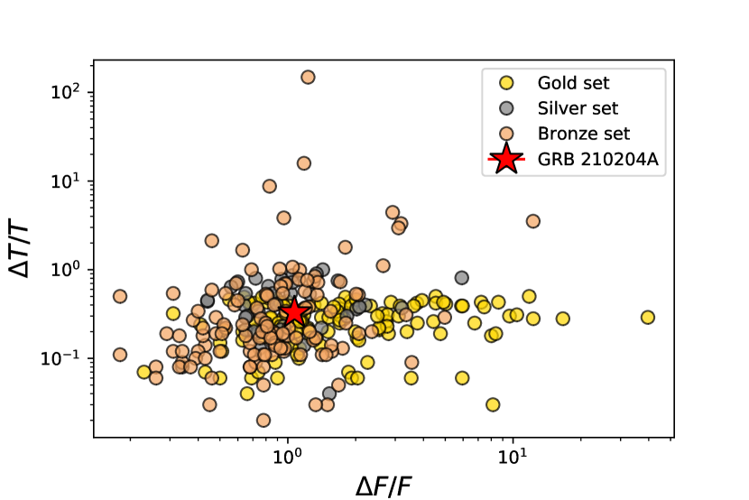
(a)

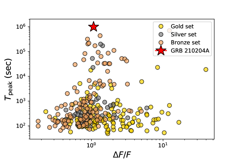
(b)

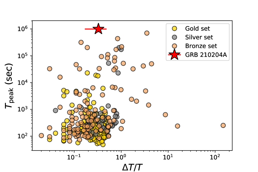
(c)

Figure 11: Comparison of flaring properties of GRB210204A with GRB flares published in Swenson & Roming (2014). The gold, silver and bronze sets are shown by respective colors. GRB 210204A is depicted with red star symbol, with the limits of the error bar indicating the two $\Delta t$ values measured in §4.3. The flare is very similar to other flares in terms of $\Delta F/F$ and $\Delta t/t$, but occurs later than any of the flares in the Swenson & Roming (2014) data set.

Flaring activity is fairly common in GRB afterglows — seen in more than 50% of the GRBs in X-rays (O’Brien et al., 2006) and $\sim 33\%$ of GRB light curves in optical (Swenson et al., 2013). Due to the very limited amount of X-ray data for GRB 210204A, we focus on r-band optical observations here — in particular, the second re-brightening episode. Flaring in afterglows may be caused by external shocks caused when the jet interacts with density bumps in the interstellar medium (which is discussed in §5.3), or internal shocks from a central engine that is still active, which we discuss here. Indeed, the presence of the three episodes in the prompt emission of GRB 210204A is itself an encouraging sign that the central engine is capable of injecting energy multiple times. Such central engine activity itself is typically ascribed to two scenarios. The first possibility is a long-lived magnetar, active to late times (Usov, 1994; Dai & Lu, 1998; Rees & Mészáros, 2000). The other possibility is the delayed formation of a black hole in a collapsar, with an accretion disk that may feed matter to the black hole for days (MacFadyen et al., 2001).

Flares are typically characterised by the flaring timescale as compared to the delay time and the fractional increase in flux (Ioka et al., 2005). From §4.3, we have $\Delta t/t\sim 0.25$ and $\Delta F/F\sim 1.14$. These values are consistent with the classical flaring criteria $\Delta t/t\leq 1$ (Swenson et al., 2013; Swenson & Roming, 2014). Next, we compare the properties of the flare with the Swenson et al. (2013) sample. Figure 11(a) shows that the flare is similar to other flares in the duration and flux ratios. What sets it apart is the peak time (Figures 11(c)). However, this may be an observational bias, as late-time observations by UVOT or other telescopes are not as common.

Based on the long delay after the GRB, the flares are unlikely to be directly associated with late-time central engine activity. However, we cannot fully rule out this possibility due to the lack of multi-wavelength data.

5.7 Interaction of a delayed jet with a cocoon

The passage of the prompt jet through the stellar envelope creates a cocoon of material (Nakar & Piran, 2017). As the main jet subsides, the cocoon quickly gets filled in due to transverse spreading, presenting a barrier to any delayed jet components like ones discussed in §5.6. Shen et al. (2010) argue that the interaction of such late jet components with the ejecta can cause broadband flaring. Such flares have $\Delta t/t<0.5$, and the flux can vary drastically depending on the system parameters. For instance, they predict that for a GRB with redshift 2, the optical $V$-band magnitude for such a flare may be anywhere between 11.5–29, comfortably encompassing the values observed for our $z=0.876$ case. However, the resultant flares are expected to occur at earlier times: typically starting at 100 s after the burst, but possibly up to 10⁴–10⁵ s after the event. The flaring in GRB 210204A occurs an order of magnitude later in time, and thus is not any more likely to be caused by interactions between a delayed jet and a cocoon than any other causes of late engine activity discussed in §5.6.

5.8 Refreshed shock

The late-time brightening in the optical light curve could also have originated from a forward shock that is refreshed by late-time energy injection from the central engine (Rees & Mészáros, 1998; Panaitescu et al., 1998). Such a refreshed shock scenario has been used to explain the observed re-brightening in the optical light curves of GRB 030329 (Granot et al., 2003) and GRB 120326A (Melandri et al., 2014). Consider a standard forward shock model where the bulk Lorentz factor of the ejecta is not constant but has a range of values. Faster moving shells with higher Lorentz factors ($\Gamma_{\rm fast}\geq$ 100) interact with the surrounding medium first and are slowed down. Slower moving shells ($\Gamma_{\rm slow}\sim$ 10) catch up with these decelerated shells at late times, injecting energy into the shock and increasing the emission. Genet et al. (2006) derived the formula for the collision time of two shells (one moving with $\Gamma_{\rm slow}\sim$ 10 and other moving with $\Gamma_{\rm fast}\geq$ 100) considering the simple assumption (see equation 8),

$$t_{\rm shock}\approx 1.66\times E_{\rm\gamma,iso,53}^{1/3}~{}n_{0}^{-1/3}~{}\Gamma_{\rm slow,10}^{-8/3}~{}~{}~{}~{}{\rm days}$$ (8)

In this equation, $E_{\rm\gamma,iso,53}$ denotes $E_{\rm\gamma,iso}$/10⁵³ in erg, n₀ is the density for a constant medium which we obtained from broadband afterglow modelling, $\Gamma_{\rm slow,10}$ is the bulk Lorentz factor of slow moving shell in the unit of 10. Following the above equation, we calculated the Lorentz factor of the slow moving shell for GRB 210204A at the time of optical brightening. We take $t_{\rm shock}\sim 12.7$ days from our two-Gaussian fit (§4.3), and substitute $E_{\rm\gamma,iso,53}=10^{1.06}$ erg, n${}_{0}=10^{-5.65}~{}\mathrm{cm}^{-3}$ from Table 2 to get $\Gamma_{\rm slow}\sim 32$.

For flares caused by refreshed shocks, we expect $\Delta t/t>1/4$, broadly consistent with the values measured in §4.3. Thus, a refreshed shock scenario is a plausible explanation for these flares.

6 Summary and Conclusion

We presented a detailed analysis of the prompt emission and afterglow of GRB 210204A. The prompt emission consists of three distinct emission episodes in Fermi-GBM data, separated by quiescent phases. Spectral analysis of the third and brightest episode shows the presence of a thermal component at low energies, adding a member to the small but growing class of GRBs with thermal components. We also find that GRB 210204A (full interval), as well as the individual pulses, are consistent with the Amati relation.

GRB 210204A stands out by having the most delayed flaring activity ever detected in GRBs. A flare is detected 8.8 days after the burst, followed by a stronger flare at 12.7 days. We analyse a multitude of possible causes for such flaring and rule out most of them. We conclude that the flaring is likely caused by late-time activity in the central engine — manifesting either as flares caused due to internal shocks, the interaction of a delayed jet with a cocoon or by refreshing a forward shock.

Such late-time data are not available for most GRBs. It is plausible that more GRBs exhibit such late time flaring activity, but the sample suffers severally from observational biases. This underscores the need for a systematic follow-up program for GRB afterglows. We have undertaken such a program with the GROWTH-India telescope to probe afterglow features in detail.

Data Availability

All data used in this article have been included in a tabular format within the article.

Appendix A Additional figures from afterglow fits

Table 3: Log of our photometry observations of the optical afterglow of GRB 210204A, taken with various ground-based telescopes.

JD	T-T0 (sec)	Filter	Magnitude	Telescope/Instrument
2459248.74875	-88273.15200	r	> 20.87	P48$+$ZTF
2459248.76859	-86558.15520	g	> 21.34	P48$+$ZTF
2459248.83259	-81029.15136	i	> 20.22	P48$+$ZTF
2459249.71868	-4471.14816	g	> 18.74	P48$+$ZTF
2459249.79662	2262.85056	r	17.16 $\pm$ 0.03	P48$+$ZTF
2459250.71466	81581.85216	r	19.31 $\pm$ 0.06	P48$+$ZTF
2459250.75523	85086.84960	g	19.75 $\pm$ 0.08	P48$+$ZTF
2459251.72700	169047.84672	r	19.99 $\pm$ 0.08	P48$+$ZTF
2459251.73331	169592.84928	i	19.71 $\pm$ 0.10	P48$+$ZTF
2459251.89443	183513.85056	g	20.62 $\pm$ 0.2	P48$+$ZTF
2459253.72924	342041.84928	i	> 19.80	P48$+$ZTF
2459254.82180	436438.85184	i	> 20.70	P48$+$ZTF
2459257.80761	694412.84448	i	> 20.00	P48 + ZTF
2459260.82290	954933.84864	i	> 19.70	P48$+$ZTF
2459252.35734	223509.45600	r	20.55 $\pm$ 0.03	GIT
2459253.20464	296715.74400	r	20.89 $\pm$ 0.03	GIT
2459254.29448	390877.92000	r	21.31 $\pm$ 0.04	GIT
2459255.32039	479516.97600	r	21.72 $\pm$ 0.05	GIT
2459266.24093	1423051.63200	r	> 22.39	GIT
2459267.194	1505396.44800	r	> 22.30	GIT
2459271.19364	1850965.34400	r	> 20.81	GIT
2459272.22723	1940267.52000	r	> 20.57	GIT
2459274.17682	2108712.09600	r	> 21.69	GIT
2459275.17860	2195266.32000	r	> 22.0	GIT
2459252.13277	204106.17600	R	20.17 $\pm$ 0.05	HCT
2459252.13753	204517.44000	R	20.16 $\pm$ 0.05	HCT
2459252.14045	204769.72800	R	20.15 $\pm$ 0.03	HCT
2459252.14231	204930.43200	R	20.20 $\pm$ 0.06	HCT
2459252.15787	206274.81600	I	19.77 $\pm$ 0.06	HCT
2459252.16027	206482.17600	I	19.69 $\pm$ 0.04	HCT
2459252.16265	206687.80800	I	19.74 $\pm$ 0.06	HCT
2459252.16742	207099.93600	I	19.78 $\pm$ 0.06	HCT
2459253.2722	302552.92800	R	20.67 $\pm$ 0.05	HCT
2459253.28418	303588.00000	I	20.17 $\pm$ 0.04	HCT
2459258.08132	718060.89600	I	21.30 $\pm$ 0.20	HCT
2459258.10539	720140.54400	V	22.14 $\pm$ 0.11	HCT
2459260.18751	900035.71200	R	22.22 $\pm$ 0.15	HCT
2459252.18709	208799.84822	R	20.19 $\pm$ 0.03	DFOT
2459259.15934	811201.82400	R	21.86 $\pm$ 0.07	DFOT
2459259.34474	827220.38400	I	21.60 $\pm$ 0.10	DFOT
2459252.18877	208944.96221	R	20.22 $\pm$ 0.04	DOT
2459252.19235	209255.02675	R	20.24 $\pm$ 0.04	DOT
2459252.19528	209508.05174	I	19.64 $\pm$ 0.05	DOT
2459252.19748	209698.10842	I	19.68 $\pm$ 0.05	DOT
2459252.20512	210359.26022	V	20.62 $\pm$ 0.05	DOT
2459252.20909	210701.33424	B	21.18 $\pm$ 0.09	DOT
2459252.21269	211011.89040	B	21.30 $\pm$ 0.06	DOT
2459252.21269	211011.89213	B	21.18 $\pm$ 0.08	DOT
2459252.21669	211357.47053	B	21.13 $\pm$ 0.09	DOT
2459252.26456	215493.34522	I	19.67 $\pm$ 0.04	DOT
2459252.26845	215829.42480	R	20.29 $\pm$ 0.05	DOT
2459252.27239	216169.98163	V	20.69 $\pm$ 0.06	DOT
2459252.27631	216509.06707	B	21.13 $\pm$ 0.08	DOT
2459252.27990	216819.10569	B	21.20 $\pm$ 0.09	DOT
2459252.28421	217191.69187	I	19.66 $\pm$ 0.04	DOT
2459252.28808	217525.78684	R	20.37 $\pm$ 0.06	DOT
2459252.29246	217903.83609	V	20.69 $\pm$ 0.06	DOT
2459252.35158	223012.44518	I	19.81 $\pm$ 0.07	DOT
2459252.35554	223354.01980	R	20.34 $\pm$ 0.07	DOT
2459252.35939	223687.06848	V	20.72 $\pm$ 0.08	DOT
2459252.36324	224019.63072	B	21.29 $\pm$ 0.12	DOT
2459252.36688	224333.71804	B	21.31 $\pm$ 0.12	DOT
2459252.37481	225019.35734	I	19.78 $\pm$ 0.07	DOT
2459252.37847	225335.42669	I	19.81 $\pm$ 0.07	DOT
2459252.38265	225696.52339	R	20.37 $\pm$ 0.08	DOT
2459253.12825	290116.63123	R	20.76 $\pm$ 0.05	DOT
2459253.13132	290381.68829	I	20.20 $\pm$ 0.05	DOT
2459253.13448	290654.74858	V	21.09 $\pm$ 0.05	DOT
2459253.13721	290890.30608	B	21.59 $\pm$ 0.09	DOT
2459253.13964	291100.84646	B	21.57 $\pm$ 0.09	DOT
2459253.17108	293816.41402	I	20.25 $\pm$ 0.05	DOT
2459253.17355	294030.45274	R	20.76 $\pm$ 0.05	DOT
2459253.17646	294281.51472	V	21.11 $\pm$ 0.05	DOT
2459253.23432	299280.58329	I	20.22 $\pm$ 0.05	DOT
2459253.23678	299493.63014	R	20.79 $\pm$ 0.06	DOT
2459253.23947	299725.66166	R	20.79 $\pm$ 0.12	DOT
2459253.24264	299999.70950	B	21.58 $\pm$ 0.08	DOT
2459253.28455	303620.97456	I	20.33 $\pm$ 0.11	DOT
2459253.28769	303892.56432	R	20.78 $\pm$ 0.12	DOT
2459253.29160	304230.13776	B	21.70 $\pm$ 0.09	DOT
2459253.35684	309866.34932	I	20.34 $\pm$ 0.07	DOT
2459253.35955	310100.86915	R	20.88 $\pm$ 0.06	DOT
2459253.36224	310332.94905	R	20.87 $\pm$ 0.13	DOT
2459262.54515	1103736.61238	r	21.90 $\pm$ 0.17	DOT
2459264.50267	1272865.95763	r	22.70 $\pm$ 0.05	DOT
2459265.27083	1339234.84771	r	23.00 $\pm$ 0.20	DOT
2459265.43097	1353071.30659	r	> 22.59	DOT
2459266.45952	1441938.10176	r	> 21.44	DOT
2459267.38564	1521954.81360	r	> 21.13	DOT
2459269.53000	1707227.09337	r	> 19.14	DOT

Table 4: Photometry table of the optical afterglow of GRB 210204A, data obtained from various reported GCNs.

JD	T-T0 (sec)	Filter	Magnitude	Instrument	Reference
2459252.0362	195764	R	19.94 $\pm$ 0.09	AZT-33IK	29417
2459252.2179	211462	R	20.1 $\pm$ 0.04	AS-32	29417
2459252.8472	265835	g	21.10 $\pm$ 0.10	LBT	29433
2459252.8472	265835	r	20.70 $\pm$ 0.10	LBT	29433
2459252.8472	265835	i	20.40 $\pm$ 0.10	LBT	29433
2459252.8472	265835	z	20.2 $\pm$ 0.10	LBT	29433
2459253.0930	287073	R	20.61 $\pm$ 0.04	AZT-33IK	29438
2459254.1607	379326	R	20.92 $\pm$ 0.05	AZT-33IK	29438
2459255.2961	477422	R	21.09 $\pm$ 0.08	DFOT	29490
2459255.3265	480047	R	21.4 $\pm$ 0.20	ZTSh	29499
2459257.2800	648835	R	21.8 $\pm$ 0.20	AS-32	29499
2459257.4186	660802	R	21.6 $\pm$ 0.30	AS-32	29499
2459258.1744	726104	R	21.66 $\pm$ 0.09	AZT-33IK	29520
2459261.1528	983436	r	21.86 $\pm$ 0.15	AZT-20	29520
2459262.1110	1066228	R	21.8 $\pm$ 0.40	AZT-33IK	29520
2459262.2063	1074461	r	22.18 $\pm$ 0.14	AZT-20	29520

Table 5: Log of X-ray observations of the X-ray afterglow of GRB 210204A taken using SwiftXRT in 10 keV band. This data uses a absorption of $0.61\times 10^{22}\rm{cm}^{-2}$ at $z$ = 0.876.

JD	T-T0 (sec)	Photon Index	Flux Density ($\mu$Jy)
2459251.634	161000.965	$1.61^{+0.29}_{-0.22}$	140.99 $\pm$ 31.98
2459251.636	161214.462	$1.62^{+0.28}_{-0.21}$	124.61 $\pm$ 28.42
2459251.640	161501.848	$1.65^{+0.27}_{-0.20}$	138.95 $\pm$ 24.97
2459251.702	166845.863	$2.11^{+0.24}_{-0.19}$	42.26 $\pm$ 9.79
2459251.704	167087.251	$2.13^{+0.25}_{-0.20}$	35.41 $\pm$ 9.41
2459251.706	167273.799	$2.15^{+0.25}_{-0.20}$	51.94 $\pm$ 11.80
2459251.708	167449.688	$2.14^{+0.25}_{-0.20}$	59.20 $\pm$ 13.42
2459251.712	167726.371	$2.11^{+0.24}_{-0.19}$	32.05 $\pm$ 8.73
2459251.767	172498.443	$1.64^{+0.29}_{-0.22}$	118.14 $\pm$ 26.65
2459251.769	172708.123	$1.62^{+0.30}_{-0.23}$	107.96 $\pm$ 27.21
2459251.773	173048.102	$1.61^{+0.30}_{-0.23}$	80.00 $\pm$ 17.04
2459253.174	294064.238	$1.46^{+0.30}_{-0.22}$	63.53 $\pm$ 16.86
2459253.178	294390.208	$1.46^{+0.30}_{-0.22}$	96.35 $\pm$ 25.20
2459253.182	294775.487	$1.48^{+0.29}_{-0.22}$	66.52 $\pm$ 17.42
2459253.187	295152.375	$1.52^{+0.27}_{-0.20}$	61.49 $\pm$ 15.55
2459253.239	299664.401	$2.0^{+0.29}_{-0.21}$	35.88 $\pm$ 9.36
2459253.243	300009.566	$2.04^{+0.30}_{-0.23}$	25.27 $\pm$ 6.62
2459253.247	300337.201	$2.08^{+0.32}_{-0.24}$	42.59 $\pm$ 11.11
2459253.250	300677.495	$2.11^{+0.34}_{-0.26}$	27.84 $\pm$ 7.04

Table 6: Log of radio data for the radio afterglow of GRB 210204A taken using uGMRT.

JD	T-T0 (sec)	Energy-Band	Flux ($\mu$Jy)
2459266.06	1402272.00	1254.6 GHz	140 $\pm$ 22
2459281.09	2706011.71	1254.6 GHz	130 $\pm$ 20
2459283.06	2876272.416	647.8 GHz	95 $\pm$ 45

References

- Ahumada et al. (2021) Ahumada T., et al., 2021, Nature Astronomy, 5, 917
- Alam et al. (2015) Alam S., et al., 2015, ApJS, 219, 12
- Amati (2006) Amati L., 2006, MNRAS, 372, 233
- Andreoni et al. (2021) Andreoni I., et al., 2021, ApJ, 918, 63
- Arnaud (1996) Arnaud K. A., 1996, in Jacoby G. H., Barnes J., eds, Astronomical Society of the Pacific Conference Series Vol. 101, Astronomical Data Analysis Software and Systems V. p. 17
- Band et al. (1993) Band D., et al., 1993, ApJ, 413, 281
- Basak & Rao (2013) Basak R., Rao A. R., 2013, MNRAS, 436, 3082
- Bellm (2014) Bellm E., 2014, in Wozniak P. R., Graham M. J., Mahabal A. A., Seaman R., eds, The Third Hot-wiring the Transient Universe Workshop. pp 27–33 (arXiv:1410.8185)
- Bertin (2011) Bertin E., 2011, in Evans I. N., Accomazzi A., Mink D. J., Rots A. H., eds, Astronomical Society of the Pacific Conference Series Vol. 442, Astronomical Data Analysis Software and Systems XX. p. 435
- Bertin & Arnouts (1996) Bertin E., Arnouts S., 1996, A&AS, 117, 393
- Bertin et al. (2002) Bertin E., Mellier Y., Radovich M., Missonnier G., Didelon P., Morin B., 2002, in Bohlender D. A., Durand D., Handley T. H., eds, Astronomical Society of the Pacific Conference Series Vol. 281, Astronomical Data Analysis Software and Systems XI. p. 228
- Bhalerao et al. (2017) Bhalerao V., et al., 2017, Journal of Astrophysics and Astronomy, 38, 31
- Bloom et al. (2001) Bloom J. S., Frail D. A., Sari R., 2001, AJ, 121, 2879
- Burgess et al. (2020) Burgess J. M., Bégué D., Greiner J., Giannios D., Bacelj A., Berlato F., 2020, Nature Astronomy, 4, 174
- Burrows et al. (2005a) Burrows D. N., et al., 2005a, Space Sci. Rev., 120, 165
- Burrows et al. (2005b) Burrows D. N., et al., 2005b, Science, 309, 1833
- Chambers et al. (2016) Chambers K. C., et al., 2016, arXiv e-prints, p. arXiv:1612.05560
- Chand et al. (2020) Chand V., et al., 2020, The Astrophysical Journal, 898, 42
- Chattopadhyay et al. (2014) Chattopadhyay T., Vadawale S. V., Rao A. R., Sreekumar S., Bhattacharya D., 2014, Experimental Astronomy, 37, 555
- Chattopadhyay et al. (2019) Chattopadhyay T., et al., 2019, ApJ, 884, 123
- Chincarini et al. (2007) Chincarini G., et al., 2007, ApJ, 671, 1903
- Clocchiatti et al. (2011) Clocchiatti A., Suntzeff N. B., Covarrubias R., Candia P., 2011, AJ, 141, 163
- Costa et al. (1997) Costa E., et al., 1997, Nature, 387, 783
- Dai & Lu (1998) Dai Z. G., Lu T., 1998, A&A, 333, L87
- Daigne et al. (2011) Daigne F., Bošnjak Ž., Dubus G., 2011, A&A, 526, A110
- Derishev et al. (2001) Derishev E. V., Kocharovsky V. V., Kocharovsky V. V., 2001, Advances in Space Research, 27, 813
- Evans & Swift Team (2021) Evans P. A., Swift Team 2021, GRB Coordinates Network, 29412, 1
- Evans et al. (2007) Evans P. A., et al., 2007, A&A, 469, 379
- Evans et al. (2009) Evans P. A., et al., 2009, MNRAS, 397, 1177
- Falcone et al. (2007) Falcone A. D., et al., 2007, ApJ, 671, 1921
- Fermi GBM Team (2021) Fermi GBM Team 2021, GRB Coordinates Network, 29390, 1
- Foreman-Mackey et al. (2013) Foreman-Mackey D., Hogg D. W., Lang D., Goodman J., 2013, PASP, 125, 306
- Frederiks et al. (2021) Frederiks D., et al., 2021, GRB Coordinates Network, 29415, 1
- Galama et al. (1998) Galama T. J., et al., 1998, Nature, 395, 670
- Galama et al. (1999) Galama T., et al., 1999, http://dx.doi.org/10.1051/aas:1999311, 138
- Gao et al. (2015) Gao H., Wang X.-G., Mészáros P., Zhang B., 2015, ApJ, 810, 160
- Gehrels et al. (2004) Gehrels N., et al., 2004, ApJ, 611, 1005
- Genet et al. (2006) Genet F., Daigne F., Mochkovitch R., 2006, in Holt S. S., Gehrels N., Nousek J. A., eds, American Institute of Physics Conference Series Vol. 836, Gamma-Ray Bursts in the Swift Era. pp 353–356, doi:10.1063/1.2207920
- Goldstein et al. (2017) Goldstein A., et al., 2017, ApJ, 848, L14
- Granot & Sari (2002) Granot J., Sari R., 2002, The Astrophysical Journal, 568, 820–829
- Granot et al. (2003) Granot J., Nakar E., Piran T., 2003, Nature, 426, 138
- Greiner et al. (2009) Greiner J., et al., 2009, The Astrophysical Journal, 693, 1912–1919
- Gupta et al. (2021a) Gupta R., et al., 2021a, arXiv e-prints, p. arXiv:2111.11795
- Gupta et al. (2021b) Gupta R., et al., 2021b, MNRAS, 505, 4086
- Gupta et al. (2021c) Gupta R., et al., 2021c, GRB Coordinates Network, 29490, 1
- Gupta et al. (2022) Gupta R., et al., 2022, MNRAS, 511, 1694
- Hill (2010) Hill J. M., 2010, Appl. Opt., 49, D115
- Ho et al. (2022) Ho A. Y. Q., et al., 2022, arXiv e-prints, p. arXiv:2201.12366
- Hurley et al. (2021) Hurley K., et al., 2021, GRB Coordinates Network, 29408, 1
- Ioannisiani et al. (1976) Ioannisiani B. K., Gambovskii G. A., Konshin V. M., 1976, Izvestiya Ordena Trudovogo Krasnogo Znameni Krymskoj Astrofizicheskoj Observatorii, 55, 208
- Ioka et al. (2005) Ioka K., Kobayashi S., Zhang B., 2005, ApJ, 631, 429
- Izzo et al. (2021) Izzo L., et al., 2021, GRB Coordinates Network, 29411, 1
- Kobayashi (2000) Kobayashi S., 2000, ApJ, 545, 807
- Kobayashi & Zhang (2003) Kobayashi S., Zhang B., 2003, ApJ, 582, L75
- Kool et al. (2021) Kool E., et al., 2021, GRB Coordinates Network, 29405, 1
- Kouveliotou et al. (1993) Kouveliotou C., Meegan C. A., Fishman G. J., Bhat N. P., Briggs M. S., Koshut T. M., Paciesas W. S., Pendleton G. N., 1993, ApJ, 413, L101
- Kumar & Zhang (2015) Kumar P., Zhang B., 2015, Phys. Rep., 561, 1
- Kumar et al. (2021) Kumar A., Pandey S. B., Singh A., Yadav R. K. S., Reddy B. K., Nanjappa N., Yadav S., Srinivasan R., 2021, arXiv e-prints, p. arXiv:2111.13018
- Kunzweiler et al. (2021) Kunzweiler F., Biltzinger B., Berlato F., Greiner J., Burgess J., 2021, GRB Coordinates Network, 29391, 1
- Lang et al. (2010) Lang D., Hogg D. W., Mierle K., Blanton M., Roweis S., 2010, The Astronomical Journal, 139, 1782–1800
- Laskar et al. (2015) Laskar T., Berger E., Margutti R., Perley D., Zauderer B. A., Sari R., Fong W.-f., 2015, The Astrophysical Journal, 814, 1
- Lazzati et al. (2002) Lazzati D., Rossi E., Covino S., Ghisellini G., Malesani D., 2002, A&A, 396, L5
- Li et al. (2020) Li L., et al., 2020, ApJ, 900, 176
- Li et al. (2021) Li C. Y., et al., 2021, GRB Coordinates Network, 29392, 1
- MAGIC Collaboration et al. (2019) MAGIC Collaboration et al., 2019, Nature, 575, 455
- MacFadyen et al. (2001) MacFadyen A. I., Woosley S. E., Heger A., 2001, ApJ, 550, 410
- Maity & Chandra (2021) Maity B., Chandra P., 2021, ApJ, 907, 60
- McCully & Tewes (2019) McCully C., Tewes M., 2019, Astro-SCRAPPY: Speedy Cosmic Ray Annihilation Package in Python, Astrophysics Source Code Library (ascl:1907.032)
- McMullin et al. (2007) McMullin J. P., Waters B., Schiebel D., Young W., Golap K., 2007, in Shaw R. A., Hill F., Bell D. J., eds, Astronomical Society of the Pacific Conference Series Vol. 376, Astronomical Data Analysis Software and Systems XVI. p. 127
- Meegan et al. (2009) Meegan C., et al., 2009, ApJ, 702, 791
- Melandri et al. (2014) Melandri A., et al., 2014, A&A, 572, A55
- Mészáros & Rees (1997) Mészáros P., Rees M. J., 1997, ApJ, 476, 232
- Metropolis et al. (1953) Metropolis N., Rosenbluth A. W., Rosenbluth M. N., Teller A. H., Teller E., 1953, J. Chem. Phys., 21, 1087
- Minaev & Pozanenko (2020) Minaev P. Y., Pozanenko A. S., 2020, MNRAS, 492, 1919
- Molotov et al. (2009) Molotov I., et al., 2009, in Lacoste H., ed., ESA Special Publication Vol. 672, Fifth European Conference on Space Debris. p. 7
- Nakar & Oren (2004) Nakar E., Oren Y., 2004, ApJ, 602, L97
- Nakar & Piran (2003) Nakar E., Piran T., 2003, ApJ, 598, 400
- Nakar & Piran (2017) Nakar E., Piran T., 2017, ApJ, 834, 28
- Narayana Bhat et al. (2016) Narayana Bhat P., et al., 2016, ApJS, 223, 28
- Nava et al. (2012) Nava L., et al., 2012, MNRAS, 421, 1256
- Norris et al. (2005) Norris J. P., Bonnell J. T., Kazanas D., Scargle J. D., Hakkila J., Giblin T. W., 2005, ApJ, 627, 324
- O’Brien et al. (2006) O’Brien P. T., et al., 2006, ApJ, 647, 1213
- Oganesyan et al. (2018) Oganesyan G., Nava L., Ghirlanda G., Celotti A., 2018, A&A, 616, A138
- Panaitescu & Kumar (2002) Panaitescu A., Kumar P., 2002, ApJ, 571, 779
- Panaitescu et al. (1998) Panaitescu A., Mészáros P., Rees M. J., 1998, ApJ, 503, 314
- Pandey et al. (2018) Pandey S. B., Yadav R. K. S., Nanjappa N., Yadav S., Reddy B. K., Sahu S., Srinivasan R., 2018, Bulletin de la Societe Royale des Sciences de Liege, 87, 42
- Pe’Er & Ryde (2017) Pe’Er A., Ryde F., 2017, International Journal of Modern Physics D, 26, 1730018
- Pe’er (2015) Pe’er A., 2015, Advances in Astronomy, 2015, 907321
- Perna et al. (2006) Perna R., Armitage P. J., Zhang B., 2006, ApJ, 636, L29
- Piran (2004) Piran T., 2004, Reviews of Modern Physics, 76, 1143
- Piran (2005) Piran T., 2005, Reviews of Modern Physics, 76, 1143–1210
- Rees & Mészáros (1998) Rees M. J., Mészáros P., 1998, ApJ, 496, L1
- Rees & Mészáros (2000) Rees M. J., Mészáros P., 2000, ApJ, 545, L73
- Rhoads (1999) Rhoads J. E., 1999, The Astrophysical Journal, 525, 737
- Richardson (2009) Richardson D., 2009, AJ, 137, 347
- Roy (2021) Roy A., 2021, arXiv e-prints, p. arXiv:2110.11364
- Ryan et al. (2020) Ryan G., Eerten H. v., Piro L., Troja E., 2020, The Astrophysical Journal, 896, 166
- Sagar et al. (2011) Sagar R., et al., 2011, Current Science, 101, 1020
- Sagar et al. (2019) Sagar R., Kumar B., Omar A., 2019, Current Science, 117, 365
- Sari et al. (1998) Sari R., Piran T., Narayan R., 1998, ApJ, 497, L17
- Sari et al. (1999) Sari R., Piran T., Halpern J. P., 1999, ApJ, 519, L17
- Sharma et al. (2020) Sharma Y., et al., 2020, arXiv e-prints, p. arXiv:2011.07067
- Shen et al. (2010) Shen R., Kumar P., Piran T., 2010, MNRAS, 403, 229
- Spiegelhalter et al. (2002) Spiegelhalter D. J., Best N. G., Carlin B. P., Van Der Linde A., 2002, Journal of the royal statistical society: Series b (statistical methodology), 64, 583
- Swenson & Roming (2014) Swenson C. A., Roming P. W. A., 2014, ApJ, 788, 30
- Swenson et al. (2013) Swenson C. A., Roming P. W. A., De Pasquale M., Oates S. R., 2013, The Astrophysical Journal, 774, 2
- Troja et al. (2018) Troja E., et al., 2018, Monthly Notices of the Royal Astronomical Society: Letters, 478, L18
- Uhm & Beloborodov (2007) Uhm Z. L., Beloborodov A. M., 2007, ApJ, 665, L93
- Usov (1994) Usov V. V., 1994, in Fishman G. J., ed., American Institute of Physics Conference Series Vol. 307, Gamma-Ray Bursts. p. 552, doi:10.1063/1.45869
- Vadawale et al. (2015) Vadawale S. V., Chattopadhyay T., Rao A. R., Bhattacharya D., Bhalerao V. B., Vagshette N., Pawar P., Sreekumar S., 2015, A&A, 578, A73
- Vianello et al. (2015) Vianello G., et al., 2015, arXiv e-prints, p. arXiv:1507.08343
- Vlasis et al. (2011) Vlasis A., van Eerten H. J., Meliani Z., Keppens R., 2011, Monthly Notices of the Royal Astronomical Society, 415, 279
- Wang & Loeb (2000) Wang X., Loeb A., 2000, ApJ, 535, 788
- Waratkar et al. (2021) Waratkar G., et al., 2021, GRB Coordinates Network, 29410, 1
- Wu et al. (2012) Wu S.-W., Xu D., Zhang F.-W., Wei D.-M., 2012, MNRAS, 423, 2627
- Yonetoku et al. (2004) Yonetoku D., Murakami T., Nakamura T., Yamazaki R., Inoue A. K., Ioka K., 2004, ApJ, 609, 935
- Zhang (2020) Zhang B., 2020, Nature Astronomy, 4, 210
- Zhang (2021) Zhang B., 2021, GRB AFTERGLOW. EDP Sciences, pp 285–294, doi:doi:10.1051/978-2-7598-1002-4-048, https://doi.org/10.1051/978-2-7598-1002-4-048
- Zhang et al. (2006) Zhang B., Fan Y. Z., Dyks J., Kobayashi S., Mészáros P., Burrows D. N., Nousek J. A., Gehrels N., 2006, ApJ, 642, 354
- de Ugarte Postigo et al. (2017) de Ugarte Postigo A., Thöne C., Cano Z., Kann D. A., Izzo L., Ramírez R. S., Bensch K., Sagues A., 2017, Proceedings of the International Astronomical Union, 12, 39–44