Establishing trust in quantum computations

Abstract

Real-world quantum computers have grown sufficiently complex that they can no longer be simulated by classical supercomputers, but their computational power remains limited by errors. These errors corrupt the results of quantum algorithms, and it is no longer always feasible to use classical simulations to directly check the correctness of quantum computations. Without practical methods for quantifying the accuracy with which a quantum algorithm has been executed, it is difficult to establish trust in the results of a quantum computation. Here we solve this problem, by introducing a simple and efficient technique for measuring the fidelity with which an as-built quantum computer can execute an algorithm. Our technique converts the algorithm’s quantum circuits into a set of closely related circuits whose success rates can be efficiently measured. It enables measuring the fidelity of quantum algorithm executions both in the near-term, with algorithms run on hundreds or thousands of physical qubits, and into the future, with algorithms run on logical qubits protected by quantum error correction.

Quantum computers with hundreds of qubits are becoming available, and error rates on quantum logic operations are rapidly decreasing Córcoles et al. (2020); Arute et al. (2019). This is making it possible to execute increasingly complex quantum algorithms, and quantum advantage on artificial problems has now been demonstrated Arute et al. (2019); Zhong et al. (2020). Marquee quantum algorithms for factoring and quantum simulation likely require large quantum circuits, which can only be implemented with low error on logical qubits protected by quantum error correction. However, there is speculation that noisy intermediate scale quantum (NISQ) computers Preskill (2018) may soon outperform state-of-the-art classical computers on some scientifically important problems Preskill (2018); Bharti et al. (2022); Nam et al. (2020); Yeter-Aydeniz et al. (2020); Tazhigulov et al. (2022). This possibility magnifies a long-standing and foundational problem in quantum computing: how can the results of a quantum algorithm executed on an imperfect, noisy quantum computer be verified as correct or accurate?

Establishing trust in the results of quantum computations, e.g., to verify any claims of quantum advantage, is a multi-faceted task. Arguably, the most important and challenging part of this endeavor is establishing that the algorithm’s quantum component—its quantum circuits—were implemented with sufficient accuracy, despite the presence of inevitable hardware errors and noise. This requires verifying the correct operation of a complex system that is infeasible to simulate using even the most powerful supercomputers. The noise and errors in a quantum computer’s individual components, i.e., its qubits and logic gates, can be characterized in detail Blume-Kohout et al. (2017). However, extrapolating whole-system performance from this data is infeasible or requires approximations, and even in the few-qubit setting these extrapolations are often inaccurate Proctor et al. (2021a).

In this work we address this challenge by introducing an efficient and scalable protocol for verifying that an algorithmic circuit, $c$, can be executed with low error. Our technique utilizes the concepts of motion reversal (i.e., a Loschmidt echo) Loschmidt ; Emerson et al. (2007, 2005); Proctor et al. (2021a) and randomization to efficiently check that $c$ has been implemented to a specified fidelity, using various forms of mirror circuit Proctor et al. (2021a) built from $c$. Our mirror circuit fidelity estimation (MCFE) procedure does not rely on any special properties of the circuit being tested or quantum algorithm being implemented, except that the ideal evolution is unitary. Our procedure is efficient and scalable. The complexity of the required classical computations scales linearly in the size of $c$, i.e., in $d\times n$ where $n$ is the number of qubits and $d$ is the number of layers of logic gates. Furthermore, the amount of data required to estimate the fidelity of $c$ to a specified relative precision is independent of $n$. MCFE therefore completely avoids the famous exponential scaling problems of state and process tomography. We argue that our protocol enables accurate estimation of fidelity under broad circumstances, and we demonstrate it in simulations through validation of the output of quantum approximate optimization algorithm (QAOA) Farhi et al. (2014) circuits.

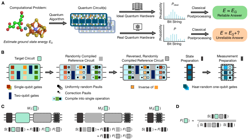
Figure 1: Establishing trust in quantum computations by estimating circuit execution fidelity. A. A quantum algorithm for gate-based quantum computers solves a computational problem by running one or more quantum circuits on a quantum computer, to sample from some probability distributions $P_{\textrm{ideal}}$. Real-world quantum computers implement circuits imperfectly, resulting in circuit outputs (bit strings) sampled from distributions $P$ that differ from $P_{\textrm{ideal}}$, causing inaccuracy in the algorithm’s solution. Quantifying the solution inaccuracy caused by these imperfections is difficult, because, for example, computing $P_{\textrm{ideal}}$ is generally infeasible using even the most powerful supercomputers. B. Our technique estimates the fidelity $F(c)$ with which an as-built quantum computer can execute some target circuit $c$ (green box), using motion reversal circuits built from the five reference (sub)circuits shown here. C. The three motion reversal circuits we use to estimate fidelity, $M_{i}(c)$, selectively use randomized compilation to isolate $F(c)$ without requiring that $c$ is randomly compiled. These motion reversal circuits are designed so that their mean adjusted success probabilities $S(\cdot)$ [see Eq. (8)] are approximately equal to the product of the fidelities of their constituent subcircuits. This means that the simple function of their mean adjusted success probabilities shown in D can be used to estimate $F(c)$.

Existing techniques for verifying the output of quantum computers Ferracin et al. (2021, 2019); Bennink (2021); Flammia and Liu (2011); Pallister et al. (2018); Mahadev (2018); Gheorghiu et al. (2019, 2019); Zhu et al. (2021); Barz et al. (2013) have complementary properties to ours. These methods can be divided into those that, like ours, quantify the accuracy with which a quantum circuit can be executed on a quantum computer that is noisy and error-prone but otherwise trusted, and methods for verifying the correct operation of a potentially malicious quantum computing server. Unlike our technique, the existing methods for quantifying the accuracy of circuit executions are either designed for special kinds of circuits—such as randomly compiled circuits Ferracin et al. (2021, 2019), circuits that create anti-concentrated states Bennink (2021), or Clifford circuits Pallister et al. (2018)—or are only efficient for special kinds of circuits Flammia and Liu (2011); Leone et al. (2022). In particular, direct fidelity estimation Flammia and Liu (2011) is a technique for measuring the execution fidelity of any circuit, but it is only efficient for circuits that can be efficiently simulated classically Leone et al. (2022). The existing techniques for verifying the output of a potentially malicious quantum computer—using interactive proofs, blind quantum computing, and cryptographic methods—require resource-intensive implementations of algorithms that are experimentally challenging Barz et al. (2013); Mahadev (2018); Gheorghiu et al. (2019, 2019); Zhu et al. (2021); Stricker et al. (2022). It is unlikely that they can be used to establish trust in the first practically important quantum computations.

Quantum circuits—An $n$-qubit quantum circuit $c$ is a sequence of $d$ layers of logic gates $l_{1}$, $l_{2}$, $\dots$, $l_{d}$, denoted by $c=l_{d}l_{d-1}\cdots l_{2}l_{1}$, where a layer $l$ consists of gates applied to disjoint sets of the $n$ qubits (see example in Fig. 1A). In this work, a circuit or layer $l$ ideally implements an $n$-qubit unitary $U(l)\in\mathbb{SU}(2^{n})$. Running a circuit $c$ consists of applying a state preparation that ideally initializes each of $n$ qubits in ${\left|0\right\rangle}$, then applying the layers of $c$ in turn, and then applying a measurement that ideally projects onto the computational basis. Our method assumes the ability to implement arbitrary single-qubit gates and an entangling two-qubit gate that is Clifford and self-inverse, e.g., CNOT. Note, however, that our technique can be applied to a circuit $c$ containing any gates, as we only require gates of this form in reference circuits against which $c$ is compared. We use $l_{\textrm{rev}}$ to denote the unique layer in which each gate in $l$ is replaced with its inverse, and $c_{\textrm{rev}}=l_{\textrm{rev},1}l_{\textrm{rev},2}\cdots l_{\textrm{rev},d}$ the motion reversal circuit, so $U(c_{\textrm{rev}})=U^{\dagger}(c)$ and $U(c_{\textrm{rev}}c)=\mathbb{I}$. The circuits used in our method will contain random layers and sub-circuits. A circuit containing random layers or subcircuits is a circuit-valued random variable, and is denoted using upper-case font and referred to as a randomized circuit. The expectation value, which is taken over all random variables within its argument, is denoted by $\mathbb{E}\{\cdot\}$.

Quantifying quantum computation accuracy—There are many ways to quantify how well a quantum computer can run some $n$-qubit circuit $c$. Each run of $c$ generates an $n$-bit string sampled from some probability distribution $P$ over $\{0,1\}^{n}$. In the presence of errors, this is typically different from the distribution from which $c$ is supposed to sample ($P_{\textrm{ideal}}$), given by

$$P_{\textrm{ideal},x}(c)={\left\langle x\right|}\;U(c){\left|0\right\rangle}^{\otimes n},$$ (1)

for $x\in\{0,1\}^{n}$. One way to quantify how accurately a quantum computer can implement $c$ is by some measure of the distance between $P$ and $P_{\textrm{ideal}}$ (see Fig. 1A). However, this typically requires knowing $P_{\textrm{ideal}}$, and using a classical computer to calculate or sample from $P_{\textrm{ideal}}$ is infeasible for most circuits with $n\gg 1$, including all computationally useful circuits.

An alternative way to quantify how accurately $c$ is implemented is by some notion of evolution accuracy, i.e., the difference between the implemented evolution $\phi(c)$ and the ideal unitary $U(c)$. This is a strictly more rigorous test of a quantum computer’s implementation of $c$, as phase errors are unobserved by a computational basis measurement. Testing evolution accuracy rather than comparing $P$ to $P_{\textrm{ideal}}$ is therefore important if $c$ is a subroutine, meaning that it is to be embedded within a variety of larger circuits. This is the case if $c$ prepares a state on which multiple non-commuting observables are to be measured, or if it is a multi-purpose computational primitive used within larger algorithms. To define notions of the evolution accuracy we require a mathematical model for $\phi(c)$. We use the standard “Markovian” model Nielsen et al. (2021) in which $\phi(c)$ is a superoperator that maps $n$-qubit quantum states to $n$-qubit quantum states. We compare this to the superoperator representation of the ideal evolution $U(c)$, denoted by $\mathcal{U}(c)$ and defined by $\mathcal{U}(c)[\rho]=U(c)\rho U^{\dagger}(c)$.

In this work we focus on estimating the entanglement fidelity of $\phi(c)$ to $\mathcal{U}(c)$, defined by

$$F(c)\equiv F(\mathcal{E}(c))=\langle\varphi|(\mathbb{I}\otimes\mathcal{E}(c))[|\varphi\rangle\langle\varphi|]|\varphi\rangle,$$ (2)

where $\mathcal{E}(c)=\mathcal{U}^{\dagger}(c)\phi(c)$ is $c$’s error map and $\varphi$ is any maximally entangled state of $2n$ qubits Nielsen (2002). This fidelity is linearly related to another widely-used fidelity variant—the average gate fidelity Nielsen (2002)

$$\bar{F}(c)\equiv\bar{F}(\mathcal{E}(c)) =\int d\psi\,{\left\langle\psi\right|}\mathcal{E}(c)[\psi]{\left|\psi\right\rangle},$$ (3)

$$={\left\langle\psi_{0}\right|}\mathbb{E}\{\mathcal{T}^{\dagger}\mathcal{E}(c)\mathcal{T}\}[\psi_{0}]{\left|\psi_{0}\right\rangle},$$ (4)

$$=\frac{2^{n}F(c)+1}{2^{n}+1}$$ (5)

where $d\psi$ is the Haar measure on pure states, $\psi_{0}$ is any pure state, and $\mathcal{T}$ is a superoperator-valued random variable with $\mathcal{T}[\rho]=T\rho T^{\dagger}$ where $T$ is a unitary 2-design over $\mathbb{SU}(2^{n})$ Magesan et al. (2012).

Fidelity estimation using motion reversal—Since the foundational work on fidelity estimation Emerson et al. (2007, 2005), motion reversal has been considered an intuitive but flawed basis for quantifying circuit execution accuracy. In this work, we show how a form of motion reversal circuits can be used for efficient and robust fidelity estimation. We therefore first explain why motion reversal is an appealing method for estimating fidelity and why, in its simplest form, it fails to do so reliably. The reverse of $c$ ($c_{\textrm{rev}}$) ideally implements $\mathcal{U}^{\dagger}(c)$. So, because $\phi(c)=\mathcal{U}(c)\mathcal{E}(c)$, we can isolate $c$’s error map if we follow $c$ by an ideal reverse evolution. By interrogating this error map with sufficiently diverse states and measurements, this motion reversal circuit can be used to estimate $F(c)$. Eq. (4) tells us that the states generated by a unitary 2-design are sufficiently diverse. In particular, consider the circuit $M(c)=T_{\textrm{rev}}c_{\textrm{rev}}cT$, where $T$ is a randomized circuit such that $U(T)$ is a unitary 2-design over $\mathbb{SU}(2^{n})$. Assume that all operations in $M(c)$ except $c$ are perfect, i.e., $\phi(c_{\textrm{rev}})=\mathcal{U}(c_{\textrm{rev}})$ etc. Then, by applying Eq. (4), we find that these circuits’ mean success probability $\bar{Q}=\mathbb{E}\{P_{0}(M(c))\}$ satisfies $\bar{Q}=\bar{F}(c)$ and is therefore related to $F(c)$ by

$$F(c)=(1+\nicefrac{{1}}{{2}}^{n})\bar{Q}-\nicefrac{{1}}{{2^{n}}}.$$ (6)

The problem with this fidelity estimation procedure is that no real quantum computer has access to perfect unitaries, state preparations, and measurements. Eq. (6) is not a reliable estimate of $F(c)$ because $\bar{Q}$ captures the impact of all errors in $M(c)=T_{\textrm{rev}}c_{\textrm{rev}}cT$, not just those in $c$. The error in $M(c)$ can be dominated by the error in the randomized state preparation and measurement subcircuits, $T$ and $T_{\textrm{rev}}$. This is because implementing a unitary 2-design requires a large circuit , and this makes fidelity estimation using a unitary 2-design infeasible on more than a few qubits Proctor et al. (2019, 2021b). Furthermore, counter-intuitive effects can occur, e.g., coherent errors in $c_{\textrm{rev}}$ can even exactly cancel coherent errors in $c$ Proctor et al. (2021a) yielding $\bar{Q}=1$ when $F(c)\ll 1$. This is a well-known issue with simple motion reversal. We solve these problems using a streamlined randomized state preparation and measurement procedure, and randomized motion reversal, which we now introduce in turn.

Streamlined fidelity estimation using local randomized states—We overcome the prohibitive size of the circuits required to implement an $n$-qubit unitary 2-design, by using local randomized state preparation and measurement of each of the $n$ qubits. Our insight is that an $n$-qubit unitary 2-design average can be mimicked using only single-qubit unitary 2-design averages, which require only single-qubit gates, and classical data processing. In particular, for any bit string $y$ and error map $\mathcal{E}$,

$$F(\mathcal{E})=\sum_{x}\left(-\nicefrac{{1}}{{2}}\right)^{h(x,y)}{\left\langle x\right|}\mathbb{E}\{\mathcal{L}^{\dagger}\mathcal{E}\mathcal{L}\}[{\left|y\right\rangle}{\left\langle y\right|}]{\left|x\right\rangle},$$ (7)

where $h(x,y)$ is the Hamming distance from $x$ to $y$, and $\mathcal{L}=\otimes_{i=1}^{n}\mathcal{L}_{i}$ where $\mathcal{L}_{i}[\rho]=L_{i}\rho L_{i}^{\dagger}$ and $L_{i}$ is a single-qubit unitary 2-design (see Appendix .1 for a proof). The summation over all bit strings, with the probability of each bit string multiplied by a Hamming distance dependent factor, accounts for the local nature of the randomized state preparation. This recovers the full power of an $n$-qubit unitary 2-design average using simple and efficient classical data processing. To use Eq. (7) to estimate fidelity from running motion reversal circuits we compute their adjusted success probability, defined by

$$S(c)=\sum_{k=0}^{n}\left(-\frac{1}{2}\right)^{k}h_{k}(c).$$ (8)

Here $h_{k}(c)$ is the probability that $c$ outputs a bit string $y$ whose Hamming distance from $c$’s target bit string $x_{c}$ is $k$, i.e., $h_{k}(c)=\sum_{y\in D_{k}}P_{y}(c)$ where $D_{k}=\{y\mid h(x_{c},y)=k\}$. A circuit’s target bit string $x_{c}$ is the bit string that satisfies $P_{\textrm{ideal},x_{c}}(c)=1$. Not all circuits have a target bit string, but all our motion reversal circuits do.

Equation (7) implies that we can estimate fidelity using a motion reversal circuit that does not include full $n$-qubit unitary 2-design averaging, and its prohibitive overhead. Instead of using the motion reversal circuit $M(c)=T_{\textrm{rev}}c_{\textrm{rev}}cT$, we can estimate $F(c)$ by executing instances of

$$M^{\prime}(c)=L_{\textrm{rev}}c_{\textrm{rev}}cL,$$ (9)

where $L$ is a randomized circuit such that $\mathcal{U}(L)=\mathcal{L}$ for $\mathcal{L}$ as stated above. We then estimate $\bar{S}=\mathbb{E}\{S(M^{\prime}(c))\}$. If all operations in $M^{\prime}(c)$ except $c$ are perfect, Eq. (7) implies that $F[\mathcal{E}(c)]=\bar{S}$. Although no operations can be implemented perfectly in practice, in streamlining our motion reversal circuit from $M(c)$ to $M^{\prime}(c)$ we have constructed a circuit where the error in the randomized state preparation and measurement circuits will not dominate the error in $c$ in the $n\gg 1$ regime, for interesting $c$. To construct a reliable fidelity estimation method, we now only require a method for distinguishing errors in $c$ from those in other parts of our motion reversal circuits.

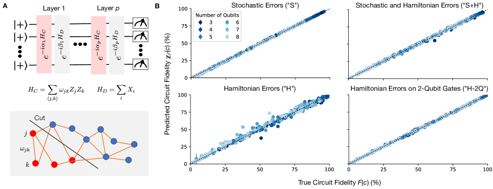
Figure 2: Applying our protocol to QAOA circuits using simulated data. A. Parameterized QAOA circuits for approximately solving the MaxCut problem on a weighted $n$-vertex graph consist of alternating applications of unitaries generated by two Hamiltonians: $H_{C}$, which encodes the graph, and $H_{D}$, which is a driver Hamiltonian that does not commute with $H_{C}$ Farhi et al. (2014). These unitaries are compiled into single-qubit gates and CNOTs. We randomly selected 300 distinct QAOA circuits, on up to $n=8$ qubits and with up to $p=10$ algorithmic layers. We applied our protocol to each circuit, with simulated data from four different families of error models. The variational parameters were randomly assigned for each circuit. B. Each circuit’s true process fidelity [$F(c)$], under the selected error model, versus the process fidelity predicted by our protocol [$\hat{\chi}_{F}(c)$], calculated by sampling 1000 mirror circuits of each type (see Fig. 1C) and simulating them under that error model. The four error models consist of stochastic Pauli errors on all gates, stochastic Pauli errors and Hamiltonian errors on all gates, Hamiltonian errors on all gates, and Hamiltonian errors on only two-qubit gates. The rates of the errors in each error model are randomly sampled for each QAOA circuit $c$. Each $\hat{\chi}_{F}(c)$ is shown with error bars (1 standard deviation, calculated using a nonparametetric boostrap) that, in most cases, are smaller than the data points.

Randomized motion reversal—Our aim is to robustly estimate $F(c)$, the fidelity of $c$’s overall error map $\mathcal{E}(c)$. Errors on the individual gates and layers of $c$ may coherently add or cancel, and this is fine—we wish to quantify how they impact the fidelity with which $c$ is implemented. However, fidelity estimation requires embedding $c$ within larger circuits. Now $c$’s errors could coherently add or cancel with errors in other parts of these larger circuits, e.g., $c_{\textrm{rev}}$. We need to prevent coherent addition or cancellation of errors between $c$ and other subcircuits without changing error propagation processes within $c$. To achieve this, we use selective randomized compilation Wallman and Emerson (2016); Knill (2005). A randomly compiled circuit has only stochastic errors, which cannot coherently add. In particular, we will compare $c$ to a randomly compiled motion reversal circuit. Unlike techniques designed to predict the fidelity of randomly compiled circuits Ferracin et al. (2021, 2019); Flammia (2021); Harper et al. (2020); Flammia and Wallman (2020); Erhard et al. (2019), our technique runs $c$ without randomized compilation. It uses randomly compiled circuits only to provide a stable reference frame against which $c$ can be compared.

Randomized compilation is defined on circuits with a particular structure, but we do not require $c$ to have that structure. So to implement randomized compilation on a circuit $c$, we first construct a circuit

$$\tilde{c}=l_{\tilde{d}}e_{\tilde{d}-1}l_{\tilde{d}-1}\cdots e_{2}l_{2}e_{1}l_{1},$$ (10)

that is logically equivalent to $c$, meaning that $\mathcal{U}(\tilde{c})=\mathcal{U}(c)$, where each $e_{i}$ layer contains only two-qubit gates that are Clifford and self-inverse, and each $l_{i}$ layer contains only single-qubit gates. Layers are allowed to be empty. Constructing a circuit of this form is always possible, as the set of all single-qubit gates along with any entangling gate forms a universal gate set Brylinski and Chen (2002). Note that $c$ may already have this form, in which case we can set $\tilde{c}=c$. This is the case in our simulations (reported below) and in the schematic of our method in Fig. 1B.

For a circuit $\tilde{c}$ with the form of Eq. (10), a randomized compilation of $\tilde{c}$, labeled $f_{\textrm{rc}}(\tilde{c})$, is constructed by first sampling $\tilde{d}$ $n$-qubit Pauli superoperators, $\mathcal{P}_{i}$ for $i=1,2,\dots,\tilde{d}$. We then replace each layer $l_{i}$ in $\tilde{c}$ with a new layer $l^{\prime}_{i}$ satisfying $\mathcal{U}(l^{\prime}_{i})=\mathcal{P}_{i}\mathcal{U}(l_{i})\mathcal{U}(e_{i-1})\mathcal{P}_{i-1}\mathcal{U}(e_{i-1})^{\dagger}$, with $\mathcal{P}_{0}$ defined to be the identity operator and $e_{0}$ an empty layer. This new circuit implements the same unitary as $\tilde{c}$ up to post-multiplication by a Pauli operator $\mathcal{P}_{\tilde{d}}$. In our context, $\mathcal{P}_{\tilde{d}}$ simply changes the circuit’s target bit string.

Robust mirror circuit fidelity estimation—Our MCFE protocol combines motion reversal with randomized compilation and streamlined, local randomized state preparation to robustly estimate $F(c)$. We use the three randomized circuits

$$M_{1}(c) =f_{\textrm{rc}}(L_{\textrm{rev}}\tilde{c}_{\textrm{rev}})cL,$$ (11)

$$M_{2}(c) =f_{\textrm{rc}}(L_{\textrm{rev}}\tilde{c}_{\textrm{rev}}\tilde{c}L),$$ (12)

$$M_{3}(c) =f_{\textrm{rc}}(L_{\textrm{rev}}L),$$ (13)

shown in Fig. 1B, which are based on the motion-reversal circuit of Eq. (9). Errors within the randomly compiled components of these circuits become purely stochastic after averaging. This enables separating out the errors due to the different subcircuits within $M_{i}(c)$, as the overall fidelity of a sequence of stochastic error channels is the product of their fidelities, to first order in their infidelities (See Appendix .3). Moreover, the fidelity of any error channel—such as $\mathcal{E}(c)$—followed by a stochastic error channel is equal to the product of the fidelities of these two channels, to first order in their infidelities (See Appendix .3). This means that $S_{i}\equiv S(\mathbb{E}\{M_{i}(c)\})$ is approximately the product of the fidelities of $M_{i}(c)$’s constituent subcircuits. In particular,

$$S_{1} \approx F_{0}F(\tilde{c}_{\textrm{rev}})F(c),$$ (14)

$$S_{2} \approx F_{0}F(\tilde{c}_{\textrm{rev}})F(\tilde{c}),$$ (15)

$$S_{3} \approx F_{0},$$ (16)

where $F_{0}$ is the fidelity of randomized state preparation and measurement operations (including contributions from errors in $L$ and $L_{\textrm{rev}}$, errors in the readout, and errors in preparing the standard input state). Furthermore, we have that

$$F(\tilde{c}_{\textrm{rev}})\approx F(\tilde{c})$$ (17)

as both circuits are randomly compiled and contain identical two-qubit gate layers. Therefore, as shown diagrammatically in Fig. 1C, we can combine the four approximate equalities of Eqs. (14)-(17) to compute $F(c)$:

$$F(c)\approx\frac{S_{1}}{\sqrt{S_{2}S_{3}}}.$$ (18)

This formula is approximate, and it can be improved upon by using polarization rather than fidelity. In particular, we approximate $F(c)$ by

$$\chi_{F}(c)=1-\frac{4^{n}-1}{4^{n}}\left(1-\frac{\mathbb{E}\{\gamma(M_{1}(c))\}}{\sqrt{\mathbb{E}\{\gamma(M_{2}(c))\}\mathbb{E}\{\gamma(M_{3}(c))\}}}\right),$$ (19)

where $\gamma(c)$ is a circuit’s effective polarization Proctor et al. (2021b)

$$\gamma(c)=\frac{4^{n}}{4^{n}-1}S(c)-\frac{1}{4^{n}-1}.$$ (20)

The difference between $\chi_{F}(c)$ and the simpler expression of Eq. (18) is negligible when $n\gg 1$, as $\chi_{F}(c)=\nicefrac{{S_{1}}}{{\sqrt{S_{2}S_{3}}}}+\mathcal{O}(\nicefrac{{1}}{{4^{n}}})$. Furthermore, note that $\chi_{F}(c)=F(c)$ exactly if (1) the error maps on $\tilde{c}_{\textrm{rev}}$ and $\tilde{c}$ are equal and (2) both these error maps and the state preparation and measurement error can be modelled by an $n$-qubit depolarizing channel. See Appendix .3 for further theoretical justification of our claim that $\chi_{F}(c)\approx F(c)$.

Our formula for $\chi_{F}(c)$ includes expectation values over large circuit ensembles, and we must estimate $\chi_{F}(c)$ from a finite amount of data. To do so, we sample $N_{i}\gg 1$ circuits from $M_{i}(c)$ for $i=1,2,3$. We run each one $K\geq 1$ times, and estimate each expectation value in Eq. (19) as the sample mean. This estimation can be done efficiently, because the required total number of samples $K_{\textrm{total}}=(N_{1}+N_{2}+N_{3})K$ to estimate $\chi_{F}(c)$ to a specified relative precision does not grow with $n$. In Appendix .2, we show that

$$N_{i}=\mathcal{O}\left(\frac{\ln(1/\delta)}{\alpha^{2}\gamma_{0}^{2}}\right)$$ (21)

circuits are sufficient to estimate $\chi_{F}(c)$ to relative precision $2\alpha$, with probability greater than $(1-\delta)^{3}$, when the average effective polarizations $\mathbb{E}\{\gamma(M_{i}(c))\}$ are bounded below by $\gamma_{0}$. Our protocol can therefore be efficiently applied in the $n\gg 1$ regime where direct verification of a quantum computation’s accuracy, via classical simulations, is intractable.

Simulations—We tested our method in simulations, by applying it to circuits that implement QAOA for the MaxCut problem on $n$-vertex weighted graphs Farhi et al. (2014). QAOA approximately solves MaxCut using the parameterized circuit shown in Fig. 2A, which is parameterized by the problem graph, the number of algorithmic layers $p$, and two length $p$ vectors of angles $\vec{\alpha},\vec{\beta}\in(-\pi,\pi]^{p}$. We applied our method to 300 distinct QAOA circuits, obtained by varying $n$ and $p$ ($n=3,4,\dots,8$ and $p=1,2,5,8,10$), and at each pair $(n,p)$ sampling 10 distinct $n$-vertex weighted graphs and random angle vectors $\vec{\alpha},\vec{\beta}$. For each QAOA circuit $c$, we sample $N$ of each of the three types of mirror circuit, and we simulate all $3N+1$ circuits under each of four different error models (detailed below). The main purpose of these simulations is to compare $\chi_{F}(c)$ to $F(c)$—as we do not expect $\chi_{F}(c)$ to exactly equal $F(c)$—rather than to study the impact of finite $N$ and $K$ on our estimate’s statistical uncertainty. We therefore sample many mirror circuits ($N=1000$) and compute the exact $\gamma$ for each circuit (equivalent to $K\to\infty$), as then finite-sample fluctuations will be small, i.e., $|\hat{\chi}_{F}(c)-\chi_{F}(c)|\ll 1$, and they will not obscure any discrepancies between $\chi_{F}(c)$ and $F(c)$.

Figure 2B shows $F(c)$ versus $\hat{\chi}_{F}(c)$ for all 300 QAOA circuits, with each of the scatter plots showing results for a different family of error models. These error models consist of stochastic Pauli errors on all gates (“S”), stochastic Pauli errors and Hamiltonian (i.e., coherent) errors on all gates (“S+H”), Hamiltonian errors on all gates (“H”), and Hamiltonian errors on only two-qubit gates (“H-2Q”) Blume-Kohout et al. (2021). The rates of the errors in each error model are randomly sampled for each QAOA circuit $c$, so each data point in Fig. 2B compares $\chi_{F}(c)$ and $F(c)$ for a unique QAOA circuit $c$ simulated under a unique error model. See Appendix .4 for details of these error models and simulations.

We find that $\chi_{F}(c)$ is a very good approximation to $F(c)$ under S, S+H, and H-2Q error models, whereas $\chi_{F}(c)$ differs from $F(c)$ more substantially for the H models. In all cases $\frac{1}{2}F(c)<\hat{\chi}_{F}(c)<2F(c)$ when $F(c)\geq 5\%$ [we do not expect low relative error for very small $F(c)$]. For S models the estimation error is particularly small, e.g., $|[\hat{\chi}_{F}(c)-F(c)]/F(c)|\leq 0.4\%$ for all circuits and S models in which $F(c)\geq 75\%$. The larger estimation error when there are Hamiltonian errors on both one- and two-qubit gates is consistent with our theory for our protocol—as applying our theory to these error models requires larger approximations. For example, general Hamiltonian errors on one-qubit gates introduces approximation into the theory of randomized compiling that we rely on to show that $\chi_{F}(c)\approx F(c)$. See Appendix .3 for further discussions.

Discussion—State-of-the-art quantum computers can no longer be simulated on classical supercomputers. This makes it impossible to directly quantify the accuracy of their output when running algorithms that do not have efficiently verifiable solutions. In this paper we have introduced an efficient and simple technique for estimating the fidelity with which a quantum circuit $c$ can be executed on a specific quantum computer. Our technique can be used to confirm that a full-scale quantum computation has been implemented with low error, even using hardware that suffers complex and not fully understood errors. Assessing the accuracy of a complex experiment and ascribing confidence in its output is a familiar challenge in experimental science, and our technique is a general solution to this problem for quantum computing systems.

The immediate use of our protocol is for quantifying the accuracy of NISQ computations. However, it will still be necessary to quantify circuit execution accuracy in the era of fault-tolerant quantum computation—because quantum computations on error corrected qubits will still suffer errors at the logical level, albeit at suppressed rates. We anticipate that the execution of our protocol at the logical level will enable efficient verification of future fault-tolerant quantum algorithmic circuits. Our method will therefore enable trustworthy quantum computation in both the NISQ computing era and beyond.

Supplemental Material

.1 Computing fidelity using local twirls

In this section we prove Eq. (7), where we claim that for any error map $\mathcal{E}$, $F(\mathcal{E})$ is equal to the quantity

$$\Upsilon\equiv\sum_{x}\left(-\nicefrac{{1}}{{2}}\right)^{h(x,y)}{\left\langle x\right|}\mathbb{E}\{\mathcal{L}^{\dagger}\mathcal{E}\mathcal{L}\}[{\left|y\right\rangle}{\left\langle y\right|}]{\left|x\right\rangle},$$ (22)

where $y$ is any $n$-bit string, $h(x,y)$ is the Hamming distance from $x$ to $y$, and

$$\mathcal{L}=\otimes_{i=1}^{n}\mathcal{L}_{i}.$$ (23)

Here $\mathcal{L}_{i}[\rho]=L_{i}\rho L_{i}^{\dagger}$ and $L_{i}$ is a single-qubit unitary 2-design. It is useful to first rewrite $\Upsilon$ as

$$\Upsilon=\sum_{k=0}^{n}\left(-\nicefrac{{1}}{{2}}\right)^{k}h_{k}(\mathcal{E}),$$ (24)

where

$$h_{k}(\mathcal{E})=\sum_{h(x,y)=k}{\left\langle x\right|}\mathbb{E}\{\mathcal{L}^{\dagger}\mathcal{E}\mathcal{L}\}[{\left|y\right\rangle}{\left\langle y\right|}]{\left|x\right\rangle},$$ (25)

is the probability of observing any bit string $x$ that is a Hamming distance of $k$ from $y$.

We begin by noting that twirling $\mathcal{E}$ by a tensor product of single-qubit 2-design projects $\mathcal{E}$ onto the $2^{n}$ dimensional space spanned by tensor products of single-qubit depolarizing channels Gambetta et al. (2012). That is

$$\bar{\mathcal{E}}=\mathbb{E}\{\mathcal{L}^{\dagger}\mathcal{E}\mathcal{L}\}$$ (26)

is a stochastic Pauli channel with (1) equal marginal probabilities to induce an $X$, $Y$ or $Z$ error on any fixed qubit, and (2) a fidelity equal to that of $\mathcal{E}$, i.e.,

$$F(\bar{\mathcal{E}})=F(\mathcal{E}).$$ (27)

Therefore, in the following we prove that $\Upsilon=F(\bar{\mathcal{E}})$, from which Eq. (7) follows immediately.

The channel $\bar{\mathcal{E}}$ is entirely described by a set of $2^{n}$ probabilities $\{r_{Q}(\bar{\mathcal{E}})\}$ where $Q$ runs over all possible subsets of the $n$ qubits and $r_{Q}(\bar{\mathcal{E}})$ is the probability that $\bar{\mathcal{E}}$ applies a nontrivial Pauli error to those qubits—meaning that $\bar{\mathcal{E}}$ applies a Pauli that is not the identity on each qubit in $Q$ and that is the identity on all other qubits. Conditioned on $\bar{\mathcal{E}}$ applying an error to the qubit set $Q$, the error that occurs is a uniformly random sample from the set of $3^{W(Q)}$ possible $n$-qubit Pauli operators that are the identity on all but the qubits in $Q$, where $W(Q)$ denotes the size of the set $Q$. Therefore, if an error occurs on the qubit set $Q$, which is a weight $w=W(Q)$ error, its action on a computational basis state ${\left|y\right\rangle}{\left\langle y\right|}$ is to flip $k$ of the bits with probability

$$A_{kw}={w\choose k}\frac{2^{k}}{3^{w}},$$ (28)

when $k\leq w$ and $A_{kw}=0$ otherwise. This is because the number of bits flipped corresponds to the number of $X$ and $Y$ errors in the applied Pauli error, and $A_{kw}$ is the probability that a uniformly random weight $w$ Pauli contains $(w-k)$ $Z$ operators.

The quantity $h_{k}(\mathcal{E})$ is equal to the total probability of $\bar{\mathcal{E}}$ causing $k$ bit flips on $y$. This can be computed by summing, over all qubit subsets $Q$, the probability $r_{Q}(\bar{\mathcal{E}})$ of an error occurring on qubit set $Q$ multiplied by the probability that an error on that subset causes $k$ bit flips, which is $A_{kW(Q)}$. That is

$$h_{k}(\mathcal{E}) =\sum_{Q}A_{kW(Q)}r_{Q}(\bar{\mathcal{E}}),$$ (29)

$$=\sum_{w}A_{kw}r_{w}(\bar{\mathcal{E}})$$ (30)

where $r_{w}(\bar{\mathcal{E}})=\sum_{Q\mid W(Q)=w}r_{Q}(\bar{\mathcal{E}})$ is the probability that $\bar{\mathcal{E}}$ applies any weight $w$ Pauli. This equation can be written as

$$\vec{h}(\mathcal{E})=A\vec{r}(\bar{\mathcal{E}}).$$ (31)

The fidelity of $\bar{\mathcal{E}}$ is the probability that it applies the identity Pauli, so $F(\bar{\mathcal{E}})=r_{0}(\bar{\mathcal{E}})$, and therefore,

$$F(\bar{\mathcal{E}})=[A^{-1}\vec{h}(\mathcal{E})]_{0}.$$ (32)

To obtain our result we therefore just need the first row of the inverse of $A$, which is given by

$$[A^{-1}]_{0k}=\left(-\nicefrac{{1}}{{2}}\right)^{k}.$$ (33)

Substituting this into Eq. (32) yields $F(\bar{\mathcal{E}})=\Upsilon$, implying $F(\mathcal{E})=\Upsilon$, by Eq. (27).

.2 Resource requirements

Our procedure approximates the fidelity $F(c)$ of a quantum circuit, $c$, by estimating the quantity $\chi_{F}(c)$, which is defined in Eq. (19). In this section, we derive Eq. (21), which defines the number of samples (experimental runs of quantum circuits) needed to guarantee that our estimate is accurate to a specified relative error, with high probability. For the purposes of this section, we assume each circuit is run only $K=1$ times.

For any given quantum circuit, $c$, we estimate $\chi_{F}(c)$ by first estimating the expected effective polarization

$$\gamma_{i}=\mathbb{E}\{\gamma(M_{i}(c))\}$$ (34)

for each of three ensembles of mirror circuits, $M_{i}(c)$ with $i=1,2,3$. For each ensemble $M_{i}(c)$, we draw $N$ random circuits, run each circuit $K=1$ times on the quantum computer, determine the Hamming distance ($\{h_{j}^{(i)}\}_{j=1}^{N}$) of each resulting bit string to the circuit’s target bit string, and compute the quantity:

$$\hat{\gamma}_{i}=\sum_{j=1}^{N}\frac{1}{N}\left(\frac{4^{n}}{4^{n}-1}\left(-\frac{1}{2}\right)^{h_{j}^{(i)}}-\;\frac{1}{4^{n}-1}\right)$$ (35)

The quantity $\hat{\gamma}_{i}$ is an unbiased estimate of the expected polarization, as its expected value $\mathbb{E}\{\hat{\gamma}_{i}\}$ is equal to the true (unknown) expected polarization $\gamma_{i}$. Because each circuit is run only once, $\hat{\gamma}_{i}$ is a sum of bounded, independent random variables, and so obeys Hoeffding’s concentration inequality Hoeffding (1963):

$$P\big{(}|\hat{\gamma}_{i}-\gamma_{i}|\geq\epsilon\big{)}\leq 2\exp\left(-\frac{8}{9}\left(\frac{4^{n}-1}{4^{n}}\right)^{2}\epsilon^{2}N\right).$$ (36)

If we are assured that the mean effective polarizations of each of the circuit ensembles $\gamma_{i}$ is greater than some minimum, $\gamma_{0}$, then we can replace the additive error in Eq. (36) with a relative error. For any $\alpha>0$:

$$P\big{(}\left|\hat{\gamma}_{i}-\gamma_{i}\right|\geq\alpha\,\gamma_{i}\big{)}\leq\delta$$ (37)

where

$$\delta=2\exp\left(-\frac{8}{9}\left(\frac{4^{n}-1}{4^{n}}\right)^{2}\alpha^{2}\gamma_{0}^{2}N\right).$$ (38)

The fidelity of circuit $c$ is estimated using Eq. (19), which we reproduce here written in terms of $\gamma_{i}$:

$$\chi_{F}(c)=1-\frac{4^{n}-1}{4^{n}}\left(1-\frac{\gamma_{1}}{\sqrt{\gamma_{2}\gamma_{3}}}\right),$$

Using the bound above for the relative error in our estimates $\hat{\gamma}_{i}$, we can bound the error in our estimate of $\chi_{F}(c)$. The estimate of $\chi_{F}(c)$ depends linearly in the estimate of the ratio $R(c)$, defined as:

$$\hat{R}(c)=\frac{\hat{\gamma}_{1}}{\sqrt{\hat{\gamma}_{2}\hat{\gamma}_{3}}}.$$ (39)

The true value of this ratio is given in terms of the expectation values of $\gamma(M_{i}(c))$.

$$R(c)=\frac{\gamma_{1}}{\sqrt{\gamma_{2}\gamma_{3}}}.$$ (40)

With probability greater than $(1-\delta)^{3}$, all three effective polarization estimates, $\hat{\gamma}_{i}$, will have relative error less than $\alpha$. Within this range, the worst case error on the estimate of $\hat{R}(c)$ occurs when $\hat{\gamma}_{1}$ has relative error $(1\pm\alpha)$ , and both $\hat{\gamma}_{2}$ and $\hat{\gamma}_{3}$ have relative errors $(1\mp\alpha)$.

$$R^{\pm}(c) =\frac{\gamma_{1}(1\pm\alpha)}{\sqrt{\gamma_{2}(1\mp\alpha)\gamma_{3}(1\mp\alpha)}}$$ (41)

$$=R(c)\frac{1\pm\alpha}{1\mp\alpha},$$ (42)

$$\simeq R(c)(1\pm 2\alpha).$$ (43)

In the limit of small $\alpha$, we then have

$$P\Big{(}|\hat{R}(c)-R(c)|\leq 2\alpha\;R(c)\Big{)}\geq(1-\delta)^{3}.$$ (44)

Similarly, our estimate $\hat{\chi}_{F}(c)$ satisfies:

$$P\Big{(}|\hat{\chi}_{F}(c)-\chi_{F}(c)|\leq 2\alpha\;\chi_{F}(c)\Big{)}\geq(1-\delta)^{3}.$$ (45)

For any fixed value of $\delta$, we can solve for $N$, the minimum number of circuits that must be sampled for each ensemble $M_{i}(c)$ to achieve this bound:

$$N\geq\frac{9}{8}\left(\frac{4^{n}}{4^{n}-1}\right)^{2}\frac{\ln(2/\delta)}{\alpha^{2}\gamma_{0}^{2}}.$$ (46)

This is weakly decreasing in the number of qubits $n$. We can remove the dependence on $n$ by taking the limit of a single qubit. In this case, we have:

$$N\geq\frac{2\ln(2/\delta)}{\alpha^{2}\gamma_{0}^{2}},$$ (47)

which implies Eq. (21) stated in the main text.

.3 Relating $\chi_{F}(c)$ to fidelity

In this section we provide additional theoretical justification for our claim that $\chi_{F}(c)\approx F(c)$. Our theory uses the polarization of an error map $\mathcal{E}$, which is defined by

$$\lambda(\mathcal{E})=\frac{4^{n}}{4^{n}-1}F(\mathcal{E})-\frac{1}{4^{n}-1}.$$ (48)

Note that $\lambda(\mathcal{E})=F(\mathcal{E})+\mathcal{O}(\nicefrac{{1}}{{4^{n}}})$, so the difference between polarization and fidelity is negligible for $n\gg 1$.

Our circuit ensembles, $M_{i}(c)$ with $i=1,2,3$, are designed so that

$$\gamma_{i}\equiv\mathbb{E}\{\gamma(M_{i}(c))\}$$ (49)

is approximately equal to the product of the polarizations of the constituent subcircuits in the $M_{i}(c)$ circuits. More precisely, we claim that

$$\gamma_{1} \approx\gamma_{0}\gamma_{\textrm{rev}}\lambda(c),$$ (50)

$$\gamma_{2} \approx\gamma_{0}\gamma_{\textrm{rev}}^{2},$$ (51)

$$\gamma_{3} \approx\gamma_{0},$$ (52)

where $\gamma_{0}$ is related to the mean polarization (or fidelity) of the randomized state preparation and measurement, $\gamma_{\textrm{rev}}$ is related to the mean polarization (or fidelity) of a random compilation of $\tilde{c}_{\textrm{rev}}$, and $\lambda(c)$ is the polarization of $\mathcal{E}(c)$. If these three equations approximately hold, then $\lambda(c)\approx\nicefrac{{\gamma_{1}}}{{\sqrt{\gamma_{2}\gamma_{3}}}}$ and therefore $\chi_{F}(c)\approx F(c)$. The aim of the remainder of this section is to provide theoretical justification for Eqs. (50)-(52). Note that in the main text we state that $S_{i}\equiv\mathbb{E}\{S(M_{i}(c))\}$ is approximately equal to the product of the fidelities of the constituent subcircuits, rather than that the effective polarizations are equal to the product of the polarizations of the constituent subcircuits. These claims are equivalent as $\gamma(c)=S(c)+\mathcal{O}(\nicefrac{{1}}{{4^{n}}})$ and $\lambda(\mathcal{E})=F(\mathcal{E})+\mathcal{O}(\nicefrac{{1}}{{4^{n}}})$, i.e., the approximations in Eqs. (50)-(52) imply the approximations stated in the main text up to $\mathcal{O}(\nicefrac{{1}}{{4^{n}}})$ corrections.

Throughout this section we use the standard “Markovian” model for errors in quantum computers Nielsen et al. (2021). Imperfect initialization into ${\left|0\right\rangle}{\left\langle 0\right|}^{\otimes n}$ is represented by an $n$-qubit state $\rho$. An imperfect measurement in the computational basis is represented by a positive-operator valued measure $\{E_{x}\}$, i.e., $E_{x}$ are positive operators satisfying $\sum_{x}E_{x}=\mathbb{I}$, where $E_{x}$ is a measurement effect corresponding to the result $x$. An imperfect implementation of a circuit $c=l_{d}\cdots l_{2}l_{1}$ is a completely positive and trace preserving superoperator $\phi(c)$. Moreover, $\phi(c)=\phi(l_{d})\cdots\phi(l_{2})\phi(l_{1})$, where $\phi(l_{i})$ are superoperators for the layers. The probability of observing $x$ when running circuit $c$ is then given by

$$P_{x}(c)=\textrm{Tr}\left\{E_{x}\phi(c)[\rho]\right\}.$$ (53)

.3.1 The state preparation and measurement ensemble

First we analyze the randomized state preparation and measurement mirror circuit ensemble, $M_{3}(c)$. For these circuits

$$P_{x}(M_{3}(c))=\textrm{Tr}\left\{E_{x}\phi(f_{\textrm{rc}}(L_{\textrm{rev}}L))[\rho]\right\}.$$ (54)

To derive a formula for $\gamma_{3}$ we make some simplifying assumptions about the operations within $M_{3}(c)$. We model all errors in $L$, $L_{\textrm{rev}}$, the state preparation, and the readout, by an $L$-independent stochastic Pauli channel $\mathcal{E}_{\textrm{spam}}$ preceding $L_{\textrm{rev}}$. Under this assumption

$$P_{x}(M_{3}(c)) ={\left\langle x\right|}\mathcal{L}^{\dagger}\mathcal{E}_{\textrm{spam}}\mathcal{L}\mathcal{P}[{\left|0\right\rangle}{\left\langle 0\right|}]{\left|x\right\rangle}$$ (55)

$$={\left\langle x\right|}\mathcal{L}^{\dagger}\mathcal{E}_{\textrm{spam}}\mathcal{L}[{\left|y\right\rangle}{\left\langle y\right|}]{\left|x\right\rangle},$$ (56)

where $\mathcal{L}=\mathcal{U}(L)$, and $y$ is a uniformly random bit string. Therefore

$$S_{3} \equiv\mathbb{E}\{S(M_{3}(c))\},$$ (57)

$$=\mathbb{E}\left\{\sum_{k=0}^{n}\left(-\frac{1}{2}\right)^{k}\sum_{h(x,y)=k}{\left\langle x\right|}\mathcal{L}^{\dagger}\mathcal{E}_{\textrm{spam}}\mathcal{L}[{\left|y\right\rangle}{\left\langle y\right|}]{\left|x\right\rangle}\right\},$$ (58)

$$=\mathbb{E}_{y}\left\{\sum_{x}\left(-\frac{1}{2}\right)^{h(x,y)}\mathbb{E}_{\mathcal{L}}({\left\langle x\right|}\mathcal{L}^{\dagger}\mathcal{E}_{\textrm{spam}}\mathcal{L}[{\left|y\right\rangle}{\left\langle y\right|}]{\left|x\right\rangle})\right\},$$ (59)

$$=F(\mathcal{E}_{\textrm{spam}}),$$ (60)

where the first equality holds by definition, and the second equality is obtained by substituting Eq. (56) into the definition of $S(\cdot)$ in Eq. (8) [note that here $\sum_{h(x,y)=k}$ denotes summation over all bit strings $x$ and $y$ such that $h(x,y)=k$]. The third equality holds by the linearity of the expectation value, and the fourth equality holds from Eq. (7) (which holds for any value of $y$, and so it holds when averaging over all values of $y$). By subtracting 1 from each side of $S_{3}=F(\mathcal{E}_{\textrm{spam}})$ and then multiplying both sides by $\nicefrac{{4^{n}}}{{4^{n}-1}}$, using Eqs. (20) and (48) we obtain

$$\gamma_{3}=\lambda(\mathcal{E}_{\textrm{spam}}).$$ (61)

This is Eq. (52) with $\gamma_{0}=\lambda(\mathcal{E}_{\textrm{spam}})$.

.3.2 Randomized compilation

Deriving Eqs. (50) and (51) relies on the theory of randomized compilation Wallman and Emerson (2016). Randomized compilation is a key ingredient in our method, because it converts general errors into stochastic Pauli channels. Consider any circuit $\tilde{c}$ of the form of Eq. (10), i.e., $\tilde{c}=l_{\tilde{d}}e_{\tilde{d}-1}l_{\tilde{d}-1}\cdots e_{1}l_{1}$. For simplicity we will assume that errors in layers of one-qubit gates (the $l_{i}$ layers) are dominated by errors in layers of two-qubit gates (the $e_{i}$ layers), so that we can approximate $\phi(l_{i})$ by $\mathcal{U}(l_{i})$. No additional approximations are required to extended the following theory to the case in which single-qubit gate layers are subject to stochastic Pauli errors, with error rates that may be comparable or larger than those on the two-qubit gates, in the case where these Pauli error channels are independent of the random Pauli that is compiled into the layer .

Under the assumption that $\phi(l_{i})=\mathcal{U}(l_{i})$ for any single-qubit layer $l_{i}$, and defining $\mathcal{E}(e_{i})$ by $\phi(e_{i})=\mathcal{U}(e_{i})\mathcal{E}(e_{i})$, we have that

$$\phi(f_{\textrm{rc}}(\tilde{c}))=\cdots\mathcal{U}(e_{2})\mathcal{E}(e_{2})\mathcal{P}_{2}\mathcal{U}(l_{2})\mathcal{P}^{*}_{1}\mathcal{U}(e_{1})\mathcal{E}(e_{1})\mathcal{P}_{1}\mathcal{U}(l_{1}),$$ (62)

where the $\mathcal{P}_{i}$ are random Pauli operators and $\mathcal{P}_{i}^{*}=\mathcal{U}(e_{i})\mathcal{P}_{i}\mathcal{U}(e_{i})^{\dagger}$.

Averaging over the Pauli operators results in Pauli twirling of the error channels for the two-qubit gate layers. In particular, the mean of $\phi(f_{\textrm{rc}}(\tilde{c}))$ over all but the final random Pauli operator, i.e., the superoperator

$$\bar{\phi}(f_{\textrm{rc}}(\tilde{c}))=\mathbb{E}_{\mathcal{P}_{i},i<d}\{\phi(f_{\textrm{rc}}(\tilde{c}))\},$$ (63)

is given by Wallman and Emerson (2016)

$$\bar{\phi}(f_{\textrm{rc}}(\tilde{c}))=\mathcal{P}_{\tilde{d}}\mathcal{U}(l_{\tilde{d}})\prod_{k=1}^{\tilde{d}-1}\mathcal{U}(e_{k})\mathcal{S}(e_{k})\mathcal{U}(l_{k}),$$ (64)

where $\mathcal{S}(e_{k})$ is a stochastic Pauli channel given by

$$\mathcal{S}(e_{k})=\mathbb{E}_{\mathcal{P}}\{\mathcal{P}\mathcal{E}(e_{k})\mathcal{P}\}.$$ (65)

.3.3 The $M_{1}(c)$ ensemble

We now consider the $M_{1}(c)$ circuit ensemble, and derive the approximate equality $\gamma_{1}\approx\gamma_{0}\gamma(\tilde{c}_{\textrm{rev}})\gamma(c)$, where

$$\tilde{c}_{\textrm{rev}}=l_{1,\textrm{rev}}e_{1}\dots l_{\tilde{d}-1,\textrm{rev}}e_{\tilde{d}-1}l_{\tilde{d},\textrm{rev}}.$$ (66)

Consider the superoperator $\phi(f_{\textrm{rc}}(\tilde{c}_{\textrm{rev}})c)$ which can be decomposed as

$$\phi(f_{\textrm{rc}}(\tilde{c}_{\textrm{rev}})c)=\phi(f_{\textrm{rc}}(\tilde{c}_{\textrm{rev}}))\mathcal{U}(c)\mathcal{E}(c).$$ (67)

We now apply the theory of randomized compilation, and the model for the state preparation and measurement error, introduced above, to derive a formula for the action of $M_{1}(c)$ averaged over randomized compilations. The superoperator for $M_{1}(c)$ obtained when averaging over all Pauli operators in the randomized compilation of $\tilde{c}_{\textrm{rev}}$ except the last Pauli operator, is given by

$$\bar{\phi}(M_{1}(c)) =\mathcal{P}\mathcal{L}^{\dagger}\mathcal{E}_{\textrm{spam}}\bar{\mathcal{E}}(\tilde{c}_{\textrm{rev}})\mathcal{U}^{\dagger}(c)\mathcal{U}(c)\mathcal{E}(c)\mathcal{L},$$ (68)

where $\mathcal{P}$ is a random Pauli, and

$$\bar{\mathcal{E}}(\tilde{c}_{\textrm{rev}})=\mathcal{U}_{1}\mathcal{S}_{1}\mathcal{U}_{1}^{\dagger}\cdots\,\mathcal{U}_{\tilde{d}-1}\mathcal{S}_{\tilde{d}-1}\mathcal{U}_{\tilde{d}-1}^{\dagger},$$ (69)

with $\mathcal{S}_{i}=\mathcal{S}(e_{i})$, and $\mathcal{U}_{i}=\mathcal{U}(l_{1,\textrm{rev}}e_{1}l_{2,\textrm{rev}}\cdots e_{i})$. By defining $\tilde{\mathcal{L}}=\mathcal{L}\mathcal{P}$ (which is identically distributed to $\mathcal{L}$), we then have that

$$\bar{\phi}(M_{1}(c)) =\tilde{\mathcal{L}}^{\dagger}\mathcal{E}_{\textrm{spam}}\bar{\mathcal{E}}(\tilde{c}_{\textrm{rev}})\mathcal{E}(c)\tilde{\mathcal{L}}\mathcal{P}.$$ (70)

We therefore have that

$$P_{x}[M_{1}(c)] ={\left\langle x\right|}\tilde{\mathcal{L}}^{\dagger}\mathcal{E}_{\textrm{spam}}\bar{\mathcal{E}}(\tilde{c}_{\textrm{rev}})\mathcal{E}(c)\tilde{\mathcal{L}}\mathcal{P}[{\left|0\right\rangle}{\left\langle 0\right|}]{\left|x\right\rangle},$$ (71)

$$={\left\langle x\right|}\tilde{\mathcal{L}}^{\dagger}\mathcal{E}_{\textrm{spam}}\bar{\mathcal{E}}(\tilde{c}_{\textrm{rev}})\mathcal{E}(c)\tilde{\mathcal{L}}[{\left|y\right\rangle}{\left\langle y\right|}]{\left|x\right\rangle},$$ (72)

where $y$ is a uniformly random bit string. This equation has the same form as Eq. (56), with $\mathcal{E}_{\textrm{spam}}\to\mathcal{E}_{\textrm{spam}}\bar{\mathcal{E}}(c_{\textrm{rev}})\mathcal{E}(c)$. Therefore, we can apply Eqs. (56)-(61) to obtain

$$\gamma_{1}=\lambda\left(\mathcal{E}_{\textrm{spam}}\bar{\mathcal{E}}(\tilde{c}_{\textrm{rev}})\mathcal{E}(c)\right).$$ (73)

To obtain Eq. (50) we use the approximation

$$\lambda\left(\mathcal{E}_{\textrm{spam}}\bar{\mathcal{E}}(\tilde{c}_{\textrm{rev}})\mathcal{E}(c)\right) \approx\lambda\left(\mathcal{E}_{\textrm{spam}}\right)\lambda\left(\bar{\mathcal{E}}(\tilde{c}_{\textrm{rev}})\right)\lambda\left(\mathcal{E}(c)\right),$$ (74)

$$=\gamma_{0}\gamma_{\textrm{rev}}\lambda\left(c\right)$$ (75)

where to obtain the latter equality we defined

$$\gamma_{\textrm{rev}}=\lambda(\bar{\mathcal{E}}(\tilde{c}_{\textrm{rev}}))$$ (76)

Before we justify the approximation used in Eq. (74), we turn to $M_{2}(c)$.

.3.4 The $M_{2}(c)$ ensemble

We now consider the $M_{2}(c)$ circuit ensemble, and derive the approximate equality $\gamma_{2}\approx\gamma_{0}\gamma_{\textrm{rev}}^{2}$. As with $M_{1}(c)$, we use the theory of randomized compilation and our model for the state preparation and measurement error. This theory can be used to show that the mean superoperator for $M_{2}(c)$, obtained by averaging over all Pauli operators in the randomized compilation of $\tilde{c}_{\textrm{rev}}$ and $\tilde{c}$ except the last Pauli operator, is given by

$$\bar{\phi}(M_{2}(c)) =\mathcal{P}\mathcal{L}^{\dagger}\mathcal{E}_{\textrm{spam}}\bar{\mathcal{E}}(\tilde{c}_{\textrm{rev}})\mathcal{U}^{\dagger}(c)\mathcal{U}(c)\bar{\mathcal{E}}(\tilde{c})\mathcal{L},$$ (77)

$$=\tilde{\mathcal{L}}^{\dagger}\mathcal{E}_{\textrm{spam}}\bar{\mathcal{E}}(\tilde{c}_{\textrm{rev}})\bar{\mathcal{E}}(\tilde{c})\tilde{\mathcal{L}}\mathcal{P},$$ (78)

where $\bar{\mathcal{E}}(\tilde{c}_{\textrm{rev}})$ is defined in Eq. (69), and

$$\bar{\mathcal{E}}(\tilde{c})=\mathcal{V}_{\tilde{d}-1}^{\dagger}\mathcal{S}_{\tilde{d}-1}\mathcal{V}_{\tilde{d}-1}\cdots\mathcal{V}_{1}^{\dagger}\mathcal{S}_{1}\mathcal{V}_{1}$$ (79)

with $\mathcal{S}_{i}=\mathcal{S}(e_{i})$ and $\mathcal{V}_{i}=\mathcal{U}(l_{i}\cdots e_{1}l_{1})$. We therefore have that

$$P_{x}[M_{2}(c)] ={\left\langle x\right|}\tilde{\mathcal{L}}^{\dagger}\mathcal{E}_{\textrm{spam}}\bar{\mathcal{E}}(\tilde{c}_{\textrm{rev}})\bar{\mathcal{E}}(\tilde{c})\tilde{\mathcal{L}}\mathcal{P}[{\left|0\right\rangle}{\left\langle 0\right|}]{\left|x\right\rangle},$$ (80)

$$={\left\langle x\right|}\tilde{\mathcal{L}}^{\dagger}\mathcal{E}_{\textrm{spam}}\bar{\mathcal{E}}(\tilde{c}_{\textrm{rev}})\bar{\mathcal{E}}(\tilde{c})\tilde{\mathcal{L}}[{\left|y\right\rangle}{\left\langle y\right|}]{\left|x\right\rangle},$$ (81)

where $y$ is a uniformly random bit string. This equation has the same form as Eq. (56), with $\mathcal{E}_{\textrm{spam}}\to\mathcal{E}_{\textrm{spam}}\bar{\mathcal{E}}(\tilde{c}_{\textrm{rev}})\bar{\mathcal{E}}(\tilde{c})$. Therefore, we can apply Eqs. (56)-(61) to obtain

$$\gamma_{2}=\lambda\left(\mathcal{E}_{\textrm{spam}}\bar{\mathcal{E}}(\tilde{c}_{\textrm{rev}})\bar{\mathcal{E}}(\tilde{c})\right).$$ (82)

To obtain Eq. (51) we first use the approximation

$$\lambda\left(\mathcal{E}_{\textrm{spam}}\bar{\mathcal{E}}(\tilde{c}_{\textrm{rev}})\bar{\mathcal{E}}(\tilde{c})\right) \approx\lambda\left(\mathcal{E}_{\textrm{spam}}\right)\lambda\left(\bar{\mathcal{E}}(\tilde{c}_{\textrm{rev}})\right)\lambda\left(\bar{\mathcal{E}}(\tilde{c})\right).$$ (83)

We then substitute into this equation the approximation

$$\lambda(\bar{\mathcal{E}}(\tilde{c}_{\textrm{rev}}))\approx\lambda(\bar{\mathcal{E}}(\tilde{c})),$$ (84)

resulting in

$$\lambda\left(\mathcal{E}_{\textrm{spam}}\bar{\mathcal{E}}(\tilde{c}_{\textrm{rev}})\bar{\mathcal{E}}(\tilde{c})\right) \approx\lambda\left(\mathcal{E}_{\textrm{spam}}\right)\lambda\left(\bar{\mathcal{E}}(\tilde{c}_{\textrm{rev}})\right)^{2},$$ (85)

$$=\gamma_{0}\gamma_{\textrm{rev}}^{2},$$ (86)

which is Eq. (51).

The approximation of Eq. (83) is justified below, but first we address the approximation of Eq. (84). Using $\mathcal{U}_{i}^{\dagger}=e_{i}\mathcal{V}_{i}$, we have that

$$\mathcal{E}^{\dagger}(\tilde{c}_{\textrm{rev}}) =\mathcal{U}_{\tilde{d}-1}\mathcal{S}_{\tilde{d}-1}\mathcal{U}_{\tilde{d}-1}^{\dagger}\cdots\mathcal{U}_{1}\mathcal{S}_{1}\mathcal{U}_{1}^{\dagger},$$ (87)

$$=\mathcal{V}_{\tilde{d}-1}^{\dagger}\mathcal{S}^{\prime}_{\tilde{d}-1}\mathcal{V}_{\tilde{d}-1}\cdots\mathcal{V}_{1}^{\dagger}\mathcal{S}^{\prime}_{1}\mathcal{V}_{1},$$ (88)

where $\mathcal{S}^{\prime}_{i}=\mathcal{U}(e_{i})^{\dagger}\mathcal{S}_{i}\mathcal{U}(e_{i})$. If $\mathcal{S}^{\prime}_{i}=\mathcal{S}_{i}$ [which is true if $\mathcal{E}(e_{i})$ commutes with $\mathcal{U}(e_{i})$] then $\mathcal{E}^{\dagger}(\tilde{c}_{\textrm{rev}})=\mathcal{E}(\tilde{c})$, and so Eq. (84) holds exactly. More generally, conjugating the Pauli channel $\mathcal{S}_{i}$ by $\mathcal{U}(e_{i})$ simply permutes the error rates of $\mathcal{S}_{i}$ ($e_{i}$ contains only Clifford gates). This can have some impact on the rate that stochastic errors on different layers cancel—impacting the polarization of the composite error map and meaning that $\lambda(\bar{\mathcal{E}}(\tilde{c}_{\textrm{rev}}))$ does not exactly equal $\lambda(\bar{\mathcal{E}}(\tilde{c}))$—but typically this impact will be very small (see theory below), resulting in Eq. (84) holding approximately for the same reasons that Eqs. (74) and (85) approximately hold.

.3.5 Approximate formula for the polarization of composed channels

Our theory supporting the claim that $\chi_{F}(c)\approx F(c)$ relied on the claim that the polarization of the product of certain sequences of error channels is approximately equal to the product of those channel’s polarizations. In particularly, we used approximations of this sort to derive Eqs. (74) and (85) [and to derive Eq. (84) when $\mathcal{E}(e_{i})$ and $\mathcal{U}(e_{i})$ do not commute for all $e_{i}$]. We now justify these approximations. Consider a composite error channel

$$\Lambda=\mathcal{U}_{k}\mathcal{S}_{k}\mathcal{U}_{k}^{\dagger}\cdots\mathcal{U}_{1}\mathcal{S}_{1}\mathcal{U}_{1}^{\dagger},$$ (89)

where the $\mathcal{U}_{i}$ are unitary superoperators and the $\mathcal{S}_{i}$ are stochastic Pauli channels. Our theory relies on the approximation:

$$\lambda(\Lambda)\approx\prod_{i}\lambda(\mathcal{S}_{i}),$$ (90)

where $\lambda$ is the polarization defined in Eq. (48). Note that this equation holds exactly when every $\mathcal{S}_{i}$ is an $n$-qubit depolarizing channel, and that $\lambda(\mathcal{A}_{1}\cdots\mathcal{A}_{k})$ is not well approximated by $\lambda(\mathcal{A}_{1})\cdots\lambda(\mathcal{A}_{k})$ for general error channels $\mathcal{A}_{i}$. We now upper- and lower-bound

$$\Delta=\lambda(\Lambda)-\prod_{i}\lambda(\mathcal{S}_{i}),$$ (91)

and we argue that $|\Delta|$ is small in most physically relevant situations.

The action of a sequence of $k$ unitarily rotated stochastic Pauli channels can be unravelled, i.e., $\Lambda$ can be written as a weighted sum over $k4^{n}$ terms consisting of all possible combinatons of errors occuring in the $k$ channels. Specifically, $\Lambda=\sum_{\mathcal{P}_{1}\cdots\mathcal{P}_{k}}(r_{k,\mathcal{P}_{k}}\cdots r_{1,\mathcal{P}_{1}})\mathcal{U}_{k}\mathcal{P}_{k}\mathcal{U}_{k}^{\dagger}\cdots\mathcal{U}_{1}\mathcal{P}_{1}\mathcal{U}_{1}^{\dagger}$ where $r_{j,\mathcal{P}}$ is the probability that $\mathcal{S}_{j}$ applies the Pauli $\mathcal{P}$, and so $r_{j,\mathbb{I}}$ is $\mathcal{S}_{j}$’s fidelity where $\mathbb{I}$ is the identity Pauli. Using this expansion, and the fact that $F(\mathcal{U}\mathcal{P}\mathcal{U}^{\dagger})=0$ for any non-identity Pauli, we therefore find that $F(\Lambda)=\prod_{i}F(\mathcal{S}_{i})+\mathcal{O}(k^{2}\epsilon^{2})$ where $1-F(\mathcal{S}_{i})=\mathcal{O}(\epsilon)$ for all $i$. Therefore

$$|\Delta|\leq\mathcal{O}(k^{2}\epsilon^{2})$$ (92)

when $F(\mathcal{S}_{i})=1-\mathcal{O}(\epsilon)$, i.e., when the infidelities of the stochastic Pauli channels $\mathcal{S}_{i}$ are all order $\epsilon$. Therefore, $|\Delta|$ is negligible when $k\epsilon\ll 1$. This is sufficient to justify the approximation of Eq. (90) in the regime of $F(c)\approx 1$.

We now address the case when $k\epsilon$ is not small—which will typically be the case when $F(c)$ is not close to one—and so the bound of Eq. (92) is not small. First, we lower bound $\Delta$. For a fixed value of the $F(\mathcal{S}_{i})$, the minimal value for $\lambda(\Lambda)$ is obtained when error cancellation is minimized, i.e., when the probability that two or more errors that occur in the sequence $\Lambda$ compose to the identity is minimized. The probability of an error induced by $\mathcal{S}_{i}$ being cancelled by an error in $\mathcal{S}_{j}$ can be zero, e.g., there is no probability of error cancelation in the channel $\mathcal{S}_{1}\mathcal{S}_{2}$ if the set of errors with non-zero probability for $\mathcal{S}_{1}$ and $\mathcal{S}_{2}$ have no overlap. In this case $F(\Lambda)=\prod_{i}F(S_{i})$, as the fidelity of a Pauli channel is equal to the probability that it applies the identity Pauli. As $F(\mathcal{E})=\lambda(\mathcal{E})+\mathcal{O}(\nicefrac{{1}}{{4^{n}}})$ we therefore find that $\Delta\geq-\delta_{\textrm{lower}}$ where $\delta_{\textrm{lower}}=\mathcal{O}(\nicefrac{{1}}{{4^{n}}})$.

Next we upper bound $\Delta$. In general $\Delta\leq\nicefrac{{1}}{{2}}$. This bound is saturated in the large $k$ limit with $\mathcal{U}_{i}=\mathbb{I}$ and all the $\mathcal{S}$ equal to a stochastic Pauli channel $\mathcal{S}$ with a distribution over Pauli errors that has support only on one non-identity Pauli. That is, $\mathcal{S}$ applies the identity with probability $F(\mathcal{S})$ and otherwise it applies some fixed Pauli $\mathcal{P}$. This maximizes $\Delta$ as $\mathcal{S}$ has a maximal error cancellation rate, and $\mathcal{S}^{k}$ converges to a uniform distribution over $\mathbb{I}$ and $\mathcal{P}$—so $\lambda(S^{k})=\nicefrac{{1}}{{2}}$ as $k\to\infty$.

This example uses a physically implausible error channel with a maximally sparse error probability vector. We conjecture that $\Delta\ll\nicefrac{{1}}{{2}}$ whenever each $\mathcal{S}_{i}$’s error probability vector $\vec{r}$ is not close to maximally sparse. We now provide some support for this conjecture. To do so, we will use an alternative formula for $\lambda(\mathcal{E})$ that holds for all completely positive and trace preserving $\mathcal{E}$:

$$\lambda(\mathcal{E})=\frac{\textrm{Tr}\,[\mathcal{E}]_{\textrm{u}}}{4^{n}-1},$$ (93)

where $[\mathcal{E}]_{\textrm{u}}$ is the unital component of $\mathcal{E}$. We assume that $F(\mathcal{S}_{i})\geq 0.5$ for all $i$, as then each $\mathcal{S}_{i}$ is a positive semi-definite matrix, and hence each $\mathcal{U}_{i}\mathcal{S}_{i}\mathcal{U}_{i}^{\dagger}$ is a positive semi-definite matrix. This allows us to use the following result. Any positive semi-definite matrices $A_{i}$, with $i=1,2,\dots,k$, satisfy Shebrawi and Albadawi (2013)

$$\textrm{Tr}\left(A_{1}A_{2}\cdots A_{k}\right)\leq\prod_{i=1}^{k}\textrm{Tr}(A_{i}^{k})^{\frac{1}{k}}.$$ (94)

By using this bound and Eq. (93), we obtain

$$\lambda(\mathcal{U}_{k}\mathcal{S}_{k}\mathcal{U}_{k}^{\dagger}\cdots\mathcal{U}_{1}\mathcal{S}_{1}\mathcal{U}_{1}^{\dagger})\leq\prod_{i=1}^{k}\lambda(\mathcal{S}_{i}^{k})^{\frac{1}{k}}\leq\lambda(\mathcal{S}^{k}),$$ (95)

where $\mathcal{S}$ is the $\mathcal{S}_{i}$ for which $\lambda(S_{i}^{k})$ is maximized. Note that both inqualities are saturated when $\mathcal{U}_{i}=\mathbb{I}$ for all $i$ and $\mathcal{S}=\mathcal{S}_{i}$ for all $i$ and some $\mathcal{S}$. Therefore, if $\mathcal{S}_{i}=\mathcal{S}$ for some $\mathcal{S}$ and all $i$, we have that

$$\Delta\leq\lambda(S^{k})-\lambda(S)^{k}.$$ (96)

The difference $\lambda(S^{k})-\lambda(S)^{k}$ can be bounded by the sparsity of $\mathcal{S}$’s vector of Pauli error rates $\vec{r}$, decreasing to zero as the sparsity decreases Proctor et al. (2021b). Note high sparsity is physically unlikely, e.g., a tensor product of single-qubit depolarizing channels with similar error rates has low sparsity.

The final result that our theory relies on is the following:

$$\lambda(\Lambda\mathcal{E})\approx\lambda(\Lambda)\lambda(\mathcal{E}),$$ (97)

where $\Lambda$ is as above, and $\mathcal{E}$ is any error channel [we used this in deriving Eq. (74), as the error channel for $c$ is arbitrary]. To derive this, we consider the case of a single unitarily rotated stochastic Pauli channel, $\Lambda=\mathcal{U}\mathcal{S}\mathcal{U}^{\dagger}$. If Eq. (97) approximately holds for such $\Lambda$ then the following argument can be iteratively applied to show that Eq. (97) approximately holds for $\Lambda$ an arbitrary sequence of unitarily rotated Pauli channels. By using the cyclic property and linearity of the trace, we have that

$$\lambda(\mathcal{U}\mathcal{S}\mathcal{U}^{\dagger}\mathcal{E}) =\frac{\textrm{Tr}\,[\mathcal{U}\mathcal{S}\mathcal{U}^{\dagger}\mathcal{E}]_{\textrm{u}}}{4^{n}-1},$$ (98)

$$=\mathbb{E}_{\mathcal{P}}\frac{\textrm{Tr}\,[\mathcal{U}\mathcal{P}\mathcal{U}^{\dagger}\mathcal{U}\mathcal{S}\mathcal{U}^{\dagger}\mathcal{E}\mathcal{U}\mathcal{P}\mathcal{U}^{\dagger}]_{\textrm{u}}}{4^{n}-1},$$ (99)

$$=\mathbb{E}_{\mathcal{P}}\frac{\textrm{Tr}\,[\mathcal{U}\mathcal{S}\mathcal{U}^{\dagger}\mathcal{U}\mathcal{P}\mathcal{U}^{\dagger}\mathcal{E}\mathcal{U}\mathcal{P}\mathcal{U}^{\dagger}]_{\textrm{u}}}{4^{n}-1},$$ (100)

$$=\frac{\textrm{Tr}\,[\mathcal{U}\mathcal{S}\mathcal{U}^{\dagger}\mathcal{S}_{\mathcal{E}}]_{\textrm{u}}}{4^{n}-1},$$ (101)

$$=\lambda(\mathcal{U}\mathcal{S}\mathcal{U}^{\dagger}\mathcal{S}_{\mathcal{E}})$$ (102)

$$\approx\lambda(\mathcal{U}\mathcal{S}\mathcal{U}^{\dagger})\lambda(\mathcal{S}_{\mathcal{E}})$$ (103)

$$=\lambda(\mathcal{U}\mathcal{S}\mathcal{U}^{\dagger})\lambda(\mathcal{E}),$$ (104)

where $\mathcal{P}$ is a uniformly random Pauli superoperator, $\mathcal{S}_{\mathcal{E}}=\mathbb{E}_{\mathcal{P}}\{\mathcal{U}\mathcal{P}\mathcal{U}^{\dagger}\mathcal{E}\mathcal{U}\mathcal{P}\mathcal{U}^{\dagger}\}$ is a unitary rotation of a stochastic Pauli channel that is the Pauli twirl of a unitary rotation of $\mathcal{E}$—and so it satisfies $F(\mathcal{S}_{\mathcal{E}})=F(\mathcal{E})$—and the approximate equality of Eq. (103) holds from our above theory for the polarization of sequences of unitarily rotated stochastic Pauli channels.

.4 Simulations

In this section we provide further details for our simulations, the results of which are presented in Fig. 2.

.4.1 The QAOA circuits

We applied our technique to QAOA circuits using simulated data. The parameterized QAOA circuits are shown in Fig. 2A. They take the form of alternating applications of unitaries generated by two Hamiltonians: $H_{C}$, which encodes the combinatorial optimization problem, and $H_{D}$, which is a driver Hamiltonian that does not commute with $H_{C}$. We choose the standard form for $H_{D}$, and we use the form of $H_{C}$ that encodes the MaxCut problem on an $n$-node random (Erdős-Rényi) graph. This $H_{C}$ includes Ising terms $w_{ij}Z_{i}Z_{j}$ between all nodes $(i,j)$ that are connected by an edge with uniformly random edge weight $w_{ij}$. The unitary generated by $H_{D}$ is a tensor product of single-qubit unitaries, and so it can be implemented by a single layer of one-qubit gates. The unitary generated by $H_{C}$ is compiled into maximally parallelized $e^{-iw_{ij}Z_{i}Z_{j}}$ two-qubit unitaries, each of which is compiled into CNOTs and single-qubit gates.

.4.2 The error models

For the results presented in Fig. 2, we simulated the QAOA circuits under error models from four different families—denoted in the main text by “S”, “H”, “H+S” and “H-2Q”. All error models are defined using the error generator formalism of Ref. Blume-Kohout et al. (2021), i.e., all rates specified are rates of elementary error generators in a post-gate error map. Each of our single-qubit gates is implemented using the sequence $Z(\theta)X_{\nicefrac{{\pi}}{{2}}}Z(\phi)X_{\nicefrac{{\pi}}{{2}}}Z(\psi)$ and we include errors only on the $X_{\nicefrac{{\pi}}{{2}}}$ gates. We include over-rotation Hamiltonian errors and Pauli stochastic errors on each $X_{\nicefrac{{\pi}}{{2}}}$ with qubit-dependent error rates sampled uniformly in the range $[0,\theta_{1}]$ and $[0,\epsilon_{1}]$, respectively. The stochastic error is then split over the three Pauli errors at random. We include over-rotation Hamiltonian errors on Pauli stochastic errors on each CNOT gate with qubit-pair-dependent error rates sampled uniformly in the range $[0,\theta_{2}]$ and $[0,\epsilon_{2}]$, respectively. The stochastic error is then split over the 15 two-qubit Pauli errors at random. In the “H” model family $\epsilon_{1}=\epsilon_{2}=0$, $\theta_{1}=1.25\times 10^{-1}$ and $\theta_{2}=2.5\times 10^{-1}$. In the “S” model family $\epsilon_{1}=1\times 10^{-2}$, $\epsilon_{2}=2\times 10^{-2}$ and $\theta_{1}=\theta_{2}=0$. In the “H+S” model family $\epsilon_{1}=5\times 10^{-3}$, $\epsilon_{2}=10^{-2}$, $\theta_{1}=7.5\times 10^{-2}$ and $\theta_{2}=1.25\times 10^{-1}$. In the “H-2Q” model family $\epsilon_{1}=\epsilon_{2}=\theta_{1}=0$ and $\theta_{2}=2.5\times 10^{-1}$. Each model family also has per-qubit depolarizing readout noise by applying an error generator before measurement. The depolarizing error rate is sampled uniformly in the range $[0,10^{-2}]$ and split evenly across the three Pauli stochastic errors. For each of the 300 QAOA circuits that we sampled, we constructed a unique model from each model family by sampling each of its error rates. All simulations were implemented using pyGSTi Nielsen et al. (2020).

References

- Córcoles et al. (2020) A D Córcoles, A Kandala, A Javadi-Abhari, D T McClure, A W Cross, K Temme, P D Nation, M Steffen, and J M Gambetta, “Challenges and opportunities of Near-Term quantum computing systems,” Proc. IEEE 108, 1338–1352 (2020).
- Arute et al. (2019) Frank Arute, Kunal Arya, Ryan Babbush, Dave Bacon, Joseph C Bardin, Rami Barends, Rupak Biswas, Sergio Boixo, Fernando G S L Brandao, David A Buell, Brian Burkett, Yu Chen, Zijun Chen, Ben Chiaro, Roberto Collins, William Courtney, Andrew Dunsworth, Edward Farhi, Brooks Foxen, Austin Fowler, Craig Gidney, Marissa Giustina, Rob Graff, Keith Guerin, Steve Habegger, Matthew P Harrigan, Michael J Hartmann, Alan Ho, Markus Hoffmann, Trent Huang, Travis S Humble, Sergei V Isakov, Evan Jeffrey, Zhang Jiang, Dvir Kafri, Kostyantyn Kechedzhi, Julian Kelly, Paul V Klimov, Sergey Knysh, Alexander Korotkov, Fedor Kostritsa, David Landhuis, Mike Lindmark, Erik Lucero, Dmitry Lyakh, Salvatore Mandrà, Jarrod R McClean, Matthew McEwen, Anthony Megrant, Xiao Mi, Kristel Michielsen, Masoud Mohseni, Josh Mutus, Ofer Naaman, Matthew Neeley, Charles Neill, Murphy Yuezhen Niu, Eric Ostby, Andre Petukhov, John C Platt, Chris Quintana, Eleanor G Rieffel, Pedram Roushan, Nicholas C Rubin, Daniel Sank, Kevin J Satzinger, Vadim Smelyanskiy, Kevin J Sung, Matthew D Trevithick, Amit Vainsencher, Benjamin Villalonga, Theodore White, Z Jamie Yao, Ping Yeh, Adam Zalcman, Hartmut Neven, and John M Martinis, “Quantum supremacy using a programmable superconducting processor,” Nature 574, 505–510 (2019).
- Zhong et al. (2020) Han-Sen Zhong, Hui Wang, Yu-Hao Deng, Ming-Cheng Chen, Li-Chao Peng, Yi-Han Luo, Jian Qin, Dian Wu, Xing Ding, Yi Hu, Peng Hu, Xiao-Yan Yang, Wei-Jun Zhang, Hao Li, Yuxuan Li, Xiao Jiang, Lin Gan, Guangwen Yang, Lixing You, Zhen Wang, Li Li, Nai-Le Liu, Chao-Yang Lu, and Jian-Wei Pan, “Quantum computational advantage using photons,” Science 370, 1460–1463 (2020).
- Preskill (2018) John Preskill, “Quantum computing in the NISQ era and beyond,” Quantum 2, 79 (2018).
- Bharti et al. (2022) Kishor Bharti, Alba Cervera-Lierta, Thi Ha Kyaw, Tobias Haug, Sumner Alperin-Lea, Abhinav Anand, Matthias Degroote, Hermanni Heimonen, Jakob S Kottmann, Tim Menke, Wai-Keong Mok, Sukin Sim, Leong-Chuan Kwek, and Alán Aspuru-Guzik, “Noisy intermediate-scale quantum algorithms,” Rev. Mod. Phys. 94, 015004 (2022).
- Nam et al. (2020) Yunseong Nam, Jwo-Sy Chen, Neal C. Pisenti, Kenneth Wright, Conor Delaney, Dmitri Maslov, Kenneth R. Brown, Stewart Allen, Jason M. Amini, Joel Apisdorf, Kristin M. Beck, Aleksey Blinov, Vandiver Chaplin, Mika Chmielewski, Coleman Collins, Shantanu Debnath, Kai M. Hudek, Andrew M. Ducore, Matthew Keesan, Sarah M. Kreikemeier, Jonathan Mizrahi, Phil Solomon, Mike Williams, Jaime David Wong-Campos, David Moehring, Christopher Monroe, and Jungsang Kim, “Ground-state energy estimation of the water molecule on a trapped-ion quantum computer,” npj Quantum Information 6, 33 (2020).
- Yeter-Aydeniz et al. (2020) Kübra Yeter-Aydeniz, Raphael C. Pooser, and George Siopsis, “Practical quantum computation of chemical and nuclear energy levels using quantum imaginary time evolution and lanczos algorithms,” npj Quantum Information 6, 63 (2020).
- Tazhigulov et al. (2022) Ruslan N. Tazhigulov, Shi-Ning Sun, Reza Haghshenas, Huanchen Zhai, Adrian T. K. Tan, Nicholas C. Rubin, Ryan Babbush, Austin J. Minnich, and Garnet Kin-Lic Chan, “Simulating challenging correlated molecules and materials on the sycamore quantum processor,” arXiv:2203.15291 [quant-ph] (2022), arXiv: 2203.15291.
- Blume-Kohout et al. (2017) Robin Blume-Kohout, John King Gamble, Erik Nielsen, Kenneth Rudinger, Jonathan Mizrahi, Kevin Fortier, and Peter Maunz, “Demonstration of qubit operations below a rigorous fault tolerance threshold with gate set tomography,” Nat. Commun. 8, 14485 (2017).
- Proctor et al. (2021a) Timothy Proctor, Kenneth Rudinger, Kevin Young, Erik Nielsen, and Robin Blume-Kohout, “Measuring the capabilities of quantum computers,” Nat. Phys. 18, 75–79 (2021a).
- (11) J Loschmidt, “Über den zustand des wärmegleichgewichts eines systems von körpern mit rücksicht auf die schwerkraft,” Sitzungsberichte der Akademie der Wissenschaften II, 128–142.
- Emerson et al. (2007) Joseph Emerson, Marcus Silva, Osama Moussa, Colm Ryan, Martin Laforest, Jonathan Baugh, David G Cory, and Raymond Laflamme, “Symmetrized characterization of noisy quantum processes,” Science 317, 1893–1896 (2007).
- Emerson et al. (2005) Joseph Emerson, Robert Alicki, and Karol Życzkowski, “Scalable noise estimation with random unitary operators,” J. Opt. B Quantum Semiclassical Opt. 7, S347 (2005).
- Farhi et al. (2014) Edward Farhi, Jeffrey Goldstone, and Sam Gutmann, “A quantum approximate optimization algorithm,” (2014), arXiv:1411.4028 [quant-ph] .
- Ferracin et al. (2021) Samuele Ferracin, Seth T Merkel, David McKay, and Animesh Datta, “Experimental accreditation of outputs of noisy quantum computers,” Phys. Rev. A 104, 042603 (2021).
- Ferracin et al. (2019) Samuele Ferracin, Theodoros Kapourniotis, and Animesh Datta, “Accrediting outputs of noisy intermediate-scale quantum computing devices,” New J. Phys. 21, 113038 (2019).
- Bennink (2021) Ryan S Bennink, “Efficient verification of anticoncentrated quantum states,” npj Quantum Information 7, 1–10 (2021).
- Flammia and Liu (2011) Steven T Flammia and Yi-Kai Liu, “Direct fidelity estimation from few pauli measurements,” Phys. Rev. Lett. 106, 230501 (2011).
- Pallister et al. (2018) Sam Pallister, Noah Linden, and Ashley Montanaro, “Optimal verification of entangled states with local measurements,” Phys. Rev. Lett. 120, 170502 (2018).
- Mahadev (2018) Urmila Mahadev, “Classical verification of quantum computations,” in 2018 IEEE 59th Annual Symposium on Foundations of Computer Science (FOCS) (2018) p. 259–267.
- Gheorghiu et al. (2019) Alexandru Gheorghiu, Theodoros Kapourniotis, and Elham Kashefi, “Verification of quantum computation: An overview of existing approaches,” Theory Comput. Syst. 63, 715–808 (2019).
- Zhu et al. (2021) Daiwei Zhu, Gregory D Kahanamoku-Meyer, Laura Lewis, Crystal Noel, Or Katz, Bahaa Harraz, Qingfeng Wang, Andrew Risinger, Lei Feng, Debopriyo Biswas, Laird Egan, Alexandru Gheorghiu, Yunseong Nam, Thomas Vidick, Umesh Vazirani, Norman Y Yao, Marko Cetina, and Christopher Monroe, “Interactive protocols for Classically-Verifiable quantum advantage,” (2021), arXiv:2112.05156 [quant-ph] .
- Barz et al. (2013) Stefanie Barz, Joseph F Fitzsimons, Elham Kashefi, and Philip Walther, “Experimental verification of quantum computation,” Nat. Phys. 9, 727–731 (2013).
- Leone et al. (2022) Lorenzo Leone, Salvatore F E Oliviero, and Alioscia Hamma, “Magic hinders quantum certification,” (2022), arXiv:2204.02995 [quant-ph] .
- Stricker et al. (2022) Roman Stricker, Jose Carrasco, Martin Ringbauer, Lukas Postler, Michael Meth, Claire Edmunds, Philipp Schindler, Rainer Blatt, Peter Zoller, Barbara Kraus, and Thomas Monz, “Towards experimental classical verification of quantum computation,” arXiv:2203.07395 [quant-ph] (2022).
- Nielsen et al. (2021) Erik Nielsen, John King Gamble, Kenneth Rudinger, Travis Scholten, Kevin Young, and Robin Blume-Kohout, “Gate set tomography,” Quantum 5, 557 (2021).
- Nielsen (2002) Michael A Nielsen, “A simple formula for the average gate fidelity of a quantum dynamical operation,” Phys. Lett. A 303, 249–252 (2002).
- Magesan et al. (2012) Easwar Magesan, Jay M Gambetta, and Joseph Emerson, “Characterizing quantum gates via randomized benchmarking,” Phys. Rev. A 85, 042311 (2012).
- Note (1) For example, the uniform distribution over the -qubit Clifford group is the most widely-used unitary 2-design Dankert et al. (2009) and a typical -qubit Clifford gate requires two-qubit gates to implement Aaronson and Gottesman (2004).
- Proctor et al. (2019) Timothy J Proctor, Arnaud Carignan-Dugas, Kenneth Rudinger, Erik Nielsen, Robin Blume-Kohout, and Kevin Young, “Direct randomized benchmarking for multiqubit devices,” Phys. Rev. Lett. 123, 030503 (2019).
- Proctor et al. (2021b) Timothy Proctor, Stefan Seritan, Kenneth Rudinger, Erik Nielsen, Robin Blume-Kohout, and Kevin Young, “Scalable randomized benchmarking of quantum computers using mirror circuits,” (2021b), arXiv:2112.09853 [quant-ph] .
- Wallman and Emerson (2016) Joel J Wallman and Joseph Emerson, “Noise tailoring for scalable quantum computation via randomized compiling,” Phys. Rev. A 94, 052325 (2016).
- Knill (2005) E Knill, “Quantum computing with realistically noisy devices,” Nature 434, 39–44 (2005).
- Flammia (2021) Steven T Flammia, “Averaged circuit eigenvalue sampling,” (2021), arXiv:2108.05803 [quant-ph] .
- Harper et al. (2020) Robin Harper, Steven T Flammia, and Joel J Wallman, “Efficient learning of quantum noise,” Nat. Phys. 16, 1184–1188 (2020).
- Flammia and Wallman (2020) Steven T Flammia and Joel J Wallman, “Efficient estimation of Pauli channels,” ACM Transactions on Quantum Computing 1, 1–32 (2020).
- Erhard et al. (2019) Alexander Erhard, Joel J Wallman, Lukas Postler, Michael Meth, Roman Stricker, Esteban A Martinez, Philipp Schindler, Thomas Monz, Joseph Emerson, and Rainer Blatt, “Characterizing large-scale quantum computers via cycle benchmarking,” Nat. Commun. 10, 5347 (2019).
- Brylinski and Chen (2002) Ranee K Brylinski and Goong Chen, Mathematics of Quantum Computation (CRC Press, 2002).
- Blume-Kohout et al. (2021) Robin Blume-Kohout, Marcus P da Silva, Erik Nielsen, Timothy Proctor, Kenneth Rudinger, Mohan Sarovar, and Kevin Young, “A taxonomy of small markovian errors,” arXiv:2103.01928 [quant-ph] (2021).
- Dankert et al. (2009) Christoph Dankert, Richard Cleve, Joseph Emerson, and Etera Livine, “Exact and approximate unitary 2-designs and their application to fidelity estimation,” Phys. Rev. A 80, 012304 (2009).
- Aaronson and Gottesman (2004) Scott Aaronson and Daniel Gottesman, “Improved simulation of stabilizer circuits,” Phys. Rev. A 70, 052328 (2004).
- Gambetta et al. (2012) Jay M Gambetta, A D Córcoles, S T Merkel, B R Johnson, John A Smolin, Jerry M Chow, Colm A Ryan, Chad Rigetti, S Poletto, Thomas A Ohki, Mark B Ketchen, and M Steffen, “Characterization of addressability by simultaneous randomized benchmarking,” Phys. Rev. Lett. 109, 240504 (2012).
- Hoeffding (1963) Wassily Hoeffding, “Probability inequalities for sums of bounded random variables,” J. Am. Stat. Assoc. 58, 13–30 (1963).
- Note (2) In this case, the stochastic error attributed to two-qubit gate layers in the theory below simply has an additional contribution from its preceding single-qubit gate layer.
- Shebrawi and Albadawi (2013) Khalid Shebrawi and Hussien Albadawi, “Trace inequalities for matrices,” Bull. Aust. Math. Soc. 87, 139–148 (2013).
- Nielsen et al. (2020) Erik Nielsen, Kenneth Rudinger, Timothy Proctor, Antonio Russo, Kevin Young, and Robin Blume-Kohout, “Probing quantum processor performance with pyGSTi,” Quantum Sci. Technol. 5, 044002 (2020).