Geometric integration of classical spin dynamics via a mean-field Schrödinger equation

Abstract

The Landau-Lifshitz equation describes the time-evolution of magnetic dipoles, and can be derived by taking the classical limit of a quantum mechanical spin Hamiltonian. To take this limit, one constrains the many-body quantum state to a tensor product of coherent states, thereby neglecting entanglement between sites. Expectation values of the quantum spin operators produce the usual classical spin dipoles. One may also consider expectation values of polynomials of the spin operators, leading to quadrupole and higher-order spin moments, which satisfy a dynamical equation of motion that generalizes the Landau-Lifshitz dynamics [Zhang and Batista, Phys. Rev. B 104, 104409 (2021)]. Here, we reformulate the dynamics of these $N^{2}-1$ generalized spin components as a mean-field Schrödinger equation on the $N$-dimensional coherent state. This viewpoint suggests efficient integration methods that respect the local symplectic structure of the classical spin dynamics.

I Introduction

The Landau-Lifshitz dynamics (LLD),

$$\frac{\mathrm{d}\mathbf{s}_{i}}{\mathrm{d}t}=-\mathbf{s}_{i}\times\frac{\partial H}{\partial\mathbf{s}_{i}},$$ (1)

describes the time evolution of classical spins $\mathbf{s}_{i}$ with conserved Hamiltonian $H(\mathbf{s}_{1},\dots\mathbf{s}_{L})$. In the special case of a time-invariant effective field $\mathbf{B}_{i}=-\partial H/\partial\mathbf{s}_{i}$, each spin $\mathbf{s}_{i}$ would simply precess around $\mathbf{B}_{i}$.

LLD is one possible classical limit of a quantum mechanical spin system. Effectively, each spin operator $\hat{S}_{i}^{\alpha}$ is replaced by its expectation value, $s_{i}^{\alpha}=\langle Z|\hat{S}_{i}^{\alpha}|Z\rangle$, representing the spin angular momentum on site $i$, measured in units of $\hbar=1$. The quantum state is approximated as a tensor product, $|Z\rangle=|Z_{1}\rangle\otimes\dots\otimes|Z_{L}\rangle$, thereby neglecting entanglement between sites. Spin operators $\hat{S}_{i}^{\alpha}$ for distinct sites $i\neq j$ commute. In each local Hilbert space $i$, spin operators act as generators for the Lie group SU(2), which satisfy the commutation relation

$$\left[\hat{S}_{i}^{\alpha},\hat{S}_{i}^{\beta}\right]=\mathrm{i}\,\epsilon_{\alpha\beta\gamma}\hat{S}_{i}^{\gamma},$$ (2)

where we use the convention of summation over repeated Greek indices (here, $\gamma=1,2,3$). The fully antisymmetric Levi-Civita symbol $\epsilon_{\alpha\beta\gamma}$ appearing in this commutator is the underlying source of the vector cross product appearing in the LLD. An explicit construction of the spin operators $\hat{S}_{i}^{\alpha}$, in an arbitrary spin-$S$ representation, is presented in Appendix A.

Our interest is a generalized spin dynamics (GSD) that better approximates local quantum spin states Zhang and Batista (2021). Unlike LLD, which describes only the expected spin dipole $\mathbf{s}_{i}$, GSD describes the evolution of a full set of quantum expectation values $\mathbf{n}_{i}$ for each local Hilbert space $i$. This generalization is strictly necessary to model large classes of magnets with effective spins $S>1/2$ and strong single-ion anisotropy induced by the combination of spin-orbit coupling and crystal field effects, such as $4d$–$5d$ and $4f$–$5f$-electron materials as well as several $3d$ magnets Zapf et al. (2006); Do et al. (2021); Bai et al. (2021). The generalization is also necessary to describe magnets comprising weakly-coupled entangled units, such as dimers Jaime et al. (2004), trimers Qiu et al. (2005) and tetrahedra Okamoto et al. (2013). Both LLD and GSD are classical approximations that neglect entanglement between different local Hilbert spaces.

Let us now define the generalized spin vector $\mathbf{n}_{i}$. Local quantum states $|Z_{i}\rangle$ have dimension $N=2S+1$ for spins of magnitude $S$. Such states evolve under special unitary transformations, i.e., the Lie group SU($N$). This group is generated by the traceless Hermitian operators, i.e., the Lie algebra $\mathfrak{su}(N)$, with dimension $N^{2}-1$. An operator basis $\hat{T}^{\alpha}_{i}$ for $\mathfrak{su}(N)$ spans all local physical observables for site $i$. Given an underlying quantum state $|Z_{i}\rangle$, we define generalized spin components to be the expectation values, $n_{i}^{\alpha}=\langle Z_{i}|\hat{T}_{i}^{\alpha}|Z_{i}\rangle$. Without loss of generality, we take $\hat{S}_{i}^{\alpha}$ to be a subset of $\hat{T}_{i}^{\alpha}$, such that the three components of the spin dipole $s_{i}^{\alpha}$ are a subset of the $N^{2}-1$ components of $n_{i}^{\alpha}$.

Generalized spins evolve according to the GSD (Zhang and Batista, 2021),

$$\frac{\mathrm{d}n_{i}^{\alpha}}{\mathrm{d}t}=f_{\alpha\beta\gamma}\frac{\partial H}{\partial n_{i}^{\beta}}n_{i}^{\gamma},$$ (3)

where the classical Hamiltonian $H(\mathbf{n}_{1},\dots\mathbf{n}_{L})$ is given by the quantum Hamiltonian $\hat{\mathcal{H}}$ under the substitution rule $\hat{T}_{i}^{\alpha}\rightarrow n_{i}^{\alpha}$ (cf. Appendix B). The structure constants $f_{\alpha\beta\gamma}$ are defined by the commutation relation for generators,

$$\left[\hat{T}_{i}^{\alpha},\hat{T}_{i}^{\beta}\right]=\mathrm{i}\,f_{\alpha\beta\gamma}\hat{T}_{i}^{\gamma}.$$ (4)

In the special case of $N=2$, one finds $f_{\alpha\beta\gamma}=\epsilon_{\alpha\beta\gamma}$, thereby recovering the LLD of Eq. (1).

This paper is concerned with the efficient numerical integration of Eq. (3), in a way that respects the underlying geometric structure. We will reformulate GSD as a mean-field Schrödinger equation,

$$\frac{\mathrm{d}}{\mathrm{d}t}\mathbf{Z}_{i}=-\mathrm{i}\,\mathfrak{H}_{i}\mathbf{Z}_{i},$$ (5)

where $\mathbf{Z}_{i}\in\mathbb{C}^{N}$ represents components of $|Z_{i}\rangle$ in some basis, and

$$\mathfrak{\mathfrak{H}}_{i}=\frac{\partial H}{\partial n_{i}^{\alpha}}T^{\alpha}$$ (6)

may be interpreted as an effective local Hamiltonian matrix that acts on $\mathbf{Z}_{i}$. Without loss of generality, we have assumed a basis for each local Hilbert space such that the matrix representations $T^{\alpha}$ of the quantum operators $\hat{T}_{i}^{\alpha}$ are independent of site $i$. The generalized spin components are then

$$n_{i}^{\alpha}=\mathbf{Z}_{i}^{\dagger}T^{\alpha}\mathbf{Z}_{i}.$$ (7)

The derivation of Eq. (5) will be presented in Sec. II.

There are great practical advantages to reformulating the dynamics of expectation values $\mathbf{n}_{i}(t)$ as a dynamics of underlying coherent states $\mathbf{Z}_{i}(t)$. When $N$ is large, it is much preferred to work with the $2N$ real components of the complex vector $\mathbf{Z}_{i}$ rather than the $N^{2}-1$ real components of $\mathbf{n}_{i}$. We emphasize that both objects carry the same physical information. The state $\mathbf{Z}_{i}$ maps to local physical observables $\mathbf{n}_{i}$ via Eq. (7). Conversely, $\mathbf{n}_{i}$ is physically valid if and only if there exists a corresponding $\mathbf{Z}_{i}$ that satisfies Eq. (7). Note that an overall complex phase factor, $\mathbf{Z}_{i}\rightarrow\mathbf{e}^{-i\phi}\mathbf{Z}_{i}$, is irrelevant to observables $\mathbf{n}_{i}$. Also note that the magnitude $|\mathbf{Z}_{i}|$ is invariant under the unitary evolution of Eq. (5). The remaining physical states $\mathbf{Z}_{i}$ live on a $2(N-1)$-dimensional manifold, known mathematically as the complex projective space CP^(N-1). The corresponding space of physically allowed spins $\mathbf{n}_{i}$, embedded within $\mathbb{R}^{N^{2}-1}$, is therefore highly constrained. A simple way to enforce these constraints is to work with $\mathbf{Z}_{i}$ directly, as in Eq. (5).

As a concrete example, consider the case of a single spin-1/2 site, with $N=2$ quantum levels (spin up and spin down), and a physical manifold of dimension $2(N-1)=2$. This manifold can be understood through the Bloch sphere construction, which yields normalized dipoles. The Landau-Lifshitz equation defines a dynamics directly on these dipoles, which inherently conserves dipole magnitude. The Schrödinger dynamics, Eq. (5), defines an equivalent dynamics via the evolution of the quantum state $\mathbf{Z}\in{\mathbb{C}}^{2}$, with conserved magnitude, up to an irrelevant complex phase factor, yielding again two real degrees of freedom. In the mathematics literature, the equivalence between these two dynamics is known as the momentum map Marsden and Ratiu (1999); McLachlan et al. (2015).

Equation (3), for general $N$, can be understood as a special type of Lie-Poisson system Marsden and Ratiu (1999). The geometric meaning of a Lie-Poisson system (for antisymmetric structure constants $f_{\alpha\beta\gamma}$) is perhaps best understood through the matrix $\mathfrak{n}_{i}=n_{i}^{\alpha}T^{\alpha}$, known in high-energy physics as the color field. As we will review in Sec. II, this matrix evolves dynamically as $\mathrm{d}\mathfrak{n}_{i}/\mathrm{d}t=\mathrm{i}\,[\mathfrak{n}_{i},\mathfrak{H}_{i}]$, and its eigenvalues are constants of motion. Numerical methods have recently been designed to exactly respect this isospectral flow Modin and Viviani (2020); Viviani (2020). In our specific context, there is a unique greatest eigenvalue of $\mathfrak{n}_{i}$, and the associated eigenvector is $\mathbf{Z}_{i}$, up to an irrelevant scaling factor. All other eigenvalues of $\mathfrak{n}_{i}$ are degenerate. The isospectral flow condition becomes equivalent to the constraints implicit in Eq. (7). Our approach therefore reformulates the full matrix dynamics of $\mathfrak{n}_{i}$ as the dynamics of the single eigenvector $\mathbf{Z}_{i}$. The final scheme, which we call the Schrödinger midpoint method, will be presented in Sec. III.

An important property of Eq. (5) is that it has a canonical Hamiltonian structure for any $N$. Specifically, the real and imaginary components of $\mathbf{Z}_{i}$ act as canonical positions and momenta, and obey Hamilton’s equations of motion. The Schrödinger midpoint method exactly respects this symplectic structure and therefore enables dynamical integration over arbitrarily long time-scales without numerical drift.

Given a specific quantum Hamiltonian $\hat{\mathcal{H}}$, the numerical implementation of the Schrödinger midpoint method is relatively straightforward. The main task is to build the matrix $\mathfrak{H}_{i}(\mathbf{n}_{1},\dots\mathbf{n}_{L})$ for each site $i$. Using the framework of Appendix B, the classical Hamiltonian $H(\mathbf{n}_{1},\dots\mathbf{n}_{L})$ will be at most linear in each spin component $n_{i}^{\alpha}$. Then $\mathfrak{H}_{i}$ can be viewed as a mean-field approximation to the quantum Hamiltonian $\hat{\mathcal{H}}$ under the substitution $\hat{T}_{j}^{\alpha}\rightarrow n_{j}^{\alpha}$ for all sites $j\neq i$, up to an irrelevant constant shift. The linear combination of generators $T^{\alpha}$ appearing in Eq. (6) becomes a simple polynomial of spin operators, directly reflecting the definition of $\hat{\mathcal{H}}$. We will demonstrate this procedure through explicit examples in Sec. IV.

II Classical dynamics in the Schrödinger picture

II.1 Unitary evolution of expectation values

Equation (3) is a Lie-Poisson system, and describes co-adjoint orbits on the dual Lie algebra (Marsden and Ratiu, 1999; Engø and Faltinsen, 2001). We will make this statement concrete using ordinary matrix language.

Let $T^{\alpha}$ be generators for SU($N$) in the defining representation. That is, $T^{\alpha}$ are a basis for the Lie algebra $\mathfrak{su}(N)$, the space of traceless, Hermitian, $N\times N$ matrices. The matrix commutator is,

$$[T^{\alpha},T^{\beta}]=\mathrm{i}\,f_{\alpha\beta\gamma}T^{\gamma},$$ (8)

inherited from that of the quantum operators, Eq. (4).

We will require that the basis satisfies an orthonormality condition,

$$\mathrm{tr}\,T^{\alpha}T^{\beta}=\tau\delta_{\alpha\beta}.$$ (9)

This condition makes it possible to interpret $T^{\alpha}$ as a basis also for the dual Lie algebra, $\mathfrak{su}^{\ast}(N)$. Orthonormality is equivalent to antisymmetry of $f_{\alpha\beta\gamma}$ in all indices

$$f_{\alpha\beta\gamma}=-f_{\beta\alpha\gamma}=-f_{\alpha\gamma\beta}.$$ (10)

Our convention is to select a basis $T^{\alpha}$ that includes the three spin matrices $S^{\alpha}$ as a subset. Substitution of $T^{\alpha}\rightarrow S^{\alpha}$ into Eq. (9) determines $\tau$, as given in Eq. (59) of Appendix A.

Equation (3) defines the dynamics of spin components $n_{i}^{\alpha}$. Equivalently, we may consider the time evolution of the matrix

$$\mathfrak{n}_{i}=n_{i}^{\alpha}T^{\alpha},$$ (11)

interpreted as an element of dual Lie algebra $\mathfrak{su}^{\ast}(N)$.

It will be convenient to identify the energy gradient $\partial H/\partial n_{i}^{\alpha}$ with the matrix $\mathfrak{\mathfrak{H}}_{i}$ defined in Eq. (6), interpreted as an element of $\mathfrak{su}(N)$. Using this notation, Eq. (3) is compactly expressed as

$$\frac{\mathrm{d}\mathfrak{n}_{i}}{\mathrm{d}t}=\mathrm{i}\,\left[\mathfrak{n}_{i},\mathfrak{H}_{i}\right],$$ (12)

which follows from the antisymmetry of $f_{\alpha\beta\gamma}$, and the matrix commutators in Eq. (8). The dynamics may also be written

$$\mathfrak{n}_{i}(t)=U_{i}(t)\mathfrak{n}_{i}(0)U_{i}^{-1}(t),$$ (13)

where $U(t)\in\mathrm{SU}(N)$ satisfies

$$\frac{\mathrm{d}}{\mathrm{d}t}U_{i}(t)=-\mathrm{i}\,\mathfrak{H}_{i}(t)U_{i}(t),$$ (14)

with initial condition $U(0)=I$, as may be verified by explicit differentiation.

II.2 Schrödinger dynamics of coherent states

Now we will reformulate the unitary evolution of the matrix $\mathfrak{n}_{i}$ as a dynamics of the vector $\mathbf{Z}_{i}$ that gives rise to expectation values $n_{i}$ via Eq. (7). To derive this dynamics in a way that builds physical intuition, we introduce the outer product,

$$\rho_{i}=\mathbf{Z}_{i}\mathbf{Z}_{i}^{\dagger},$$ (15)

in analogy with a pure density matrix for site $i$.

Spin components, Eq. (7), may be calculated in two different ways,

$$\mathrm{tr}\,\rho_{i}T^{\alpha}=n_{i}^{\alpha}=\mathrm{tr}\,\mathfrak{n}_{i}T^{\alpha}/\tau.$$ (16)

For the second equality, we used the definition of Eq. (11) and orthonormality, Eq. (9).

The matrix $\rho_{i}$ is Hermitian, and the generators $T^{\alpha}$ span all $N\times N$ Hermitian, traceless matrices. From this we deduce

$$\rho_{i}=\mathfrak{n}_{i}/\tau+cI,$$ (17)

where $I$ is the identity matrix, and $c=|\mathbf{Z}_{i}|^{2}/N$.

Because $I$ commutes with any matrix, the matrices $\mathfrak{n}_{i}$ and $\rho_{i}$ share the same dynamical equation

$$\frac{\mathrm{d}\rho_{i}}{\mathrm{d}t}=\mathrm{i}\,\left[\rho_{i},\mathfrak{H}_{i}\right],$$ (18)

or equivalently,

$$\mathfrak{\rho}_{i}(t)=U_{i}(t)\rho_{i}(0)U_{i}^{-1}(t).$$ (19)

This dynamics may be interpreted as the von Neumann evolution of the density matrix. Referring to Eq. (15), it follows that the coherent states must evolve as,

$$\mathbf{Z}_{i}(t)=U_{i}(t)\mathbf{Z}_{i}(0).$$ (20)

Taking the time derivative of both sides, and substituting from Eq. (14) yields

$$\mathrm{d}\mathbf{Z}_{i}/\mathrm{d}t=-\mathrm{i}\,\mathfrak{H}_{i}\mathbf{Z}_{i},$$

which confirms our claim that Eq. (5) is a reformulation of the GSD defined in Eq. (3).

The results of this section may be restated in a more abstract and general mathematical language. Equation (12) can be viewed as an isospectral flow $\mathrm{d}W/\mathrm{d}t=[B,W]$, with $W=\mathfrak{n}_{i}$ and $B=(\mathrm{i}\,\mathfrak{H}_{i})^{\dagger}$. The eigenvalues of $W$ are constants of motion. Each eigenvector $\mathbf{v}$ of $W$ satisfies the dynamical equation $\mathrm{d}\mathbf{v}/\mathrm{d}t=B\mathbf{v}$, corresponding to our Schrödinger equation. Although we derived this result in the context of the Lie-Poisson system on $\mathfrak{su}(N)$, it generalizes to a much broader class of so-called reductive Lie algebras (Modin and Viviani, 2020; Viviani, 2020). Note that most classical Lie algebras are reductive, including $\mathfrak{\mathfrak{gl}}(N,\mathbb{C})$, $\mathfrak{gl}(N,\mathbb{R})$, $\mathfrak{so}(N)$, and $\mathfrak{sp}(N)$, in addition to our working example of $\mathfrak{su}(N)$. In our application to spin dynamics, we benefit from the fact that a single eigenvector, $\mathbf{v}=\mathbf{Z}_{i}$, fully describes the matrix $W=\mathfrak{n}_{i}$. More generally, if the initial condition $W(0)$ has low rank (up to some constant shift), then the time-evolved state $W(t)$ will continue to have low rank, and modeling the dynamics through the time-evolving eigenvectors becomes beneficial.

II.3 Conservation laws

Lie-Poisson systems such as Eq. (3) satisfy a number of conservation laws. Some of these are associated with the geometric structure of the phase space, and are independent of the choice of Hamiltonian. One may verify that any function $C(\mathbf{n}_{i})$ that satisfies $(\partial C/\partial n_{i}^{\alpha})f_{\alpha\beta\gamma}n_{i}^{\gamma}=0$ is a constant of motion. Such functions arise from Casimirs of the Lie algebra, i.e., symmetric, homogeneous polynomials of the basis matrices $T^{\alpha}$ that commute with all algebra elements. There are $N-1$ Casimirs of SU($N$). The simplest example is the quadratic Casimir $|\mathbf{n}_{i}|^{2}=\sum_{\alpha}(n_{i}^{\alpha})^{2}$ which, for spin-$\frac{1}{2}$ systems, reduces to the dipole magnitude squared.

A second class of conservation laws arise from symmetries of the Hamiltonian. For example, energy is a constant of motion provided that the Hamiltonian has no explicit time-dependence. One may verify $\mathrm{d}H/\mathrm{d}t=0$ directly by contracting $\partial H/\partial n_{i}^{\alpha}$ on both sides of Eq. (3), and using the antisymmetry of $f_{\alpha\beta\gamma}$.

The Schrödinger dynamics, Eq. (5), is equivalent to the generalized spin dynamics, Eq. (3), and therefore shares these conservation laws.

Equation (3) has the form of a Lie-Poisson system. The Darboux-Lie theorem states that Lie-Poisson systems have a local Hamiltonian structure Marsden and Ratiu (1999); Hairer et al. (2006). That is, in the neighborhood of each spin configuration $n_{i}^{\alpha}$, there exists a change of coordinates that gives rise to canonical variables $(\mathbf{p}_{i},\mathbf{q}_{i})$ that satisfy Hamilton’s equations of motion locally. Interestingly, the Schrödinger equation gives rise to a Hamiltonian dynamics that is valid globally. Specifically, in Appendix C we demonstrate that the real and imaginary components of the coherent state,

$$\mathbf{Z}_{i}=(\mathbf{p}_{i}-\mathrm{i}\,\mathbf{q}_{i})/\sqrt{2},$$ (21)

satisfy Hamilton’s equations of motion,

$$\frac{\mathrm{d}\mathbf{p}_{i}}{\mathrm{d}t}=-\frac{\partial H}{\partial\mathbf{q}_{i}},\quad\frac{\mathrm{d}\mathbf{q}_{i}}{\mathrm{d}t}=+\frac{\partial H}{\partial\mathbf{p}_{i}}.$$ (22)

The canonical Hamiltonian structure of the Schrödinger equation ensures conservation of the symplectic 2-form $\sum_{i,a}\mathrm{d}p_{i,a}\wedge\mathrm{d}q_{i,a}$.

II.4 State normalization

The magnitude of $\mathbf{Z}_{i}$ is a conserved quantity in the Schrödinger dynamics, Eq. (5). Absent other knowledge, the normalization convention $|\mathbf{Z}_{i}|=1$ is a natural choice, and emphasizes the interpretation of $\mathbf{Z}_{i}$ as a quantum mechanical coherent spin state. Rescaling $\mathbf{Z}_{i}$ can be useful, however, to adjust the overall magnitude of the classical spin components. A carefully selected rescaling can strongly enhance the agreement between an approximate classical model and the true quantum mechanical system Huberman et al. (2008).

Consider, first, the LLD of spin dipoles, Eq. (1). This coincides with Eq. (3) on the Lie algebra $\mathfrak{su}(2)$, such that the matrices $T^{\alpha}$ appearing in Eq. (6) are the three generators $S^{\alpha}$ of SU(2). Although we have so far interpreted $T^{\alpha}$ as generators in the fundamental representation of SU($N$), this assumption is unnecessary. In particular, we can faithfully describe the LLD using generators $T^{\alpha}$ in any irreducible representation of SU(2), labeled by spin $S\in\{\frac{1}{2},1,\frac{3}{2}\dots\}$. Each dipole magnitude $|\mathbf{s}_{i}|$ is a conserved quantity under LLD, and takes the value $S|\mathbf{Z}_{i}|^{2}$ in the spin-$S$ representation. To model a different dipole magnitude $|\mathbf{s}_{i}|=s_{0}$, we should normalize $\mathbf{Z}_{i}$ such that

$$|\mathbf{Z}_{i}|^{2}=s_{0}/S$$ (23)

Consider, second, the GSD, Eq. (3), interpreted as the evolution of $N^{2}-1$ spin components $n_{i}^{\alpha}$ in the fundamental representation of SU($N$). Equivalently, the Schrödinger picture describes this dynamics as the unitary evolution of coherent spin states $\mathbf{Z}_{i}$. Our convention to take the spin matrices $S^{\alpha}$ as a subset of the orthonormal generators $T^{\alpha}$ imposes the normalization $|\mathbf{n}_{i}|=S|\mathbf{Z}_{i}|^{2}$, where $S=(N-1)/2$. One may wish to select the normalization of $\mathbf{Z}_{i}$ according to a quantum mechanical sum rule derived from the SU($N$) quadratic Casimir.

III Numerical Methods

Geometric integration aims to approximate the flow of a dynamical system while exactly satisfying geometrical constraints (Iserles et al., 2000; Iserles and Quispel, 2016; Hairer et al., 2006). For example, Eq. (19) suggests that one integration time-step should take the form (Engø and Faltinsen, 2001)

$$\rho_{i}(t)\rightarrow\rho_{i}(t+\Delta t)=U_{t}\rho_{i}(t)U_{t}^{-1}.$$ (24)

To obtain an exactly unitary matrix $U_{t}$ that approximates the integral of Eq. (14), one may use, e.g., the method of Runge-Kutte Munthe-Kaas (Munthe-Kaas, 1998). This unitary evolution ensures conservation of Casimirs, but conservation of other geometrical properties, such as the local symplectic 2-form, is not automatically guaranteed.

Designing efficient symplectic integration schemes for Lie-Poisson systems is a topic of considerable interest (Zhong and Marsden, 1988; Channell and Scovel, 1991; McLachlan, 1993; McLachlan and Scovel, 1995). A common strategy is to employ operator splitting and the fact that the composition of symplectic maps is again symplectic. For example, in the context of LLD, one may partition the spins into non-interacting groups, and cycle through symplectic updates for each of these groups using symmetric Strang splitting (i.e., a Suzuki-Trotter type decomposition) (Krech et al., 1998; Omelyan et al., 2001; Tranchida et al., 2018).

Alternatively, one may seek symplectic integrators for Lie-Poisson systems that update all dynamical variables simultaneously, and in a symmetric way. The spherical midpoint method, designed specifically for LLD of dipoles, is one example (McLachlan et al., 2014). Quite recently, Modin and Viviani introduced the class of Isospectral Symplectic Runge–Kutta methods (IsoSyRK) (Modin and Viviani, 2020), which applies to any Lie-Poisson system on a reductive Lie algebra; this covers most Lie-Poisson systems of practical interest, including generalized spin dynamics on $\mathfrak{su}(N)$, and the LLD as a special case. The Isospectral Minimal Midpoint (IMM) method is a particularly elegant variant of IsoSyRK (Viviani, 2020).

The standard implicit midpoint method is known to be symplectic when applied to canonical Hamiltonian systems Hairer et al. (2006). We will next demonstrate that the implicit midpoint method applied to the Schrödinger equation (5) coincides with IMM method applied to the equivalent Lie-Poisson system, Eq. (3).

III.1 Schrödinger midpoint

To integrate Eq. (5) over one time-step $\mathbf{Z}_{i}\rightarrow\mathbf{Z}_{i}^{\prime}$, the implicit midpoint method has the symmetric form

$$\frac{\mathbf{Z}_{i}^{\prime}-\mathbf{Z}_{i}}{\Delta t}=-\mathrm{i}\,\mathfrak{\tilde{H}}_{i}\tilde{\mathbf{Z}}_{i},$$ (25)

The right-hand side involves the midpoint state,

$$\tilde{\mathbf{Z}}_{i}=\frac{\mathbf{Z}_{i}^{\prime}+\mathbf{Z}_{i}}{2}.$$ (26)

The symbol $\mathfrak{\tilde{H}}_{i}$ denotes the local Hamiltonian of Eq. (6), evaluated as a function of $\tilde{\mathbf{Z}}_{j}$ at all sites $j$.

The self-consistent value of $\mathbf{Z}_{i}^{\prime}$ may be calculated numerically as follows. Starting with an initial guess $\mathbf{Z}_{i;0}^{\prime}=\mathbf{Z}_{i}$, we iteratively calculate

$$\tilde{\mathbf{Z}}_{i;k} =\frac{1}{2}\left(\mathbf{Z}^{\prime}_{i;k}+\mathbf{Z}_{i}\right),$$ (27)

$$\mathbf{Z}^{\prime}_{i;k+1} =\mathbf{Z}_{i}-\mathrm{i}\,\Delta t\mathfrak{\tilde{H}}_{i;k}\tilde{\mathbf{Z}}_{i;k},$$ (28)

with $\mathfrak{\tilde{H}}_{i;k}$ defined in the natural way. Iterations terminate when $\mathbf{Z}^{\prime}_{i;k}$ has converged within numerical tolerance. For example, at 64-bit floating point precision, we may require $|\mathbf{Z}_{i;k+1}^{{}^{\prime}}-\mathbf{Z}_{i;k}^{{}^{\prime}}|<10^{-14}$. This condition is typically satisfied in $k\lesssim 10$ iterations, given a reasonably small step size $\Delta t$.

The Schrödinger equation is a canonical Hamiltonian system, via Eqs. (21) and (22). For such systems, the implicit midpoint method is known to be a symplectic integrator (Hairer et al., 2006).

The Schrödinger midpoint method is norm preserving. To see this, we left-multiply both sides of Eq. (25) by $\tilde{\mathbf{Z}}_{i}^{\dagger}$,

$$\frac{1}{2\Delta t}\left(\mathbf{Z}_{i}^{\prime}+\mathbf{Z}_{i}\right)^{\dagger}\left(\mathbf{Z}_{i}^{\prime}-\mathbf{Z}_{i}\right)=-i\tilde{\mathbf{Z}}_{i}^{\dagger}\mathfrak{\tilde{H}}_{i}\tilde{\mathbf{Z}}_{i}.$$ (29)

The right-hand side is purely imaginary, since $\tilde{\mathfrak{H}}_{i}$ is Hermitian. Setting the real terms on the left-hand side to zero, we find $|\mathbf{Z}_{i}|^{2}=|\mathbf{Z}_{i}^{\prime}|^{2}$.

We will now demonstrate that the Schrödinger midpoint method is an instance of the IMM method (Modin and Viviani, 2020; Viviani, 2020). The density matrix $\rho_{i}=\mathbf{Z}_{i}\mathbf{Z}_{i}^{\dagger}$ evolves according to Eq. (18). This dynamics can be understood as an isospectral flow $\mathrm{d}W/\mathrm{d}t=[B(W),W]$ where $B=-\mathrm{i}\,\mathfrak{H}_{i}$ and $W=\rho_{i}$. One time-step $W\rightarrow W^{\prime}$ of the IMM method is defined as,

$$W =\left(I-\frac{\Delta t}{2}B(\tilde{W})\right)\tilde{W}\left(I+\frac{\Delta t}{2}B(\tilde{W})\right)$$ (30)

$$W^{\prime} =\left(I+\frac{\Delta t}{2}B(\tilde{W})\right)\tilde{W}\left(I-\frac{\Delta t}{2}B(\tilde{W})\right).$$ (31)

where the midpoint state $\tilde{W}$ and final state $W^{\prime}$ are to be solved self-consistently.

Equations (25) and (26) may be rewritten as

$$\mathbf{Z}_{i} =\left(I+\mathrm{i}\,\frac{\Delta t}{2}\tilde{\mathfrak{H}}_{i}\right)\tilde{\mathbf{Z}}_{i}$$ (32)

$$\mathbf{Z}^{\prime}_{i} =\left(I-\mathrm{i}\,\frac{\Delta t}{2}\tilde{\mathfrak{H}}_{i}\right)\tilde{\mathbf{Z}}_{i}.$$ (33)

Intuitively, this says that the midpoint state $\tilde{\mathbf{Z}}_{i}$ can be obtained either by integrating forward from $\mathbf{Z}_{i}$, or backward from $\mathbf{Z}^{\prime}_{i}$. Calculating the outer products $W=\mathbf{Z}_{i}\mathbf{Z}_{i}^{\dagger}$ and $W^{\prime}=\mathbf{Z}^{\prime}_{i}\mathbf{Z}_{i}^{\prime\dagger}$, we exactly reproduce the IMM equations. Note that Eq. (26) defines $\tilde{\mathbf{Z}}_{i}$ as a simple vector average of the initial and final states, whereas $\tilde{W}=\tilde{\mathbf{Z}}_{i}\tilde{\mathbf{Z}}_{i}^{\dagger}$ cannot be expressed that way.

III.2 Schrödinger midpoint applied to the LLD

The LLD, Eq. (1), is a special case of the GSD, Eq. (3). It can therefore be formulated as a Schrödinger equation on an SU(2) representation, and integrated using the midpoint method, Eqs. (25) and (26). In the special cases of spin $S=\frac{1}{2}$ and $S=1$ representations, the Schrödinger midpoint method may be equivalently reformulated as an update rule operating directly on spin dipoles, $\mathbf{s}_{i}\rightarrow\mathbf{s}^{\prime}_{i}$. The final result, derived in Appendix D, is

$$\mathbf{s}_{i} =\tilde{\mathbf{s}}_{i}+\frac{\Delta t}{2}\tilde{\mathbf{s}}_{i}\times\frac{\partial H}{\partial\tilde{\mathbf{s}}_{i}}-\frac{\Delta t^{2}}{4}f(\tilde{\mathbf{s}}_{i})$$ (34)

$$\mathbf{s}_{i}^{\prime} =\tilde{\mathbf{s}}_{i}-\frac{\Delta t}{2}\tilde{\mathbf{s}}_{i}\times\frac{\partial H}{\partial\tilde{\mathbf{s}}_{i}}-\frac{\Delta t^{2}}{4}f(\tilde{\mathbf{s}}_{i}),$$ (35)

where the quadratic correction,

$$f(\tilde{\mathbf{s}}_{i})=\begin{cases}\frac{1}{2}\frac{\partial H}{\partial\tilde{\mathbf{s}}_{i}}\left(\frac{\partial H}{\partial\tilde{\mathbf{s}}_{i}}\cdot\tilde{\mathbf{s}}_{i}\right)-\frac{1}{4}\left|\frac{\partial H}{\partial\tilde{\mathbf{s}}_{i}}\right|^{2}\tilde{\mathbf{s}}_{i}&\textrm{(spin-$\frac{1}{2}$)}\\ \frac{\partial H}{\partial\tilde{\mathbf{s}}_{i}}\left(\frac{\partial H}{\partial\tilde{\mathbf{s}}_{i}}\cdot\tilde{\mathbf{s}}_{i}\right)&\textrm{(spin-1)}\end{cases},$$ (36)

depends on the choice of SU(2) representation. The midpoint state $\tilde{\mathbf{s}}_{i}$ can be solved self-consistently from the initial state $\mathbf{s}_{i}$ using Eq. (34) alone. We emphasize that $\tilde{\mathbf{s}}_{i}$ is not a simple average of $\mathbf{s}_{i}$ and $\mathbf{s}^{\prime}_{i}$. Once $\tilde{\mathbf{s}}_{i}$ is known, the final state $\mathbf{s}^{\prime}_{i}$ can be solved directly using Eq. (35).

The spin-$\frac{1}{2}$ variant of the Schrödinger dynamics coincides with the framework presented in Ref. McLachlan et al., 2015, albeit in a different language. In our notation, the expected dipole is $s_{i}^{\alpha}=\mathbf{Z}_{i}^{\dagger}\sigma^{\alpha}\mathbf{Z}_{i}/2$, where $\sigma^{\alpha}$ are the Pauli spin matrices. In the math literature, this functional dependence $\mathbf{s}_{i}(\mathbf{Z}_{i})$ is known as the momentum map Marsden and Ratiu (1999). The functional dependence $H(\mathbf{Z}_{i})$ is called the collective Hamiltonian.

The spin-1 variant of Eqs. (34) and (35) was previously derived in Ref. Viviani, 2020 by applying the IMM method to the Lie-Poisson system on $\mathfrak{so}(3)$. Recall that the generators of SO(3) in its defining representation are also generators of SU(2) in its spin-1 representation.

III.3 Spherical midpoint

The spherical midpoint method is a powerful symplectic integrator for LLD (McLachlan et al., 2014). One integration time-step $\mathbf{s}\rightarrow\mathbf{s}^{\prime}$ is defined by the update rule

$$\frac{\mathbf{s}_{i}^{\prime}-\mathbf{s}_{i}}{\Delta t}=-\bar{\mathbf{s}}_{i}\times\frac{\partial H}{\partial\bar{\mathbf{s}}_{i}},$$ (37)

involving the normalized midpoint dipole,

$$\bar{\mathbf{s}}_{i}=\frac{\mathbf{s}^{\prime}_{i}+\mathbf{s}_{i}}{|\mathbf{s}^{\prime}_{i}+\mathbf{s}_{i}|}.$$ (38)

The classical Hamiltonian on the right-hand side $H(\bar{\mathbf{s}}_{1},\dots\bar{\mathbf{s}}_{L})$ is evaluated at the midpoint spin configuration.

The new spin $\mathbf{s}^{\prime}$ can be solved self-consistently using iterations analogous to Eqs. (27) and (28). Here, however, normalization of the midpoint spin $\bar{\mathbf{s}}$ is employed, which is crucial to the good properties of the method. Various proofs of the symplectic structure have been given, and are somewhat involved McLachlan et al. (2017).

III.4 Heun-projected (HeunP)

All methods above are symplectic. For purposes of benchmarking, we will also compare with the Heun method, a non-symplectic Runge-Kutta scheme of second order. Applied to Eq. (5), one full integration time-step is

$$\mathbf{Z}_{i}^{(1)} =\mathbf{Z}_{i}-\mathrm{i}\,\Delta t\mathfrak{H}_{i}\mathbf{Z}_{i}$$ (39)

$$\mathbf{Z}_{i}^{(2)} =\mathbf{Z}_{i}-\frac{\mathrm{i}\Delta t}{2}\left(\mathfrak{H}_{i}\mathbf{Z}_{i}+\mathfrak{H}_{i}^{(1)}\mathbf{Z}_{i}^{(1)}\right),$$ (40)

$$\mathbf{Z}_{i}^{\prime} =\mathbf{Z}_{i}^{(2)}/|\mathbf{Z}_{i}^{(2)}|.$$ (41)

The first step can be interpreted as an explicit Euler predictor for the update. The second, corrector step involves the local Hamiltonian $\mathfrak{H}_{i}^{(1)}$ evaluated at $\mathbf{Z}_{j}^{(1)}$ for all $j$. Finally, the output $\mathbf{Z}_{i}^{\prime}$ is normalized using a projection step. We use the name HeunP in reference to prior work that employed the same scheme to integrate LLD, where the dipoles were the dynamical variables (Skubic et al., 2008; Mentink et al., 2010).

IV Numerical benchmarks

IV.1 Model definitions

For our numerical examples, we consider the 1D Heisenberg spin chain with an easy-axis anisotropy. We start from the quantum Hamiltonian,

$$\hat{\mathcal{H}}=J\sum_{i=1}^{L}\hat{\mathbf{S}}_{i}\cdot\hat{\mathbf{S}}_{i+1}+D\sum_{i=1}^{L}(\hat{S}_{i}^{z})^{2},$$ (42)

where $\hat{S}^{\alpha}$ denote spin operators in the spin-1 representation. We will study this model in two classical limits.

The LLD, Eq. (1), retains only the spin dipole degrees of freedom. Its classical Hamiltonian

$$H^{\mathrm{LLD}}=J\sum_{i=1}^{L}\mathbf{s}_{i}\cdot\mathbf{s}_{i+1}+D\sum_{i=1}^{L}(s_{i}^{z})^{2},$$ (43)

is obtained from $\hat{\mathcal{H}}$ under the substitution rule $\hat{\mathbf{S}}_{i}\rightarrow\mathbf{s}_{i}$. We will employ the normalization convention $|\mathbf{s}_{i}|=1$. The LLD can be formulated as a Schrödinger dynamics in some spin-$S$ representation of SU(2). Per Eq. (23), the proper normalization of states is $|\mathbf{Z}_{i}|^{2}=1/S$.

The GSD of Eq. (3) describes an alternative classical limit. This approach allows modeling each spin-1 state in a more physically correct way, and is especially important when there is strong single-ion anisotropy (here, large $D$). Each spin dipole $\mathbf{s}_{i}$ generalizes to an eight component vector $\mathbf{n}_{i}$ that includes the original dipole $\mathbf{s}_{i}$, as well as five additional quadrupole components. The local coherent state $\mathbf{Z}_{i}\in\mathbb{C}^{3}$ carries information equivalent to the generalized spin $\mathbf{n}_{i}\in\mathbb{R}^{8}$.

Following the arguments of Appendix B, the classical Hamiltonian is obtained from $\hat{\mathcal{H}}$ under the substitution $\hat{T}_{i}^{\alpha}\rightarrow n_{i}^{\alpha}$, with the result,

$$H^{\mathrm{GSD}}=J\sum_{i=1}^{L}\mathbf{s}_{i}\cdot\mathbf{s}_{i+1}+D\sum_{i=1}^{L}c_{\alpha}n_{i}^{\alpha},$$ (44)

up to an irrelevant constant shift. We have used the generic expansion,

$$(S^{z})^{2}=c_{0}I+c_{\alpha}T^{\alpha}.$$ (45)

where the spin-1 matrices $S^{\alpha}$ are a subset of the generators $T^{\alpha}$ of SU(3) in the defining representation. Any single-ion anisotropy term could be expanded in this manner. The coefficients $c_{\alpha}$ may be calculated explicitly using Eq. (9), but doing so is not needed for the numerics.

Substitution of $H^{\mathrm{GSD}}$ into Eq. (3) defines the generalized spin dynamics. In practice, we will use the Schrödinger formulation, involving the local Hamiltonian of Eq. (6),

$$\mathfrak{H}^{\mathrm{GSD}}_{i} =\frac{\partial H^{\mathrm{GSD}}}{\partial n_{i}^{\alpha}}T^{\alpha}$$ (46)

$$=J(s_{i-1}^{\alpha}+s_{i+1}^{\alpha})S^{\alpha}+Dc_{\alpha}T^{\alpha}.$$ (47)

In a numerical implementation, it is convenient to now undo the expansion of Eq. (45),

$$\mathfrak{H}^{\mathrm{GSD}}_{i}=J(s_{i-1}^{\alpha}+s_{i+1}^{\alpha})S^{\alpha}+D[(S^{z})^{2}-c_{0}I].$$ (48)

This equation, and the definition $s_{i}^{\alpha}=\mathbf{Z}_{i}^{\dagger}S^{\alpha}\mathbf{Z}_{i}$, are sufficient to close the Schrödinger dynamics, Eq. (5). Note, in particular, that we need not explicitly select all SU(3) generators $T^{\alpha}$; the spin matrices $S^{\alpha}$ defined in Eq. (54) are sufficient. We will use the normalization $|\mathbf{Z}_{i}|^{2}=1$ appropriate to coherent states.

The $c_{0}$ term in (48) ensures $\mathrm{tr}\,\mathfrak{H}^{\mathrm{GSD}}_{i}=0$, as expected for an element of $\mathfrak{su}(N)$. Under the Schrödinger dynamics, this constant shift has the effect of rescaling $\mathbf{Z}_{i}$ by a physically irrelevant pure phase. Note, however, that this constant shift may meaningfully affect the result of numerical integration.

IV.2 Dynamics of a single spin

As a first test, we will consider the dynamics of a single spin, setting $J=0$. Here, GSD is exactly faithful to the true quantum dynamics, whereas LLD is only approximate.

For simplicity, we take the initial condition to be a pure dipole,

$$\mathbf{s}(t=0)=\left[\begin{array}[]{c}s^{x}_{0}\\ s^{y}_{0}\\ s^{z}_{0}\end{array}\right]=\left[\begin{array}[]{c}\sin(\theta)\\ 0\\ \cos(\theta)\end{array}\right]$$ (49)

where $\theta$ denotes the polar angle relative to the $z$-axis.

The LLD result is simple precession about the $z$-axis,

$$\mathbf{s}^{\mathrm{LLD}}(t)=\left[\begin{array}[]{c}s^{x}_{0}\cos(\omega^{\mathrm{LLD}}t)\\ s^{x}_{0}\sin(\omega^{\mathrm{LLD}}t)\\ s^{z}_{0}\end{array}\right],$$ (50)

where $\omega^{\mathrm{LLD}}=2Ds^{z}_{0}$ is the angular frequency of precession.

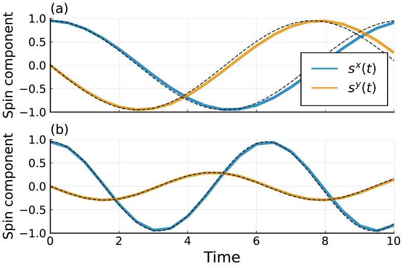
Figure 1: Numerical accuracy of integrated dipole trajectories for a single-spin Hamiltonian with an easy-axis anisotropy, $D=-1$. A large time step, $\Delta t=0.5$, is selected to emphasize error. (a) LLD using the Schrödinger midpoint method in the spin-$\frac{1}{2}$ representation. (b) The quantum mechanically correct GSD, using the Schrödinger midpoint method applied to an $S=1$ spin (i.e., $N=3$). Dashed black lines indicate reference trajectories given in Eqs. (50) and Eq. (51).

In the single-site limit, the GSD describes the exact quantum evolution of expectation values. The trajectory for a single $S=1$ spin has been given analytically in Ref. Zhang and Batista, 2021. For our pure dipole initial condition, the dipole part of the trajectory is

$$\mathbf{s}^{\mathrm{GSD}}(t)=\left[\begin{array}[]{c}s^{x}_{0}\cos(\omega^{\mathrm{GSD}}t)\\ s^{x}_{0}s^{z}_{0}\sin(\omega^{\mathrm{GSD}}t)\\ s^{z}_{0}\end{array}\right].$$ (51)

Like the dipole-only approximation, we again find precession, but here the frequency $\omega^{\mathrm{GSD}}=D$ is independent of the initial angle $\theta$. The $y$-component of the dipole is reduced by the factor $s^{z}_{0}$, such that the total spin dipole magnitude is no longer a constant of motion. This implies that weight oscillates between the three dipole and five quadrupole components of generalized spin $\mathbf{n}(t)$, and this effect is enhanced when the $z$-component of the spin is small. Recall that the quadratic Casimir $|\mathbf{n}(t)|^{2}$ is a constant of motion.

Figure 1 illustrates the numerical integration of the LLD and GSD trajectories using the Schrödinger midpoint method for spin-$\frac{1}{2}$ and spin-1 respectively, and $\theta=2\pi/5$. A fairly large integration time-step $\Delta t=0.5$ was selected to emphasize numerical error. For LLD, the spherical midpoint method McLachlan et al. (2017) is also applicable, and we observed its error to be about 2 times smaller (not shown). In all cases tested, energy conservation appears to be numerically exact under the Schrödinger midpoint integration scheme.

IV.3 Dynamics of a spin chain

Next, we study a chain of $L=100$ spins with periodic boundary conditions, and a ferromagnetic Heisenberg interaction $J=-1$. We follow Ref. Viviani, 2020 and select an initial state consisting of smoothly varying pure spin dipoles,

$$\mathbf{s}_{i}=\left[\begin{array}[]{c}\cos(2\pi x_{i}^{2})\sin(2\pi x_{i}^{3})\\ \sin(2\pi x_{i}^{2})\sin(2\pi x_{i}^{3})\\ \cos(2\pi x_{i}^{3})\end{array}\right]$$ (52)

where $x_{i}=(i-1)/99$ for indices $i=1\dots 100$.

IV.3.1 Dynamics of a pure Heisenberg chain

In the absence of the anisotropy term, $D=0$, the classical Hamiltonian is purely a function of the spin dipole, and the LLD and GSD coincide.

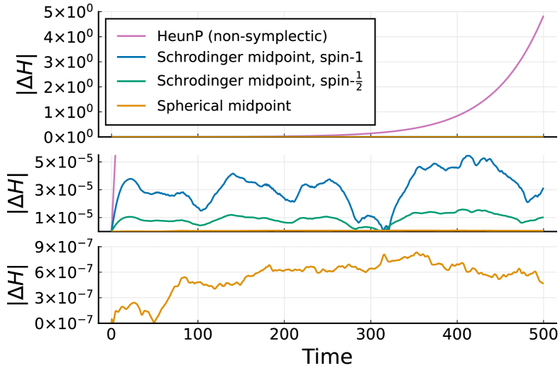
Figure 2: Energy fluctuations $\Delta H=H(t)-H(0)$ for the numerically integrated LLD of a pure Heisenberg spin chain, $J=-1$, absent anisotropy, $D=0$. We compare the following integration methods: the HeunP method applied to the Schrödinger equation, the Schrödinger midpoint method in the spin-$\frac{1}{2}$ and spin-1 representations, and the spherical midpoint method. The integration time-step is $\Delta t=0.1$. The same data is plotted on three different energy scales to illustrate the huge variation between the integration schemes for this special model.

Figure 2 illustrates the approximate conservation of energy for the various integration schemes applicable. Note that the Schrödinger midpoint method and the spherical midpoint method are both symplectic, and therefore prevent energy drift over large time-scales. In contrast, the HeunP scheme is non-symplectic, and exhibits a large, unphysical energy drift. Finally, we remark that the Schrödinger midpoint result with spin-1 precisely reproduces the curve shown in the top panel of the fourth figure in Ref. Viviani, 2020. To reproduce the bottom panel, we needed to integrate the spherical midpoint trajectory backwards in time.

IV.3.2 LLD including easy-axis anisotropy

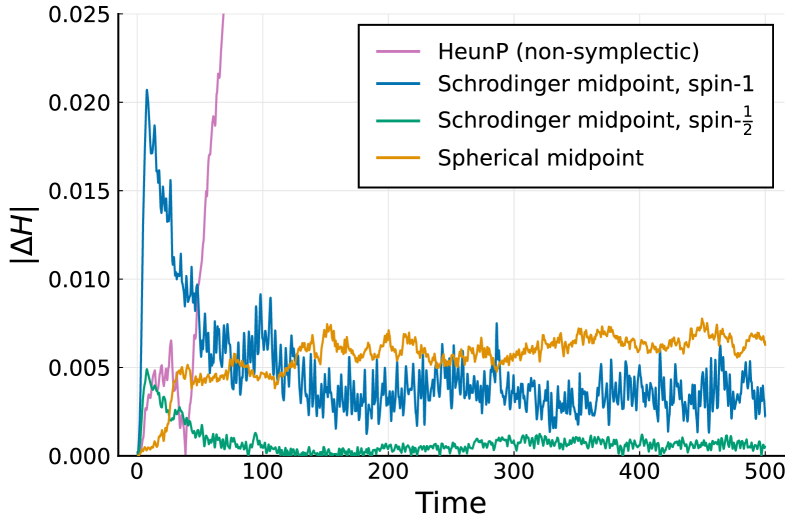
Figure 3: Energy fluctuations for the numerically integrated LLD of a Heisenberg spin chain with $J=-1$, now including an easy-axis anisotropy, $D=-1$. The numerical integration schemes are the same as in Fig. 2, but here we use a much smaller integration time-step, $\Delta t=0.02$.

We now include an easy-axis anisotropy, $D=-1$, in the Heisenberg chain. With this additional term, the LLD and GSD classical limits deviate. First we will consider the LLD case.

Figure 3 compares accuracy of four integration schemes. Relative to the $D=0$ case in Fig. 2, we observe much larger energy fluctuations, despite a significantly smaller time-step of $\Delta t=0.02$ (down from $\Delta t=0.1$). Energy fluctuations observed from the Schrödinger midpoint and spherical midpoint numerical integration schemes are now of the same order. In all cases tested, when applying the Schrödinger midpoint method to the LLD, the spin-$\frac{1}{2}$ representation is preferred over the spin-1 representation. There remains a tremendous advantage in using a symplectic integration scheme—the energy of the HeunP method continues to drift strongly.

IV.3.3 GSD including easy-axis anisotropy

Our final numerical benchmark is the Heisenberg spin chain with easy-axis anisotropy $D=-1$ using the generalized spin dynamics. Here we must work with all three levels of the $S=1$ spins, which give rise to both dipole and quadrupole moments, and the traditional LLD numerical integration schemes do not apply.

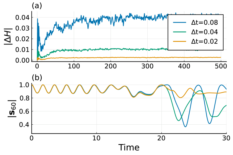
Figure 4: (a) Energy fluctuations for the numerically integrated GSD of a Heisenberg spin chain with $S=1$, $J=-1$ and easy-axis anisotropy, $D=-1$. We use the Schrödinger midpoint method with varying time-step $\Delta t$. (b) Time evolution of the dipole magnitude $|\mathbf{s}_{i}|$ for site index $i=60$.

Figure 4 shows time integration using the Schrödinger midpoint method. The top panel illustrates that the energy fluctuations decrease approximately quadratically with time-step $\Delta t$, consistent with the second order accuracy of the implicit midpoint method Hairer et al. (2006). The bottom panel shows the time evolution of the dipole magnitude $|\mathbf{s}_{i}|$ for site index $i=60$. Fluctuations in the dipole magnitude are possible because weight can be transferred to the quadrupole part of the generalized spins $\mathbf{n}_{i}$. All spins in the initial configuration, Eq. (52), are pure dipoles, with a relatively slow variation along the spin chain. Therefore the initial dynamics is reasonably well approximated by the single spin limit, $J\approx 0$, previously considered in Fig. 1. At times $t\gtrsim 10$, however, high-frequency spatial variations in the spin chain propagate to site $i=60$. At this point, chaotic dynamics can be observed, and the three trajectories integrated using different $\Delta t$ quickly separate. As expected for a symplectic integrator, no significant energy drift is observed over arbitrarily long trajectory lengths.

V Conclusions

We have presented a numerical integration scheme, the Schrödinger midpoint method, that applies to the generalized spin dynamics, Eq. (3). In the special case of the Landau-Lifshitz dynamics, Eq. (1), this method reduces to previously known symplectic integrators McLachlan et al. (2015); Viviani (2020). The Schrödinger midpoint method can be viewed as a special case of the Isospectral Midpoint Method Modin and Viviani (2020); Viviani (2020), which applies to general Lie-Poisson systems. Compared to IMM, our approach is specialized to Eq. (3), which arises as a classical limit of quantum mechanics, and has the numerical advantage of describing the evolution of a single eigenvector vector (the coherent spin state) rather than that of a full matrix. The method exactly respects the local symplectic structure of the Lie-Poisson system, or equivalently, the global symplectic structure of the Schrödinger equation, which may be understood as a canonical Hamiltonian system. We anticipate that this method will be of broad applicability to the study of spin $S>\frac{1}{2}$ systems with strong single-ion anisotropy, for which the spin quadrupole (and perhaps higher-order) moments cannot be ignored Zhang and Batista (2021); Bai et al. (2021); Akagi et al. (2021); Remund et al. (2022); Amari et al. (2022); Zhang et al. (2022).

Code availability

Code to reproduce all plots is available online at https://github.com/SunnySuite/SchrodingerMidpoint.jl. The methods we present are also implemented in Sunny, an open-source code for simulating general spin systems sun (2022).

Appendix A Spin operators as representations of SU(2)

Here we review some properties of the irreducible representations of SU(2), which serve as quantum spin operators. The SU(2) irreps are conventionally labeled by a spin index $S\in\{\frac{1}{2},1,\frac{3}{2},\dots\}$, and have dimension $N=2S+1$.

For spin $S=1/2$, a conventional basis for the spin matrices is $S^{\alpha}=\sigma^{\alpha}/2$, where $\sigma^{\alpha}$ are the Pauli matrices,

$$S^{x}=\frac{1}{2}\left[\begin{array}[]{cc}0&1\\ 1&0\end{array}\right],\,S^{y}=\frac{1}{2}\left[\begin{array}[]{cc}0&-\mathrm{i}\\ \mathrm{i}&0\end{array}\right],\,S^{z}=\frac{1}{2}\left[\begin{array}[]{cc}1&0\\ 0&-1\end{array}\right].$$ (53)

More generally, it is convenient to work in a basis with $S^{z}$ diagonal. For spin $S=1$,

$$S^{x}=\frac{1}{\sqrt{2}}\left[\begin{array}[]{ccc}0&1&0\\ 1&0&1\\ 0&1&0\end{array}\right],\,S^{y}=\frac{1}{\sqrt{2}}\left[\begin{array}[]{ccc}0&-\mathrm{i}&0\\ \mathrm{i}&0&-\mathrm{i}\\ 0&\mathrm{i}&0\end{array}\right],\,S^{z}=\left[\begin{array}[]{ccc}1&0&0\\ 0&0&0\\ 0&0&-1\end{array}\right].$$ (54)

This pattern generalizes to arbitrary spin $S$,

$$S^{x}=\left[\begin{array}[]{cccc}0&a_{1}\\ a_{1}&0&\ddots\\ &\ddots&\ddots&a_{N-1}\\ &&a_{N-1}&0\end{array}\right],\,S^{y}=\left[\begin{array}[]{cccc}0&-\mathrm{i}\,a_{1}\\ \mathrm{i}\,a_{1}&0&\ddots\\ &\ddots&\ddots&-\mathrm{i}\,a_{N-1}\\ &&\mathrm{i}\,a_{N-1}&0\end{array}\right],\,S^{z}=\left[\begin{array}[]{cccc}S\\ &S-1\\ &&\ddots\\ &&&-S\end{array}\right],$$ (55)

where the off-diagonal elements, $a_{j}=\frac{1}{2}\sqrt{2(S+1)j-j(j+1)},$ satisfy the symmetry $a_{j}=a_{N-j}$. These coefficients also enter into raising and lowering operators, defined as $S_{\pm}=S^{x}\pm iS^{y}$.

The spin matrices $S^{\alpha}$ define the action of the quantum spin operators. The many-body spin operator $\hat{S}_{i}^{\alpha}$ is defined to act only on the $i$th local Hilbert space,

$$\hat{S}_{i}^{\alpha}=\underset{\textrm{$i$th term}}{\underbrace{I\otimes\dots\otimes\hat{S}^{\alpha}}}\otimes\dots\otimes I.$$

The local operator $\hat{S}^{\alpha}$ is defined by its action $\langle e_{a}|$$\hat{S}^{\alpha}|e_{b}\rangle=(S^{\alpha})_{ab}$ in some basis $|e_{1}\rangle,\dots,|e_{N}\rangle$. The operators $\hat{S}_{i}^{\alpha}$ share all mathematical properties of the matrices $S^{\alpha}$, to be listed below.

By construction, the spin matrices satisfy the commutation relations,

$$[S^{\alpha},S^{\beta}]=\mathrm{i}\,\epsilon_{\alpha\beta\gamma}S^{\gamma},$$ (56)

which gives rise to the same commutation relations, Eq. (2), for the quantum spin operators.

The $N$ eigenvalues for each spin matrix $S^{\alpha}$ run from $m=-S,\dots,S$. The total angular momentum for each spin $i$ is scalar, i.e.,

$$|\mathbf{S}|^{2}=(S^{x})^{2}+(S^{y})^{2}+(S^{z})^{2}=S(S+1)I,$$ (57)

with $I$ the identity matrix. This polynomial is the sole Casimir of $\mathfrak{su}(2)$.

The spin matrices satisfy the orthonormality condition

$$\mathrm{tr}\,S^{\alpha}S^{\beta}=\tau\delta_{\alpha\beta},$$ (58)

which is a special case of Eq. (9). The normalization constant is the sum of squares of eigenvalues,

$$\tau=\sum_{m=-S}^{S}m^{2}=\frac{2}{3}S\left(S+\frac{1}{2}\right)(S+1).$$ (59)

Appendix B Review of generalized spin dynamics

Following Ref. Zhang and Batista, 2021, we here review how Eq. (3) emerges as a classical limit of a many-body quantum system.

Consider a many-body quantum spin Hamiltonian $\hat{\mathcal{H}}$, such as the spin chain model of Eq. (42). This Hamiltonian may involve spin operators $\hat{S}^{\alpha}$ with spin representation $S$, corresponding to local Hilbert space dimension $N=2S+1$. The choice $S>1/2$ would be appropriate to model, e.g., the effective spin angular momentum associated with a collection of spins that have aligned according to Hund’s rules.

For $N>2$, the Hamiltonian may include local anisotropy terms, such as $(\hat{S}_{i}^{z})^{2}$. Such terms are not a linear combination of the $\hat{S}_{i}^{\alpha}$, i.e., do not generate usual rotations of the local spin state. Importantly, however, any local physical operator can be decomposed as a linear combination of the $N^{2}-1$ generators $\hat{T}_{i}^{\alpha}$ of SU($N$) in the fundamental representation, plus a constant shift.

Using the completeness of the generators $\hat{T}_{i}^{\alpha}$ in each local Hilbert space, we can write a general Hamiltonian as a polynomial expansion,

$$\hat{\mathcal{H}}=\sum_{i}J_{(i,\alpha)}^{(1)}\hat{T}_{i}^{\alpha}+\frac{1}{2}\sum_{i,j}J_{(i,\alpha),(j,\beta)}^{(2)}\hat{T}_{i}^{\alpha}\hat{T}_{j}^{\beta}+\dots,$$ (60)

up to an irrelevant constant shift. Recall that summation over repeated Greek indices is implied.

Any coefficient $J_{[\dots]}^{(n)}$ that couples a site with itself (e.g., a single-ion anisotropy term) can be effectively absorbed into lower order coefficients $J_{[\dots]}^{(n-1)}$ by the completeness of the generators $\hat{T}_{i}^{\alpha}$ for each site $i$. Therefore, without loss of generality, we require that the coefficients couple only distinct sites, e.g.,

$$J_{(i,\alpha),(j,\beta)}^{(2)} \propto(1-\delta_{ij}).$$ (61)

Since $\hat{T}_{i}^{\alpha}$ and $\hat{T}_{j}^{\beta}$ commute for $i\neq j$, we also have freedom to symmetrize the coefficients, e.g.,

$$J_{(i,\alpha),(j,\beta)}^{(2)}=J_{(j,\beta),(i,\alpha)}^{(2)}.$$ (62)

The Hamiltonian $\hat{\mathcal{H}}$ determines the evolution of a general quantum state,

$$\frac{\mathrm{d}}{\mathrm{d}t}|\psi\rangle=e^{-\mathrm{i}\,t\hat{\mathcal{H}}}|\psi\rangle,$$ (63)

where we take $\hbar=1$. The time evolution of an arbitrary expectation value $\langle\hat{A}\rangle=\langle\psi|\hat{A}|\psi\rangle$ follows,

$$\mathrm{i}\,\frac{\mathrm{d}}{\mathrm{d}t}\langle\hat{A}\rangle=\langle[\hat{A},\hat{\mathcal{H}}]\rangle.$$ (64)

To take the classical limit, we will ignore quantum entanglement and approximate the time-evolving many-body state $|\psi\rangle$ as a tensor product of coherent states of a given algebra,

$$|\psi\rangle\approx|Z\rangle=\bigotimes_{i=1}^{L}|Z_{i}\rangle.$$ (65)

In the remainder of this section, our purpose is to demonstrate the following: This approximation yields a self-consistent and closed dynamics on local expectation values, namely, Eq. (3).

Product states allow the factorization of expectation values over distinct sites,

$$\langle Z|\hat{T}_{i}^{\alpha}\hat{T}_{j}^{\beta}|Z\rangle=n_{i}^{\alpha}n_{j}^{\beta}.$$ (66)

It follows that, under the assumption of Eq. (65), the expected energy $H=\langle\hat{\mathcal{H}}\rangle$ is

$$H=\sum_{i}J_{(i,\alpha)}^{(1)}n_{i}^{\alpha}+\frac{1}{2}\sum_{i,j}J_{(i,\alpha),(j,\beta)}^{(2)}n_{i}^{\alpha}n_{j}^{\beta}+\dots$$ (67)

In other words, substituting $\hat{T}_{i}^{\alpha}\rightarrow n_{i}^{\alpha}$ in the quantum Hamiltonian $\hat{\mathcal{H}}$ yields the classical Hamiltonian $H$.

Inserting the general Hamiltonian of Eq. (60) into the dynamics Eq. (64) for a local operator $\hat{A}=\hat{A}_{k}$ yields,

$$\mathrm{i}\,\frac{\mathrm{d}}{\mathrm{d}t}\langle\hat{A}_{k}\rangle =\sum_{i}J_{(i,\alpha)}^{(1)}\langle[\hat{A}_{k},\hat{T}_{i}^{\alpha}]\rangle$$

$$\quad+\frac{1}{2}\sum_{i,j}J_{(i,\alpha),(j,\beta)}^{(2)}\langle[\hat{A}_{k},\hat{T}_{i}^{\alpha}\hat{T}_{j}^{\beta}]\rangle+\dots$$ (68)

For the first term, we use

$$\sum_{i}J_{(i,\alpha)}^{(1)}[\hat{A}_{k},\hat{T}_{i}^{\alpha}]=J_{(k,\alpha)}^{(1)}[\hat{A}_{k},\hat{T}_{k}^{\alpha}].$$ (69)

For the second term, Eq. (61) ensures $i\neq j$, and we require either $k=i$ or $k=j$. It follows,

$$\frac{1}{2}\sum_{i,j} J_{(i,\alpha),(j,\beta)}^{(2)}[\hat{A}_{k},\hat{T}_{i}^{\alpha}\hat{T}_{j}^{\beta}]$$

$$=\frac{1}{2}[\hat{A}_{k},\hat{T}_{k}^{\alpha}]\sum_{j}\left(J_{(k,\alpha),(j,\beta)}^{(2)}\hat{T}_{j}^{\beta}+J_{(j,\alpha),(k,\beta)}^{(2)}\hat{T}_{j}^{\alpha}\right)$$

$$=[\hat{A}_{k},\hat{T}_{k}^{\alpha}]\sum_{j}J_{(k,\alpha),(j,\beta)}^{(2)}\hat{T}_{j}^{\beta}.$$ (70)

In the second step, we used the symmetrization convention of Eq. (62). Combining results, and using again the approximation Eq. (65) to factorize the expectation values on distinct sites, we find

$$\mathrm{i}\,\frac{\mathrm{d}}{\mathrm{d}t}\langle\hat{A}_{k}\rangle=\langle[\hat{A}_{k},\hat{T}_{k}^{\alpha}]\rangle\Big{(}J_{(k,\alpha)}^{(1)}+\sum_{j}J_{(k,\alpha),(j,\beta)}^{(2)}\langle\hat{T}_{j}^{\beta}\rangle+\dots\Big{)}.$$ (71)

The second factor on the right-hand side is $\partial H/\partial n_{k}^{\alpha}$, and this result holds to all expansion orders. Relabeling $(k,\alpha)\rightarrow(i,\beta)$, the result is

$$\mathrm{i}\,\frac{\mathrm{d}}{\mathrm{d}t}\langle\hat{A}_{i}\rangle=\langle[\hat{A}_{i},\hat{T}_{i}^{\beta}]\rangle\frac{\partial H}{\partial n_{i}^{\beta}},$$ (72)

which is valid for any local operator $\hat{A}_{i}$. Selecting $\hat{A}_{i}=\hat{T}_{i}^{\alpha}$ and using Eq. (4), we reproduce the generalized spin dynamics, Eq. (3),

$$\frac{\mathrm{d}}{\mathrm{d}t}n_{i}^{\alpha}=f_{\alpha,\beta,\gamma}\frac{\partial H}{\partial n_{i}^{\beta}}n_{i}^{\gamma}.$$ (73)

Although we motivated the form of $\hat{\mathcal{H}}$ in Eq. (60) using the language of spin systems, this Hamiltonian is in fact fully general. We could have taken each local Hilbert space $i$ to represent, e.g., a tensor product space of multiple quantum spins. The time evolution of classical expectation values, Eq. (73), would then capture quantum entanglement effects within each local Hilbert space.

Appendix C Hamiltonian structure of the Schrödinger equation

Each $\mathfrak{su}(N)$ generator can be decomposed into its purely real and imaginary parts,

$$T^{\alpha}=A^{\alpha}+\mathrm{i}\,B^{\alpha}.$$ (74)

Because $T^{\alpha}$ is Hermitian, it follows that $A^{\alpha}$ and $B^{\alpha}$ are symmetric and antisymmetric, respectively.

Substituting this decomposition into the Schrödinger equation of Eq. (5), we find

$$\frac{\mathrm{d}}{\mathrm{d}t}\mathbf{Z}_{i}=\frac{\partial H}{\partial n_{i}^{\alpha}}\left(-\mathrm{i}\,A^{\alpha}+B^{\alpha}\right)\mathbf{Z}_{i}.$$ (75)

Decomposing the state vector into real and imaginary parts,

$$\mathbf{Z}_{i}=\frac{1}{\sqrt{2}}\left(\mathbf{p}_{i}-\mathrm{i}\,\mathbf{q}_{i}\right),$$ (76)

allows formulation of the Schrödinger equation as an entirely real dynamics,

$$\frac{\mathrm{d}\mathbf{p}_{i}}{\mathrm{d}t} =\frac{\partial H}{\partial n_{i}^{\alpha}}\left(-A^{\alpha}\mathbf{q}_{i}+B^{\alpha}\mathbf{p}_{i}\right)$$ (77)

$$\frac{\mathrm{d}\mathbf{q}_{i}}{\mathrm{d}t} =\frac{\partial H}{\partial n_{i}^{\alpha}}\left(A^{\alpha}\mathbf{p}_{i}+B^{\alpha}\mathbf{q}_{i}\right).$$ (78)

Expectation values $n_{i}^{\alpha}=\mathbf{Z}_{i}^{\dagger}T^{\alpha}\mathbf{Z}_{i}$ may be written,

$$n_{i}^{\alpha} =\frac{1}{2}\left(\mathbf{p}_{i}-\mathrm{i}\,\mathbf{q}_{i}\right)^{\dagger}T^{\alpha}\left(\mathbf{p}_{i}-\mathrm{i}\,\mathbf{q}_{i}\right).$$ (79)

Expanding the right-hand side, and decomposing $T^{\alpha}$ into its symmetric and antisymmetric parts, we find

$$n_{i}^{\alpha} =\frac{1}{2}\mathbf{p}_{i}^{T}A^{\alpha}\mathbf{p}_{i}+\frac{1}{2}\mathbf{q}_{i}^{T}A^{\alpha}\mathbf{q}_{i}$$

$$\quad\quad-\frac{1}{2}\mathbf{q}_{i}^{T}B^{\alpha}\mathbf{p}_{i}+\frac{1}{2}\mathbf{p}_{i}^{T}B^{\alpha}\mathbf{q}_{i}.$$ (80)

Differentiation yields

$$\frac{\partial n_{i}^{\alpha}}{\partial\mathbf{p}_{i}} =A^{\alpha}\mathbf{p}_{i}+B^{\alpha}\mathbf{q}_{i}$$ (81)

$$\frac{\partial n_{i}^{\alpha}}{\partial\mathbf{q}_{i}} =A^{\alpha}\mathbf{q}_{i}-B^{\alpha}\mathbf{p}_{i}.$$ (82)

Energy derivatives can now be evaluated. Using the chain rule,

$$\frac{\partial H}{\partial\mathbf{p}_{i}} =\frac{\partial H}{\partial n_{i}^{\alpha}}\left(A^{\alpha}\mathbf{p}_{i}+B^{\alpha}\mathbf{q}_{i}\right)$$ (83)

$$\frac{\partial H}{\partial\mathbf{q}_{i}} =\frac{\partial H}{\partial n_{i}^{\alpha}}\left(A^{\alpha}\mathbf{q}_{i}-B^{\alpha}\mathbf{p}_{i}\right).$$ (84)

Inserting these results into Eqs. (77) and (78), we find that the Schrödinger equation is described by Hamilton’s equations of motion,

$$\frac{\mathrm{d}\mathbf{p}_{i}}{\mathrm{d}t}=-\frac{\partial H}{\partial\mathbf{q}_{i}},\quad\frac{\mathrm{d}\mathbf{q}_{i}}{\mathrm{d}t}=+\frac{\partial H}{\partial\mathbf{p}_{i}}.$$ (85)

Appendix D Derivation of the Schrödinger midpoint formulas for LLD

In this Appendix, we derive the results stated in Sec. III.2. The LLD of spin dipoles, Eq. (1), may be formulated as a Schrödinger dynamics, Eq. (5), involving generators $S^{\alpha}$ of SU(2) in some representation. The midpoint method applied to the Schrödinger dynamics can be interpreted as two half time-steps, Eq. (32) and (33). Consider the former, from which we determine

$$s_{i}^{\alpha}=\tilde{\mathbf{Z}}_{i}^{\dagger}\left(S^{\alpha}+\mathrm{i}\,\frac{\Delta t}{2}[S^{\alpha},\tilde{\mathfrak{H}}_{i}]-\frac{\Delta t^{2}}{4}\tilde{\mathfrak{H}}_{i}S^{\alpha}\tilde{\mathfrak{H}}_{i}\right)\tilde{\mathbf{Z}}_{i},$$ (86)

where $s^{\alpha}_{i}=\mathbf{Z}_{i}^{\dagger}S^{\alpha}\mathbf{Z}_{i}$.

The first term is an expectation value, $\tilde{s}_{i}^{\alpha}=\tilde{\mathbf{Z}}_{i}^{\dagger}S^{\alpha}\tilde{\mathbf{Z}}_{i}$. The second term may be expanded using Eqs. (6) and (56),

$$\mathrm{i}\,[S^{\alpha},\tilde{\mathfrak{H}}]=\mathrm{i}\,\frac{\partial H}{\partial\tilde{s}_{i}^{\beta}}[S^{\alpha},S^{\beta}]=-\epsilon_{\alpha\beta\gamma}\frac{\partial H}{\partial\tilde{s}^{\beta}_{i}}S^{\gamma}.$$ (87)

In vector notation,

$$\mathrm{i}\,\tilde{\mathbf{Z}}_{i}^{\dagger}[\mathbf{S},\tilde{\mathfrak{H}}]\tilde{\mathbf{Z}}_{i}=\tilde{\mathbf{s}}_{i}\times\frac{\partial H}{\partial\tilde{\mathbf{s}}_{i}}.$$ (88)

To evaluate the third term, we must incorporate more information about the matrix representation of the generators $S^{\alpha}$. Let us introduce the notation,

$$\tilde{\mathfrak{H}}_{i}=\frac{\partial H}{\partial\tilde{s}^{\beta}_{i}}S^{\beta}=\mathbf{a}\cdot\mathbf{S}$$ (89)

In the special cases of the spin-$\frac{1}{2}$ and spin-1 representations, the matrix spin operators satisfy

$$(\mathbf{a}\cdot\mathbf{S})\mathbf{S}(\mathbf{a}\cdot\mathbf{S})=\begin{cases}\frac{\mathbf{a}(\mathbf{a}\cdot\mathbf{S})}{2}-\frac{|\mathbf{a}|^{2}\mathbf{S}}{4}&\textrm{(spin-$\frac{1}{2}$)}\\ \mathbf{a}(\mathbf{a}\cdot\mathbf{S})&\textrm{(spin-1)}\end{cases},$$ (90)

valid for any $\mathbf{a}\in\mathbb{R}^{3}$.

It follows,

$$\tilde{\mathfrak{H}}\mathbf{S}\tilde{\mathfrak{H}}=\begin{cases}\frac{1}{2}\frac{\partial H}{\partial\tilde{\mathbf{s}}_{i}}\left(\frac{\partial H}{\partial\tilde{\mathbf{s}}_{i}}\cdot\mathbf{S}\right)-\frac{1}{4}\left|\frac{\partial H}{\partial\tilde{\mathbf{s}}_{i}}\right|^{2}\mathbf{S}&\textrm{(spin-$\frac{1}{2}$)}\\ \frac{\partial H}{\partial\tilde{\mathbf{s}}_{i}}\left(\frac{\partial H}{\partial\tilde{\mathbf{s}}_{i}}\cdot\mathbf{S}\right)&\textrm{(spin-1)}\end{cases}.$$ (91)

Inserting these results into Eq. (86) yields Eq. (34). A similar argument yields Eq. (35). Combined, these equations provide a closed-form update rule entirely in terms of the spin dipoles.

References

- Zhang and Batista (2021) H. Zhang and C. D. Batista, Phys. Rev. B 104, 104409 (2021).
- Zapf et al. (2006) V. S. Zapf, D. Zocco, B. R. Hansen, M. Jaime, N. Harrison, C. D. Batista, M. Kenzelmann, C. Niedermayer, A. Lacerda, and A. Paduan-Filho, Phys. Rev. Lett. 96, 077204 (2006).
- Do et al. (2021) S.-H. Do, H. Zhang, T. J. Williams, T. Hong, V. O. Garlea, J. Rodriguez-Rivera, T.-H. Jang, S.-W. Cheong, J.-H. Park, C. D. Batista, et al., Nature communications 12, 1 (2021).
- Bai et al. (2021) X. Bai, S.-S. Zhang, Z. Dun, H. Zhang, Q. Huang, H. Zhou, M. B. Stone, A. I. Kolesnikov, F. Ye, C. D. Batista, and M. Mourigal, Nat. Phys. 17, 467 (2021).
- Jaime et al. (2004) M. Jaime, V. F. Correa, N. Harrison, C. D. Batista, N. Kawashima, Y. Kazuma, G. A. Jorge, R. Stern, I. Heinmaa, S. A. Zvyagin, Y. Sasago, and K. Uchinokura, Phys. Rev. Lett. 93, 087203 (2004).
- Qiu et al. (2005) Y. Qiu, C. Broholm, S. Ishiwata, M. Azuma, M. Takano, R. Bewley, and W. J. L. Buyers, Phys. Rev. B 71, 214439 (2005).
- Okamoto et al. (2013) Y. Okamoto, G. J. Nilsen, J. P. Attfield, and Z. Hiroi, Phys. Rev. Lett. 110, 097203 (2013).
- Marsden and Ratiu (1999) J. E. Marsden and T. S. Ratiu, Introduction to Mechanics and Symmetry, A Basic Exposition of Classical Mechanical Systems, Texts in Applied Mathematic, Vol. 17 (Springer Berlin Heidelberg, 1999).
- McLachlan et al. (2015) R. I. McLachlan, K. Modin, and O. Verdier, IMA Journal of Numerical Analysis 35, 546 (2015).
- Modin and Viviani (2020) K. Modin and M. Viviani, Found Comput Math 20, 889 (2020).
- Viviani (2020) M. Viviani, Bit Numer Math 60, 741 (2020).
- Engø and Faltinsen (2001) K. Engø and S. Faltinsen, SIAM J. Numer. Anal. 39, 128 (2001).
- Hairer et al. (2006) E. Hairer, C. Lubich, and G. Wanner, Geometric Numerical Integration: Structure-Preserving Algorithms for Ordinary Differential Equations, Springer Series in Computational Mathematics, Vol. 31 (Springer Berlin Heidelberg, 2006).
- Huberman et al. (2008) T. Huberman, D. A. Tennant, R. A. Cowley, R. Coldea, and C. D. Frost, Journal of Statistical Mechanics: Theory and Experiment 2008, P05017 (2008).
- Iserles et al. (2000) A. Iserles, H. Z. Munthe-Kaas, S. P. Nørsett, and A. Zanna, Acta Numerica 9, 215 (2000).
- Iserles and Quispel (2016) A. Iserles and G. R. W. Quispel, arXiv:1602.07755 [math] (2016), arXiv:1602.07755 [math] .
- Munthe-Kaas (1998) H. Munthe-Kaas, Bit Numer Math 38, 92 (1998).
- Zhong and Marsden (1988) G. Zhong and J. E. Marsden, Physics Letters A 133, 134 (1988).
- Channell and Scovel (1991) P. J. Channell and J. C. Scovel, Physica D: Nonlinear Phenomena 50, 80 (1991).
- McLachlan (1993) R. I. McLachlan, Phys. Rev. Lett. 71, 3043 (1993).
- McLachlan and Scovel (1995) R. I. McLachlan and C. Scovel, J Nonlinear Sci 5, 233 (1995).
- Krech et al. (1998) M. Krech, A. Bunker, and D. P. Landau, Computer Physics Communications 111, 1 (1998).
- Omelyan et al. (2001) I. P. Omelyan, I. M. Mryglod, and R. Folk, Phys. Rev. Lett. 86, 898 (2001).
- Tranchida et al. (2018) J. Tranchida, S. J. Plimpton, P. Thibaudeau, and A. P. Thompson, Journal of Computational Physics 372, 406 (2018).
- McLachlan et al. (2014) R. I. McLachlan, K. Modin, and O. Verdier, Phys. Rev. E 89, 061301 (2014).
- McLachlan et al. (2017) R. McLachlan, K. Modin, and O. Verdier, Math. Comp. 86, 2325 (2017).
- Skubic et al. (2008) B. Skubic, J. Hellsvik, L. Nordström, and O. Eriksson, J. Phys.: Condens. Matter 20, 315203 (2008).
- Mentink et al. (2010) J. H. Mentink, M. V. Tretyakov, A. Fasolino, M. I. Katsnelson, and T. Rasing, J. Phys.: Condens. Matter 22, 176001 (2010).
- Akagi et al. (2021) Y. Akagi, Y. Amari, N. Sawado, and Y. Shnir, Phys. Rev. D 103, 065008 (2021), arXiv:2101.10566 .
- Remund et al. (2022) K. Remund, R. Pohle, Y. Akagi, J. Romhányi, and N. Shannon, arXiv:2203.09819 [cond-mat] (2022), arXiv:2203.09819 [cond-mat] .
- Amari et al. (2022) Y. Amari, Y. Akagi, S. B. Gudnason, M. Nitta, and Y. Shnir, arXiv:2204.01476 [cond-mat, physics:hep-th] (2022), arXiv:2204.01476 [cond-mat, physics:hep-th] .
- Zhang et al. (2022) H. Zhang, Z. Wang, D. Dahlbom, K. Barros, and C. D. Batista, arXiv:2203.15248 [cond-mat] (2022), arXiv:2203.15248 [cond-mat] .
- sun (2022) (2022), https://github.com/SunnySuite/Sunny.jl/.