Quantum coherence controls the nature of equilibration in coupled chaotic systems

Abstract

A bipartite system whose subsystems are fully quantum chaotic and coupled by a perturbative interaction with a tunable strength is a paradigmatic model for investigating how isolated quantum systems relax towards an equilibrium. It is found that quantum coherence of the initial product states in the uncoupled eigenbasis can be viewed as a resource for equilibration and approach to thermalization as manifested by the entanglement. Results are given for four distinct perturbation strength regimes, the ultra-weak, weak, intermediate, and strong regimes. For each, three types of initially unentangled states are considered, coherent random-phase superpositions, random superpositions, and eigenstate products. A universal time scale is identified involving the interaction strength parameter. Maximally coherent initial states thermalize for any perturbation strength in spite of the fact that in the ultra-weak perturbative regime the underlying eigenstates of the system have a tensor product structure and are not at all thermal-like; though the time taken to thermalize tends to infinity as the interaction vanishes. In contrast to the widespread linear behavior, in this regime the entanglement initially grows quadratically in time.

I Introduction

Thermalization in isolated quantum many-body systems has been an active area of research for many years [1]. The essential question is whether the system prepared in some initial state of interest reaches a thermal equilibrium after a sufficiently long time. As proposed roughly three decades ago [2, 3], thermalization really happens at the eigenstate level and is indicative of quantum chaotic nature of the system under consideration. Thus, the system relaxes to a thermal state irrespective of the initial state and without having to do any initial state ensemble averaging. This thermalization is seen in the subsystem states of such isolated systems where the reduced density matrix of the subsystem follows quantum statistical mechanics [3]. There are numerous contemporary studies on the process of thermalization in isolated quantum many-body systems and for different classes of initial states [4, 5, 6, 7, 8, 9, 10]. Whereas any lack of thermalization is often attributed to disorder induced many-body localization [9], it may originate from memory effects in the initial state purely from weakness of the interactions [11].

Compelling insights pertaining to the foundations of quantum statistical mechanics can be gained through the study of paradigmatic bipartite systems whose subsystems are quantum chaotic. By adding an interaction between the subsystems with a tunable strength, relaxation towards an equilibrium in the full system of various classes of initial states can be studied over the complete range from vanishing interactions to the opposite limit of extremely strong interactions. There are classes of initially unentangled (product) states of such subsystems that respond quite differently to weak interaction strengths. Some may thermalize achieving near maximal entanglement as random states, others may equilibrate but with smaller entanglement, whereas others practically develop no entanglement at all.

In this context, taking advantage of the universality of chaotic single-particle or many-body dynamics, a random matrix model that highlights some of the major scenarios in the case of bipartite weakly coupled chaotic systems is explored analytically and numerically. In particular, three sets of unentangled initial pure states constructed from the subsystem eigenstates in the absence of interactions are contrasted: (i) tensor products of coherent random-phase superpositions (C $\otimes$ C type), (ii) tensor products of random superpositions (R $\otimes$ R type), and (iii) tensor product of individual subsystem eigenstates (E $\otimes$ E type). In each of these cases, when interactions are turned on, the interest is in studying the entanglement production and its time scale, its long-time average, and the nature of the fluctuations. Naturally the interaction strength plays a crucial role and the full range is explored from the perturbative regime $\Lambda\ll 1$, to $\Lambda\gtrsim 1$ where $\Lambda$ is a scaled universal transition parameter identified earlier [12, 13, 14]. In this regime, a spectral transition is observed from the Poisson to Wigner level statistics, although the subsystem dynamics is always fully chaotic.

The set (i) corresponds to an ensemble of initial states of maximal coherence [15]. Coherence in a state (represented as density matrix) is quantified by the off-diagonal elements of its density matrix and is a basis dependent notion. However, fixing a preferred basis, it has been found to be useful to develop coherence measures in quantum information theory, and states that are diagonal are incoherent. In parallel to the resource theory of entanglement, a resource theory for quantum coherence has been developed; for a review see [16]. For both sets (i) and (ii), the infinite-time averaged entanglement can be nearly maximal for arbitrarily small interactions, although the approach to the long time limit can be arbitrarily slow. It turns out that set (i) of random-phases with maximal coherence (C $\otimes$ C) engenders a large amount of entanglement, and already reaches the typical thermalized entangled state value. This occurs in spite of the perturbative nature of the interactions, i.e. $\Lambda\ll 1$ and Poissonian level statistics [17]. For the set (ii) of random superpositions (R $\otimes$ R) a smaller amount of entanglement is obtained in comparison to set (i) states. The set (iii) of subsystem eigenstate products (E $\otimes$ E) are incoherent from this point of view as they have diagonal density matrices. Under perturbative interactions, their entanglement remains essentially perturbative [18]. Thus, the results suggest investigating quantum coherence in the uncoupled eigenbasis as a “resource” for thermalization. In addition, the universal rescaled time that was identified in [18] holds true in the current study for all initial states considered.

Previous studies have shown a linear-in-time entanglement growth in systems with signatures of classical chaos [19, 20, 21, 22, 23, 24], and in many-body systems [25, 26, 27]. This study reveals that the initial entanglement growth is controlled by both the transition parameter $\Lambda$ and the quantum coherence in the initial state. The former leads to a linear growth and the latter to a quadratic one where a competition between these two is observed and a time scale is derived depicting the transition between linear and quadratic growths. In the ultra-weak regime, the linear growth is suppressed and a dominant quadratic growth is seen.

The structure of this paper is as follows: the next section briefly presents essential background regarding thermalization, quantum coherence, quantum chaos, bipartite systems, the transition parameter, and the universal rescaled time. In Sect. III, a relation is given for the infinite time averaged purity, and hence linear entropy as well, along with a summary of the four perturbation regimes. This is followed with a section on analytical and numerical results for the limiting extremes of ultra-weak and ultra-strong interaction strengths. The remaining perturbation regimes, weak and intermediate strength, are covered in Sect. V. The final section summarizes the results of this work and gives a brief outlook.

II Background

It is helpful to review key background information regarding thermalization and equilibration in isolated quantum systems, quantum coherence as a resource, bipartite systems and linear entropy, and set up notation to be used throughout the rest of the paper. Also included are the relevant random matrix transition ensembles, and the concepts of symmetry breaking, the transition parameter, and universal rescaled time.

II.1 Thermalization in isolated quantum many-body systems

An isolated many-body system prepared in an initial pure state thermalizes when evolved for a sufficiently long time if the eigenstates of the system are quantum chaotic in nature, and behave according to the eigenstate thermalization hypothesis (ETH) [2, 3]. For such systems, any generic initial state will approach thermal equilibrium in the strong sense, meaning almost all the initial states relax to equilibrium beyond some time, thus exhibiting thermal distributions such as Maxwell, or Bose-Einstein, or Fermi-Dirac depending on the exchange symmetry and stationary expectation values. In contrast to strong thermalization, weak thermalization has been found to exist in some types of initial product states [28, 29]. Weak thermalization occurs when the observable of interest fluctuates about the thermal average and only with long-time averaging gives the thermal result, in contrast to the stationarity of strong thermalization. Numerical simulations show that a weakly interacting bipartite system may achieve an equilibrium  [30, 31] – in either the weak or strong sense – that is different from a thermal one, and may be characterized similarly to that of thermal fluctuations in quantum chaotic systems [32].

Given a generic initial product state $\ket{\alpha}$ and an observable or a measure of interest, the system (of size sufficiently large [30]) may reach an equilibrium after a long time and can be identified by looking at the infinite time average of the quantum expectation value of the observable or measure in the time evolved state $\ket{\alpha(t)}$. In this paper, the linear entropy (introduced ahead) serves as a suitable (entanglement) measure for the time evolved state $\ket{\alpha(t)}$ and is denoted by $S_{2}(t)$. The infinite time average of $S_{2}$ is computed as

$$\overline{S}_{2}=\lim_{\tau\rightarrow\infty}\frac{1}{\tau}\int_{0}^{\tau}S_{2}(t)\differential{t},$$ (1)

and the equilibrium value for an ensemble of initial states can be taken as the initial state ensemble average of $\overline{S}_{2}$ denoted as $\langle\overline{S}_{2}\rangle$, where the angular brackets represent the initial state ensemble averaging.

This prompts an immediate question as to how $\overline{S}_{2}$ is distributed across various initial states from an ensemble. For example, does the probability density of $\overline{S}_{2}$ behave as a power-law (indicating heavy-tails) or more localized exponential type? If the density contains a power-law, where the fluctuations can be quite conspicuous compared with $\langle\overline{S}_{2}\rangle$, then the notion of equilibrium becomes suspect. To the extent that the various initial states of an ensemble generate an $\overline{S}_{2}$ closer and closer to $\langle\overline{S}_{2}\rangle$, the sharper the notion of equilibrium becomes. To study fluctuations, a dimensionless normalized variance is defined as

$$\sigma^{2}(X)=\frac{\langle(X-\langle X\rangle)^{2}\rangle}{\langle X\rangle^{2}}$$ (2)

for a quantity $X$ distributed as $P_{X}(x)$. This fluctuation measure is also used in the studies of optical and acoustic scintillation, or irradiance fluctuations caused by small temperature variations in a random medium; for example see [33].

In the context of quantifying equilibrium, the fluctuation measure $\sigma^{2}(\overline{S}_{2})$ is employed, which measures the scaled variance of the probability density across initial states of the linear entropy’s infinite time average and is referred to as the equilibrium measure. If $\sigma^{2}(\overline{S}_{2})\sim 1$, the equilibrium is quite weak. On the other hand, if $\sigma^{2}(\overline{S}_{2})\ll 1$, an equilibrium is possible since a majority of the initial states in the ensemble of interest generate an $\overline{S}_{2}$ close to $\langle\overline{S}_{2}\rangle$. Similar to the weak thermalization mentioned earlier, $S_{2}(t)$ may exhibit oscillations from the equilibrium, even after a long time. Performing infinite time averaging removes any temporal fluctuations about the equilibrium, and thus, examining the characteristics of the $\overline{S}_{2}$ probability density alone is insufficient to reveal whether the system relaxes to an equilibrium.

To explore the relaxation to an equilibrium value, the infinite time average of the $S_{2}(t)$ temporal fluctuation about $\langle S_{2}(t)\rangle$ is useful, and is given by

$$\overline{\sigma^{2}\big{(}S_{2}\big{)}}=\lim_{\tau\rightarrow\infty}\frac{1}{\tau}\int_{0}^{\tau}\differential{t}\sigma^{2}\big{(}S_{2}(t)\big{)},$$ (3)

which is referred to as relaxation measure. If $\overline{\sigma^{2}(S_{2})}\sim 1$ the system relaxes to the equilibrium in the weak sense characterized by glaring temporal fluctuations about the equilibrium and is referred to as weak equilibration in the spirit of weak thermalization discussed earlier. If the more stringent condition, $\overline{\sigma^{2}\big{(}S_{2}\big{)}}\ll 1$, is satisfied, then the system relaxes to equilibrium in the strong sense for almost all the initial states in the ensemble of interest, and is referred to as strong equilibration. Moreover, if the equilibrium value coincides with the thermal value, which is based on random pure state Haar measure average of $S_{2}$ [34], then the system thermalizes in the strong sense. This is referred to as strong thermalization.

II.2 Quantum coherence as a resource

A formal resource theory of quantum coherence, and its quantification was developed recently [35, 36, 16], which is not to be confused with the concept of coherent states for bosonic many-body systems [37, 38]. Fundamentally, quantum coherence is a basis dependent quantity, and depending on the problem at hand a preferred basis (denote as $\mathbb{B}$) is identified. For example, an energy eigenbasis may be preferable for studying coherence in thermodynamics. Coherence resource theory stems from identifying a set of incoherent states (denote as $\mathcal{I}_{\mathbb{B}}$ in the preferred basis), maximally coherent states, and incoherent operations, which will be briefly summarized here. For more details, see the review on this topic [16].

Consider a preferred basis $\mathbb{B}=\{\ket{m}\}_{m=1,\ldots,N}$ for a given $N$-dimensional Hilbert space $\mathcal{H}$. An incoherent state represented by the density matrix $\varrho\in\mathcal{I}_{\mathbb{B}}$ is diagonal in the basis $\mathbb{B}$, i.e. $\varrho=\sum_{m=1}^{N}p_{m}\ket{m}\bra{m}$, with $\{p_{m}\}$ being probabilities such that $\sum p_{m}=1$. For the states of the form (C-type)

$$\ket{\alpha_{K}}_{\text{C}}=\frac{1}{\sqrt{K}}\sum_{m=1}^{K}\text{e}^{\text{i}\varphi_{m}}\ket{m}$$ (4)

involving an equal superposition, with random phases $0\leqslant\varphi_{m}<2\pi$, of $K$ basis kets, the amount of coherence increases with $K$ and becomes maximal for $K=N$. A quantum operation, $\Phi$, on a state that does not generate any coherence, but may consume it, is regarded as an incoherent operation. More precisely, for a quantum operation that admits a set of Kraus operators $\{\mathcal{K}_{i}\}$ (also known as operation elements) [39], i.e., $\varrho^{\prime}=\Phi[\varrho]=\sum_{i}\mathcal{K}_{i}\varrho\mathcal{K}_{i}^{\dagger}$ such that $\sum_{i}\mathcal{K}_{i}^{\dagger}\mathcal{K}_{i}=\mathds{1}$ (trace-preserving), is an incoherent operation if $\mathcal{K}_{i}\varrho\mathcal{K}_{i}^{\dagger}/\tr(\mathcal{K}_{i}\varrho\mathcal{K}_{i}^{\dagger})\in\mathcal{I}_{\mathbb{B}}$ for all $i$.

Although there are several quantifiers of coherence, the following measure, although lacking some desired properties, is sufficient for our purposes and based on the Hilbert-Schmidt norm. It is a valid coherence monotone for trace-preserving operations such as unitary evolutions [36]. Furthermore, this coherence measure was used in recent studies [40, 41] (termed as 2-coherence) to establish a connection between quantum coherence and either localization or quantum chaos, depending upon the circumstances. Using the notation introduced in [40], this coherence measure of a quantum state $\rho$ is given by

$$c^{(2)}_{\mathbb{B}}(\rho)=\sum_{\begin{subarray}{c}m,m^{\prime}\\ m\neq m^{\prime}\end{subarray}}|\rho_{mm^{\prime}}|^{2},$$ (5)

which for incoherent states is zero, and for a state of the form Eq. (4) equals $1-1/K$.

II.3 Bipartite systems, linear entropy

Consider pure states $\ket{\alpha}$ of a bipartite system whose Hilbert space is a tensor product space, $\mathcal{H}^{A}\otimes\mathcal{H}^{B}$ with subsystem dimensionalities $N_{A}$ and $N_{B}$, respectively. Without loss of generality, let $N_{A}\leq N_{B}$. The dynamics of such a generic conservative system could be governed by a Hamiltonian or by a unitary Floquet operator in the case of periodically driven systems whose time evolution produces a quantum map. Specifically, a bipartite Hamiltonian system is of the form,

$$H_{\epsilon}=H_{A}\otimes\mathds{1}_{B}+\mathds{1}_{A}\otimes H_{B}+\epsilon V_{AB}\ ,$$ (6)

where the non-interacting limit is $\epsilon=0$. For a quantum map, the dynamics can be described by a unitary Floquet operator [13],

$$\mathcal{U}_{\epsilon}=(U_{A}\otimes U_{B})\,U_{AB}\ ,$$ (7)

for which the non-interacting limit is $U_{AB}\rightarrow\mathds{1}$. Assume that both $\epsilon V_{AB}$ and $U_{AB}$ are entangling interaction operators for $\epsilon>0$ [14].

The Schmidt decomposition of a pure state [39] is given by

$$\ket{\alpha}=\sum_{l=1}^{N_{A}}\sqrt{\lambda_{l}}\,\ket{l^{A}}\ket{l^{B}},$$ (8)

with Schmidt eigenvalues $\lambda_{l}$ ordered such that $\lambda_{1}\geq\lambda_{2}\geq\ldots\geq\lambda_{N_{A}}$ and $\sum_{l}\lambda_{l}=1$. To simplify the notation of direct product states, $\ket{l^{A}}\ket{l^{B}}\equiv\ket{l^{A}\l^{B}}$ notation with first entry for subsystem $A$ and second for $B$ will be adopted in the paper, and superscripts $A$ and $B$ are dropped whenever it is understood. The state Eq. (8) is unentangled iff the largest eigenvalue $\lambda_{1}=1$ (all others vanishing), and maximally entangled if $\lambda_{l}=1/N_{A}$ for all $l$. By partial traces, it follows that the reduced density matrices

$$\rho_{A}=\tr_{B}(\ket{\alpha}\bra{\alpha}),\qquad\rho_{B}=\tr_{A}(\ket{\alpha}\bra{\alpha})\,$$ (9)

have the property

$$\rho_{A}\ket{l^{A}}=\lambda_{l}\ket{l^{A}},\quad\text{and}\quad\rho_{B}\ket{l^{B}}=\lambda_{l}\ket{l^{B}},$$ (10)

respectively. They are positive semi-definite, share the same non-vanishing (Schmidt) eigenvalues $\lambda_{l}$ and $\{\ket{l^{A}}\}$, and $\{\ket{l^{B}}\}$ form orthonormal basis sets in the respective Hilbert spaces. For subsystem $B$ there are $N_{B}-N_{A}$ additional vanishing eigenvalues and associated eigenvectors.

As previously mentioned, in this study the linear entropy $S_{2}$ of a state $\ket{\alpha}$ is a suitable observable and given by

$$S_{2}=1-\mu_{2},$$ (11)

where $\mu_{2}$ is the purity defined by

$$\mu_{2}=\tr_{A}(\rho_{A}^{2})=\tr_{B}(\rho_{B}^{2})=\sum_{l}\lambda_{l}^{2}.$$ (12)

II.4 Quantum chaos, RMT and universality

Random matrix theory (RMT) can be employed to model complex systems that exhibit quantum chaos, and in general, the statistical properties of a quantum chaotic system does not depend on the system details except for the presence of fundamental symmetries that the system may respect [42, 43, 44]. In particular, in this study the focus is on Floquet systems of the form Eq. (7). Since the subsystems are assumed to be quantum chaotic in nature, the subsystem unitary operators $U_{A}$ and $U_{B}$ can be regarded as members of the circular RMT ensembles. Furthermore, consider systems that are time-reversal non-invariant, hence circular unitary ensembles (CUE). Thus the dynamics of bipartite systems (generic in the above context) is well captured by the random matrix transition ensemble given by [13, 14]

$$\mathcal{U}^{\text{RMT}}_{\epsilon}=(U_{A}^{\text{CUE}}\otimes U_{B}^{\text{CUE}})\,U_{AB}.$$ (13)

The interaction operator is assumed to be of the form $U_{AB}=\exp(\text{i}\epsilon\mathcal{V})$, where $\mathcal{V}$ is a hermitian operator. In the direct product basis of the two subsystem ensembles $\{\ket{ab}\}$ where $U_{A}$ and $U_{B}$ are represented in Eq. (13), $\mathcal{V}$ is assumed to be diagonal. That is,

$$\mathcal{V}_{ab,a^{\prime}b^{\prime}}=2\pi\xi_{ab}\delta_{ab,a^{\prime}b^{\prime}},$$ (14)

where $\xi_{ab}$ is a random independent number uniformly distributed in $(-1/2,\,1/2]$ for subsystem ensemble basis indexes $(a,\,b)$ such that $1\leq a\leq N_{A}$ and similarly for $b$ index.

Let the eigenvalues and corresponding eigenstates of the unitary operators $U_{A}$ and $U_{B}$ for the subsystems and of $\mathcal{U}_{\epsilon}$ of the full bipartite system Eq. (13) be

$$U_{A}\ket{j^{A}} = \exp(\text{i}\,\theta_{j}^{A})\ket{j^{A}},\quad j=1,2,3,\ldots,N_{A}$$

$$U_{B}\ket{k^{B}} = \exp(\text{i}\,\theta_{k}^{B})\ket{k^{B}},\quad k=1,2,3,\ldots,N_{B}$$

$$\mathcal{U}_{\epsilon}\ket{jk(\epsilon)} = \exp[\text{i}\,\theta_{jk}(\epsilon)]\ket{jk(\epsilon)}.$$ (15)

To simplify the notation, the superscripts $A$ and $B$ are dropped for both eigenkets, and the eigenvalues $\theta_{j}^{A}\equiv\theta_{j}$ ($\theta_{k}^{B}\equiv\theta_{k}$). From here on, it is understood that the labels $j$ and $k$ are reserved for the subsystems $A$ and $B$, respectively. Furthermore, the eigenbasis $\{\ket{j}\}$ is denoted as $\mathbb{B}_{A}$, and similarly for subsystem $B$. Given the form Eq. (13) of the unitary operator $\mathcal{U}_{\epsilon}$, in the limit $\epsilon\rightarrow 0$ one has $\ket{jk(\epsilon)}\rightarrow\ket{jk}$ which is a product eigenstate of the unperturbed system and forms a complete basis (denoted as $\mathbb{B}_{AB}$) with spectrum $\theta_{jk}(0)=\theta_{j}+\theta_{k}\,\text{mod}\,2\pi$.

II.5 Symmetry breaking and the transition parameter

Earlier studies on spectral statistics [13] of weakly interacting bipartite systems, of the type considered in this study, revealed that when the interaction is turned off between the subsystems, the system enjoys a dynamical symmetry. This symmetry (for $\epsilon=0$) can be viewed as having two subsystem total energies that are separately conserved in Eq. (6), or having product structure of subsystem Floquet operators for the system Floquet operator in Eq. (7). Introducing a weak interaction between the subsystems weakly breaks this symmetry, and in the limit of strong interaction, the symmetry is completely broken. Since the subsystems are assumed quantum chaotic, a universal scaling parameter, the so-called transition parameter – a concept originally appearing in statistical nuclear physics  [45, 12, 46] – governs the influence of the symmetry breaking on the system’s statistical properties. The transition parameter is defined as

$$\Lambda=\frac{v^{2}(\epsilon)}{D^{2}},$$ (16)

where $D$ is the local mean level spacing and $v^{2}(\epsilon)$ is the (local) average of off-diagonal (but close to the diagonal) intensities of the symmetry-breaking operator represented in the symmetry-preserving eigenenergy basis. For unitary systems that are of the type considered here, the mean (quasi-energy) level spacing is uniform and equals $D=2\pi/(N_{A}N_{B})$ [17].

For the random matrix transition ensemble in Eq. (13) with $U_{A}$ and $U_{B}$ members of CUE [13],

$$\Lambda=\frac{N_{A}^{2}N_{B}^{2}}{4\pi^{2}(N_{A}+1)(N_{B}+1)}\Big{[}1-\frac{\sin^{2}(\pi\epsilon)}{\pi^{2}\epsilon^{2}}\Big{]}\approx\frac{\epsilon^{2}N_{A}N_{B}}{12},$$ (17)

where the last result is in the limit of large $N_{A},\,N_{B}$, $\epsilon\ll 1$, and $\Lambda$ ranges over $0\leqslant\Lambda\leqslant N_{A}N_{B}/4\pi^{2}$, where limiting cases are the fully symmetry preserving, and the fully broken symmetry, respectively.

The transition parameter facilitates the comparison of quantum chaotic systems’ statistical properties regardless of size and kind, i.e. regardless of whether it is single particle or many-body, fermionic or bosonic. The system dependent details can be mapped onto a value for the universal transition parameter in such a way that all quantum chaotic systems possessing the same value of $\Lambda$ possess identical statistical properties. It has been calculated for both weakly broken fundamental symmetries [47, 46, 48, 49] and dynamical symmetries  [50, 51]. Calculations of $\Lambda$ for weakly interacting coupled kicked rotors [13] and coupled kicked tops [52] have been given.

For the RMT transition ensemble of Eq. (13), the off-diagonal matrix elements of the symmetry-breaking operator $\mathcal{V}$ in the unperturbed product subsystem eigenbasis behave as complex Gaussian random variables and the diagonal ones as zero-centered Gaussian random variables. The transformed $\mathcal{V}_{jk,j^{\prime}k^{\prime}}$ is given by

$$\mathcal{V}_{jk,j^{\prime}k^{\prime}}=\sum_{a,b}u^{A*}_{ja}\,u^{B*}_{kb}\,u^{A}_{j^{\prime}a}\,u^{B}_{k^{\prime}b}\,(2\pi\xi_{ab})$$ (18)

where $u^{A}$ and $u^{B}$ are the unitary transformation matrices for subsystem $A$ and $B$, respectively. Since the subsystems are quantum chaotic in nature, both the transformation matrices are Haar measure distributed on respective subsystem unitary groups. For large $N_{A}$ and $N_{B}$, the real and/or imaginary parts (depending on diagonal element or not) are Gaussian distributed with certain variance, where the variance is computed with respect to uniformly distributed $\xi_{ab}$ and the Haar measure on the unitary groups for both $u^{A}$ and $u^{B}$ [53]. It can be shown explicitly that (see App. A),

$$\langle|\mathcal{V}_{jk,j^{\prime}k^{\prime}}|^{2}\rangle=\frac{\pi^{2}(1+\delta_{jj^{\prime}})(1+\delta_{kk^{\prime}})}{3(N_{A}+1)(N_{B}+1)},$$ (19)

for any given pairs of indexes $jk$ and $j^{\prime}k^{\prime}$. Furthermore, the off-diagonal elements can be rewritten as

$$|\mathcal{V}_{jk,j^{\prime}k^{\prime}}|^{2}=\langle|\mathcal{V}_{jk,j^{\prime}k^{\prime}}|^{2}\rangle\,w_{jk,j^{\prime}k^{\prime}},$$ (20)

where $w_{jk,j^{\prime}k^{\prime}}$ is distributed as an exponential $P_{w}(x)=\exp(-x)$. Note that the off-diagonal elements that are close to the diagonal that enter into the $\Lambda$ definition given in Eq. (16) has index pair such that $j\neq j^{\prime}$ and $k\neq k^{\prime}$, whereas off-diagonal elements with either $j=j^{\prime}$ or $k=k^{\prime}$ are much further away from the diagonal but can be related to $\Lambda$ via Eq. (19). Thus the off-diagonal absolute squared matrix elements can be rescaled as

$$\epsilon^{2}|\mathcal{V}_{jk,j^{\prime}k^{\prime}}|^{2}=\Lambda D^{2}(1+\delta_{jj^{\prime}})(1+\delta_{kk^{\prime}})\,w_{jk,j^{\prime}k^{\prime}}.$$ (21)

Notice that, from Eq. (19), the variance of diagonal matrix elements is four times that of the off-diagonal ones with $j\neq j^{\prime}$ and $k\neq k^{\prime}$. Scaling the diagonal matrix elements with its standard deviation gives

$$\mathcal{V}_{jk,jk}=x_{jk}\sqrt{\langle|\mathcal{V}_{jk,jk}|^{2}\rangle},$$ (22)

in which $x_{jk}$ follows a zero-centered Gaussian distribution with unit variance. It is worth mentioning that the various diagonal elements are correlated to each other and the covariance between any two diagonal elements can be calculated similar to Eq. (19) mentioned earlier (see App. A), which in terms of rescaled variables is given by

$$\langle x_{jk}\,x_{j^{\prime}k^{\prime}}\rangle=\frac{1}{4}(1+\delta_{jj^{\prime}})(1+\delta_{kk^{\prime}}).$$ (23)

Moreover, the unperturbed spectrum $\{\theta_{jk}(0)\}$ is an uncorrelated spectrum and behaves as Poissonian (for large $N_{A}$, and $N_{B}$), so adding in the first order perturbation corrections (i.e. $\epsilon\mathcal{V}_{jk,jk}$) that are random will not change the statistical nature of the spectrum.

With these in mind, it is useful to cast the theory in terms of universal parameters, namely, the transition parameter and rescaled time (introduced ahead in Subsec. II.6). Let

$$s_{jk,j^{\prime}k^{\prime}}(\epsilon)=\frac{\theta_{jk}(\epsilon)-\theta_{j^{\prime}k^{\prime}}(\epsilon)}{D}$$ (24)

be the unfolded level spacing of the perturbed spectrum whose (local) mean level spacing is unity [54]. Define, $s_{jk,j^{\prime}k^{\prime}}=s_{jk,j^{\prime}k^{\prime}}(0)$. Then, in terms of $\Lambda$ and other rescaled quantities, the standard perturbation expression for Eq. (24) is given by

$$s_{jk,j^{\prime}k^{\prime}}(\Lambda) \approx s_{jk,j^{\prime}k^{\prime}}+2\sqrt{\Lambda}\,(x_{jk}-x_{j^{\prime}k^{\prime}})$$

$$\quad+\frac{2\Lambda w_{jk,j^{\prime}k^{\prime}}}{s_{jk,j^{\prime}k^{\prime}}},$$ (25)

where the approximation in Eq. (25) is obtained by considering up to $\mathcal{O}(\epsilon^{2})$ corrections. Furthermore, the second order corrections due to levels other than $jk$ and $j^{\prime}k^{\prime}$ are ignored, since the main effect of ignored levels is just shifting levels $jk$ and $j^{\prime}k^{\prime}$ back and forth, and will mostly cancel out. However, the terms involving just the levels $jk$ and $j^{\prime}k^{\prime}$ push them away from each other and contribute to opening the gap, and is more pronounced when they are nearest neighbors due to the small energy denominator.

The approximation in Eq. (25) fails when the energy levels become too close resulting in divergences, and for a Poissonian spectrum such close lying levels occur far more often than in the case of a CUE spectrum. This, however, can be regularized using degenerate perturbation theory giving [46, 13]

$$\left|s_{jk,j^{\prime}k^{\prime}}(\Lambda)\right|\approx$$

$$\quad\sqrt{\left[s_{jk,j^{\prime}k^{\prime}}+2\sqrt{\Lambda}\left(x_{jk}-x_{j^{\prime}k^{\prime}}\right)\right]^{2}+4\Lambda w_{jk,j^{\prime}k^{\prime}}}$$ (26)

and the sign is given by $\text{sgn}[s_{jk,j^{\prime}k^{\prime}}+2\sqrt{\Lambda}\left(x_{jk}-x_{j^{\prime}k^{\prime}}\right)]$.

II.6 Universal rescaled time

In a recent study of the average entanglement production of initially unperturbed eigenstates $\{\ket{jk}\}$ for bipartite systems (same arrangement as described here – weakly interacting chaotic subsystems)  [18], a universal rescaled time, $t$, was identified as

$$t=n\,D\,\sqrt{\Lambda},$$ (27)

where $n$ is the number of iterations of a unitary operator generating the dynamics. Independent of system details, any two systems possessing the same value of $\Lambda$ have the same entropy production curve in terms of this time scale. Thus, the mean level spacing times the square root of the transition parameter identifies the time scale of relaxation towards equilibration. Naturally, as the interaction strength gets weaker, this time scale gets longer, tending to infinity as $\epsilon\rightarrow 0$. Furthermore, if normalized by the infinite time saturation value, in the perturbative regime, i.e. $\Lambda\lesssim 10^{-2}$, all entropy production curves collapse onto the same curve as a function of time. Even beyond the perturbative regime, this universal curve is only slightly altered as $\Lambda$ grows.

It turns out that this same rescaled time extends to the time evolution of a generic pure state as follows. Consider an arbitrary initial state $\ket{\alpha(0)}$ whose density operator evolves after $n$ iterations as

$$\ket{\alpha(n;\epsilon)}\bra{\alpha(n;\epsilon)} =\mathcal{U}_{\epsilon}^{n}\ket{\alpha(0)}\bra{\alpha(0)}\big{(}\mathcal{U}_{\epsilon}^{\dagger}\big{)}^{n}$$

$$=\sum_{jk,j^{\prime}k^{\prime}}\exp(\text{i}\,n[\theta_{j^{\prime}k^{\prime}}(\epsilon)-\theta_{jk}(\epsilon)])$$

$$\quad\times\bra{j^{\prime}k^{\prime}(\epsilon)}\ket{\alpha(0)}\bra{\alpha(0)}\ket{jk(\epsilon)}$$

$$\quad\times\ket{j^{\prime}k^{\prime}(\epsilon)}\bra{jk(\epsilon)}.$$ (28)

Applying the rescalings introduced in the previous subsection, and relabeling the eigenstates by $\Lambda$ instead of $\epsilon$ gives

$$\ket{\alpha(t;\Lambda)}\bra{\alpha(t;\Lambda)} =\sum_{jk,j^{\prime}k^{\prime}}\exp(\text{i}\frac{t}{\sqrt{\Lambda}}\,s_{j^{\prime}k^{\prime},jk}(\Lambda))$$

$$\quad\times\bra{j^{\prime}k^{\prime}(\Lambda)}\ket{\alpha(0)}\bra{\alpha(0)}\ket{jk(\Lambda)}$$

$$\quad\times\ket{j^{\prime}k^{\prime}(\Lambda)}\bra{jk(\Lambda)},$$ (29)

where it is understood that $\ket{\alpha(t;\Lambda)}\equiv\ket{\alpha(n;\epsilon)}$ with appropriate variable changes. For the rest of the paper, the rescaled parameters $\Lambda$ and $t$ are used instead of $\epsilon$ and $n$. As shown ahead in Subsect. IV.1, the universal rescaled time emerges naturally for ultra-weak perturbation strengths for any kind of pure state, in the case where only the lowest order correction to the eigenphase $\theta_{jk}(\epsilon)$ is relevant and no rotation to the eigenstate $\ket{jk(\epsilon)}$ is considered. This generalizes the universal nature of the rescaled time beyond its relevance to the time evolution of initial unperturbed product eigenstates $\{\ket{jk}\}$ presented in [18].

III Equilibration and Thermalization - Generalities

The central question of interest is to what extent does quantum coherence in the initial state play a role in the entanglement generated at long times, and thus, the thermalization of the system with an eye on whether it happens in the weak or strong sense. Various ensembles of initially unentangled states, based on the amount of coherence present are considered. To begin though, an exact expression for the infinite time average of $S_{2}$ is calculated valid for a generic initial state and for a given interaction strength characterized by the transition parameter $\Lambda$.

Consider a generic initial pure state $\ket{\alpha(0)}$ whose density operator evolution (for Floquet systems) is given by Eq. (29). The time-dependent reduced density matrix $\rho_{A}(t;\Lambda)$ of subsystem $A$ can be expressed as

$$\rho_{A}(t;\Lambda) =\sum_{j,j^{\prime},k}\ket{j}\bra{j^{\prime}}\bra{jk}\ket{\alpha(t;\Lambda)}\bra{\alpha(t;\Lambda)}\ket{j^{\prime}k}$$

$$=\overline{\rho_{A}}(\Lambda)+\delta\rho_{A}(t;\Lambda),$$ (30)

where, $\overline{\rho_{A}}(\Lambda)$ is the infinite time average of $\rho_{A}(t;\Lambda)$ given by

$$\overline{\rho_{A}}(\Lambda)=\sum_{jk}\rho_{A,jk}|\bra{jk(\Lambda)}\ket{\alpha(0)}|^{2},$$ (31)

in which $\rho_{A,jk}$ is the reduced density matrix of subsystem $A$ for the state $\ket{jk(\Lambda)}$, and let $\mu_{2,jk}(\Lambda)$ be the corresponding purity of the eigenstate. The matrix elements of $\delta\rho_{A}(t;\Lambda)$ are

$$(\delta\rho_{A})_{jj^{\prime}} =\sum_{\begin{subarray}{c}j^{\prime\prime}k^{\prime\prime}\neq j^{\prime\prime\prime}k^{\prime\prime\prime}\\ k\end{subarray}}\bra{jk}\ket{j^{\prime\prime}k^{\prime\prime}(\Lambda)}\bra{j^{\prime\prime\prime}k^{\prime\prime\prime}(\Lambda)}\ket{j^{\prime}k}$$

$$\qquad\quad\times\bra{j^{\prime\prime}k^{\prime\prime}(\Lambda)}\ket{\alpha(0)}\bra{\alpha(0)}\ket{j^{\prime\prime\prime}k^{\prime\prime\prime}(\Lambda)}$$

$$\qquad\qquad\times\exp(\text{i}\frac{t}{\sqrt{\Lambda}}s_{j^{\prime\prime}k^{\prime\prime},j^{\prime\prime\prime}k^{\prime\prime\prime}}(\Lambda)).$$ (32)

The infinite time average of $\big{(}\delta\rho_{A}\big{)}_{jj^{\prime}}$ vanishes assuming no degeneracy in the spectrum $\{\theta_{jk}(\Lambda)\}$. Furthermore, assume that all possible level spacings, $s_{jk,j^{\prime}k^{\prime}}(\Lambda)$, are unique. These are reasonable assumptions to make because the spectrum $\{\theta_{jk}(\Lambda)\}$ is a result of superposition of two uncorrelated spectra that are quantum chaotic in nature. This gives the infinite time average of the purity $\mu_{2}(t;\Lambda)=\tr_{A}[\rho_{A}^{2}(t;\Lambda)]$ as

$$\overline{\mu_{2}(t;\Lambda)} =\sum_{jk}\mu_{2,jk}|\bra{\alpha(0)}\ket{jk(\Lambda)}|^{4}$$

$$\,\,\,+\sum_{jk\neq j^{\prime}k^{\prime}}[\tr_{A}(\rho_{A,jk}\rho_{A,j^{\prime}k^{\prime}})+\tr_{B}(\rho_{B,jk}\rho_{B,j^{\prime}k^{\prime}})]$$

$$\quad\qquad\times|\bra{\alpha(0)}\ket{jk(\Lambda)}|^{2}|\bra{\alpha(0)}\ket{j^{\prime}k^{\prime}(\Lambda)}|^{2},$$ (33)

where the infinite time average of $\tr_{A}[\delta\rho^{2}_{A}]$,

$$\overline{\tr_{A}[\delta\rho^{2}_{A}(t;\Lambda)]} =\sum_{jk\neq j^{\prime}k^{\prime}}\tr_{B}(\rho_{B,jk}\rho_{B,j^{\prime}k^{\prime}})$$

$$\,\,\,\times|\bra{\alpha(0)}\ket{jk(\Lambda)}|^{2}|\bra{\alpha(0)}\ket{j^{\prime}k^{\prime}(\Lambda)}|^{2},$$ (34)

is used to derive Eq. (33), and $\rho_{B,jk}$ is the equivalent of $\rho_{A,jk}$ but for subsystem $B$. Thus, the infinite time average of $S_{2}(t;\Lambda)$ can be obtained using Eq. (33) in Eq. (11).

To gain greater insight into the range of possible behaviors, there are various strength of interaction regimes to consider. First, there are two limiting regimes, an ultra-weak perturbation strength regime denoted as $\Lambda\rightarrow 0^{+}$, and a strong interaction regime denoted as $\Lambda\gg 1$. In the former, no rotation of the unperturbed eigenbasis describing the initial state needs to be taken into account, i.e., $\ket{jk(\Lambda)}\approx\ket{jk}$. In the study of the irreversibility in quantum theory by Peres [55], precisely such a regime was analysed. There the quantity of interest was the squared overlap of two time evolved states via an unperturbed and its perturbed Hamiltonian, or the so-called fidelity. The decay law of ensemble averaged fidelity for a chaotic Hamiltonian was found to follow a Gaussian behavior in time. In [56, 57], the fidelity of a chaotic system was also studied where similar Gaussian behavior was derived, and moreover associated the width of the Gaussian (also related to a transition parameter) to the phase space volume of the system and the classical action diffusion coefficient. For the scenario presented in this paper, there is a phase mixing between the unperturbed eigenstate components of the initial state whereas their respective intensities remain nearly the same. This causes the time evolved state to depart from the product structure and generate entanglement, which saturates at a common rescaled time $t_{\text{sat}}$. Note however, since $\Lambda\rightarrow 0^{+}$, the actual (nonrescaled) saturation time $n_{\text{sat}}\rightarrow\infty$ by virtue of Eq. (27). As a consequence, performing the infinite time average of $S_{2}$ first and then taking the limit $\Lambda\rightarrow 0$ gives very different results to the reverse order of the limits, which gives $\overline{S}_{2}=0$. In the latter limiting regime, the full system eigenstate components follow a Haar measure behavior along with orthonormalization constraints. This leads to the expected known results given ahead.

There are two further regimes, first a weak perturbation regime ($0^{+}<\Lambda<10^{-2}$), which can be characterized as the regime in which an eigenstate $\ket{jk(\Lambda)}$ remains Schmidt decomposed in the unperturbed eigenbasis $\{\ket{jk}\}$ [14, 58]. Consequently, the time evolution of an unperturbed eigenstate, which is incoherent, will also remain Schmidt decomposed in the unperturbed eigenbasis [18]. Furthermore, it was shown that for this regime, the majority of the contribution ($\sim\mathcal{O}(\sqrt{\Lambda})$ on average) to $\ket{jk(\Lambda)}$ and its $S_{2}$ is due to the first two largest Schmidt eigenvalues. The rest of the Schmidt eigenvalues contribute at a higher order ($\sim\mathcal{O}(\Lambda\ln\Lambda)$ on average) that can be neglected.

Finally, an intermediate perturbation regime ($10^{-2}\lesssim\Lambda\simeq 1$) occurs for interaction strengths in which an eigenstate $\ket{jk(\Lambda)}$ is not Schmidt decomposed in the unperturbed eigenbasis. This regime controls the transition in behaviors between weak perturbation regime and the strong interaction limit, but is the most difficult to treat analytically as the eigenstates possess neither a Schmidt decomposed nor Haar measure form.

To summarize the various regimes are:

• ultra-weak perturbation regime: $\Lambda\rightarrow 0^{+}$,

• strong interaction regime: $\Lambda\gg 1$,

• weak perturbation regime: $0^{+}<\Lambda<10^{-2}$,

• intermediate regime: $10^{-2}\lesssim\Lambda\simeq 1$.

IV Limiting regimes

In [18], a theory for the entropy production of direct products of subsystem eigenstates was given, which has a vanishing coherence measure. Here, much more general classes of initially unentangled states are considered with non-vanishing products of coherence measures, such as product states having the form of Eq. (4), and product states which are randomized within some subspace of the subsystem eigenstates.

IV.1 Ultra-weak perturbation limit

IV.1.1 Entanglement production

Let $\mathbb{B}^{\prime}_{A}\subseteq\mathbb{B}_{A}$ be a subset of eigenstates of subsystem $A$ containing $K_{A}$ elements, and similarly for $B$. Now consider an arbitrary initial product state whose components are formed in these subspaces

$$\ket{\alpha(0)}=\Bigg{(}\sum_{\ket{j}\in\mathbb{B}^{\prime}_{A}}z_{A,j}\ket{j}\Bigg{)}\otimes\Bigg{(}\sum_{\ket{k}\in\mathbb{B}^{\prime}_{B}}z_{B,k}\ket{k}\Bigg{)},$$ (35)

where the $\{z_{A,j}\}$ are a particular set of complex numbers with no constraints other than satisfying the normalization condition $\sum_{j}|z_{A,j}|^{2}=1$, and likewise for $B$. Using the approximation mentioned earlier that defines this regime, i.e. a perturbed eigenstate remains close enough to the corresponding unperturbed eigenstate so that it is sufficient to consider $\ket{jk(\Lambda)}\approx\ket{jk}$, gives the reduced density matrix, $\rho_{A,jk}\approx\ket{j}\bra{j}$ and similarly for subsystem $B$. In this case, the infinite time average of the purity in Eq. (33) for an initial state of the form Eq. (35) becomes

$$\overline{\mu_{2}(t;\Lambda)} \approx\sum_{jk}|z_{A,j}|^{4}|z_{B,k}|^{4}$$

$$+\sum_{j^{\prime}k^{\prime}\neq jk}\Big{[}\delta_{jj^{\prime}}(1-\delta_{kk^{\prime}})+\delta_{kk^{\prime}}(1-\delta_{jj^{\prime}})\Big{]}$$

$$\quad\times|z_{A,j}|^{2}|z_{A,j^{\prime}}|^{2}|z_{B,k}|^{2}|z_{B,k^{\prime}}|^{2}$$

$$=1-c_{A}^{(2)}c_{B}^{(2)}\ .$$ (36)

The initial coherence measure of subsystem $A$ (and similarly for subsystem $B$) in the $\mathbb{B}_{A}$ basis is given by

$$c_{A}^{(2)}=\sum_{j\neq j^{\prime}}|z_{A,j}|^{2}|z_{A,j^{\prime}}|^{2}=1-\sum_{j}|z_{A,j}|^{4}$$ (37)

and is used in the last step in Eq. (36). Thus, the infinite time average of $S_{2}$ for an initial product state $\ket{\alpha(0)}$ in Eq. (35) is given by

$$\overline{S_{2}}\approx c^{(2)}_{A}c^{(2)}_{B},$$ (38)

which is just the product of coherence measures of subsystem $A$ and $B$ in their preferred eigenbasis. Note that for initial pure states, either of whose coherence measure of the subsystems vanishes, higher order corrections must be incorporated in order to find a non-vanishing infinite time average of $S_{2}$ leading to some function of the transition parameter $\Lambda$. Thus, such systems saturate at values that depend on $\Lambda$, unlike systems for which the right hand side of Eq. (38) vanishes.

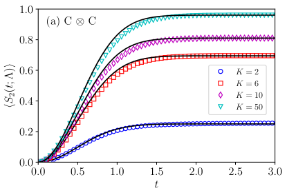
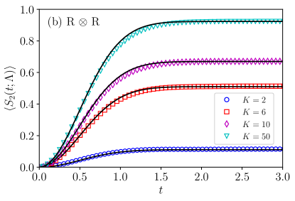
Figure 1: Ensemble averaged linear entropy $\langle S_{2}(t,\Lambda)\rangle$ versus rescaled time for: (a) initial states of C $\otimes$ C type for the RMT transition ensemble defined in Eq. (13), and (b) R $\otimes$ R type. Both use $N_{A}=N_{B}=50$, $\Lambda=10^{-6}$, and various $K$ values. The black solid lines show the corresponding theory of Eq. (41), using Eqs. (43) and (45), respectively.

Ensembles of either the C $\otimes$ C type (coherent random phase) or the R $\otimes$ R type (random superpositions) can be created by defining the appropriate probability densities for the values of the $\{z_{A,j}\}$ and $\{z_{B,k}\}$ in Eq. (35), respectively. For either ensemble, an approximate expression for the ensemble averaged time evolution curve of $S_{2}$ can be derived beginning from Eq. (29). This gives

$$S_{2}(t;\Lambda) \approx c_{A}^{(2)}c_{B}^{(2)}-\sum_{\begin{subarray}{c}j\neq j^{\prime}\\ k\neq k^{\prime}\end{subarray}}|z_{A,j}|^{2}|z_{A,j^{\prime}}|^{2}|z_{B,k}|^{2}|z_{B,k^{\prime}}|^{2}$$

$$\quad\times\exp(\frac{\text{i}\,t}{\sqrt{\Lambda}}[s_{jk,j^{\prime}k}(\Lambda)+s_{j^{\prime}k^{\prime},jk^{\prime}}(\Lambda)]),$$ (39)

where only the first order (in $\epsilon$) correction to the quasi-eigenenergies is to be included. The second-order correction to the quasi-eigenenergies is due to the rotation of eigenstates and are omitted in this regime. After ensemble averaging, $S_{2}$ is given by

$$\langle S_{2}(t;\Lambda)\rangle \approx\langle c_{A}^{(2)}\rangle\langle c_{B}^{(2)}\rangle\big{[}1-\big{\langle}\exp(2\,\text{i}\,t\,x)\big{\rangle}\big{]},$$ (40)

where $x=x_{jk}-x_{j^{\prime}k}+x_{j^{\prime}k^{\prime}}-x_{jk^{\prime}}$ is a sum of four (rescaled) diagonal matrix elements, which behaves like a zero-centered Gaussian random variable of unit variance (shown using Eq. (23)) giving $\langle\exp(2\,\text{i}\,t\,x)\rangle=\exp(-2\,t^{2})$. Thus, the C $\otimes$ C type or R $\otimes$ R type ensemble-averaged $S_{2}$ follows the very simple behavior given by

$$\langle S_{2}(t;\Lambda)\rangle\approx\langle c_{A}^{(2)}\rangle\langle c_{B}^{(2)}\rangle\big{[}1-\exp(-2\,t^{2})\big{]}\ .$$ (41)

Surprisingly, the initial entanglement generation is quadratic in time as opposed to the generally expected linear increase [19, 20, 21, 22, 23, 24], and this is linked to the full system eigenstates retaining their product nature in this regime. Note that if either $K_{A}=1$ or $K_{B}=1$, the coherence measure vanishes and it is necessary to calculate the $\Lambda$ dependent functional form following [18].

Consider C $\otimes$ C type initial states of the form of Eq. (35) where all $|z_{A,j}|=1/\sqrt{K_{A}}$ with random, independently chosen phases, and likewise for subsystem $B$, i.e.

$$\ket{\alpha(0)}=\ket{\alpha_{K_{A}}}_{\text{C}}\otimes\ket{\alpha_{K_{B}}}_{\text{C}}$$ (42)

where $\ket{\alpha_{K}}_{\text{C}}$ is of the form Eq. (4). The long time limiting evolution for a C $\otimes$ C initial state is statistically equivalent to an entangled random phase state with equal intensities. For $K=K_{A}=K_{B}$, the singular values and various entropies of entangled random phase states are studied in [59]. For these initial states, the ensemble average of the coherence measure is same as the individual coherence measures (no fluctuations in coherence measures within the ensemble), and is given by

$$\langle\overline{S}_{2}\rangle=\langle c^{(2)}_{A}\rangle\langle c^{(2)}_{B}\rangle=\left(1-\frac{1}{K_{A}}\right)\left(1-\frac{1}{K_{B}}\right).$$ (43)

The ensemble averaged time evolution of $S_{2}(t;\Lambda)$ for C $\otimes$ C type initial states is shown in Fig. 1 (a) for $K=2,\,,6,\,10,\,50$ compared with the combined results of Eq. (41) and Eq. (43). The agreement is quite good considering that there should be finite $N_{A},\,N_{B}$ and $\Lambda>0^{+}$ corrections. All the necessary details about the numerical calculations shown in Fig. 1 and the other figures are provided in App. B. For $K_{A},K_{B}$ comparable to the respective subsystem dimensionality, i.e. initial states that are tensor product of (nearly) maximally coherent states of the subsystems, the system time evolution generates entanglement $\langle\overline{S}_{2}\rangle\approx 1-1/N_{A}-1/N_{B}$. This is close to the well-known result derived in [34], shown in Eq. (53) ahead. Given that the eigenstates are not thermal and have the product structure, this is a remarkable result in the sense that for an arbitrarily small interaction between the subsystems, a near-maximal entanglement is achieved after a long time by the virtue of maximal coherence in the initial product state.

Next consider R $\otimes$ R type initial product states of the form of Eq. (35), where the $\{z_{A,j}\}$ and $\{z_{B,k}\}$ are random Haar measure complex coefficients where the only constraint is the unit normalization, i.e.

$$\ket{\alpha(0)}=\ket{\alpha_{K_{A}}}_{\text{R}}\otimes\ket{\alpha_{K_{B}}}_{\text{R}}\ .$$ (44)

The ket $\ket{\alpha_{K_{A}}}_{\text{R}}$ is a random pure state in a given subspace of subsystem $A$ Hilbert space spanned by $\mathbb{B}^{\prime}_{A}$ (R type) and similarly for $B$. Performing initial state ensemble averaging of the coherence measure of subsystems, the equilibrium $S_{2}$ value can be computed as

$$\langle\overline{S}_{2}\rangle=\langle c_{A}^{(2)}\rangle\langle c_{B}^{(2)}\rangle=\Big{(}\frac{K_{A}-1}{K_{A}+1}\Big{)}\Big{(}\frac{K_{B}-1}{K_{B}+1}\Big{)},$$ (45)

where the Haar measure average $\langle|z_{A,j}|^{4}\rangle=2/K_{A}(K_{A}+1)$ is used to calculate the above equilibrium value. Figure 1 (b) shows the ensemble averaged $S_{2}(t;\Lambda)$ for R $\otimes$ R type initial states, and an excellent agreement between the theory and numerics is found. For large $K_{A},\,K_{B}$ close to subsystem dimensionality, the equilibrium value is given by $\langle\overline{S}_{2}\rangle\approx 1-2/N_{A}-2/N_{B}$ which is slightly less than that of the C $\otimes$ C type initial states. This can be attributed to the fluctuations in the intensities in the initial states, and is discussed ahead.

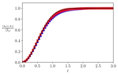
Figure 2: Ensemble averaged linear entropy $\langle S_{2}(t,\Lambda)\rangle$ divided by $\langle\overline{S}_{2}\rangle$. Curves are shown for the RMT transition ensemble of Eq. (13) with $N_{A}=N_{B}=50$, $\Lambda=10^{-6}$, and for various $K$ values. Both C $\otimes$ C type (blue markers) and R $\otimes$ R type (red markers) initial states are indicated. The black solid line shows corresponding theory curve based on Eq. (41).

Remarkably, dividing Eq. (41) by the equilibrium value $\langle\overline{S}_{2}\rangle$ makes all (ensemble-averaged) entanglement production curves for both C $\otimes$ C and R $\otimes$ R types and various $K_{A}$ and $K_{B}$ fall on to one universal curve as illustrated in Fig. 2. It must be emphasized that for obtaining this universal behavior it is crucial to use the rescaled time given by Eq. (27).

IV.1.2 Equilibrium and relaxation

The nature of the equilibrium onto which the system eventually settles can be investigated by examining the variations of $S_{2}$ in time and across the ensemble. As discussed in Sect. II.1, two different useful fluctuation measures are given by $\sigma^{2}(\overline{S}_{2})$ (equilibrium measure) and $\overline{\sigma^{2}(S_{2})}$ (relaxation measure). An equilibrium can be inferred from the former measure if a majority of the initial states evolve to an equilibrium value $\langle\overline{S}_{2}\rangle$ to within small or negligible residual fluctuations. In the $\Lambda\rightarrow 0^{+}$ regime, the equilibrium measure $\sigma^{2}(\overline{S}_{2})$ defined in Eq. (2), can be calculated via Eqs. (38) and (37) in a straightforward way for various initial state ensembles. The relaxation measure $\overline{\sigma^{2}(S_{2})}$ defined in Eq. (3) can be calculated using Eq. (39) in $S^{2}_{2}(t;\Lambda)$ followed by finding its infinite-time average. This gives

$$\overline{\langle S^{2}_{2}(t;\Lambda)\rangle}=\langle(c_{A}^{(2)})^{2}\rangle\langle(c_{B}^{(2)})^{2}\rangle+2\langle c_{A}^{(4)}\rangle\langle c_{B}^{(4)}\rangle,$$ (46)

where a higher order coherence measure $c_{A}^{(4)}$ is introduced based on the $l_{4}$-norm [16] and is defined as

$$c_{A}^{(4)}=\sum_{j\neq j^{\prime}}|z_{A,j}|^{4}|z_{A,j^{\prime}}|^{4},$$ (47)

and similarly for subsystem $B$. The relaxation measure can then be written as

$$\overline{\sigma^{2}(S_{2})}=\sigma^{2}(\overline{S}_{2})+2\frac{\langle c_{A}^{(4)}\rangle\langle c_{B}^{(4)}\rangle}{\langle c_{A}^{(2)}\rangle^{2}\langle c_{B}^{(2)}\rangle^{2}}.$$ (48)

It must be emphasized that fluctuation measures derived here for the $\Lambda\rightarrow 0^{+}$ regime are not valid for initial states either of whose subsystem coherence measures are vanishing. Such cases need special treatment due to the rotation of eigenstates, regardless of how infinitesimal $\Lambda$ is, and are discussed in the next section. It is worth mentioning that for initial unperturbed eigenstates, the $\overline{S}_{2}$ probability density behaves similarly to heavy-tailed type densities spanning $\overline{S}_{2}$ values from $\mathcal{O}(\Lambda)$ to $\mathcal{O}(1)$ [18].

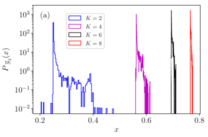
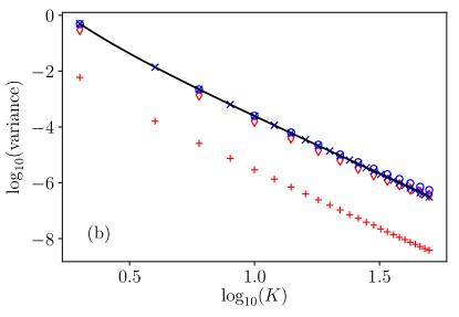
Figure 3: (a) Probability density of $\overline{S}_{2}$ values, and (b) the two fluctuation measures, $\overline{\sigma^{2}\left(S_{2}\right)}$ and $\sigma^{2}\left(\overline{S}_{2}\right)$ for C $\otimes$ C type initial states. Various $K$ values are shown for $N_{A}=N_{B}=50$. In (a) $\Lambda=10^{-6}$. In (b) the black solid line is from Eq. (49) for $\overline{\sigma^{2}\left(S_{2}\right)}$. Compare this prediction to calculated $\overline{\sigma^{2}\left(S_{2}\right)}$ values for $\Lambda=10^{-8}$ ($\color[rgb]{0,0,1}{\times}$) and $\Lambda=10^{-6}$ ($\color[rgb]{0,0,1}{\Circle}$). In addition, calculated values for $\sigma^{2}(\overline{S}_{2})$ (which should lie below $\overline{\sigma^{2}\left(S_{2}\right)}$ ) are plotted for $\Lambda=10^{-8}$ ($\color[rgb]{1,0,0}{+}$) and $\Lambda=10^{-6}$ ($\color[rgb]{1,0,0}{\diamondsuit}$) to illustrate its $\Lambda$-dependence.

The $\overline{S}_{2}$ probability density for C $\otimes$ C type initial states is shown in Fig. 3 (a) for various $K$ values. It is evident from Fig. 3 that for $K=2$ the density is broad and reminiscent of the heavy-tailed nature of the $\overline{S}_{2}$ probability density of E $\otimes$ E type initial state ensemble discussed in the section ahead. As $K$ increases, more unperturbed eigenstates participate resulting in an increasingly sharper $\overline{S}_{2}$ density.

Now consider the two fluctuation measures, $\overline{\sigma^{2}\left(S_{2}\right)}$ and $\sigma^{2}(\overline{S}_{2})$ for C $\otimes$ C type initial states. The relaxation measure can be calculated via Eq. (48) giving

$$\overline{\sigma^{2}(S_{2})}=\frac{2}{K_{A}(K_{A}-1)K_{B}(K_{B}-1)}\sim\frac{2}{K_{A}^{2}K_{B}^{2}},$$ (49)

where the last expression above is valid for large $K_{A}$ and $K_{B}$. Excellent agreement is found between the theory and numerical calculations as illustrated in Fig. 3 (b). This shows that C $\otimes$ C type initial states evolve to an equilibrium state in the strong sense as $K$ increases. Also in Fig. 3 (b) is the comparison of $\sigma^{2}(\overline{S}_{2})$ for $\Lambda=10^{-8}$ and $10^{-6}$, which illustrates its $\Lambda$-dependent nature and that they lie below $\overline{\sigma^{2}(S_{2})}$. It turns out that the leading term of $\sigma^{2}(\overline{S}_{2})$ vanishes for this ensemble, and the effect of eigenstate rotation cannot be neglected for small $K$, leading to this $\Lambda$-dependent behavior.

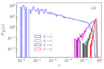
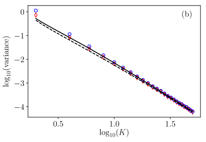
Figure 4: (a) Probability density of $\overline{S}_{2}$ values, and (b) the two fluctuation measures, $\sigma^{2}\left(\overline{S}_{2}\right)$ and $\overline{\sigma^{2}\left(S_{2}\right)}$ for R $\otimes$ R type initial states. Various $K$ values are shown for $N_{A}=N_{B}=50$. In (a) and (b) $\Lambda=10^{-6}$ for the calculations. In (b) the solid black line is the theoretical prediction for $\overline{\sigma^{2}\left(S_{2}\right)}$ and the black dashed line is for $\sigma^{2}\left(\overline{S}_{2}\right)$. The $\color[rgb]{0,0,1}{\Circle}$ are the calculated values for $\overline{\sigma^{2}\left(S_{2}\right)}$ and the $\color[rgb]{1,0,0}{\diamondsuit}$ are the values for $\sigma^{2}\left(\overline{S}_{2}\right)$.

For R $\otimes$ R type initial states, the probability density of $\overline{S}_{2}$ is shown for various $K$-values in Fig. 4 (a). Compared to the C $\otimes$ C type densities, the shapes are quite different and the width of the R $\otimes$ R type densities are wider for any given $K$. For $K=2$, the heavy-tail behavior (straight line in a log-log plot) due to the eigenstate rotation is quite prominent. This is not very surprising since the probability density for random states has inverse square root singularities in the region in which one of the two states is the dominant contribution and the other is very small. This leads the $K=2$ case to being much closer to the unperturbed eigenstate case, which does have the heavy tail (discussed in the next section). As the $K$-value increases, the probability densities become more narrow and the fluctuations about the mean are mainly due to the Haar measure probability density of the components $\{z_{A,j}\}$ and $\{z_{B,k}\}$. Using Eq. (38) and various Haar measure moment averages (see App. C), the fluctuation measure can be computed as

$$\sigma^{2}(\overline{S}_{2}) =\frac{4\,[K_{A}^{3}+K_{B}^{3}+4(K_{A}^{2}+K_{B}^{2})+K_{A}+K_{B}-8]}{(K_{A}^{3}+4K_{A}^{2}+K_{A}-6)(K_{B}^{3}+4K_{B}^{2}+K_{B}-6)}$$

$$\sim\frac{4}{K_{A}^{3}}+\frac{4}{K_{B}^{3}},$$ (50)

where the last line is good for large enough $K_{A},\,K_{B}$. Similarly, it can be shown that

$$\langle c_{A}^{(4)}\rangle =\frac{4(K_{A}-1)}{(K_{A}+1)(K_{A}+2)(K_{A}+3)}\sim\frac{4}{K_{A}^{2}},$$ (51)

and along with Eq. (48) an expression for $\overline{\sigma^{2}(S_{2})}$ can be found in a straightforward way. In contrast to the C $\otimes$ C type case, where the two fluctuation measures are significantly different, for R $\otimes$ R type initial states they are identical to leading order in large-$K_{A},\,K_{B}$ and

$$\overline{\sigma^{2}(S_{2})}\approx\sigma^{2}(\overline{S}_{2})\ .$$ (52)

This is shown in Fig. 4 (b) where a good agreement is observed between the theory and numerical values. Thus, both measures are dominated by their variations about the infinite time average, and the temporal fluctuations are lower order in $K$.

For this regime, the equilibrium measure for various initial state ensembles with non-vanishing coherence implies equilibrium, which becomes sharper as the coherence increases. This is consistent with a transition from weak to strong equilibration as the initial state coherence increases. For initial product states with maximal coherence, the entanglement saturates to that of thermalized states, and they exhibit a strong relaxation (strong thermalization), although the non-scaled relaxation time lengthens to infinity as $\Lambda\rightarrow 0$.

IV.2 Strong interaction regime

In this interaction regime, the eigenstates $\{\ket{jk(\Lambda)}\}$ essentially behave just like that of $N_{A}N_{B}$ - dimensional CUE matrices, and the time evolution of the system shows vanishingly small initial state dependence. Using eigenvector statistics of unitary ensembles for the full system space, the limiting behavior of $\langle\overline{S}_{2}\rangle$ can be derived. The complex coefficients $\bra{\alpha(0)}\ket{jk(\Lambda)}$ in this limit behave the same as the eigenvector components of an $N_{A}N_{B}$-dimensional CUE. For $\ket{jk(\Lambda)}=\sum_{j^{\prime}k^{\prime}}z_{jk}\ket{j^{\prime}k^{\prime}}$, the average purity of the eigenstate is given by [34]

$$\langle\mu_{2,jk}\rangle=\frac{N_{A}+N_{B}}{N_{A}N_{B}+1}\approx\frac{1}{N_{A}}+\frac{1}{N_{B}}.$$ (53)

The average cross-term trace of the reduced density matrices in Eq. (33) can be calculated as

$$\tr_{A}(\rho_{A,jk}\rho_{A,j^{\prime}k^{\prime}}) =\big{\langle}\sum_{jk,j^{\prime}k^{\prime}}z_{jk}z_{j^{\prime}k}^{*}z^{\prime}_{j^{\prime}k^{\prime}}z_{jk^{\prime}}^{\prime*}\big{\rangle}$$

$$=\big{\langle}\sum_{j,k,k^{\prime}}|z_{jk}|^{2}|z^{\prime}_{jk^{\prime}}|^{2}\big{\rangle}$$

$$\approx\sum_{j,k,k^{\prime}}\Big{(}\frac{1}{N_{A}N_{B}}\Big{)}^{2}=\frac{1}{N_{A}}$$ (54)

for large $N_{A},\,N_{B}$, and similarly for the subsystem $B$ trace term. Putting all these together, it can be shown that

$$\langle\overline{S}_{2}^{\infty}\rangle=\lim_{\Lambda\rightarrow\infty}\langle\overline{S_{2}(t;\Lambda)}\rangle\sim 1-\frac{1}{N_{A}}-\frac{1}{N_{B}},$$ (55)

as expected. Furthermore, the expression for average linear entropy derived in [18] in the non-perturbative regime for an initial state ensemble of product eigenstates (shown ahead in Eq. (82)) can be used to describe the situation here with an approximation to the function $C(2;t)$ (defined in Eq. (57) and given by Eq. (98)) that appears in the expression. Since the saturation happens quickly in this regime, the small $t$ approximation of $C(2;t)$ shown in Eq. (58) will suffice giving

$$\langle S_{2}(t;\Lambda)\rangle\approx\langle\overline{S}_{2}^{\infty}\rangle\Bigg{[}1-\exp(-\frac{4\,\pi\,t\,\sqrt{\Lambda}}{\langle\overline{S}_{2}^{\infty}\rangle})\Bigg{]}.$$ (56)

This is in good agreement with numerical simulations whose initial states are of R $\otimes$ R type with $K=2,\,50$ as illustrated in Fig. 5 (a). No initial state dependence is seen and it saturates as expected to $\langle\overline{S}_{2}^{\infty}\rangle$. As $\Lambda\rightarrow\infty$, where the transition becomes complete, the time evolution curve approaches a Heavyside step function scaled by $\langle\overline{S}_{2}^{\infty}\rangle$, saturating almost instantly. The expression in Eq. (56), originally derived with a regularized perturbation theory, extends to the non-perturbative regime using an ‘embedding technique’ developed in [14].

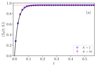
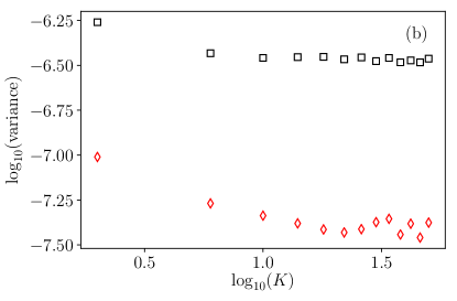
Figure 5: Ensemble averaged linear entropy $\langle S_{2}(t;\Lambda)\rangle$ in (a) and the two variance measures, $\sigma^{2}(\overline{S}_{2})$ and $\overline{\sigma^{2}(S_{2})}$ in (b) for R $\otimes$ R type initial states and $\Lambda=10$, $N_{A}=N_{B}=50$. In (a), $K=2,50$ are shown along with theory curve (of product eigenstates) in Eq. (82). The red dotted line shows the saturation value $\langle\overline{S}_{2}^{\infty}\rangle$. In (b), $\sigma^{2}(\overline{S}_{2})$ ($\color[rgb]{1,0,0}{\diamondsuit}$) and $\overline{\sigma^{2}(S_{2})}$ ($\color[rgb]{0,0,0}$) are shown as a function of $K$.

Quite remarkably, the expression agrees with a recent study based on the entangling power of sequentially applied random diagonal nonlocal operators interlaced with random local unitary operations [60]. Note that entangling power $e_{p}(U)$ is defined as the average entanglement (here linear entropy) produced by the action of a nonlocal gate $U$ on product states sampled from the Haar measure on the subspaces. For $U$ sampled from the diagonal ensemble $U_{AB}$ defined in this paper around Eq. (13) with $\epsilon\ll 1$, the entangling power is quite small $e_{p}(U)\ll 1$. For large enough subsystem dimensions (and hence satisfying $\Lambda\gg 1$), Eq. (55) in [60] representing $e_{p}(U)$ averaged over local unitaries is same as Eq. (56) here with the identification $4\pi t\sqrt{\Lambda}=2\pi^{2}\epsilon^{2}n/3$ where $n$ is the actual time. Note that the average of $e_{p}(U)$ over a Haar distribution of $U$ denoted as $\overline{e_{p}}$ in [60] is approximately the same as $\langle\overline{S}_{2}^{\infty}\rangle$. It may be noted that the entangling power approach involves the local unitaries $U_{A}$ and $U_{B}$ to be different at each time step and this leads to a decorrelation that gives rise to the initial linear growth, also evident in Eq. (56) here. Though $U_{A}$ and $U_{B}$ are the same at each time step here in this paper, in the strong interaction regime the memory from previous time steps is essentially washed out justifying this connection to the entangling power approach.

The equilibrium and relaxation measures are negligibly small compared to the mean value $\langle\overline{S}_{2}\rangle$, i.e. $\sigma^{2}(\overline{S}_{2}),\,\overline{\sigma^{2}(S_{2})}\ll 1$, as evident from Fig. 5 (b), and they show a lack of initial state dependence. Thus the initial state coherence does not play any significant role in the entanglement production in this regime and saturates to the thermal value rapidly. Furthermore, as revealed by the fluctuation measures, the system possesses a very sharp equilibrium and thermalizes in the strong sense where almost all the initial states regardless of their coherence relaxes rapidly to the thermal value.

V Weak and intermediate perturbation regimes

V.1 Weak perturbation regime

V.1.1 E $\otimes$ E type initial states

Consider the initial state ensemble of unperturbed eigenstates $\{\ket{jk}\}$. The coherence measures of both the subsystems are vanishing in the respective preferred subsystem eigenbasis. As mentioned earlier, the entanglement produced for this type of initial states is entirely due to the rotation of eigenstates instigated by the interaction. For sufficiently weak $\Lambda$, the leading order effects arise from the rotation of the initial state $\ket{jk}$ with its energetically nearest neighbor. Since the unperturbed spectrum is a direct product of two independent spectra, the level statistics are Poissonian [17]. There is an absence of level repulsion and two-level near degeneracies are quite frequent. Depending on the interaction strength between the initial state $\ket{jk}$ and its nearest neighbor, the rotation of the pair to perturbed eigenstates can range from little to complete ($\pi/4$ rotation angle).

For an ensemble of eigenstates $\{\ket{jk(\Lambda)}\}$, it was shown in [58] that the linear entropy ranges over the full possible interval $0\leq S_{2}\leq 1/2$. Its probability density displays a heavy-tailed behavior towards large values. In addition, the near degeneracies increased the order of the average eigenstate entanglement from $\mathcal{O}(\Lambda)$ to $\mathcal{O}(\sqrt{\Lambda})$. In [18], it was shown that the mean entanglement production rate increased as

$$\langle S_{2}(t;\Lambda)\rangle\approx C(2;t)\,\sqrt{\Lambda}\,\,,$$ (57)

where $C(2;t)$ is a function of rescaled time and is given in Eq. (98). The short-time behavior of $\langle S_{2}(t;\Lambda)\rangle$ is linear-in-time,

$$\langle S_{2}(t;\Lambda)\rangle\approx 4\,\pi\,t\,\sqrt{\Lambda}\,\,,$$ (58)

and after long time it saturates to

$$\langle\overline{S}_{2}\rangle\approx\frac{5}{8}\,\pi^{3/2}\,\sqrt{\Lambda}\,\,.$$ (59)

In this $\Lambda$ regime, the time evolution of such initial states will remain Schmidt decomposed in the unperturbed eigenstate basis $\mathbb{B}_{AB}$ to $\mathcal{O}(N_{A}^{-1})$ (up to some phase) and is given by

$$\ket{jk(t;\Lambda)}\approx\sum_{l=1}^{N_{A}}\sqrt{\lambda_{l,jk}(t;\Lambda)}\,\ket{(jk)_{l}},$$ (60)

where $\{\ket{(jk)_{l}}\}$ for $l>1$ are unperturbed eigenstates that are energetically close to the initial state $\ket{(jk)_{1}}=\ket{jk}$. The expression for Schmidt eigenvalues $\lambda_{l,jk}(t;\Lambda)$ derived in [18], is given by

$$\lambda_{l,jk}(t;\Lambda) \approx\frac{4\Lambda w_{jk,(jk)_{l}}}{s_{jk,(jk)_{l}}^{2}+4\Lambda w_{jk,(jk)_{l}}}$$

$$\quad\times\sin^{2}\Big{(}\frac{t}{2\sqrt{\Lambda}}\sqrt{s^{2}_{jk,(jk)_{l}}+4\Lambda w_{jk,(jk)_{l}}}\,\Big{)}$$ (61)

for $l>1$ and $\lambda_{1,jk}=1-\sum_{l>1}\lambda_{l,jk}$. This expression is derived using a degenerate perturbation theory where the divergences due to near two-level degeneracies are regularized in a self-consistent manner. The expression for Schmidt eigenvalues in Eq. (61) shows non-self-averaging and oscillatory behavior (quite similar to Rabi oscillations). The linear entropy can be computed using

$$S_{2}(t;\Lambda)\approx 2\sum_{l>1}\Big{(}\lambda_{l,jk}(t;\Lambda)-\lambda_{l,jk}^{2}(t;\Lambda)\Big{)}\,.$$ (62)

The cross terms $\lambda_{l,jk}(t;\Lambda)\lambda_{l^{\prime},jk}(t;\Lambda)$ are neglected in the above since on average they contribute to higher order, $\mathcal{O}(\Lambda)$ [18].

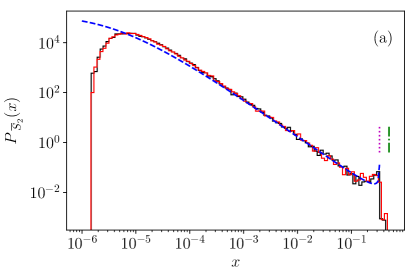
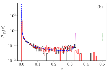
Figure 6: Two views of the $\overline{S}_{2}$ probability density of the E $\otimes$ E type initial state ensemble. In (a) log-log plot illustrating the heavy tail whereas in (b) log-linear which is better for illustrating the endpoint behaviors at $0$ and $1/3$. The blue dashed line shows the theory prediction, Eq. (69). $\Lambda=10^{-6}$ and $N_{A}=N_{B}=50$. The red solid line is the histogram obtained via numerical averaging of individual time evolved curve of initial states after saturation ($t>2$), and the black solid line via Eq. (33). Both sets of data reveal a cutoff around $\mathcal{O}(\Lambda)$. The vertical magenta dotted line and green dot-dashed line shows $x=1/3$ and $1/2$, respectively.

Following the approach in [58], an approximate expression for the probability density of $\overline{S}_{2}$ can be derived in this regime where only the closest unperturbed eigenstate to the initial state $\ket{jk}$ is relevant. In this limit, the infinite time average of Eq. (62) can be calculated as

$$\overline{S}_{2}\approx 4u(1-3u),$$ (63)

where the variable $u$ is given by

$$u=\Big{(}4+\frac{s^{2}}{\Lambda w}\Big{)}^{-1}\,.$$ (64)

The closest neighbor spacing probability density is $P_{\text{CN}}(s)=2\exp(-2s)$ [14] for a Poissonian sequence. The rescaled off-diagonal $\mathcal{V}$-matrix element $w$ has a probability density of an exponential as discussed in Sect. II.5. The probability density of $u$, $P_{u}(x)$, can be calculated from the relation

$$P_{u}(x)=\int_{0}^{\infty}\differential{s}\int_{0}^{\infty}\differential{w}2\text{e}^{-2s}\text{e}^{-w}\delta\Big{(}x-\Big{[}4+\frac{s^{2}}{\Lambda w}\Big{]}^{-1}\Big{)}.$$ (65)

As defined in [58], let

$$f_{\Lambda}(x)=\frac{x}{\Lambda(1-4x)},$$ (66)

then upon carrying out the integral over $w$

$$P_{u}(x)=\int_{0}^{\infty}\differential{s}\,\exp(-2s-s^{2}f_{\Lambda}(x))\Big{[}\frac{2s^{2}}{\Lambda(1-4x)^{2}}\Big{]},$$ (67)

which is similar to Eq. (84) in [58] with appropriate variable transformations. From Eq. (63), $u$ can be written in terms of $x=\overline{S}_{2}$ as

$$u=\frac{1}{6}\Big{(}1-\sqrt{1-3x}\Big{)}$$ (68)

and the solution inconsistent with the non-degenerate perturbation theory is discarded. This gives the $\overline{S}_{2}$ probability density as

$$P_{\overline{S}_{2}}(x)=P_{u}\Big{(}\frac{1}{6}\big{(}1-\sqrt{1-3x}\big{)}\Big{)}\Big{|}\derivative{u}{x}\Big{|}.$$ (69)

Figure 6 illustrates $P_{\,\overline{S}_{2}}(x)$ for $\Lambda=10^{-6}$, where a heavy-tail like distribution can be seen with $\overline{S}_{2}$ covering a range of $\mathcal{O}(\Lambda)$ to $\mathcal{O}(1)$. Notice that around $\overline{S}_{2}=1/3$ the local maximum predicted by Eq. (69) appears. However, some slight deviations indicate that the assumption of just two unperturbed eigenstates participating shows some small corrections due to triple degeneracies that can occur with low probability.

For this ensemble of initial states, a broad distribution of $\overline{S}_{2}$ suggests that equilibrium is not really achieved due to the heavy-tail-like behavior. In addition, due to a dearth of unperturbed eigenstates participating in the time evolved state, a relaxation is not possible. As a result, a large ensemble of initial states are necessary for convergence to the average entanglement production curve.

V.1.2 E $\otimes$ C and E $\otimes$ R type initial states

Consider an initial product state whose one of the subsystem coherence measures is zero in the preferred basis and the other is non-zero

$$\ket{\alpha(0)}=\ket{j}\otimes\Big{(}\sum_{\ket{k}\in\mathbb{B}^{\prime}_{B}}z_{B,k}\ket{k}\Big{)},$$ (70)

where without loss of generality $c_{A}^{(2)}$ is taken to be vanishing. For $K_{B}\ll N_{B}$ an expression for the linear entropy can be derived as follows. The time evolution of the above state using the Schmidt decomposition in Eq. (60) is given by

$$\ket{\alpha(t;\Lambda)}=\sum_{k}\sum_{l}\sqrt{\lambda_{l,jk}(t;\Lambda)}\,\ket{(jk)_{l}},$$ (71)

where any phase factor that may appear is absorbed into $\ket{(jk)_{l}}$. The reduced density matrix constructed out of this time evolved state reads as

$$\rho_{A}(t;\Lambda) =\sum_{k,k^{\prime}}\sum_{l,l^{\prime}}z_{B,k}z_{B,k^{\prime}}^{*}\sqrt{\lambda_{l,jk}(t;\Lambda)\lambda_{l^{\prime},jk^{\prime}}(t;\Lambda)}$$

$$\quad\times\tr_{B}(\ket{(jk)_{l}}\bra{(jk^{\prime})_{l^{\prime}}}).$$ (72)

Note that the set of states $\{\ket{(jk)_{l}}\}$ must be energetically close to the level corresponding to the index pair $(j,k)$ as mentioned earlier, which amounts to having small energy differences between them. Let $(j_{l},k_{l})$ be the index pair of the ket $\ket{(jk)_{l}}$, then for chaotic bipartite Floquet systems considered here the index pair satisfies

$$j_{l}+k_{l}\approx j+k$$ (73)

for $N_{A}\approx N_{B}$ by the virtue of having approximately the same uniform mean level spacing for both the subsystems. This translates to the index pair having a structure $(j_{l},k_{l})=(j\pm l,k\mp l)$ for $l=1,2,3,\ldots$ where $l$ runs up to $N_{A}/2$ typically and energy differences $\theta_{j_{l}k_{l}}-\theta_{jk}$ are approximately $2\pi/N_{A}N_{B}$ on average [58]. Furthermore, for very small perturbations it is enough to keep first and second largest Schmidt eigenvalues in Eq. (60) and neglect the rest [18]. This corresponds to only including the closest neighbor, $\ket{(jk)_{2}}$, of $\ket{jk}$, and the rest are insignificant. However, this argument breaks down when triple degeneracies occur in the unperturbed spectrum. Statistically speaking, this is of very low probability and contributes to higher order than $\mathcal{O}(\sqrt{\Lambda})$. Based on these arguments, the partial trace that appears in Eq. (72) can be computed as follows. For $k=k^{\prime}$ and $l=l^{\prime}$ the partial trace term is $\ket{j_{l}}\bra{j_{l}}$, and that for $k=k^{\prime}$ and $l\neq l^{\prime}$ it vanishes since $k_{l}=k_{l^{\prime}}$ is forbidden according to Eq. (73). In the $k\neq k^{\prime}$ case, the energy difference between levels $(j,k)$ and $(j,k^{\prime})$ is roughly $2\pi/N_{B}$, and so the probability that the set $\{\ket{(jk)_{l}}\}$ and $\{\ket{(jk^{\prime})_{l}}\}$ share a common unperturbed eigenstate or more whose product $\lambda_{l,jk}\lambda_{l^{\prime},jk^{\prime}}$ is also significant is quite small for $K_{B}\ll N_{B}$. Hence, these contributions can be neglected. As $K_{B}$ increases, eventually this argument breaks down.

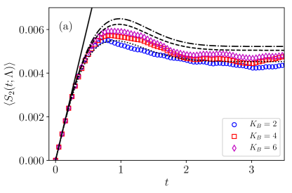
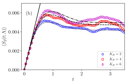
Figure 7: Ensemble averaged linear entropy $\langle S_{2}(t;\Lambda)\rangle$ for Eq. (70)-type initial states versus $t$ for the RMT transition ensemble of Eq. (13) (a) E $\otimes$ C and (b) E $\otimes$ R-type. Both use $N_{A}=N_{B}=50$ and $\Lambda=10^{-6}$. The theory prediction is given by Eq. (77) in black lines, $K=2$ (dotted), $4$ (dashed), $6$ (dot-dashed), and short time behavior Eq. (78) in a black solid line.

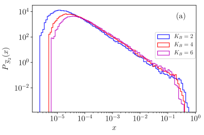
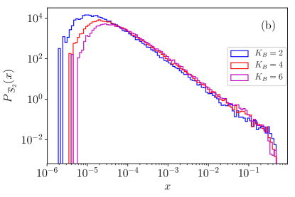
Figure 8: Probability density of $\overline{S}_{2}$ values for initial state type Eq. (70) (a) E $\otimes$ C and (b) E $\otimes$ R type. Various $K_{B}$ values are shown for $N_{A}=N_{B}=50$ and $\Lambda=10^{-6}$.

Putting all this together, it can be shown that the reduced density matrix in Eq. (72) is approximately diagonal in the $\mathbb{B}_{A}$ basis, and the largest Schmidt eigenvalue of $\rho_{A}(t;\Lambda)$ in Eq. (72) is

$$\lambda_{1}(t;\Lambda)\approx\sum_{k}|z_{B,k}|^{2}\lambda_{1,jk}(t;\Lambda),$$ (74)

and rest of the (relevant) Schmidt eigenvalues are

$$\lambda_{l}(t;\Lambda)=|z_{B,k}|^{2}\lambda_{2,jk}(t;\Lambda),$$ (75)

where for each $l=2,\ldots,K_{B}+1$ there is a corresponding pair $(j,k)$ in $\{\lambda_{2,jk}(t;\Lambda)\}_{k=1,\ldots,K_{B}}$, however the ordering is a priori unknown. This gives the linear entropy as

$$S_{2}(t;\Lambda) \approx 2\sum_{k}|z_{B,k}|^{2}\lambda_{2,jk}(t;\Lambda)-2\sum_{k}|z_{B,k}|^{4}\lambda_{2,jk}^{2}(t;\Lambda),$$ (76)

where $\lambda_{1,jk}(t;\Lambda)\approx 1-\lambda_{2,jk}(t;\Lambda)$ is used, and the cross-terms $\lambda_{2,jk}(t;\Lambda)\lambda_{2,jk^{\prime}}(t;\Lambda)$ for $k\neq k^{\prime}$ are neglected since they contribute to $\mathcal{O}(\Lambda)$ on average. Upon ensemble averaging and rearranging

$$\langle S_{2}(t;\Lambda)\rangle\approx\big{[}C(2;t)+2\langle c_{B}^{(2)}\rangle C_{2}(2;t)\big{]}\sqrt{\Lambda},$$ (77)

where the result $\langle\lambda_{2,jk}^{2}\rangle\approx C_{2}(2;t)\sqrt{\Lambda}$ from [18] is used; $C_{2}(2;t)$ is defined in App. D. Expanding the averaged linear entropy for short-time gives

$$\langle S_{2}(t;\Lambda)\rangle=4\pi t\sqrt{\Lambda}+\mathcal{O}(t^{3}),$$ (78)

which is same as that of E $\otimes$ E type initial states. The average linear entropy after long time saturates to

$$\langle\overline{S}_{2}\rangle\approx\Big{(}\frac{5+3\langle c_{B}^{(2)}\rangle}{8}\Big{)}\sqrt{\Lambda}\,\,,$$ (79)

which is obtained by taking $t\rightarrow\infty$ limit of Eq. (77).

Relatively good agreement between the theory prediction and numerical data is found as illustrated in Fig. 7 where C-type ($\ket{\alpha_{K_{B}}}_{\text{C}}$, in (a)) and R-type ($\ket{\alpha_{K_{B}}}_{\text{R}}$, in (b)) states are considered for subsystem $B$ initial states. The deviations from the theory curve that are seen in the plot can be understood by examining the probability density of $\overline{S}_{2}$ as shown in Fig. 8. A broad heavy-tail-like behavior similar to that of E $\otimes$ E initial states is found. Thus, for this type of initial states, equilibrium is a questionable notion. This shows that the convergence to the averaged linear entropy curve of Fig. 7 is quite slow and requires a large sample size. Furthermore, relaxation is not occurring and no self-averaging is apparent. Hence no equilibration occurs even though one of the subsystems has non-vanishing coherence.

V.1.3 C $\otimes$ C and R $\otimes$ R type initial states

Consider the initial states of the form Eq. (35) whose participant unperturbed eigenstates are from the subset $\mathbb{B}_{AB}^{\prime}=\mathbb{B}_{A}^{\prime}\otimes\mathbb{B}_{B}^{\prime}$. As discussed earlier, for the $\Lambda\rightarrow 0^{+}$ regime the time evolved state after a long time remains largely within the subspace described by $\mathbb{B}_{AB}^{\prime}$ of the full Hilbert space. This scenario gets modified as the interaction strength increases where the rotation of eigenstates becomes increasingly relevant. However, for sufficiently small interaction strengths, a perturbed eigenstate $\ket{jk(\Lambda)}$ consists of just $\ket{jk}$ and its energetically closest neighbor $\ket{(jk)_{2}}$, similar to the earlier assumption used for time evolved state $\ket{jk(t;\Lambda)}$. Thus for each $\ket{jk}$ in the subset $\mathbb{B}_{AB}^{\prime}$, there is a corresponding set of such closest neighbors $\{\ket{(jk)_{2}}\}$. The set $\{\ket{(jk)_{2}}\}$ can be divided into two subsets, where one of the subsets has eigenkets outside of $\mathbb{B}_{AB}^{\prime}$ and the other contains the eigenkets that are also in $\mathbb{B}_{AB}^{\prime}$. The elements in these subsets are a priori unknown. This situation brings some non-trivial effects on the entanglement produced and its fluctuation about the equilibrium value $\langle\overline{S}_{2}\rangle$ compared to $\Lambda\rightarrow 0^{+}$ regime and is discussed ahead.

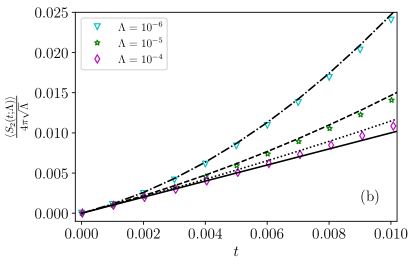
Figure 9: Short time behavior of ensemble averaged $\langle S_{2}(t;\Lambda)\rangle$ for R $\otimes$ R type initial states for $N_{A}=N_{B}=50$. In (a) $\Lambda=10^{-6}$ with various $K$ values. The black solid line represents Eq. (58), and other black lines indicate the combined theory in Eq. (80) corresponding to various $K$ values. In (b) $K=50$ with the $\Lambda$ values indicated in the legend. The black solid line represents Eq. (58) and the other black lines correspond to various $\Lambda$ values of the combined theory given in Eq. (80). All the curves are scaled by $4\pi\sqrt{\Lambda}$.

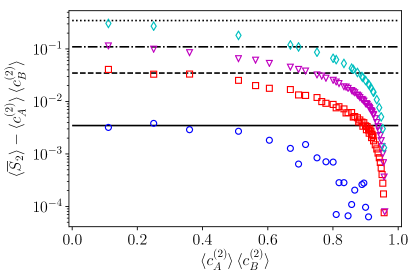
Figure 10: The difference of $\langle\overline{S}_{2}\rangle$ and initial state coherence $\langle c_{A}^{(2)}\rangle\langle c_{B}^{(2)}\rangle$ as a function of the initial state coherence for various interaction strengths $\Lambda=10^{-6}$ ($\color[rgb]{0,0,1}{\Circle}$), $10^{-4}$ ($\color[rgb]{1,0,0}{\square}$), $10^{-3}$ ($\color[rgb]{1,0,1}$), $10^{-2}$ ($\color[rgb]{0,1,1}$) are shown where dimensionality $N_{A}=N_{B}=50$. The horizontal black lines show Eq. (59) for various $\Lambda$ where the solid line corresponds $\Lambda=10^{-6}$ and dotted line is for $\Lambda=10^{-2}$.

Numerical data reveal that the effect of eigenstate rotation is quite evident during the initial entanglement production phase. For any $\Lambda>0^{+}$, a linear-in-time growth is found, which happens to be the same as that of E $\otimes$ E initial states given in Eq. (58) for $t\approx 0$. The theory derived for $\Lambda\rightarrow 0^{+}$ in Eq. (38) fails for this initial entanglement growth phase and after including the correction due to the rotation of eigenstates, the entanglement production for short times is given by

$$\langle S_{2}(t;\Lambda)\rangle\approx 4\pi t\sqrt{\Lambda}+2\langle c_{A}^{(2)}\rangle\langle c_{B}^{(2)}\rangle t^{2}\ ,$$ (80)

which quantifies a competition between quadratic entanglement growth and the generally expected linear behavior. Depending on the circumstances, the quadratic or linear term may dominate, and the ratio of the terms generates a crossover time scale given by

$$t^{*}=\frac{2\pi\sqrt{\Lambda}}{\langle c_{A}^{(2)}\rangle\langle c_{B}^{(2)}\rangle}$$ (81)

at which the linear and quadratic growth terms contribute equally. For $t\ll t^{*}$ a prominent linear growth is seen and for $t>t^{*}$ it becomes increasingly quadratic. An interesting aspect of the expression for the crossover time scale is that for small enough $\Lambda$ and large enough quantum coherence in the initial state, $t^{*}\rightarrow 0$, the linear regime collapses, and short time entanglement production effectively displays purely quadratic behavior. On the other hand, for values of $\Lambda$ and quantum coherence leading to a $t^{*}$ which is an appreciable fraction of unity (greater than the short scaled time regime), this quadratic regime ceases to exist, and only the linear regime behavior results. Note that quadratic growth has been found to exist in strongly coupled holographic systems [61, 62], where quadratic behavior transitions to a linear growth, and in random local Gaussian circuits [63].

The crossover between linear and quadratic entanglement growth during the initial phase of the time evolution is shown in Fig. 9. In Fig. 9 (a) the average entanglement growth for fixed $\Lambda=10^{-6}$ and initial states of type R $\otimes$ R with various $K$ values are shown (C $\otimes$ C type initial states show similar behavior and are not displayed here), where the crossover time scales $t^{*}=0.056,0.017,0.0068$, for $K=2,4,50$, respectively. For small $K_{A}$ and $K_{B}$ values, the initial states are more like E $\otimes$ E type and they show a prominent linear-in-time behavior for a long period during the initial phase as opposed to the initial states whose $K_{A}\sim N_{A}$ and $K_{B}\sim N_{B}$ where the linear-in-time behavior transitions to a quadratic behavior rather quickly. As the interaction strength increases, a dominant linear-in-time entanglement growth is found stretching to longer and longer times predicted by the time scale $t^{*}$. This is displayed in Fig. 9 (b) where $K=50$ and $\Lambda=10^{-6},10^{-5},10^{-4}$ whose crossover time scales are $t^{*}=0.0068,0.021,0.068$, respectively. Here $\langle S_{2}(t;\Lambda)\rangle$ is scaled by $4\pi\sqrt{\Lambda}$ so that all the curves for various $\Lambda$ have the same slope for easier visual comparison.

The influence of eigenstate rotation can be seen in the difference of $\langle\overline{S}_{2}\rangle$ and $\langle c_{A}^{(2)}\rangle\langle c_{B}^{(2)}\rangle$ for various interaction strengths as shown in Fig. 10. This difference is expected to be of the order $\mathcal{O}(\sqrt{\Lambda})$ based on what is known for the E $\otimes$ E case in Eq. (59), illustrated in the plot as horizontal black lines. As the initial state coherence increases, there are increasing deviations from this expectation due to the corrections that strongly depend on the initial state coherence. For near-maximal initial state coherence, the eigenstate rotation has negligible affect on the saturation value $\langle\overline{S}_{2}\rangle$, and the difference vanishes.

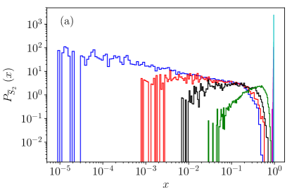
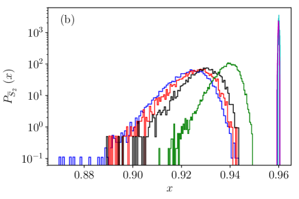
Figure 11: Probability density of $\overline{S}_{2}$ values for R $\otimes$ R type initial states for (a) $K=2$, (b) $K=50$. $\Lambda=10^{-6}$ (blue), $10^{-4}$ (red), $10^{-3}$ (black), $10^{-2}$ (green), $1$ (magenta), $10$ (cyan).

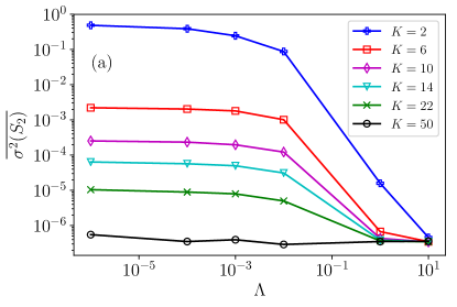
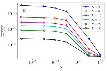
Figure 12: The relaxation measure $\overline{\sigma^{2}(S_{2})}$ as a function of $\Lambda$ for (a) C $\otimes$ C and (b) R $\otimes$ R type initial states. Various $K$ values with $N_{A}=N_{B}=50$.

Furthermore, the probability density of $\overline{S}_{2}$ becomes increasingly localized as the interaction strength increases, which is not surprising. The change in shape is more pronounced for $K_{A}\ll N_{A}$, $K_{B}\ll N_{B}$, where it transitions from the broad heavy-tail like behavior to a localized Gaussian-like probability density around $\Lambda=10^{-2}$ as shown in Fig. 11 (a). On the other hand, for $K_{A}\sim N_{A}$, $K_{B}\sim N_{B}$ the density is a narrow, distorted Gaussian-like shape, which becomes even narrower as the interaction strength is increased; see Fig. 11 (b). This also is not surprising because for small $K_{A},\,K_{B}$ and $\Lambda\rightarrow 0^{+}$ the probability density is broad whereas for large $K_{A},\,K_{B}$ it is quite localized as seen in Figs. 3 (a), 4 (a). So as the interaction strength increases, for initial states with small $K_{A},\,K_{B}$ more and more unperturbed eigenstates are perturbatively added leading to a more localized Gaussian-like distribution by the virtue of central limit theorem along with self-canceling of terms involving oscillating eigencomponents with random frequencies that appear in the $\overline{S}_{2}$ expression. This also means that as the interaction strength increases, more and more initial states relax to the equilibrium as observed in Figs. 12 (a) and (b) where both C $\otimes$ C and R $\otimes$ R type initial states are shown, respectively. As the interaction strength increases, a significant change in $\overline{\sigma^{2}(S_{2})}$ occurs only for $K=2$. Although, for most $K$, a drop occurs across the intermediate strength perturbation regime. Interestingly, for maximally coherent C $\otimes$ C type initial states ($K=50$), the relaxation measure is nearly constant and much less than unity, even extending to the intermediate and strong regimes, implying that the system attains thermal equilibrium eventually. Note that the time taken to reach saturation gets shorter and shorter as $\Lambda$ increases. In other words, the maximal coherence in the initial product states is an alternate path to thermalization of the system under time evolution with $\Lambda$ determining how rapidly it reaches thermal equilibrium regardless of whether the eigenstates of the system are thermal or not.

V.2 Intermediate perturbation regime

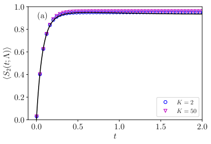
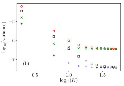
Figure 13: (a) Ensemble averaged linear entropy $\langle S_{2}(t;\Lambda)\rangle$ as a function of rescaled time $t$ is shown for $K=2,\,50$ R $\otimes$ R type initial states. The black solid curve shows the E $\otimes$ E type result in Eq. (82) for the non-perturbative regime. (b) The two fluctuation measures, $\sigma^{2}(\overline{S}_{2})$ and $\overline{\sigma^{2}(S_{2})}$ for C $\otimes$ C ($\color[rgb]{0,0,1}{+}$ and $\color[rgb]{0,1,0}$, respectively) and R $\otimes$ R type ($\color[rgb]{0,0,0}$ and $\color[rgb]{1,0,0}{\Circle}$, respectively). For both (a) and (b) $N_{A}=N_{B}=50$ and $\Lambda=1$.

This regime can be viewed as an interpolation or transition from the weak to strong interaction regime, where a weak dependence on the initial state coherence is observed which vanishes as the interaction strength increases. From this observation, the expression for $\langle S_{2}(t;\Lambda)\rangle$ derived in the study [18] for E $\otimes$ E initial states in the non-perturbative regime

$$\langle S_{2}(t;\Lambda)\rangle\approx\langle\overline{S}_{2}^{\infty}\rangle\Bigg{[}1-\exp(-\frac{C(2;t)\sqrt{\Lambda}}{\langle\overline{S}_{2}^{\infty}\rangle})\Bigg{]},$$ (82)

can be used as a decent approximation to the entanglement produced for any initial product states. This is illustrated in Fig. 13 (a) for $\Lambda=1$. The saturation values for $K=2,\,50$ can be seen to be slightly higher than that the theory curve in Eq. (82) and $K=50$ curve saturates above that of $K=2$. Note that in the strong interaction regime discussed previously in Sect. IV.2 the above equation was used to show that the average entanglement generated is largely independent of the initial (product) state.

The probability density of $\overline{S}_{2}$ for $\Lambda=1$ is highly localized in contrast to the ones in the weak perturbative regime; see Fig. 11. The initial state coherence appears to play a role in the width of the density. The $K=50$ case is almost identical to that of $\Lambda=10$ in the strong interaction regime. Furthermore, the fluctuation measures obtained numerically for C $\otimes$ C and R $\otimes$ R type initial state ensembles show that a majority of the initial states eventually attain the equilibrium value $\langle\overline{S}_{2}\rangle$ and remain there as shown in Fig. 13 (b).

V.3 Discussion

It is worthwhile to collect all the results discussed so far to get an overall picture of how relaxation and equilibration depend on the quantum coherence in an initial product state and the interaction strength between the subsystems. Together, the coherence and transition parameter govern the entanglement growth and its saturation to an equilibrium (if it exists) and the nature of the equilibration.

In the ultra-weak interaction regime, where the rotation of eigenstates are neglected, an existence of equilibrium can be established based on the equilibrium measure where the equilibrium becomes sharper as the average coherence in the initial state ensemble increases. The coherence of the initial states also affects its ability to equilibrate. A weak to strong equilibration is found to occur as the average coherence of the initial state ensemble increases. In particular, for maximally coherent initial product states the system thermalizes after sufficiently long time and remains thermalized for almost all the initial states as indicated by negligibly small fluctuations about the equilibrium. Furthermore, a quadratic initial entanglement growth is seen in this regime characterized by the average coherence of the ensemble under consideration.

A similar story can be said for weak interaction regime, except for the new effects that arise due to the rotation of eigenstates. Firstly, for initial states whose coherence is vanishing an equilibrium is questionable and hence no relaxation can be seen. The initial entanglement growth is linear-in-time and is purely due to the rotation of eigenstates and the rate is dictated by the transition parameter. The average entanglement saturation value is perturbative and is also dictated strongly by the transition parameter. Secondly, for initial state ensembles with non-vanishing average coherence, a competition between linear and quadratic growths occurs in the initial phase. While the linear-in-time behavior is same for any kind of initial state ensemble, the quadratic growth depends strongly on the average coherence. Furthermore, the entanglement saturation shows strong dependence on the transition parameter for initial state ensembles with low average coherence while a weak dependence is seen for ensembles with high coherence.

For intermediate and strong interaction regimes, little to negligibly small dependence on the initial states is observed, including the ones with vanishing coherence. In these regimes, a strong equilibration is seen. A noteworthy point here is that the initial state ensemble with maximal coherence thermalizes regardless of the strength of the interaction but how rapidly it thermalizes is controlled by the transition parameter. Larger the transition parameter, shorter it takes to thermalize. Table LABEL:tab:table summarizes the key results.

Table 1: Various initial state ensembles and nature of the equilibrium and initial entanglement growth in various interaction regimes.

Initial state ensemble	Interaction regime
	Ultra-weak	Weak	Intermediate	Strong
E $\otimes$ E, E $\otimes$ C, E $\otimes$ R	no equilibration,	no equilibration,	strong equilibration,	strong thermalization,
(vanishing coherence)	initial linear growth	initial linear growth	initial linear growth	initial linear growth
C $\otimes$ C, R $\otimes$ R	weak equilibration,	weak equilibration,	strong equilibration,	strong thermalization,
(low coherence)	initial quadratic growth	late linear to quadratic crossover	initial linear growth	initial linear growth
C $\otimes$ C, R $\otimes$ R	strong equilibration,	strong equilibration,	strong equilibration,	strong thermalization,
(high coherence)	initial quadratic growth	early linear to quadratic crossover	initial linear growth	initial linear growth
C $\otimes$ C	strong thermalization	strong thermalization	strong thermalization	strong thermalization
(maximal coherence)	initial quadratic growth	early linear to quadratic crossover	initial linear growth	initial linear growth

VI Summary and outlook

In this paper, some of the direct consequences of quantum coherence towards the entanglement production, equilibration and thermalization are presented. In an earlier study [18], the entanglement production of special E $\otimes$ E type initial states was found to depend only on a universal transition parameter $\Lambda$, and the rescaled time $t$, which as shown in this study, generalizes the scope of these universal quantities to generic initial states. As guided by perturbation theory, various perturbation regimes were identified.

In the ultra-weak regime $\Lambda\rightarrow 0^{+}$ where the diagonal elements of the perturbation matrix are relevant and the effect of rotation of eigenstates is neglected, it was analytically shown that the entanglement production is a Gaussian as a function of time and saturates to the product of coherence measures (a coherence measure based on the $l_{2}$-norm) of the subsystems in their respective preferred eigenstate basis. This implies an unusual initial quadratic time dependent increase in the entanglement. Whether quadratic or linear behavior is to be expected is contained in Eq. (80). It was found that for initial (product) states whose subsystem coherence measures are near maximal after long time the system saturates to the maximal entanglement. Furthermore, such states show thermalization as evident from the distribution of infinite time average of linear entropy and the relaxation measure, which is a remarkable result noting that the interaction between the subsystems is ultra-weak, and the full system eigenstates are barely different from the non-interacting case. This shows that quantum coherence acts as a resource for equilibration and thermalization.

In the weak regime, where the eigenstate rotation is relevant in the perturbation theory, it was found that the probability density of the infinite time linear entropy average of initial states whose product of subsystem coherence measures is vanishing has a broad heavy-tail like behavior and shows no relaxation. Entanglement production is of the order $\mathcal{O}(\sqrt{\Lambda})$ on average and shows a slow convergence to the average due to the heavy-tailed nature of the distribution. In the initial entanglement growth phase, it can be shown that the entanglement production is linear in time and the rate is proportional to $\sqrt{\Lambda}$. This initial linear-in-time entanglement growth is seen regardless of the initial state coherence and is universal, even for large $\Lambda$. The effect of eigenstate rotation is also evident in the entanglement saturation values, especially for initial states whose coherence is close to minimal. On the other hand, initial states with near-maximal coherence are not dependent on this. Lastly, in the intermediate regime and beyond, the entanglement production appears to have little to no dependence on the initial product states and shows an exponential behavior.

In the present study, an RMT transition ensemble was used to mimic a bipartite system whose subsystems are fully quantum chaotic. For a real dynamical system either single-particle or many-body, features like eigenstate scarring [64], $k$-body interactions in case of many-body systems (see the review [43]) and other dynamical features may give rise to some system specific deviations to the universal features presented in this paper. It would be interesting to know how the universal features presented here would change if the subsystems are not fully chaotic, where the notion of the transition parameter may not exist due to selection rules and existence of local integrals of motion (see the review [9]). As seen in this study, the initial product state coherence plays a crucial role in determining the fate of the interacting bipartite system at long times. This study may shed light on understanding the phase transition towards thermalization not just with the interaction strength, but also due to coherence in the initial state. Moreover, it would be interesting to understand the entanglement production in a semiclassical sense similar to the earlier fidelity studies that related the transition parameter to the classical action diffusion coefficient and the phase space volume in the ultra-weak perturbation regime [56, 57].

Appendix A Derivation of variances of $\mathcal{V}$ matrix elements

Starting from Eq. (18), the expression for the variance is

$$\langle|{\cal V}_{jk,j^{\prime}k^{\prime}}|^{2}\rangle =\Big{\langle}\sum_{ab,a^{\prime}b^{\prime}}u_{ja}^{A*}\,u_{kb}^{B*}\,u_{j^{\prime}a}^{A}\,u_{k^{\prime}b}^{B}\,(2\pi\xi_{ab})$$

$$\qquad\times u_{ja^{\prime}}^{A}\,u_{kb}^{B}\,u_{j^{\prime}a}^{A*}\,u_{k^{\prime}b}^{B*}\,(2\pi\xi_{a^{\prime}b^{\prime}})\Big{\rangle}.$$ (83)

Given the probability density of $\xi_{ab}$, Eq. (14), and independence

$$\langle\xi_{ab}\,\xi_{a^{\prime}b^{\prime}}\rangle=\delta_{ab,a^{\prime}b^{\prime}}\frac{1}{12},$$ (84)

the variance reduces to the expression

$$\langle|\mathcal{V}_{jk,j^{\prime}k^{\prime}}|^{2}\rangle=\frac{\pi^{2}}{3}\Big{\langle}\sum_{ab}|u_{ja}^{A}|^{2}\,|u_{j^{\prime}a}^{A}|^{2}\,|u_{kb}^{B}|^{2}\,|u_{k^{\prime}b}^{B}|^{2}\Big{\rangle},$$ (85)

where Haar averaging over unitary groups remains to be performed. Using the known results [53] gives

$$\langle|u_{ja}^{A}|^{2}\,|u_{j^{\prime}a}^{A}|^{2}\rangle=\frac{1+\delta_{jj^{\prime}}}{N_{A}(N_{A}+1)},$$ (86)

and similarly for subsystem $B$ in Eq. (85). Summing over the variables $a,b$ leads to the result in Eq. (19).

The covariance, $\langle x_{jk}\,x_{j^{\prime}k^{\prime}}\rangle$, in Eq. (23) is given by

$$\langle x_{jk}x_{j^{\prime}k^{\prime}}\rangle=\frac{\langle\mathcal{V}_{jk,jk}\,\mathcal{V}_{j^{\prime}k^{\prime},j^{\prime}k^{\prime}}\rangle}{\sqrt{\langle|\mathcal{V}_{jk,jk}|^{2}\rangle}\sqrt{\langle|\mathcal{V}_{j^{\prime}k^{\prime},j^{\prime}k^{\prime}}|^{2}\rangle}},$$ (87)

where making use of $\sqrt{\langle|\mathcal{V}_{jk,jk}|^{2}\rangle}=\sqrt{\langle|\mathcal{V}_{j^{\prime}k^{\prime},j^{\prime}k^{\prime}}|^{2}\rangle}$ and Eq. (19) gives

$$\sqrt{\langle|\mathcal{V}_{jk,jk}|^{2}\rangle}\sqrt{\langle|\mathcal{V}_{j^{\prime}k^{\prime},j^{\prime}k^{\prime}}|^{2}\rangle}=\frac{4\pi^{2}}{3(N_{A}+1)(N_{B}+1)}\,.$$ (88)

That leaves the $\langle\mathcal{V}_{jk,jk}\,\mathcal{V}_{j^{\prime}k^{\prime},j^{\prime}k^{\prime}}\rangle$ computation to be done. Starting from Eq. (18) and using Eq. (84) gives

$$\langle\mathcal{V}_{jk,jk}\,\mathcal{V}_{j^{\prime}k^{\prime},j^{\prime}k^{\prime}}\rangle=\frac{\pi^{2}}{3}\Big{\langle}\sum_{ab}|u_{ja}^{A}|^{2}\,|u_{j^{\prime}a}^{A}|^{2}\,|u_{kb}^{B}|^{2}\,|u_{k^{\prime}b}^{B}|^{2}\Big{\rangle}$$ (89)

and performing Haar averaging on the subsystem unitary groups, as in Eq. (85), establishes Eq. (23).

Appendix B Details of numerical calculations

All the calculations presented in this article are based on realizations of the random matrix transition ensemble defined in Eq. (13) using subsystem dimensionality $N_{A}=N_{B}=50$. The sample size details of time evolution raw data for various C $\otimes$ C and R $\otimes$ R type initial state ensembles and all $\Lambda$ values are shown in Table. 2 as initial state sampled per realization $\times$ total number of realizations.

Table 2: Various $\Lambda$ values and corresponding initial state samples per realization $\times$ number of realizations.

$\Lambda$	C $\otimes$ C	R $\otimes$ R	E $\otimes$ E	E $\otimes$ C	E $\otimes$ R
$10^{-6}$	1250 $\times$ 5	2500 $\times$ 5	2500 $\times$ 20	2500 $\times$ 20	2500 $\times$ 5
$10^{-4}$	1250 $\times$ 5	750 $\times$ 5	N/A	N/A	N/A
$10^{-3}$	750 $\times$ 5	750 $\times$ 5	N/A	N/A	N/A
$10^{-2}$	2500 $\times$ 5	2500 $\times$ 5	N/A	N/A	N/A
$1$	2500 $\times$ 2	2500 $\times$ 2	N/A	N/A	N/A
$10$	50 $\times$ 5	50 $\times$ 5	N/A	N/A	N/A

For the short time behavior depicted in Fig. 9 and for various $\Lambda$ values 1000 $\times$ 5 initial states were used instead. In addition, for Fig. 6 data generated for the $\overline{S}_{2}$ probability density based on the infinite time average expression in Eq. (33) used 2500 $\times$ 10 initial states.

Appendix C Eigenvector statistics of unitary ensemble

Consider an eigenvector $\ket{\alpha}$ of an $N$-dimensional CUE matrix of unitary ensemble. Represented in some fixed basis $\ket{i}$, it is given by $\ket{\alpha}=\sum_{i=1}^{N}z_{i}\ket{i}$, where $z_{i}$ are complex coefficients. The only constraint is the normalization, $\sum_{i}|z_{i}|^{2}=1$. The probability density of the eigenvector components are given by [43, 65, 66]

$$P(z_{1},z_{2},\ldots,z_{N})=\frac{(N-1)!}{\pi^{N}}\delta\Big{(}\sum_{i=1}^{N}|z_{i}|^{2}-1\Big{)},$$ (90)

for which reduced probability density can be found by integrating out $N-l$ variables resulting in

$$P_{l}(z_{1},z_{2},\ldots,z_{l})=\frac{\Gamma(N)}{\pi^{l}\Gamma(N-l)}\Big{(}1-\sum_{i=1}^{l}|z_{i}|^{2}\Big{)}^{N-l-1}.$$ (91)

Using the above reduced probability density various moments of $z_{i}$ can be computed analytically. Below a list of useful moments relevant to the main text are given

$$\langle|z_{i}|^{4}\rangle=\frac{2}{N(N+1)},$$ (92)

$$\langle|z_{i}|^{2}|z_{j}|^{2}\rangle=\frac{1}{N(N+1)}\quad\text{for}\,i\neq j,$$ (93)

$$\langle|z_{i}|^{8}\rangle=\frac{24}{N(N+1)(N+2)(N+3)},$$ (94)

and

$$\langle|z_{i}|^{4}|z_{j}|^{4}\rangle=\frac{4}{N(N+1)(N+2)(N+3)}\quad\text{for}\,i\neq j.$$ (95)

Appendix D $C(2;t)$ and $C_{2}(2;t)$ functions

The $C(2;t)$ and $C_{2}(2;t)$ functions are defined in a previous work [18] for the context of the ensemble averaged unperturbed eigenstate time evolution, Eq. (60). The function $C_{2}(2;t)$ is given by

$$\Big{\langle}\sum_{l>1}\lambda_{l,jk}^{2}(t;\Lambda)\Big{\rangle} =C_{2}(2;t)\sqrt{\Lambda},$$ (96)

where

$$C_{2}(2;t) =\int_{0}^{\infty}\differential{w}\int_{-\infty}^{\infty}\differential{z}\,\Bigg{(}\frac{4z}{z^{2}+4w}\Bigg{)}^{2}\exp(-w)$$

$$\quad\times\sin^{4}\Big{(}\frac{t}{2}\sqrt{z^{2}+4w}\Big{)}.$$ (97)

The function $C(2;t)$ defined in Eq. (57) is given by

$$C(2;t)=\pi t\Big{(}3\text{e}^{-t^{2}}-\frac{1}{2}\text{e}^{-4t^{2}}\Big{)}+\pi^{3/2}\text{erf}(t)\Big{(}\frac{1}{2}+3t^{2}\Big{)}$$

$$\qquad\qquad+\pi^{3/2}\text{erf}(2t)\Big{(}\frac{1}{8}-3t^{2}\Big{)},$$ (98)

where $\text{erf}(x)=(2/\sqrt{\pi})\int_{0}^{x}\text{e}^{-t^{2}}\differential{t}$ is the error function.

References

- [1] M. Rigol, V. Dunjko, and M. Olshanii, Thermalization and its mechanism for generic isolated quantum systems, Nature 452, 854 (2008).
- [2] J. M. Deutsch, Quantum statistical mechanics in a closed system, Phys. Rev. A 43, 2046 (1991).
- [3] M. Srednicki, Chaos and quantum thermalization, Phys. Rev. E 50, 888 (1994).
- [4] L. D’Alessio, Y. Kafri, A. Polkovnikov, and M. Rigol, From quantum chaos and eigenstate thermalization to statistical mechanics and thermodynamics, Adv. Phys. 65, 239 (2016).
- [5] K. He and M. Rigol, Initial-state dependence of the quench dynamics in integrable quantum systems. III. Chaotic states, Phys. Rev. A 87, 043615 (2013).
- [6] E. J. Torres-Herrera and L. F. Santos, Effects of the interplay between initial state and Hamiltonian on the thermalization of isolated quantum many-body systems, Phys. Rev. E 88, 042121 (2013).
- [7] M. Collura, M. Kormos, and P. Calabrese, Stationary entanglement entropies following an interaction quench in 1D Bose gas, J. Stat. Mech. , P01009 (2014).
- [8] M. Rigol and M. Srednicki, Alternatives to eigenstate thermalization, Phys. Rev. Lett. 108, 110601 (2012).
- [9] D. A. Abanin, E. Altman, I. Bloch, and M. Serbyn, Colloquium: Many-body localization, thermalization, and entanglement, Rev. Mod. Phys. 91, 021001 (2019).
- [10] R. Khare and S. Choudhury, Localized dynamics following a quantum quench in a non-integrable system: an example on the sawtooth ladder, J. Phys. B 54, 015301 (2020).
- [11] J. Rau and B. Müller, From reversible quantum microdynamics to irreversible quantum transport, Phys. Rep. 272, 1 (1996).
- [12] J. B. French, V. K. B. Kota, A. Pandey, and S. Tomsovic, Statistical properties of many particle spectra v: fluctuations and symmetries, Ann. Phys. (N.Y.) 181, 198 (1988).
- [13] S. C. L. Srivastava, S. Tomsovic, A. Lakshminarayan, R. Ketzmerick, and A. Bäcker, Universal scaling of spectral fluctuation transitions for interacting chaotic systems, Phys. Rev. Lett. 116, 054101 (2016).
- [14] A. Lakshminarayan, S. C. L. Srivastava, R. Ketzmerick, A. Bäcker, and S. Tomsovic, Entanglement and localization transitions in eigenstates of interacting chaotic systems, Phys. Rev. E 94, 010205(R) (2016).
- [15] Z. Bai and S. Du, Maximally coherent states, Quantum Inf. Comput. 15, 1355 (2015).
- [16] A. Streltsov, G. Adesso, and M. B. Plenio, Colloquium: Quantum coherence as a resource, Rev. Mod. Phys. 89, 041003 (2017).
- [17] T. Tkocz, M. Smaczyński, M. Kus, O. Zeitouni, and K. Życzkowski, Tensor products of random unitary matrices, Random Matrices: Theor. Appl. 1, 1250009 (2012).
- [18] J. J. Pulikkottil, A. Lakshminarayan, S. C. L. Srivastava, A. Bäcker, and S. Tomsovic, Entanglement production by interaction quenches of quantum chaotic subsystems, Phys. Rev. E 101, 032212 (2020).
- [19] W. H. Zurek and J. P. Paz, Decoherence, chaos, and the second law, Phys. Rev. Lett. 72, 2508 (1994).
- [20] P. A. Miller and S. Sarkar, Signatures of chaos in the entanglement of two coupled quantum kicked tops, Phys. Rev. E 60, 1542 (1999).
- [21] D. Monteoliva and J. P. Paz, Decoherence and the rate of entropy production in chaotic quantum systems, Phys. Rev. Lett. 85, 3373 (2000).
- [22] A. Tanaka, H. Fujisaki, and T. Miyadera, Saturation of the production of quantum entanglement between weakly coupled mapping systems in a strongly chaotic region, Phys. Rev. E 66, 045201 (2002).
- [23] H. Fujisaki, T. Miyadera, and A. Tanaka, Dynamical aspects of quantum entanglement for weakly coupled kicked tops, Phys. Rev. E 67, 066201 (2003).
- [24] J. N. Bandyopadhyay and A. Lakshminarayan, Entanglement production in coupled chaotic systems: Case of the kicked tops, Phys. Rev. E 69, 016201 (2004).
- [25] P. Calabrese and J. Cardy, Evolution of entanglement entropy in one-dimensional systems, J. Stat. Mech.: Theory Exp. 2005, P04010 (2005).
- [26] H. Kim and D. A. Huse, Ballistic spreading of entanglement in a diffusive nonintegrable system, Phys. Rev. Lett. 111, 127205 (2013).
- [27] A. M. Kaufman, M. E. Tai, A. Lukin, M. Rispoli, R. Schittko, P. M. Preiss, and M. Greiner, Quantum thermalization through entanglement in an isolated many-body system, Science 353, 794 (2016), eprint https://www.science.org/doi/pdf/10.1126/science.aaf6725.
- [28] M. C. Bañuls, J. I. Cirac, and M. B. Hastings, Strong and weak thermalization of infinite nonintegrable quantum systems, Phys. Rev. Lett. 106, 050405 (2011).
- [29] C.-J. Lin and O. I. Motrunich, Quasiparticle explanation of the weak-thermalization regime under quench in a nonintegrable quantum spin chain, Phys. Rev. A 95, 023621 (2017).
- [30] N. Linden, S. Popescu, A. J. Short, and A. Winter, Quantum mechanical evolution towards thermal equilibrium, Phys. Rev. E 79, 061103 (2009).
- [31] J. M. Deutsch, Eigenstate thermalization hypothesis, Rep. Prog. Phys 81, 082001 (2018).
- [32] M. Srednicki, Thermal fluctuations in quantized chaotic systems, J. Phys. A 29, L75 (1996).
- [33] L. C. Andrews, R. L. Phillips, C. Y. Hopen, and M. A. Al-Habash, Theory of optical scintillation, J. Opt. Soc. Am. A 16, 1417 (1999).
- [34] E. Lubkin, Entropy of an n‐system from its correlation with a k‐reservoir, J. Math. Phys. 19, 1028 (1978).
- [35] J. Aberg, Quantifying Superposition, arXiv e-prints quant-ph/0612146 (2006), eprint quant-ph/0612146.
- [36] T. Baumgratz, M. Cramer, and M. B. Plenio, Quantifying coherence, Phys. Rev. Lett. 113, 140401 (2014).
- [37] E. C. G. Sudarshan, Equivalence of semiclassical and quantum mechanical descriptions of statistical light beams, Phys. Rev. Lett. 10, 277 (1963).
- [38] R. J. Glauber, Coherent and incoherent states of the radiation field, Phys. Rev. 131, 2766 (1963).
- [39] M. A. Nielsen and I. L. Chuang, Quantum computation and quantum information, Cambridge University Press, Cambridge (2010).
- [40] G. Styliaris, N. Anand, L. Campos Venuti, and P. Zanardi, Quantum coherence and the localization transition, Phys. Rev. B 100, 224204 (2019).
- [41] N. Anand, G. Styliaris, M. Kumari, and P. Zanardi, Quantum coherence as a signature of chaos, Phys. Rev. Research 3, 023214 (2021).
- [42] C. E. Porter, Statistical Theories of Spectra: Fluctuations, Academic Press, New York (1965).
- [43] T. A. Brody, J. Flores, J. B. French, P. A. Mello, A. Pandey, and S. S. M. Wong, Random-matrix physics: spectrum and strength fluctuations, Rev. Mod. Phys. 53, 385 (1981).
- [44] A. Altland and M. R. Zirnbauer, Novel symmetry classes in mesoscopic normal-superconducting hybrid structures, Phys. Rev. B 55, 1142 (1997).
- [45] A. Pandey and M. L. Mehta, Gaussian ensembles of random hermitian matrices intermediate between orthogonal and unitary ones, Commun. Math. Phys. 87, 449 (1983).
- [46] S. Tomsovic, Bounds on the Time-Reversal Noninvariant Nucleon-Nucleon Interaction Derived from Transition Strength Fluctuations, Ph.D. thesis, University of Rochester (1986), report number 974, 1987.
- [47] J. B. French, V. K. B. Kota, A. Pandey, and S. Tomsovic, Statistical properties of many particle spectra vi: fluctuation bounds on n-n t-noninvariance, Ann. Phys. (N.Y.) 181, 235 (1988).
- [48] O. Bohigas, M.-J. Giannoni, A. M. Ozorio de Almeida, and C. Schmit, Chaotic dynamics and the GOE-GUE transition, Nonlinearity 8, 203 (1995).
- [49] S. Tomsovic, M. B. Johnson, A. Hayes, and J. D. Bowman, Statistical theory of parity nonconservation in compound nuclei, Phys. Rev. C 62, 054607 (2000).
- [50] O. Bohigas, S. Tomsovic, and D. Ullmo, Manifestations of classical phase space structures in quantum mechanics, Phys. Rep. 223, 43 (1993).
- [51] S. Tomsovic and D. Ullmo, Chaos-assisted tunneling, Phys. Rev. E 50, 145 (1994).
- [52] T. Herrmann, M. F. I. Kieler, F. Fritzsch, and A. Bäcker, Entanglement in coupled kicked tops with chaotic dynamics, Phys. Rev. E 101, 022221 (2020).
- [53] Z. Puchała and J. Miszczak, Symbolic integration with respect to the haar measure on the unitary groups, B Pol Acad Sci-Tech 65, 21 (2017).
- [54] M. L. Mehta, Random Matrices (Third Edition), Elsevier, Amsterdam (2004).
- [55] A. Peres, Stability of quantum motion in chaotic and regular systems, Phys. Rev. A 30, 1610 (1984).
- [56] N. R. Cerruti and S. Tomsovic, Sensitivity of wave field evolution and manifold stability in chaotic systems, Phys. Rev. Lett. 88, 054103 (2002).
- [57] N. R. Cerruti and S. Tomsovic, A uniform approximation for the fidelity in chaotic systems, J. Phys. A: Math. Gen. 36, 3451 (2003).
- [58] S. Tomsovic, A. Lakshminarayan, S. C. L. Srivastava, and A. Bäcker, Eigenstate entanglement between quantum chaotic subsystems: Universal transitions and power laws in the entanglement spectrum, Phys. Rev. E 98, 032209 (2018).
- [59] A. Lakshminarayan, Z. Puchała, and K. Życzkowski, Diagonal unitary entangling gates and contradiagonal quantum states, Phys. Rev. A 90, 032303 (2014).
- [60] B. Jonnadula, P. Mandayam, K. Zyczkowski, and A. Lakshminarayan, Entanglement measures of bipartite quantum gates and their thermalization under arbitrary interaction strength, Phys. Rev. Research 2 (2020).
- [61] H. Liu and S. J. Suh, Entanglement tsunami: Universal scaling in holographic thermalization, Phys. Rev. Lett. 112, 011601 (2014).
- [62] H. Liu and S. J. Suh, Entanglement growth during thermalization in holographic systems, Phys. Rev. D 89, 066012 (2014).
- [63] Q. Zhuang, T. Schuster, B. Yoshida, and N. Y. Yao, Scrambling and complexity in phase space, Phys. Rev. A 99, 062334 (2019).
- [64] E. J. Heller, Bound-state eigenfunctions of classically chaotic hamiltonian systems: Scars of periodic orbits, Phys. Rev. Lett. 53, 1515 (1984).
- [65] F. Haake, Quantum signatures of chaos, volume 54, Springer Science & Business Media (2013).
- [66] A. Lakshminarayan, S. Tomsovic, O. Bohigas, and S. N. Majumdar, Extreme statistics of complex random and quantum chaotic states, Phys. Rev. Lett. 100, 044103 (2008).