Gamma-Minimax Wavelet Shrinkage with Three-Point Priors

Abstract

In this paper we propose a method for wavelet denoising of signals contaminated with Gaussian noise when prior information about the $L^{2}$-energy of the signal is available. Assuming the independence model, according to which the wavelet coefficients are treated individually, we propose a simple, level dependent shrinkage rules that turn out to be $\Gamma$-minimax for a suitable class of priors.

The proposed methodology is particularly well suited in denoising tasks when the signal-to-noise ratio is low, which is illustrated by simulations on the battery of standard test functions. Comparison to some standardly used wavelet shrinkage methods is provided.

KEY WORDS: Wavelet Regression, Shrinkage, Bounded Normal Mean, $\Gamma$-minimax, Signal-to-Noise Ratio.

1.   Introduction

In this introductory section we review fundamentals of $\Gamma$-minimax estimation, wavelet shrinkage, and Bayesian approaches to wavelet shrinkage.

1.1 $\Gamma$-minimax theory

$\Gamma$-minimax paradigm, originally proposed by Robbins (1951), deals with the problem of selecting decision rules in tasks of statistical inference. The $\Gamma$-minimax approach falls between the Bayes paradigm, which selects procedures that work well “on average aposteriori”, and the minimax paradigm, which guards against least favorable outcomes, however unlikely. This approach has evolved from seminal papers in the fifties (Robbins, 1951; Good, 1952) and early sixties, through an extensive research on foundations and parametric families in the seventies, to a branch of Bayesian robustness theory, in the eighties and nineties. In this latter stage the Purdue Decision Theory group took a prominent role; a comprehensive discussion of the $\Gamma$-minimax can be found in Berger (1984, 1985).

The $\Gamma$-minimax paradigm incorporates the prior information about the statistical model by a family of plausible priors, denoted by $\Gamma,$ rather than by a single prior. Elicitation of “prior families” is often encountered in practice. Given the family of priors, the decision maker selects an action that is optimal with respect to the least favorable prior in the family.

Inference of this kind is often interpreted in terms of a game theory. The decision maker (statistician) is Player II. Player I, an intelligent opponent to Player II, selects a prior from the family $\Gamma$ that is least favorable to Player II. Player II chooses an action that will minimize his loss, irrespective of what what was selected by Player I. The action of Player II, as a function of observed data, is referred to as the $\Gamma$-minimax action.

Formally, if $\cal D$ is a set of all decision rules and $\Gamma$ is a family of prior distributions over the parameter space $\Theta$, then a rule $\delta^{*}\in\mbox{$\cal D$}$ is $\Gamma$-minimax if

$$\inf_{\delta\in\mbox{$\cal D$}}\sup_{\pi\in\Gamma}r(\pi,\delta)=\sup_{\pi\in\Gamma}r(\pi,\delta^{*})=r(\pi^{*},\delta^{*}),$$ (1)

where $r(\pi,\delta)=E^{\theta}\left[E^{X|\theta}{\cal L}(\theta,\delta)\right]=E^{\theta}R(\theta,\delta)$ is the Bayes risk under the loss ${\cal L}(\theta,\delta)$. Here $R(\theta,\delta)=E^{X|\theta}_{\theta}{\cal L}(\theta,\delta)$ denotes the frequentist risk of rule $\delta$, $\pi^{*}$ is the least favorable prior, and ${\cal L}(\theta,\delta)$ is the loss function, usually the squared error loss, $(\theta-\delta)^{2}.$ Note that when $\Gamma$ is the set of all priors, the $\Gamma$-minimax rule coincides with minimax rule; when $\Gamma$ contains a single prior, then the $\Gamma$-minimax rule coincides with Bayes’ rule with respect to that prior. When the decision problem, viewed as a statistical game, has a value, that is, when $\inf_{\delta\in\mbox{$\cal D$}}\sup_{\pi\in\Gamma}\equiv\sup_{\pi\in\Gamma}\inf_{\delta\in\mbox{$\cal D$}}$, then the $\Gamma$-minimax solution coincides with the Bayes rule with respect to the least favorable prior. For the interplay between the $\Gamma$-minimax and Bayesian paradigms, see Berger (1985). A review on $\Gamma$-minimax estimation can be found in Vidakovic (2000).

1.2 Wavelet shrinkage

We consider a $\Gamma$-minimax approach to the classical nonparametric regression problem

$$y_{i}=f(t_{i})+\sigma\varepsilon_{i},\quad i=1,\dots,n,$$ (2)

where $t_{i}$, $i=1,\ldots,n$, is a deterministic equispaced design on $[0,1]$, the random errors $\varepsilon_{i}$ are i.i.d. standard normal random variables, and the noise level $\sigma^{2}$ may, or may not, be known. The interest is to recover the function $f$ from the observations $Y_{i}$. Additionally, we assume that the unknown signal $f$ has a bounded $L^{2}$-energy, hence it assumes values from a bounded interval. After applying a linear and orthogonal wavelet transform, model in (2) becomes

$$c_{J_{0},k} = \theta_{J_{0},k}+\sigma\epsilon_{J_{0},k},~{}~{}k=0,\ldots,2^{J_{0}}-1,$$

$$d_{j,k} = \theta_{j,k}+\sigma\epsilon_{j,k},~{}~{}j=J_{0},\ldots,J-1,~{}k=0,\ldots,2^{j}-1,$$ (3)

where $d_{j,k}$ ($c_{jk}$), $\theta_{j,k}$ and $\epsilon_{j,k}$ are the wavelet (scaling) coefficients (at resolution $j$ and location $k$) corresponding to $y$, $f$ and $\varepsilon$, respectively; $J_{0}$ and $J-1$ are the coarsest and finest level of detail in the wavelet decomposition. If $\epsilon$’s are i.i.d. standard normal, an arbitrary wavelet coefficient from (3) can be modeled as

$$[d|\theta]\sim{\cal N}(\theta,\sigma^{2}),$$ (4)

where, due to (approximate) independence of the coefficients, we omitted the indices $j,k$. The prior information on the energy bound of the signal energy implies that a wavelet coefficient $\theta$ corresponding to the signal part in (2) assumes its values in a bounded interval, say $\Theta=[-m(j),m(j)],$ which depends on the level $j$.

Wavelet shrinkage rules have been extensively studied in the literature, but mostly when no additional information on the parameter space $\Theta$ is available. For implementation of wavelet methods in non parametric regression problems we refer to Antoniadis et al. (2001), where the methods are described and numerically compared.

1.3 Bayesian model in the wavelet domain

Bayesian shrinkage methods in wavelet domains have received considerable attention in recent years, a review can be found in Reményi and Vidakovic (2013). Depending on a prior, Bayes’ rules are shrinkage rules. The shrinkage process is defined as follows: A shrinkage rule is applied in the wavelet domain and the observed wavelet coefficients $d$ are replaced by with their shrunken versions $\hat{\theta}=\delta(d)$. In the subsequent step, by the inverse wavelet transform, coefficients are transformed back to the domain of original data, resulting in a data smoothing. The shape of the particular rule $\delta(\cdot)$ influences the denoising performance.

Bayesian models on the wavelet coefficients have showed to be capable of incorporating some prior information about the unknown signal, such as smoothness, periodicity, sparseness, self-similarity and, for some particular basis (Haar), monotonicity.

The shrinkage is usually achieved by eliciting a single prior distribution $\pi$ on the space of parameters $\Theta,$ and then choosing an estimator $\hat{\theta}=\delta(d)$ that minimizes the Bayes risk with respect to the adopted prior.

It is well known that most of the noiseless signals encountered in practical applications have (for each resolution level) empirical distributions of wavelet coefficients centered around zero and peaked at zero. A realistic Bayesian model that takes into account this prior knowledge should consider a prior distribution for which the prior predictive distribution produces a reasonable agreement with observations. A realistic prior distribution on the wavelet coefficient $\theta$ is given by

$$\pi(\theta)=\epsilon_{0}\delta_{0}+(1-\epsilon_{0})\xi(\theta),$$ (5)

where $\delta_{0}$ is a point mass at zero, $\xi$ is a symmetric and unimodal distribution on the parameter space $\Theta$ and $\epsilon_{0}$ is a fixed parameter in $[0,1]$, usually level dependent, that regulates the amount of shrinkage for values of $d$ close to 0. Priors for wavelet coefficients as in (5) have been indicated in the early 1990’s by Jim Berger and Peter Müller (personal communication), considered in Vidakovic and Ruggeri (2000), and Remenyi and Vidakovic (2013), among others.

It is however clear that specifying a single prior distribution $\pi$ on the parameter space $\Theta$ can never be done exactly. Indeed the prior knowledge of real phenomena always contains uncertainty and multitude of prior distributions can match the prior belief, meaning that on the basis of the partial knowledge about the signal, it is possible to elicit only a family of plausible priors, $\Gamma$. In a robust Bayesian point of view the choice of a particular rule $\delta$ should not be influenced by the choice of a particular prior, as long as it is in agreement with our prior belief. Several approaches have been considered for ensuring the robustness of a specific rule, $\Gamma$-minimax being one compromise.

In this paper we incorporate prior information on the boundedness of the energy of the signal (the $L_{2}$-norm of the regression function). The prior information on the energy bound often exists in real life problems, and it can be modelled by the assumption that the parameter space $\Theta$ is bounded. Estimation of a bounded normal mean has been considered in Bickel (1981), Casella and Strawderman (1981), Donoho et al. (1990) (in the minimax setup) and in Vidakovic and DasGupta (1996) (in the $\Gamma$-minimax setup). It is however well known that estimating a bounded normal mean represents a challenging problem. In our context, if the structure of the prior (5) can be supported by the analysis of the empirical distribution of the wavelet coefficients, the precise elicitation of the distribution $\xi$ cannot be done without some kind of approximation. Of course, when prior knowledge on the energy bound is available, then any symmetric distribution supported on the bounded set, say $[-m,m]$, can be a possible candidate for $\xi(\theta)$.

Let $\Gamma$ denote the family

$$\Gamma=\{\pi(\theta)=\epsilon\delta_{0}+(1-\epsilon_{0})\xi(\theta),\xi(\theta)\in\Gamma_{S[-m,m]}\},$$ (6)

where $\Gamma_{S[-m,m]}$ is the class of all symmetric distributions supported on $[-m,m]$, $\delta_{0}$ is point mass at zero, and $\epsilon$ is a fixed constant between 0 and 1. We also require that distribution $\xi$ does not have atoms at 0.

We consider two models, both assume that wavelet coefficients follow normal distribution (which is a statement about the distribution of the noise), $d\sim{\cal N}(\theta,\sigma^{2}).$ In the Model I, the variance of the noise is assumed known, while in the Model II the variance is not known and is given a prior distribution.

The rest of the paper is organized as follows. Section 2 contains mathematical aspects and results concerning the $\Gamma$-minimax rules. An exact risk analysis of the rule is discussed in Section 3. Section 4 proposes a sensible elicitation of hyper-parameters defining the model. Performance of the shrinkage rule in the wavelet domain and application to a data set are given in Section 5. In Section 6 we summarize the results and provide discussion on possible extensions. Proofs are deferred to Appendix.

2.   Three-point Priors and $\Gamma$-minimax Rules

In this section we discuss $\Gamma$-minimax shrinkage rules that are Bayes’ with respect to three point priors in two scenarios, when the variance of the noise is known (Model I), and when it is not known (Model II).

2.1 Model I

Let a wavelet coefficient $d$ be modeled as in (4), $d\sim{\cal N}(\theta,\sigma^{2}),~{}\sigma^{2}~{}\mbox{known.}$ In practice, $\sigma^{2}$ is estimated from the wavelet coefficients, usually using a robust estimator of variance from the coefficients in the finest level of detail. Without loss of generality the variance may be assumed to be equal 1. The following result gives a $\Gamma$-minimax shrinkage rule.

Theorem 1. Let

$$[d|\theta,\sigma^{2}]\sim{\cal N}(\theta,1),$$

and

$$\pi(\theta)\in\Gamma=\{\epsilon\delta_{0}+(1-\epsilon)\xi(\theta)\},$$ (7)

where $\epsilon$ is fixed in $[0,1],$ and $\xi(\theta)$ is any distribution on $[-m,m]$ without atoms at 0, that is, with no a point-mass-at-zero component. Then for $0<m\ leqm^{*}$ the least favorable prior is

$$[\theta]\sim\pi(\theta)=\epsilon\delta_{0}+\frac{1-\epsilon}{2}(\delta_{-m}+\delta_{m}).$$

The Bayes rule with respect to this prior,

$$\delta_{B}(d)=\frac{m\sinh(md)}{\cosh(md)+\frac{\epsilon}{1-\epsilon}e^{m^{2}/2}},$$ (8)

is the $\Gamma$-minimax rule. Figure 1 shows the shinkage rule in (8) for selected values of parameters $\epsilon$ and $m$. Note that the rules heavily shrink small coefficients, but unlike traditional shrinkage rules, remains bounded between $-m$ and $m.$ The values of $m^{*}$ are given in Table 1.

  

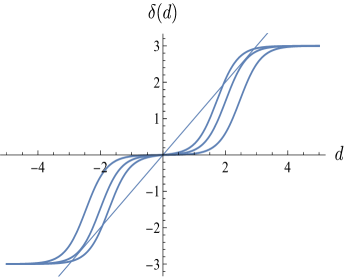
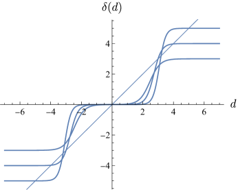
Figure 1: $\Gamma$-Minimax Rule for Model I. Left: Rules for values for $m=3$ and $\epsilon=0.5,0.7,$ and $0.9.$ Right: Rules for $\epsilon=0.9$ and $m=3,4,$ and $5$.

$\epsilon$	$m^{*}$ (Model I)	$m^{*}$ (Model II)
0.0	1.05674	0.81758
0.1	1.15020	0.91678
0.2	1.27739	1.05298
0.3	1.46988	1.25773
0.4	1.84922	1.52579
0.5	2.28384	1.74714
0.6	2.41918	1.91515
0.7	2.50918	2.05511
0.8	2.58807	2.19721
0.9	2.69942	2.40872
0.95	2.81605	2.63323
0.99	3.10039	3.24539

Table 1: Values of $m^{*}$ for both models for different values of $\epsilon.$

2.2 Model II

In Model II, the variance $\sigma^{2}$ is not known and is given an exponential prior. It is well-known that the exponential distribution is an entropy maximizer in the class of all distributions supported on $R^{+}$ with a fixed first moment. This choice is noninformative, in a form of a maxent prior.

The model is:

$$[d|\theta,\sigma^{2}]\sim{\cal N}(\theta,\sigma^{2}),$$

$$[\sigma^{2}]\sim{\cal E}(\mu),~{}~{}~{}~{}~{}\left[f(\sigma^{2})=\frac{1}{\mu}\exp\left\{-\frac{\sigma^{2}}{\mu}\right\}\right]$$

The marginal likelihood is double exponential as an exponential scale mixture of normals,

$$[d|\theta]\sim{\cal DE}\left(\theta,\sqrt{\frac{\mu}{2}}\right)~{}~{}~{}~{}\left[g(d|\theta,\mu)=\sqrt{\frac{1}{2\mu}}\exp\left\{-\sqrt{\frac{2}{\mu}}|d-\theta|\right\}\right].$$

Theorem 2. If in Model II the family of priors on the location parameter is (7), the resulting $\Gamma$-minimax rule is:

$$\delta_{B}(d)=\frac{m\left(e^{-\sqrt{2/\mu}~{}|d-m|}-e^{-\sqrt{2/\mu}~{}|d+m|}\right)}{e^{-\sqrt{2/\mu}~{}|d-m|}+\frac{2\epsilon}{1-\epsilon}e^{-\sqrt{2/\mu}~{}|d|}+e^{-\sqrt{2/\mu}~{}|d+m|}},$$ (9)

is Bayes with respect to the least favorable prior

$$[\theta]\sim\pi(\theta)=\epsilon\delta_{0}+\frac{1-\epsilon}{2}(\delta_{-m}+\delta_{m}),$$

whenever $m\leq m^{*}.$ Figure 2 shows the shinkage rule in (9) for selected values of parameters $\epsilon$ and $m$. The values of $m^{*}$ depend on $\epsilon$ and are given in Table 1 for both models. Sketches of proofs of Theorems 1 and 2 are deferred to Appendix.

  

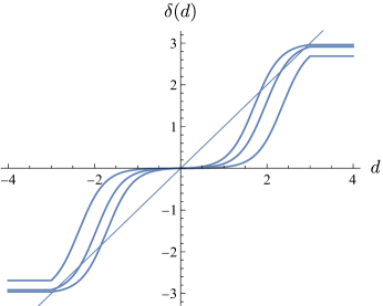
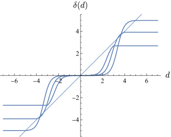
Figure 2: $\Gamma$-Minimax Rule for Model II. Left: Rules for values or $\epsilon=0.5,0.7,$ and $0.9.$ Right: Rules for $m=3,4,$ and $5$.

3.   Risk, Bias, and Variance of $\Gamma$-Minimax Rules

Frequentist risk of a rule $\delta$, as a function ot $\theta$, can be decomposed as a sum of two functions, variance and bias-squared,

$$R(\delta,\theta)=E^{d|\theta}(\delta(d)-\theta)^{2}=E^{d|\theta}(\delta(d)-E^{d|\theta}(\delta(d))^{2}+(\theta-E^{d|\theta}(\delta(d)))^{2}.$$

To explore behavior of the two risk components in the context of Models I and II, we selected the risk of $\Gamma$-minimax rule for $\epsilon=0.8$ and $m=2.197.$ (Fig. 3). This particular value of $m$ ensures that the rules are $\Gamma$-minimax (in fact $m=m^{*}$ for model II). Note that $\delta$ in Model II shows smaller risk for values of $\theta$ in the neighborhood of $m$, while for $\theta$ close to 0, the risk of the rule from Model I is smaller.

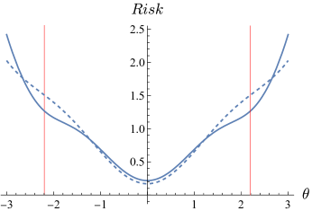
Figure 3: Risk of $\Gamma$-Minimax rule for $\epsilon=0.8$ and $m=2.197.$ Dashed plots for Model I and solid for Model II.

Similar, but less pronounced behavior is present in bias-squared function (Fig.4 Left Panel). Compared to Model I, the variance of $\delta$ in Model II is significantly smaller for values of $\theta$ in the neighborhood of $\pm m$, and larger for $\theta$ in the neighborhood of zero. Preference in using either Model I or II depends on what size of signal part we are more interested. If there is more uncertainty about signal bound $m$, the rule form Model II is preferable. However, Model I has lower risk and both components of the risk in the neighborhood of 0. This translates to a possibly more precise shrinkage of small wavelet coefficients.

  

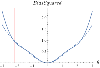
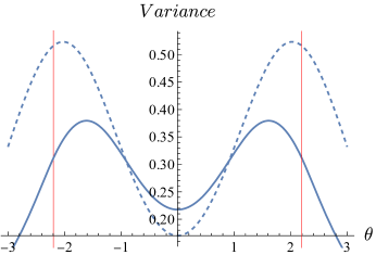
Figure 4: Risk components of $\Gamma$-minimax rule for $\epsilon=0.8$ and $m=2.197.$ Dashed plots for Model I and solid for Model II. Left: Bias-squared; Right: Variance

4.   Elicitation of Parameters

The proposed Bayesian shrinkage procedures with three-point priors depend on three parameters, $m$, $\epsilon$ and $\mu$ that need to be specified. The criteria used for selecting these parameters are critical for effective signal denoising. We propose these hyper-parameters to be elicited in an empirical Bayes fashion, that is, dependent on the observed wavelet coefficients.

• Elicitation of $m$: The bound $m$ in the domain of signal acquisition translates to level dependent bounds on the parameter $\theta$ in the wavelet domain. Given a data signal ${\mathchoice{\offinterlineskip\vtop{ \hbox{\vbox{\hbox{$\displaystyle y$}}} \vskip 1.2pt\vbox to0.4pt{ \hbox to5.2616pt{\hss\char 126\relax\hss} \vskip 0.0pt minus 1.0fil } \vskip 0.4pt}}{\offinterlineskip\vtop{ \hbox{\vbox{\hbox{$\textstyle y$}}} \vskip 1.2pt\vbox to0.4pt{ \hbox to5.2616pt{\hss\char 126\relax\hss} \vskip 0.0pt minus 1.0fil } \vskip 0.4pt}}{\offinterlineskip\vtop{ \hbox{\vbox{\hbox{$\scriptstyle y$}}} \vskip 1.2pt\vbox to0.4pt{ \hbox to3.6831pt{\hss\char 126\relax\hss} \vskip 0.0pt minus 1.0fil } \vskip 0.4pt}}{\offinterlineskip\vtop{ \hbox{\vbox{\hbox{$\scriptscriptstyle y$}}} \vskip 1.2pt\vbox to0.4pt{ \hbox to2.63078pt{\hss\char 126\relax\hss} \vskip 0.0pt minus 1.0fil } \vskip 0.4pt}}}=(y_{1},\dots,y_{n})$, the hyper-parameter $m$ at the $j^{th}$ multiresolution level is estimated as

  $$m(j)=\hat{\sigma}\max(|y_{i}|)\left(\sqrt{2}\right)^{J-j},$$ (10)

  where $J=\log_{2}n$ is the resolution level of the transformation, and $\hat{\sigma}$ an estimator of the noise size. The noise size is standardly estimated by a robust estimator of standard deviation that utilizes wavelet coefficients at the finest multiresolution level,

  $$\hat{\sigma}=\frac{\text{median}(|d_{J-1,\bullet}-\text{median}(d_{J-1,\bullet})|)}{0.6745},$$ (11)

  where $d_{J-1,\bullet}$ represents all detail coefficients in the level $J-1.$ The multiple $\left(\sqrt{2}\right)^{J-j}$ in (10) reflects the increase of the extrema of absolute value of wavelet coefficients corresponding to a signal part in $j$ steps of the transform.

• Elicitation of $\epsilon$: This parameter controls the amount of shrinkage in the neighborhood of zero and overall shape of shrinkage rule. For the levels of fine details this parameter should be close to 1. Based on the proposal for the $\epsilon$ given by Angelini and Vidakovic (2004) and Sousa et al. (2021), we suggest a level-dependent $\epsilon_{0}$ as follows:

  $$\epsilon_{0}(j)=1-\frac{1}{(j-J_{0}+l)^{k}},$$ (12)

  where $J_{0}\leq j\leq J-1$ and $k$ and $l$ are positive constants.

  As we indicated, $\epsilon$ should be close to one at the multiresolution levels of fine details, and then be decreasing gradually for levels approaching the coarsest level (Angelini and Vidakovic, 2004). When $k$ and $l$ are large, $\epsilon$ remains close to one over all levels. This results in an almost noise-free reconstruction, but could result in over-smoothing. On the other hand, $l>1$ guarantees a certain level of shrinkage even at the coarsest level. Thus, the hyperparameters $l$ and $k$ should be selected with a care in order to achieve good performance for a wide range of signals. Numerical simulations guided us to suggest values $l\geq 6$ and $k=2$ as reasonable choices. However, it is important to note that these parameters should depend on the smoothness of data signals and their size. We further discuss the selection of $l$ and $k$ for specific signals in Section 5.

• Elicitation of $\mu$: This parameter is needed only for Model II. Since the prior on the noise level $\sigma^{2}$ is exponential and the prior mean is $\mu$, by moment matching we select $\mu$ as $\hat{\sigma}^{2}$. A possible choice for $\hat{\sigma}^{2}$ is a robust estimator as in (11).

5.   Simulation Study

In the simulation study, we assessed the performance of the proposed shrinkage procedures on the battery of standard test signals. We used nine different test signals (step, wave, blip, blocks, bumps, heavisine, doppler, angles, and parabolas), which are constructed to mimic a variety of signals encountered in applications (Fig. 5). As standardly done in literature, Haar and Daubechies six-tap (Daubechies 6) were used for Blocks and Bumps and Symmlet 8-tap filter was used for the remaining test signals. The shrinkage procedures are compared using the average mean square error (AMSE), as in (13). All simulations were performed using MATLAB software and toolbox GaussianWaveDen (Antoniadis et al., 2001) that can be found at http://www.mas.ucy.ac.cy/~fanis/links/software.html.

We generated noisy data samples of the nine test signals by adding normal noise with zero mean and variance $\sigma^{2}=1$. The signals were rescaled so that $\sigma^{2}=1$ leads to a prescribed SNR. Each sample consisted of $n=1024$ data points equally spaced on the interval $[0,1]$. Figure 6 shows a noisy version of the nine test signals with SNR=1/4. Each noisy signal was transformed into the wavelet domain. After the shrinkage was applied to the transformed signal, the inverse wavelet transform was performed on the processed coefficients to produce a smoothed version of a signal in the original domain. The AMSE was computed as

$$AMSE(f(t))=\frac{1}{nN}\sum_{j=1}^{N}\sum_{i=1}^{n}\left(f(t_{i})-\hat{f}_{j}(t_{i})\right)^{2},$$ (13)

where $f$ denotes the original test signal and $\hat{f_{j}}$ its estimator in the $j$-th iteration. To calculate the average mean square error this process was repeated $N=100$ times.

Figure 5: The nine test signals used in the simulation study.

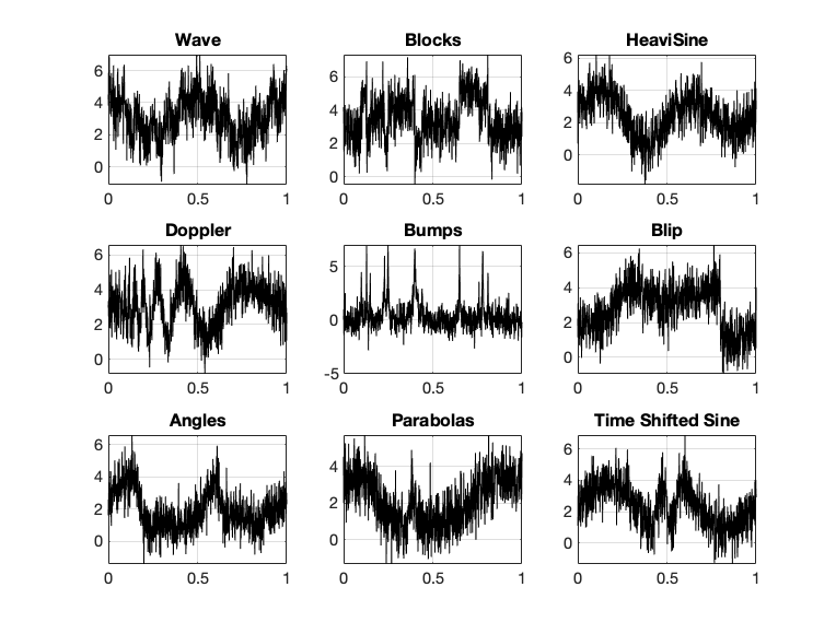
Figure 6: Noisy versions of the nine signals from Fig. 5.

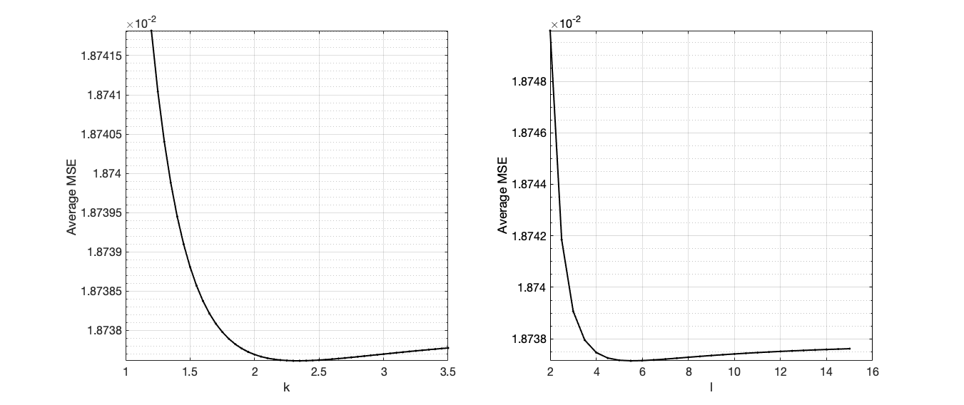
Figure 7: Change in average MSE as a function of hyper-parameters (a) $l$ and (b) $k$ exemplified on the Heavisine test signal, $SNR=1/5$, and $n=1024$.

The shrinkage procedure was applied to each test signal and the MSE was computed for a range of parameter values of $l$ and $k$. For example, Fig. 8 shows the average MSE obtained on the heavisine test signal when SNR=1/5, and $l$ and $k$ vary in the range $l\in[2,15]$ and $k\in[1.0,3.5].$ . As evident from Fig. 8, the estimator achieves its best performance for values $k\approx 2.4$ and $l\approx 5.8$. With these selected values of $l$ and $k$, Fig. 7 shows that the estimator is sufficiently close to the original test signal, even though the SNR is quite small.

Based on our simulations, the optimal hyper-parameter values of $l$ and $k$ varied depending on the nature (e.g., smoothness) of test signal. For larger values of $k$ and $l$, the estimator performs better for smooth signals. This is because the corresponding wavelet coefficients rapidly decay with the increase in resolution. However, larger values of $l$ and $k$ may not detect localized features in signals (e.g., cusps, discontinuities, sharp peaks), resulting in over-smoothing. For low values of SNR, the three-point priors estimator is more sensitive to hyper-parameter values of $l$ and $k$. When SNR increases, the estimation method shows better performance for most of the test signals with relatively small values of $l$ and $k$. Moreover, higher values of parameter $l$ and $k$ are preferred when the sample size is large.

In general, we suggest that $k=2.5$ and $l\geq 6$ as the most universal choice. The suggested values could, however, be adjusted depending on available information about the nature of signals.

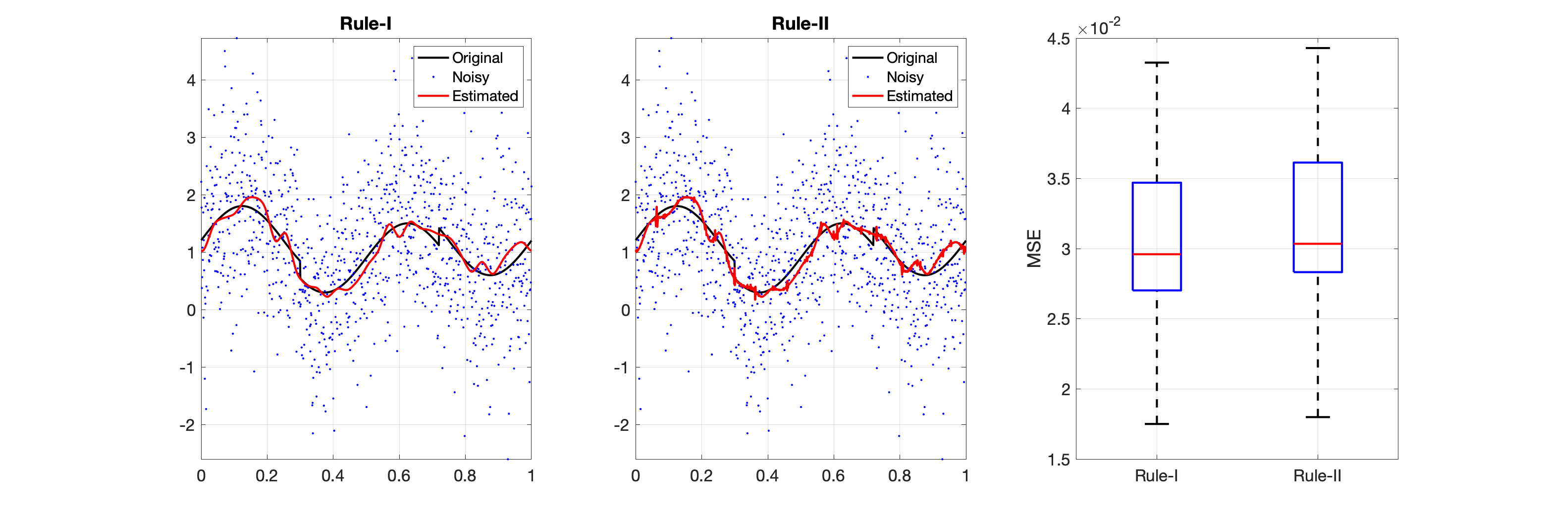
Figure 8: Estimation of heavisine test signal: Estimations obtained by three-point priors with $n=1024,k=2.4,l=5.8$ and $SNR=1/5$.

5.1 Performance Comparison with Some Existing Methods

We compared the performance of the proposed three-point prior estimator with eight existing estimation techniques. The selected existing estimation techniques include: Bayesian adaptive multiresolution shrinker (BAMS) (Vidakovic snd Ruggeri, 2001), Decompsh (Huang and Cressie, 2000), block-median and block-mean (Abramovich et al., 2002), hybrid version of the block-median procedure (Abramovich et al., 2002), blockJS (Cai, 1999), visu-shrink (Donoho and Johnstone, 1994), and generalized cross validation (Amato and Vuza, 1997). The first five techniques are relying on a Bayesian procedure and they are based on level-dependent shrinkage. The blockJS method uses a level-dependent thresholding, while the visu-shrink and generalized cross validation techniques use a global thresholding method. Readers can find more details about these techniques in Antoniadis et al. (2001).

In the simulation study, we computed the AMSE using the parameter values of $l=6$ and $k=2.5$ and compared with the AMSE computed for the selected estimation techniques. As can be seen in Fig. 9, the proposed estimator shows comparable and for some signals better performance compared to the selected estimation methods. In particular, for smooth signals (e.g., wave, heavisine), the three-point prior estimator shows better performance compared to non-smooth signals, such as blip, for instance. Moreover, when comparing the performance of the level-dependent estimation methods, the BAMS estimation method shows competitive (or better) performance for most of the cases. We also investigated the influence of SNR level and the sample size on the performance of proposed estimators, compared to the methods considered. For example, for higher SNR (Fig. 10), the three-point priors-based shrinkage procedure does not provide better performance except for wave, angels, and time shifted sine. In general, the $\Gamma$-mionimax shrinkage shows comparable or better performance compared to other methods considered, when the SNR is low. Also, for larger sample sizes, the three-point prior shrinkage shows improved performance.

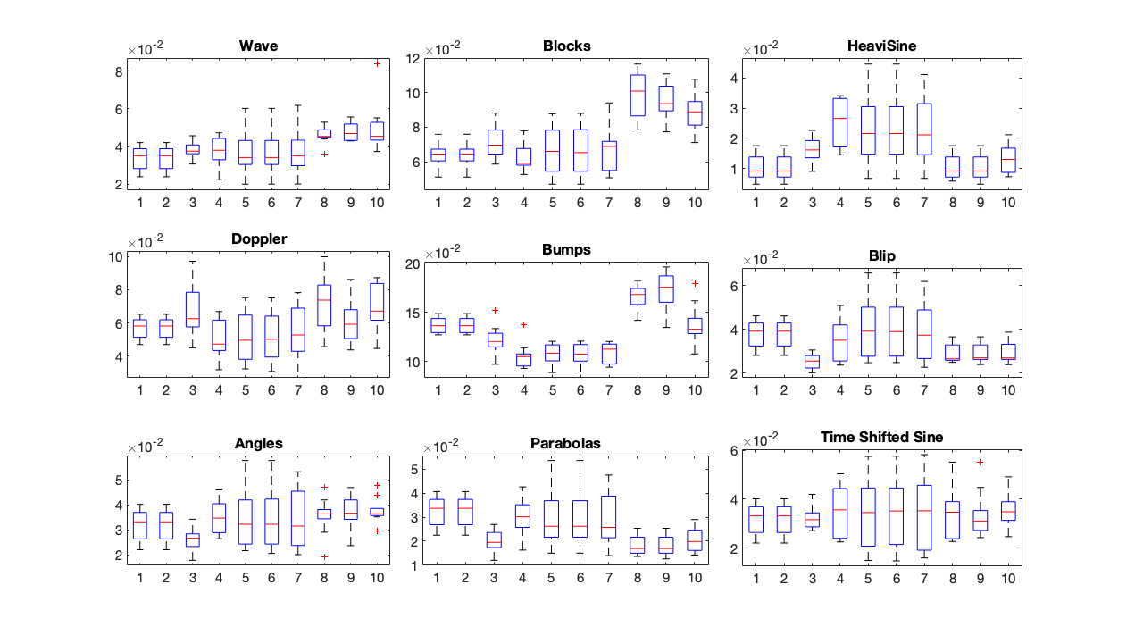
Figure 9: The box plots of MSE for the ten estimation methods: (1) Rule-I, (2) Rule-II, (3) Bayesian adaptive multiresolution shrinker (BAMS), (4) Decompsh, (5) Block-median, (6) Block-mean, (7) Hybrid version of the block-median procedure, (8) BlockJS, (9) Visu-Shrink, and (10) Generalized cross validation. The MSE was computed by using $SNR=1/5,k=2.5,l=6$, and $n=1024$ data points.

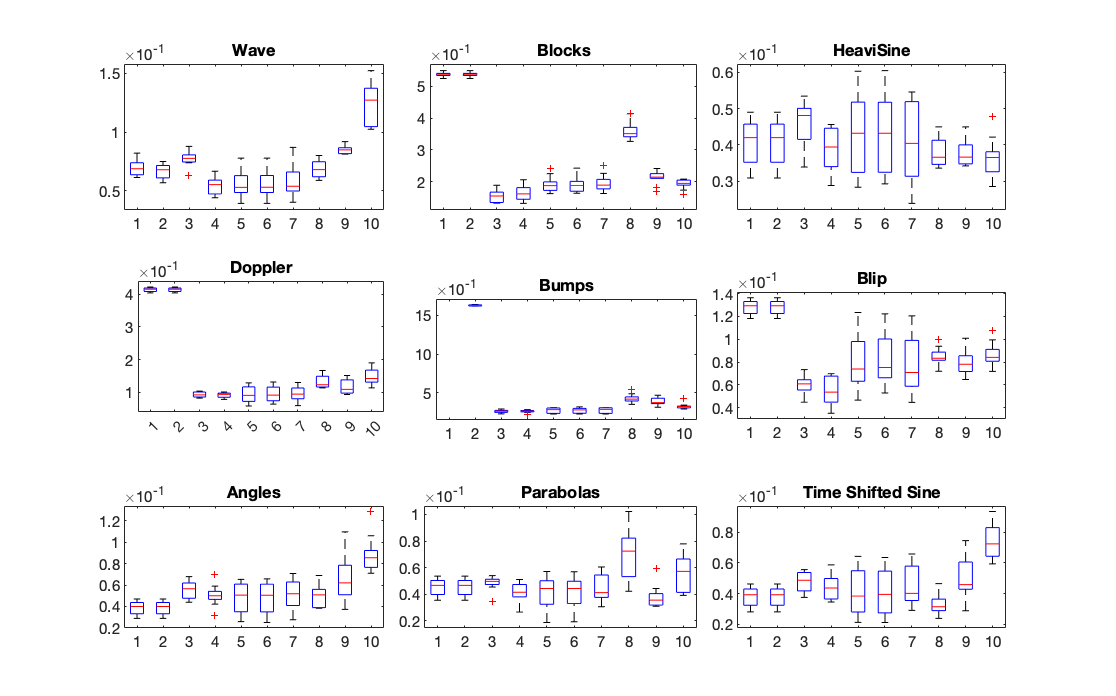
Figure 10: The same plot as in Fig. 8 with SNR = 3.

6.   Appendix

6.1 Proof of Theorem 1

Consider the class $\Gamma$ of all priors on location $\theta$ in consisting of a point mass at 0 at a fixed level $\epsilon$, and an arbitrary component $\xi(\theta)$ supported on $[-m,m]$ and nonatomic at 0,

$$\Gamma=\{\pi(\theta)=\epsilon\delta_{0}+(1-\epsilon)\xi(\theta),-m\leq\theta\leq m\}.$$

When $\epsilon=0,$ we recover the result from Casella and Strawderman (1981) for which a precise value of $m^{*}$ is $1.05674351366013496,$ to which we will refer to as Casella-Strawderman’s constant.

It is well known result (Levit, 1980; Bickel 1981) that extremal priors in the class of all distributions supported on $[-m,m]$ are symmetric distributions with point masses at 0 and pairs $-m\leq\pm m_{i}\leq m,~{}i=1,2,\dots$. Thus, in the $\Gamma$-minimax setup involving this class, the least favorable distributions are Bayes with respect to extremal priors in $\Gamma$, symmetric distributions consisting of point masses. When $m$ is small (smaller that Casella-Strawderman’s constant) the least favorable prior that puts equal weights at the endpoints $\pm m$, that is, the prior $\pi(\theta)=\frac{1}{2}\delta_{-m}+\frac{1}{2}\delta_{-m}$ is the least favorable. The statistical game $\inf_{\delta}\sup_{\pi}r(\delta,\pi)$ has a value $r(\delta^{*},\pi),$ where $\pi$ is the least favorable prior and $\Gamma$-minimax rule $\delta^{*}$ is Bayes’ rule with respect to $\pi.$

In the setup of Model I, the point mass at 0 is a part of every prior; the second component $\xi(\theta)$ is as in Casella and Strawderman (1981), but non-atomic at 0. Conditions of Sion-type theorem, allowing for change of order of inf and sup in (1), are not affected by narrowing the class $\Gamma$, the game has value, and for $m<m^{*}$ the least favorable prior is a three-point mass prior, with masses concentrated at $-m,0,$ and $m$, with weights $(1-\epsilon)/2,\epsilon,$ and $(1-\epsilon)/2.$

The corresponding Bayes rule $\delta^{*}$ is readily found by simplifying

$$\delta^{*}(d)=\frac{\int\theta f(d|\theta)\pi(\theta)d\theta}{\int f(d|\theta)\pi(\theta)d\theta}=\frac{(1-\epsilon)m/2\left[\phi(d|m)-\phi(d|-m)\right]}{\epsilon\phi(d|0)+(1-\epsilon)/2\left[\phi(d|m)+\phi(d|-m)\right]},$$

where $\phi(d|\mu)$ is the pdf of normal ${\cal N}(\mu,1)$ distribution. A simplified expression is given in (8).

To find values of $m^{*}$ so that for $m\leq m^{*}$ the three point prior is least favorable, we analyze the freqentist risk, $R(\theta,\delta^{*})=E^{d\theta}(\theta-\delta^{*})^{2},$ for a fixed $\epsilon,$ by varying $m^{*}.$ Depending on $\epsilon,$ there are three possible shapes of the frequentist risk, which we denote as W, VVV, and V. Numerical work shows that values of $\epsilon$ that separate these three shapes are $\epsilon_{1}\approx 0.45$ and $\epsilon_{2}\approx 0.65.$

For small values of $\epsilon$, ($<\epsilon_{1}$) the risk $R(\theta,\delta^{*})$ is of W-shape, as in the left panel of Fig. 11.

  

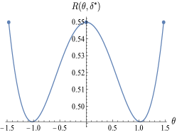
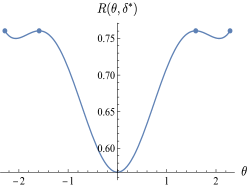
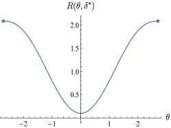
Figure 11: Model I: Frequentist risks of W-, VVV-, and V-shape, $R(\theta,\delta^{*})$, for $\epsilon=0.3$ (left), $0.5$ (middle), and $0.9$ (right).

This is a typical shape for a risk of the least favorable distribution in a class of all bounded on $[-m,m]$ distributions, for $m$ small. The value $m^{*}$ in this case is found form $R(0,\delta*)=R(-m^{*},\delta^{*})=R(-m^{*},\delta^{*}).$ If $m>m^{*},$ the risk local maximum at 0 will exceed values at $\pm m$, and one could select a prior from $\Gamma$ for which the payoff $r(\delta^{*},\pi)>r(\delta^{*},\pi_{m^{*}}.$ Note that in increasing $m$ in the search of this limiting $m^{*}$, the rule $\delta^{*}$ is simultaneously changing, since it depends on $m$, so the numerical work to find $m^{*}$ is nontrivial.

For values of $\epsilon$ between $\epsilon_{1}$ and $\epsilon_{2}$, the shape of frequentist risk is of VVV-type, as it is shown in middle panel of Fig. 11. In this case two local maximums for the frequentist risk appear at a pair of $\theta=\pm m_{1},m_{1}\leq m^{*}$. In the critical case that defines the $m^{*}$, $R(-m^{*},\delta^{*})=R(-m_{1},\delta^{*})=R(m_{1},\delta^{*})=R(m^{*},\delta^{*})$, and increasing $m$ above such $m^{*}$ will result in $R(\pm m^{*},\delta_{B})<R(\pm m_{1},\delta_{B}).$ Placing more mass at $\pm m_{1}$ will result in higher payoff $r$ and the three point prior is not the least favorable any longer.

The case when $\epsilon>\epsilon_{2}$ is most interesting since in the wavelet shrinkage, values of $\epsilon$ closer to 1 produce shrinkage rules of desirable shape. In this case, the frequentist risk is V-shaped, which flattens at the endpoints for $m=m^{*},$ that is,  $\partial R/\partial\theta\left|{}_{\theta=m^{*}}=0\right.$  (the right panel in Fig. 11). In this case if we let $m=m^{**}>m*$ the frequentist risk will start to decrease, so a prior with point masses that remain in now inner points $m^{*}$ will increase the payoff function $r$, and the three point prior with masses at $0,\pm m^{**}$ will not be the least favorable any longer.

6.2 Proof of Theorem 2.

In Model II the normal likelihood is replaced by double exponential marginal likelihood, after $\sigma^{2}$ is integrated out. Meleman and Ritov (1987) show that in estimating bounded normal mean normality of the likelihood is not necessary condition for $\Gamma$-minimax results to remain valid, if mild moment conditions on the likelihood are imposed. In fact they show that if the likelihood has a finite fourth moment, the rescaled asymptotic (when $m\rightarrow\infty$) $\Gamma$-minimax solution has the same least favorable limiting distribution, as for the normal likelihood (Bickel, 1981).

In Model II there are two common shapes of the freqientist risk, W- and VVV-shape, for $\epsilon\leq\epsilon_{1}$ and $\epsilon>\epsilon_{1},$ respectively, with $\epsilon_{1}$ between 0.3 and 0.4.

  

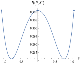
Figure 12: Model II: Frequentist risk of the $\Gamma$-minimax rule, $R(\theta,\delta^{*})$, for $\epsilon=0.2$ (Left), $0.4$ (Middle), and $0.9$ (Right).

The argument is similar as in Model I, for the W-shape (Left panel in Fig.12), a slight increase of $m$ over $m^{*}$ will make $R(\delta^{*},0)>R(\delta^{*},\pm m)$ and one can choose $\pm m_{1}$ in the neighborhood of 0, so that transferring some point mass from endpoints to $\pm m_{1}$ would increase the payoff. The argument for VVV-shaped risk (Middle and Right Panels in Fig. 12) is the same as in the Model I.

REFERENCES

Abramovich, F, Besbeas, P., and Sapatinas, T. (2002). Empirical Bayes approach to block wavelet function estimation. Comput. Statist. Data Anal., 39, 435–451.

Amato, U. and Vuza, D.T. (1997). Wavelet approximation of a function from samples affected by noise. Rev. Roumanie Math. Pure Appl., 42, 481–493.

Angelini, C. and Vidakovic, B. (2004). $\Gamma$-minimax wavelet shrinkage: A robust incorporation of information about energy of a signal in denoising applications. Stat. Sin., 14, 1, 103–125.

Antoniadis, A., Bigot, J. and Sapatinas, T. (2001). Wavelet estimators in nonparametric regression: A comparative simulation study. J. Statist. Soft., 6, 1–83.

Berger, J.O. (1984). The robust Bayesian viewpoint. In Robustness of Bayesian Analysis, (J. Kadane Eds.) Elsevier Science Publisher, 63–124.

Berger, J.O. (1985). Statistical Decision Theory and Bayesian Analysis. Springer Verlag, New York.

Bickel, P.J., (1981). Minimax estimation of the mean of a normal distribution when the parameter space is restricted. Ann. Statist., 9, 1301–1309.

Cai, T.T. (1999). Adaptive wavelet estimation: A block thresholding and oracle inequality approach. Ann. Statist., 27, 3, 898–924.

Casella, G. and Strawderman, W. (1981). Estimating a bounded normal mean. Ann. Statist., 9, 870–878.

Donoho, D.L., Liu, R., and MacGibbon, B. (1990). Minimax risk over hyperrectangles. Ann. Statist., 18, 1416-1437.

Donoho, D.L. and Johnstone, I.M. (1994). Ideal spatial adaptation via wavelet shrinkage. Biometrika, 81, 425–455.

Good, I.J. (1952). Rational decisions. J. Royal Statist. Soc. B, 14, 107–114.

Huang H.C. and Cressie, N., (2000). Deterministic/stochastic wavelet decomposition for recovery of signal from noisy data. Technometrics, 42, 262–276.

Levit, B. (1980). On asymptotic minimax estimators of second order. Theory Probab. Appl., 25, 552–568.

Meleman, A. and Ritov, Y. (1987). Minimax estimation of the mean of a general distribution when the parameter space is restricted. Ann. Statist., 15,1, 432–442.

Reményi, N. and Vidakovic, B. (2013). Bayesian wavelet shrinkage strategies: A review. In Multiscale Signal Analysis and Modeling, Springer, NY, 317–346.

Robbins, H. (1951). Asymptotically sub-minimax solutions to compound statistical decision problems. In Proc. Second Berkeley Symposium Math. Statist. and Prob., 1, 241-259. University of California Berkeley Press.

Sousa, A.R.S., Garcia, N.L., and Vidakovic, B., (2021). Bayesian wavelet shrinkage with beta priors. Comput. Stat., 36, 1341–1363.

Vidakovic, B. (2000). $\Gamma$-minimax: A paradigm for conservative robust Bayesians. In Robust Bayesian Analysis (D. Rios Insua and F. Ruggeri, eds.), Lec. Notes Statist. 152 Springer-Verlag, New York.

Vidakovic, B., and DasGupta, A., (1996). Efficiency of linear rule for estimating a bounded normal mean. Sankhya A, 58, 81–100.

Vidakovic, B. and Ruggeri, F. (2001). BAMS Method: Theory and Simulations. Sankhya B, 63, 234–249.