Gravitational waves and monopoles dark matter from first-order phase transition

Abstract

We study the possibility of monopoles serving as dark matter when they are produced during the first-order phase transition in the dark sector. Our study shows that dark monopoles can contribute only a small piece of dark matter relic density within parameter spaces where strong gravitational waves can be probed by ET and CE, and the monopoles can contribute a sizable component of the observed dark matter relic density for fast phase transitions with short duration.

I Introduction

Gravitational waves astronomy provides a new window to probe new physics beyond Standard Model that can accommodate first-order phase transitions Caldwell et al. (2022). The vector gauge bosons can serve as dark matter after the spontaneously broken of a hidden non-abelian gauge theory Hambye (2009); Arina et al. (2010); Carone and Ramos (2013). Refs. Ghosh et al. (2021); Prokopec et al. (2019); Baldes and Garcia-Cely (2019) studied phase transition within hidden non-abelian gauge theories and found the gravitational waves from the high-scale first-order phase transition can be probed by LIGO and future space-based gravitational wave detectors. Ref. Borah et al. (2021) investigated the possibility to search MeV-scale phase transition in such framework and found the parameter spaces that allowed first-order phase transition can be constrained by NanoGrav. When the non-abelian gauge theory is broken to an abelian gauge theory with the vacuum manifold being $\pi_{2}(SU(2)/U(1))=\mathbb{Z}$, dark matter might be ’t Hooft-Polyakov monopoles ’t Hooft (1974); Polyakov (1974) that are produced during cosmological phase transitions Kibble (1976); Zurek (1985). Monopoles serving as topological dark matter have been studied in Refs. Nakagawa et al. (2021); Graesser et al. (2022); Fan et al. (2021); Graesser and Osiński (2020); Daido et al. (2020); Sato et al. (2018); Kawasaki et al. (2016); Hiramatsu et al. (2021); Gomez Sanchez and Holdom (2011); Nomura et al. (2016); Nakagawa et al. (2021); Murayama and Shu (2010); Evslin and Gudnason (2012); Terning and Verhaaren (2019); Khoze and Ro (2014); Baek et al. (2014); Bai et al. (2020).

Previous studies Khoze and Ro (2014); Baek et al. (2014); Bai et al. (2020) mostly focus on monopole dark matter from second-order phase transitions. We focus on the dark monopoles formed when dark vacuum bubbles collided during the first-order phase transition Einhorn and Sato (1981); Izawa and Sato (1982). We study heavy monopoles’ contribution to dark matter relic density when the monopoles are produced during high-scale first-order phase transitions to be probed by LISA Amaro-Seoane et al. (2017), TianQin Luo et al. (2016); Hu et al. (2018); Mei et al. (2021), Taiji Hu and Wu (2017); Ruan et al. (2020), DECIGO Seto et al. (2001); Kudoh et al. (2006), and BBO Ungarelli et al. (2005); Cutler and Harms (2006), LIGO-Virgo Thrane and Romano (2013); Aasi et al. (2015); Abbott et al. (2016, 2019), CE Reitze et al. (2019), and ET Punturo et al. (2010); Hild et al. (2011); Sathyaprakash et al. (2012). We investigate the effects of phase transition duration and phase transition temperature on dark monopoles dark matter relic density.

II The dark $SU(2)_{D}$ phase transition

The spontaneous breaking of a $SU(2)_{D}$ gauge theory with a scalar field in the adjoint representation may contain ’t Hooft-Polyakov magnetic monopoles ’t Hooft (1974) when the homotopy group satisfies $\pi_{2}[SU(2)/U(1)]=\mathbb{Z}$. The relevant Lagrangian is given by,

$$\mathcal{L}=-\frac{1}{4}F_{\mu\nu}^{a}F^{\mu\nu a}+\frac{1}{2}D_{\mu}\phi^{a}D^{\mu}\phi^{a}-V(\phi)\;.$$ (1)

Therein, the field strength of the $SU(2)$ field $A_{\mu}$ is $F_{\mu\nu}^{a}=\partial_{\mu}A_{\nu}^{a}-\partial_{\nu}A_{\mu}^{a}+g_{D}\epsilon^{abc}A_{\mu}^{b}A_{\nu}^{c}\;$, the kinetic term is $D_{\mu}\phi^{a}=\partial_{\mu}\phi^{a}+g_{D}\epsilon^{abc}A_{\mu}^{b}\phi^{c}$ with the $g_{D}$ being the gauge coupling constant and $\phi^{a}(a=1,2,3)$ being the adjoint scalars, the tree-level potential at zero temperature is

$$V(\phi)=-\frac{m^{2}}{2}\phi^{a}\phi^{a}+\frac{\lambda_{\phi}}{4}(\phi^{a}\phi^{a})^{2}\;.$$ (2)

At zero temperature, the vacuum expectation value $v=w=m/\sqrt{\lambda_{\phi}}$ is the minimum of the potential $V$. After symmetry breaking, we get two massive gauge bosons $W_{\pm}^{\prime}$ with mass $m_{W^{\prime}}=g_{D}w$, one massless gauge boson $\gamma^{\prime}$ and one massive scalar with $m_{\phi}=\sqrt{2}m$.

To investigate the phase transition process that leads to the symmetry breaking of $SU(2)_{D}\to U(1)_{D}$, we study the thermal effective potential at the one-loop level by considering high-temperature approximation Quiros (1994), which takes the form as Khoze and Ro (2014):

$$V_{T}(\phi)=D(T^{2}-T_{0}^{2})\phi^{a}\phi^{a}-ET(\phi^{a}\phi^{a})^{3/2}+\frac{\lambda_{T}}{4}(\phi^{a}\phi^{a})^{2}\;.$$ (3)

The relevant parameters are: $D=g_{D}^{2}/4,\ E=g_{D}^{3}/2\pi,\ T_{0}^{2}=\left(\sqrt{2}m^{2}-g_{D}^{4}w^{2}/2\pi\right)/(4D),\lambda_{T}=\lambda_{\phi}-3g_{D}^{4}/8\pi^{2}\log(g_{D}^{2}w^{2}/a_{B}T^{2})\;$ with $a_{B}\simeq e^{3.91}$. Below the critical temperature, the phase transition would take place when at least one bubble is nucleated per horizon volume and per horizon time, which can be defined as Affleck (1981); Linde (1983, 1981):

$$\Gamma\approx A(T_{n})e^{-S_{3}/T_{n}}\simeq 1\;.$$ (4)

Where $T_{n}$ is the nucleation temperature of the vacuum bubbles, and $S_{3}$ is the bounce action for an O(3) symmetric bounce solution that can be written as

$$S_{3}(T)=\int 4\pi r^{2}dr\bigg{[}\frac{1}{2}\big{(}\frac{d\phi_{b}}{dr}\big{)}^{2}+V_{T}(\phi_{b})\bigg{]}\;,$$ (5)

with $\phi_{b}=\phi$ in our case, and $V_{T}(\phi_{b})$ is the thermal effective potential in Eq.3. The bubble nucleation events would be generated when one gets the bounce solution from solving the equations of motion for $\phi_{b}$:

$$\frac{d^{2}\phi_{b}}{dr^{2}}+\frac{2}{r}\frac{d\phi_{b}}{dr}-\frac{\partial V(\phi_{b})}{\partial\phi_{b}}=0\;,$$ (6)

with the boundary conditions being

$$\lim_{r\rightarrow\infty}\phi_{b}=0\;,\quad\quad{\left.{\frac{{d{\phi_{b}}}}{{dr}}}\right|_{r=0}}=0\;.$$ (7)

One typical parameter is the phase transition strength $\alpha$, which can be calculated based on the trace of the energy-momentum tensor Giese et al. (2020, 2021); Guo et al. (2021):

$$\alpha=\frac{1}{3\omega_{s}}((1+\frac{1}{c^{2}_{s}})\Delta V_{eff}-T\frac{d\Delta V_{eff}}{dT})|_{T=T_{n}}\;,$$ (8)

where $\omega$ is the enthalpy density, and subscripts $``s"$ indicate the quantities outside the bubbles. $\Delta V_{eff}$ is the thermal effective potential difference between the symmetric and broken phase. The speed of sound $c_{s}$ is defined as: $c_{s}^{2}=(dp/dT)/(de/dT)$, where $e$ ($p$) is the energy density (the pressure). Another typical parameter $\beta$ which characterizes the inverse duration of the first-order phase transition (in units of Hubble) can be obtained as $\beta/H_{n}=\left.Td(S_{3}(T)/T)/(dT)\right|_{T=T_{n}}\;$ with $H_{n}$ being the Hubble constant at the nucleation temperature $T_{n}$.

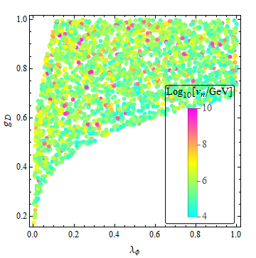
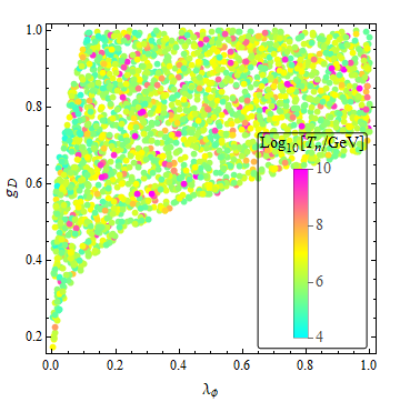
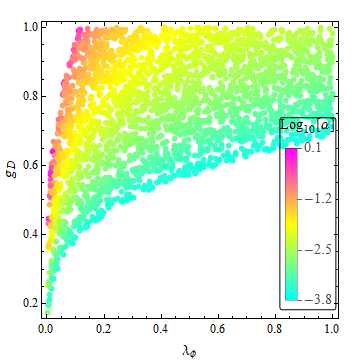
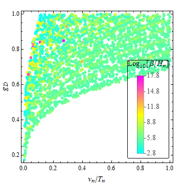
Figure 1: The top two plots show the $v_{n}$ and $T_{n}$ for phase transitions with different model parameters; and the bottom two plots depict the values of phase transition strength $\alpha$ and inverse phase transition duration $\beta/H_{n}$.

With the above procedure, we scan model parameters of $g_{D}\sim[0,1],w\sim[10^{5},10^{10}]$ GeV, $\lambda_{\phi}\sim[0,1]$ to find bounce solutions by utilizing FindBounce Guada et al. (2020), and calculate the phase transition strength and duration. Our results are shown in Fig. 1. The top two plots present the distributions of the background field value ($v_{n}$) at the nucleation temperature ($T_{n}$), both $v_{n}$ and $T_{n}$ range from $10^{4}$ GeV to $10^{10}$ GeV. The yielded phase transition strength $\alpha$ and the inverse phase transition duration ($\beta/H_{n}$) are shown in the bottom two panels respectively. In most parameter spaces, we have weak phase transition with $\alpha<0.1$ and large $\beta/H_{n}$, where stronger phase transition strength $\alpha$ can be obtained with smaller $\lambda_{\phi}$ and larger $g_{D}$. As will be studied later, dark monopoles generated during the phase transition with larger $\beta$ can contribute more dark matter relic density, and the strong gravitational wave requires relatively small $\beta/H_{n}$ and strong phase transition with a large $\alpha$.

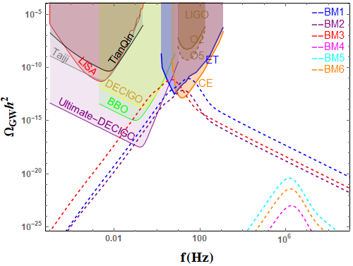
Figure 2: Gravitational wave spectra for phase transition benchmarks in Table. 1.

A first-order PT occurs when dark vacuum bubbles nucleated and merged with each other as the temperature of the Universe drops. Gravitational waves could then be generated, with the spectrum of gravitational wave can be obtained systematically Caprini et al. (2020). Generically, the prediction of the gravitational wave spectrum depends on four crucial parameters: the bubble wall velocity $v_{w}$, the phase transition temperature (we take $T_{n}$ in this study), the phase transition strength $\alpha$, and the inverse phase transition duration $\beta$. In this work, we consider three sources of gravitational waves during the dark first-order PT: 1) the bubble collision, here we take the widely used envelop approximation  Kosowsky et al. (1992a, b); Kosowsky and Turner (1993); Kamionkowski et al. (1994); Huber and Konstandin (2008) (see also Child and Giblin (2012) and analytic estimations Jinno and Takimoto (2017)); 2) the sound waves in the plasma Hindmarsh et al. (2014, 2015), and 3) the magnetohydrodynamic turbulence (MHD) Hindmarsh et al. (2014, 2015), which may subdominant when a small fraction of the energy flows into the MHD Caprini et al. (2009); Binetruy et al. (2012). In Fig. 2, we present the gravitational wave predictions for several benchmarks given in Table. 1. Where we find that large $\beta/H_{n}$ (and small $\beta/H_{n}$) yield low (and high) magnitude of GWs. The possibility of the monopoles serving as DM in these benchmarks will be studied below.

BM	$g_{D}$	$\leavevmode\nobreak\ \leavevmode\nobreak\ \lambda_{\phi}$	$w(\text{GeV})$	$\leavevmode\nobreak\ \leavevmode\nobreak\ T_{n}(\text{GeV})$	$\alpha$	$\beta/H_{n}$
$BM_{1}$	$0.99$	$0.11$	$2.77\times 10^{6}$	$3.21\times 10^{5}$	$1.28$	$754.07$
$BM_{2}$	$0.64$	$0.02$	$6.82\times 10^{5}$	$6.31\times 10^{4}$	$0.90$	$2213.46$
$BM_{3}$	$0.57$	$0.01$	$6.77\times 10^{5}$	$5.97\times 10^{4}$	$0.81$	$640.42$
$BM_{4}$	$0.66$	$0.63$	$4.87\times 10^{7}$	$6.97\times 10^{7}$	$4.26\times 10^{-4}$	$2.20\times 10^{5}$
$BM_{5}$	$0.92$	$0.61$	$6.93\times 10^{7}$	$6.88\times 10^{7}$	$5.12\times 10^{-3}$	$1.79\times 10^{5}$
$BM_{6}$	$0.87$	$0.70$	$4.16\times 10^{7}$	$4.74\times 10^{7}$	$2.73\times 10^{-3}$	$2.87\times 10^{5}$

Table 1: The benchmark points for gravitational waves and dark monopoles.

III Monopole dark matter

When the phase transition occurs, monopoles can be formed with a rate of $p\sim\mathcal{O}(10^{-1})$ after dark vacuum bubbles collided with each other. The monopole density $n_{m,*}$ can be related to the bubble number density $n_{b,*}$ through the following relation Einhorn and Sato (1981),

$$n_{m,*}=pn_{b,*}=p\frac{\beta^{3}}{8\pi v_{w}^{3}}\;.$$ (9)

When monopoles are formed, configurations of the dark scalar and dark gauge fields are as follows Hiramatsu et al. (2021):

$$\phi^{a} = v_{n}H(r)\frac{x^{a}}{r}\;,$$

$$A_{i}^{a} = \frac{1}{g_{D}}\frac{\epsilon^{aij}x^{j}}{r^{2}}F(r)\;,\ \ (i,j=1,2,3),$$ (10)

where $\epsilon^{aij}$ is the anti-symmetric tensor with a convention $\epsilon^{123}=1$, and $r=\sqrt{x^{2}+y^{2}+z^{2}}$. In terms of the above configurations, the Lagrangian given in Eq.1 reduces to

$$L = \int\mathcal{L}d^{3}x=-4\pi\int_{0}^{\infty}r^{2}dr\bigg{[}\frac{1}{g_{D}^{2}r^{2}}\left(\frac{dF}{dr}\right)^{2}$$ (11)

$$+ \frac{2F^{2}(1-F)}{g_{D}^{2}r^{4}}+\frac{F^{4}}{2g_{D}^{2}r^{4}}+\frac{v_{n}^{2}}{2}\left(\frac{dH}{dr}\right)^{2}$$

$$+ \frac{v_{n}^{2}H^{2}}{r^{2}}(1-F)^{2}+V_{T}(H)\bigg{]}\;.$$

Introducing the dimensionless variable $\xi=v_{n}r$, we have

$$L = -\frac{4\pi v_{n}}{g_{D}^{2}}\int_{0}^{\infty}d\xi\bigg{[}\left(\frac{dF}{d\xi}\right)^{2}+\frac{2F^{2}(1-F)}{\xi^{2}}$$ (12)

$$+ \frac{F^{4}}{2\xi^{2}}+\frac{g_{D}^{2}\xi^{2}}{2}\left(\frac{dH}{d\xi}\right)^{2}+g_{D}^{2}H^{2}(1-F)^{2}$$

$$+ \frac{g_{D}^{2}V_{T}(H)}{v_{n}^{4}}\xi^{2}\bigg{]}.$$

Then, equations of motion of the system can be obtained as:

$$\frac{d^{2}F}{d\xi^{2}}=\frac{F}{\xi^{2}}(1-F)(2-F)+g_{D}^{2}H^{2}(F-1)\;,$$ (13)

$$\frac{d^{2}H}{d\xi^{2}}+\frac{2}{\xi}\frac{dH}{dx}=\frac{2H}{\xi^{2}}(1-F)^{2}+\frac{1}{v_{n}^{4}}\frac{dV_{T}(H)}{dH}\;.$$ (14)

Where, the functions $H(\xi)$ and $F(\xi)$ satisfy boundary conditions:

$$\lim_{\xi\to 0}H(\xi)\rightarrow 0\;,\ \ \ \ \lim_{\xi\to\infty}H(\xi)\rightarrow 1\;,$$ (15)

$$\lim_{\xi\to 0}F(\xi)\rightarrow 0\;,\ \ \ \ \lim_{\xi\to\infty}F(\xi)\rightarrow 1\;.$$ (16)

After the $H(\xi)$ and $F(\xi)$ are solved numerically, we can obtain the mass of the monopole as

$$M_{m} = \int[-\mathcal{L}-V_{T}(v_{n})]d^{3}x$$ (17)

$$= \frac{4\pi v_{n}}{g_{D}^{2}}\int_{0}^{\infty}d\xi\bigg{[}\left(\frac{dF}{d\xi}\right)^{2}+\frac{2F^{2}(1-F)}{\xi^{2}}$$

$$+ \frac{F^{4}}{2\xi^{2}}+\frac{g_{D}^{2}\xi^{2}}{2}\left(\frac{dH}{d\xi}\right)^{2}+g_{D}^{2}H^{2}(1-F)^{2}$$

$$+ \frac{g_{D}^{2}V_{T}(H)}{v_{n}^{4}}\xi^{2}-\frac{g_{D}^{2}V_{T}(H=1)}{v_{n}^{4}}\xi^{2}\bigg{]}.$$

The relic density of dark monopoles can be calculated as

$$\Omega_{M}=\frac{\rho_{M,0}}{\rho_{crit,0}}=\frac{M_{m}n_{m,*}s_{0}}{3M_{pl}^{2}H_{0}^{2}s_{*}},$$ (18)

where $s_{*}$ is the entropy density of the universe at the temperature of phase transition, $s_{0}$ is the entropy density today and $H_{0}$ is the current Hubble constant. Utilizing the relation $s(T)=\frac{2\pi^{2}}{45}g_{s}(T)T^{3}$, we have the dark monopole dark matter relic density

$$\Omega_{DM}h^{2}=pM_{m}\frac{\beta^{3}g_{s}(T_{0})T_{0}^{3}h^{2}}{24\pi v_{w}^{3}g_{s}(T_{n})T_{n}^{3}M_{pl}^{2}H_{0}^{2}},$$ (19)

where $g_{s}$ is the effective number of degrees of freedom in entropy.

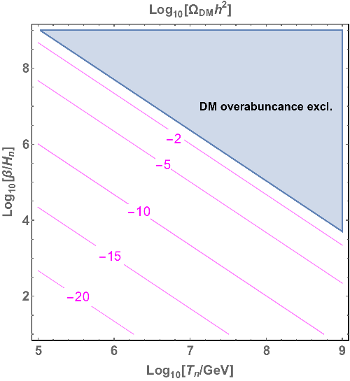
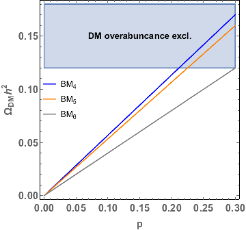
Figure 3: Monopoles dark matter relic density. In left panel, we present the monopoles dark matter relic abundance as functions of $\beta$ and phase transition temperature $T_{n}$ with bubble velocity $v_{w}=1$ and monopole generation rate $p=0.1$. In the right plot, we show the dark matter relic density for three benchmarks in Table. 1.

In the left plot of Fig. 3, for illustration, we take $M_{m}\sim 4\pi v_{n}/g_{D}^{2}\sim 4\pi T_{n}$ since most phase transition points concentrate around $v_{n}/T_{n}\sim 1$ with $g_{D}\sim[0.5,1]$. The figure depicts that the dark matter relic density increases with increase of $\beta/H_{n}$ and the phase transition temperature $T_{n}$. The parameter spaces with long phase transition duration (i.e., a small $\beta/H_{n}$) that can produce strong gravitational waves (see $BM_{1,2,3}$ in the Fig. 2) yield negligible contributions to the dark matter relic density. The right plot shows that the short phase transition duration cases of $BM_{4,5,6}$ (with large $\beta/H_{n}$) can contribute even most part of the observed dark matter relic density depending on the monopole generation rate when dark vacuum bubbles collided with each other. Where, the monopole mass was calculated through Eq. 17 after we obtained the profiles of $H(\xi)$ (solid) and $F(\xi)$ (dotted) for the $BM_{4,5,6}$ that satisfy Eq. 13, see Fig. 4. Fig. 4 shows that both $H(\xi)$ and $F(\xi)$ approach unity for large $\xi$. After the $SU(2)_{D}$ is broken to a $U(1)_{D}$ theory, the dark photon $\gamma^{\prime}$ didn’t get mass during the phase transition, which will contribute to the effective neutrino number. Following Refs. Ghosh et al. (2021); Khoze and Ro (2014), we obtain $\Delta N_{\text{eff}}(T_{\text{CMB}})\approx 0.055,\Delta N_{\text{eff}}(T_{\text{BBN}})\approx 0.202$ that will be tested by future CMB Stage IV experiments Borah et al. (2021).

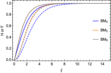
Figure 4: The profiles of $H(\xi)$(solid lines) and $F(\xi)$(dashed lines). The blue, orange, and gray lines correspond to three benchmarks in the Table. 1 respectively.

IV Conclusion and discussions

In this paper, we investigated the possibility of dark monopoles serving as dark matter and its associated gravitational waves production during the dark first-order phase transition. Our study shows that the monopoles produced during the phase transition can contribute part of the dark matter relic density depending on phase transition properties. We find heavy monopoles produced from short duration high-scale phase transitions, that produce weak gravitational waves, can contribute considerable components of the dark matter relic density. Meanwhile, we observe that for the parameter spaces with strong gravitational waves to be probed by CE and ET, the monopoles can only contribute a negligible piece of the observed dark matter relic density.

In this paper, we didn’t consider large production rates of monopoles therein one needs to consider monopole-anti-monopole annihilation for the study of dark matter relic density, see Refs. Khoze and Ro (2014); Baek et al. (2014); Bai et al. (2020) for example. The exact production of the monopoles would rely on the bubbles merging process during the first-order phase transition, we left the study to future lattice simulations.

V Acknowledgement

The work is supported by the National Key Research and Development Program of China Grant No. 2021YFC2203004. The work of Ligong Bian is supported in part by the National Natural Science Foundation of China under the grants Nos.12075041, 12047564, the Fundamental Research Funds for the Central Universities of China (No. 2021CDJQY-011 and No. 2020CDJQY-Z003), and Chongqing Natural Science Foundation (Grants No.cstc2020jcyj-msxmX0814).

References

- Caldwell et al. (2022) R. Caldwell et al., (2022), arXiv:2203.07972 [gr-qc] .
- Hambye (2009) T. Hambye, JHEP 01, 028 (2009), arXiv:0811.0172 [hep-ph] .
- Arina et al. (2010) C. Arina, T. Hambye, A. Ibarra, and C. Weniger, JCAP 03, 024 (2010), arXiv:0912.4496 [hep-ph] .
- Carone and Ramos (2013) C. D. Carone and R. Ramos, Phys. Rev. D 88, 055020 (2013), arXiv:1307.8428 [hep-ph] .
- Ghosh et al. (2021) T. Ghosh, H.-K. Guo, T. Han, and H. Liu, JHEP 07, 045 (2021), arXiv:2012.09758 [hep-ph] .
- Prokopec et al. (2019) T. Prokopec, J. Rezacek, and B. Świeżewska, JCAP 02, 009 (2019), arXiv:1809.11129 [hep-ph] .
- Baldes and Garcia-Cely (2019) I. Baldes and C. Garcia-Cely, JHEP 05, 190 (2019), arXiv:1809.01198 [hep-ph] .
- Borah et al. (2021) D. Borah, A. Dasgupta, and S. K. Kang, JCAP 12, 039 (2021), arXiv:2109.11558 [hep-ph] .
- ’t Hooft (1974) G. ’t Hooft, Nucl. Phys. B 79, 276 (1974).
- Polyakov (1974) A. M. Polyakov, JETP Lett. 20, 194 (1974).
- Kibble (1976) T. W. B. Kibble, J. Phys. A 9, 1387 (1976).
- Zurek (1985) W. H. Zurek, Nature 317, 505 (1985).
- Nakagawa et al. (2021) S. Nakagawa, F. Takahashi, and M. Yamada, Phys. Rev. Lett. 127, 181103 (2021), arXiv:2103.08153 [hep-ph] .
- Graesser et al. (2022) M. L. Graesser, I. M. Shoemaker, and N. T. Arellano, JHEP 03, 105 (2022), arXiv:2105.05769 [hep-ph] .
- Fan et al. (2021) J. Fan, K. Fraser, M. Reece, and J. Stout, Phys. Rev. Lett. 127, 131602 (2021), arXiv:2105.09950 [hep-ph] .
- Graesser and Osiński (2020) M. L. Graesser and J. K. Osiński, JHEP 11, 133 (2020), arXiv:2007.07917 [hep-ph] .
- Daido et al. (2020) R. Daido, S.-Y. Ho, and F. Takahashi, JHEP 01, 185 (2020), arXiv:1909.03627 [hep-ph] .
- Sato et al. (2018) R. Sato, F. Takahashi, and M. Yamada, Phys. Rev. D 98, 043535 (2018), arXiv:1805.10533 [hep-ph] .
- Kawasaki et al. (2016) M. Kawasaki, F. Takahashi, and M. Yamada, Phys. Lett. B 753, 677 (2016), arXiv:1511.05030 [hep-ph] .
- Hiramatsu et al. (2021) T. Hiramatsu, M. Ibe, M. Suzuki, and S. Yamaguchi, JHEP 12, 122 (2021), arXiv:2109.12771 [hep-ph] .
- Gomez Sanchez and Holdom (2011) C. Gomez Sanchez and B. Holdom, Phys. Rev. D 83, 123524 (2011), arXiv:1103.1632 [hep-ph] .
- Nomura et al. (2016) Y. Nomura, S. Rajendran, and F. Sanches, Phys. Rev. Lett. 116, 141803 (2016), arXiv:1511.06347 [hep-ph] .
- Murayama and Shu (2010) H. Murayama and J. Shu, Phys. Lett. B 686, 162 (2010), arXiv:0905.1720 [hep-ph] .
- Evslin and Gudnason (2012) J. Evslin and S. B. Gudnason, (2012), arXiv:1202.0560 [astro-ph.CO] .
- Terning and Verhaaren (2019) J. Terning and C. B. Verhaaren, JHEP 12, 152 (2019), arXiv:1906.00014 [hep-ph] .
- Khoze and Ro (2014) V. V. Khoze and G. Ro, JHEP 10, 061 (2014), arXiv:1406.2291 [hep-ph] .
- Baek et al. (2014) S. Baek, P. Ko, and W.-I. Park, JCAP 10, 067 (2014), arXiv:1311.1035 [hep-ph] .
- Bai et al. (2020) Y. Bai, M. Korwar, and N. Orlofsky, JHEP 07, 167 (2020), arXiv:2005.00503 [hep-ph] .
- Einhorn and Sato (1981) M. B. Einhorn and K. Sato, Nucl. Phys. B 180, 385 (1981).
- Izawa and Sato (1982) M. Izawa and K. Sato, Prog. Theor. Phys. 68, 1574 (1982).
- Amaro-Seoane et al. (2017) P. Amaro-Seoane et al. (LISA), (2017), arXiv:1702.00786 [astro-ph.IM] .
- Luo et al. (2016) J. Luo et al. (TianQin), Class. Quant. Grav. 33, 035010 (2016), arXiv:1512.02076 [astro-ph.IM] .
- Hu et al. (2018) X.-C. Hu, X.-H. Li, Y. Wang, W.-F. Feng, M.-Y. Zhou, Y.-M. Hu, S.-C. Hu, J.-W. Mei, and C.-G. Shao, Class. Quant. Grav. 35, 095008 (2018), arXiv:1803.03368 [gr-qc] .
- Mei et al. (2021) J. Mei et al. (TianQin), PTEP 2021, 05A107 (2021), arXiv:2008.10332 [gr-qc] .
- Hu and Wu (2017) W.-R. Hu and Y.-L. Wu, Natl. Sci. Rev. 4, 685 (2017).
- Ruan et al. (2020) W.-H. Ruan, Z.-K. Guo, R.-G. Cai, and Y.-Z. Zhang, Int. J. Mod. Phys. A 35, 2050075 (2020), arXiv:1807.09495 [gr-qc] .
- Seto et al. (2001) N. Seto, S. Kawamura, and T. Nakamura, Phys. Rev. Lett. 87, 221103 (2001), arXiv:astro-ph/0108011 .
- Kudoh et al. (2006) H. Kudoh, A. Taruya, T. Hiramatsu, and Y. Himemoto, Phys. Rev. D 73, 064006 (2006), arXiv:gr-qc/0511145 .
- Ungarelli et al. (2005) C. Ungarelli, P. Corasaniti, R. A. Mercer, and A. Vecchio, Class. Quant. Grav. 22, S955 (2005), arXiv:astro-ph/0504294 .
- Cutler and Harms (2006) C. Cutler and J. Harms, Phys. Rev. D 73, 042001 (2006), arXiv:gr-qc/0511092 .
- Thrane and Romano (2013) E. Thrane and J. D. Romano, Phys. Rev. D 88, 124032 (2013), arXiv:1310.5300 [astro-ph.IM] .
- Aasi et al. (2015) J. Aasi et al. (LIGO Scientific, VIRGO), Class. Quant. Grav. 32, 115012 (2015), arXiv:1410.7764 [gr-qc] .
- Abbott et al. (2016) B. P. Abbott et al. (LIGO Scientific, Virgo), Phys. Rev. Lett. 116, 061102 (2016), arXiv:1602.03837 [gr-qc] .
- Abbott et al. (2019) B. P. Abbott et al. (LIGO Scientific, Virgo), Phys. Rev. D 100, 061101 (2019), arXiv:1903.02886 [gr-qc] .
- Reitze et al. (2019) D. Reitze et al., Bull. Am. Astron. Soc. 51, 035 (2019), arXiv:1907.04833 [astro-ph.IM] .
- Punturo et al. (2010) M. Punturo et al., Class. Quant. Grav. 27, 194002 (2010).
- Hild et al. (2011) S. Hild et al., Class. Quant. Grav. 28, 094013 (2011), arXiv:1012.0908 [gr-qc] .
- Sathyaprakash et al. (2012) B. Sathyaprakash et al., Class. Quant. Grav. 29, 124013 (2012), [Erratum: Class.Quant.Grav. 30, 079501 (2013)], arXiv:1206.0331 [gr-qc] .
- Quiros (1994) M. Quiros, Helv. Phys. Acta 67, 451 (1994).
- Affleck (1981) I. Affleck, Phys. Rev. Lett. 46, 388 (1981).
- Linde (1983) A. D. Linde, Nucl. Phys. B 216, 421 (1983), [Erratum: Nucl.Phys.B 223, 544 (1983)].
- Linde (1981) A. D. Linde, Phys. Lett. B 100, 37 (1981).
- Giese et al. (2020) F. Giese, T. Konstandin, and J. van de Vis, JCAP 07, 057 (2020), arXiv:2004.06995 [astro-ph.CO] .
- Giese et al. (2021) F. Giese, T. Konstandin, K. Schmitz, and J. van de Vis, JCAP 01, 072 (2021), arXiv:2010.09744 [astro-ph.CO] .
- Guo et al. (2021) H.-K. Guo, K. Sinha, D. Vagie, and G. White, JHEP 06, 164 (2021), arXiv:2103.06933 [hep-ph] .
- Guada et al. (2020) V. Guada, M. Nemevšek, and M. Pintar, Comput. Phys. Commun. 256, 107480 (2020), arXiv:2002.00881 [hep-ph] .
- Caprini et al. (2020) C. Caprini et al., JCAP 03, 024 (2020), arXiv:1910.13125 [astro-ph.CO] .
- Kosowsky et al. (1992a) A. Kosowsky, M. S. Turner, and R. Watkins, Phys. Rev. D 45, 4514 (1992a).
- Kosowsky et al. (1992b) A. Kosowsky, M. S. Turner, and R. Watkins, Phys. Rev. Lett. 69, 2026 (1992b).
- Kosowsky and Turner (1993) A. Kosowsky and M. S. Turner, Phys. Rev. D 47, 4372 (1993), arXiv:astro-ph/9211004 .
- Kamionkowski et al. (1994) M. Kamionkowski, A. Kosowsky, and M. S. Turner, Phys. Rev. D 49, 2837 (1994), arXiv:astro-ph/9310044 .
- Huber and Konstandin (2008) S. J. Huber and T. Konstandin, JCAP 09, 022 (2008), arXiv:0806.1828 [hep-ph] .
- Child and Giblin (2012) H. L. Child and J. T. Giblin, Jr., JCAP 10, 001 (2012), arXiv:1207.6408 [astro-ph.CO] .
- Jinno and Takimoto (2017) R. Jinno and M. Takimoto, Phys. Rev. D 95, 024009 (2017), arXiv:1605.01403 [astro-ph.CO] .
- Note (1) However, recent numerical simulations found that the scalar oscillation stage would continue contributing to GW radiation, see Refs. Cutting et al. (2018, 2021); Di et al. (2021); Zhao et al. (2022).
- Hindmarsh et al. (2014) M. Hindmarsh, S. J. Huber, K. Rummukainen, and D. J. Weir, Phys. Rev. Lett. 112, 041301 (2014), arXiv:1304.2433 [hep-ph] .
- Hindmarsh et al. (2015) M. Hindmarsh, S. J. Huber, K. Rummukainen, and D. J. Weir, Phys. Rev. D 92, 123009 (2015), arXiv:1504.03291 [astro-ph.CO] .
- Caprini et al. (2009) C. Caprini, R. Durrer, and G. Servant, JCAP 12, 024 (2009), arXiv:0909.0622 [astro-ph.CO] .
- Binetruy et al. (2012) P. Binetruy, A. Bohe, C. Caprini, and J.-F. Dufaux, JCAP 06, 027 (2012), arXiv:1201.0983 [gr-qc] .
- Cutting et al. (2018) D. Cutting, M. Hindmarsh, and D. J. Weir, Phys. Rev. D 97, 123513 (2018), arXiv:1802.05712 [astro-ph.CO] .
- Cutting et al. (2021) D. Cutting, E. G. Escartin, M. Hindmarsh, and D. J. Weir, Phys. Rev. D 103, 023531 (2021), arXiv:2005.13537 [astro-ph.CO] .
- Di et al. (2021) Y. Di, J. Wang, R. Zhou, L. Bian, R.-G. Cai, and J. Liu, Phys. Rev. Lett. 126, 251102 (2021), arXiv:2012.15625 [astro-ph.CO] .
- Zhao et al. (2022) Z. Zhao, Y. Di, L. Bian, and R.-G. Cai, (2022), arXiv:2204.04427 [hep-ph] .