A new entanglement measure based dual entropy

Xue Yang, Yan-Han Yang, Li-Ming Zhao, Ming-Xing Luo The School of Information Science and Technology, Southwest Jiaotong University, Chengdu 610031, China
Abstract

Quantum entropy is an important measure for describing the uncertainty of a quantum state, more uncertainty in subsystems implies stronger quantum entanglement between subsystems. Our goal in this work is to quantify bipartite entanglement using both von Neumann entropy and its complementary dual. We first propose a type of dual entropy from Shannon entropy. We define Stsuperscript𝑆𝑡S^{t}-entropy entanglement based on von Neumann entropy and its complementary dual. This implies an analytic formula for two-qubit systems. We show that the monogamy properties of the Stsuperscript𝑆𝑡S^{t}-entropy entanglement and the entanglement of formation are inequivalent for high-dimensional systems. We finally prove a new type of entanglement polygon inequality in terms of Stsuperscript𝑆𝑡S^{t}-entropy entanglement for quantum entangled networks. These results show new features of multipartite entanglement in quantum information processing.

I Introduction

Entanglement as one of the most fascinating phenomena in quantum mechanics distinguishes the quantum world and the classical one. The ubiquity of entangled quantum states as a resource is well-known, and their effectiveness for applications often hinges on the degree of entanglement in the quantum state. Entanglement is usually quantified by the entropy of entanglement that arises from a subsystem while the information about the remaining system is ignored 3H2009 . Entanglement entropy has been used to probe the various properties of many-body systems ZhangY2011 ; Isakov2011 ; Abanin2012 ; Islam2015 ; Barghathi2018 ; Zhao2022 or nonlocality of quantum networks TALR .

It is well-known that quantum entropy is a valuable quantity for describing the uncertainty of a quantum state. For a pure state |ψABsubscriptket𝜓𝐴𝐵|\psi\rangle_{AB}, it can be quantified via the von Neumann entanglement entropies Nielsen :

S(ϱA)=TrϱAlog2ϱA,𝑆subscriptitalic-ϱ𝐴Trsubscriptitalic-ϱ𝐴subscript2subscriptitalic-ϱ𝐴\displaystyle S(\varrho_{A})=-{\rm Tr}\varrho_{A}\log_{2}\varrho_{A}, (1)

where ϱA=TrB(ρAB)subscriptitalic-ϱ𝐴subscriptTr𝐵subscript𝜌𝐴𝐵\varrho_{A}={\rm Tr}_{B}(\rho_{AB}) is the reduced density operator of subsystem A𝐴A obtained by tracing out the subsystem B𝐵B and ρAB=|ψABψ|subscript𝜌𝐴𝐵subscriptket𝜓𝐴𝐵bra𝜓\rho_{AB}=|\psi\rangle_{AB}\langle\psi| is the density matrix of the whole system. This way for quantifying bipartite entanglement follows by the idea that more uncertainty in subsystems implies stronger quantum entanglement between subsystems. A myriad of measures of entanglement entropy have so far been proposed such as the concurrence Hill1997 , the entanglement of formation (EOF)Bennett19963824 , Rényi-α𝛼\alpha entropy entanglement HHH1996 ; Gour2007 ; Kim2010R , Tsallis-q𝑞q entropy entanglement LV1998 ; Kim2010T , and Unified-(q,s)𝑞𝑠(q,s) entropy entanglement KimBarry2011 . Howbeit, among these entanglement measures, there exists a common defect that bipartite entanglement is defined as the entropy of only one subsystem. This follows a natural problem is what more can be learned from a given state beyond von Neumann entropy.

One of the most fundamental issues concerned with the entanglement entropy measure is the limited shareability of bipartite entanglement for multipartite entangled systems. Followed by the original spirit of the Coffman-Kundu-Wootters (CKW) inequality V.Coffman , the entanglement distribution for a three-qubit system is firstly displayed analytically as the following form:

EA|BCEA|B+EA|C,subscript𝐸conditional𝐴𝐵𝐶subscript𝐸conditional𝐴𝐵subscript𝐸conditional𝐴𝐶\displaystyle E_{A|BC}\geq E_{A|B}+E_{A|C}, (2)

where EA|BCsubscript𝐸conditional𝐴𝐵𝐶E_{A|BC} is an entanglement measure of a composite quantum system containing systems A,B,C𝐴𝐵𝐶A,B,C under the bipartition A𝐴A and BC𝐵𝐶BC, EA|Bsubscript𝐸conditional𝐴𝐵E_{A|B} and EA|Csubscript𝐸conditional𝐴𝐶E_{A|C} are entanglements of bipartite systems. This relation has been re-called as the monogamy of entanglement V.Coffman ; Terhal2004 . Later, Osborne and Verstraete extend the monogamy inequality with the squared concurrence for any n𝑛n-qubit systems T.J.Osborne . Similar monogamy inequalities for multi-qubit states hold with the squared EOF Oliveira2014 ; Bai3 ; Bai2014 , the squared Rényi-α𝛼\alpha entropy R2015 , the squared Tsallis-q𝑞q entropy Luo2016 , and the squared Unified-(r,s)𝑟𝑠(r,s) entropy Khan2019 . Interestingly, a set of tight α𝛼\alpha-th powers monogamy relations have been investigated for multi-qubit systems Zhu2014 ; Luo2015 ; Luo2016 . Interestingly, the inequality (2) even the equality may be hold for entangled quantum network Luo2022 while it is invalid for specific high-dimensional systems Luo2021 . And only one known the squashed entanglement is monogamous for arbitrary dimensional systems Christandl2004 . The traditional monogamy inequality (2) provides a lower bound for “one-to-group” entanglement, such “one-to-group” entanglements are also named quantum marginal entanglements Walter2013 . There is another kind of entanglement distribution relation giving an upper bound for quantum marginal entanglements as the following polygon inequality Qian2018 :

EA|BCEB|AC+EC|ABsubscript𝐸conditional𝐴𝐵𝐶subscript𝐸conditional𝐵𝐴𝐶subscript𝐸conditional𝐶𝐴𝐵\displaystyle E_{A|BC}\leq E_{B|AC}+E_{C|AB} (3)

for any tripartite entangled pure states. It can be regarded as resource sharing rules for distributed quantum applications Qian2018 . Notably, high-dimensional entanglement opens intriguing perspectives in quantum information science Friis2019 or quantum communications Cerf2002 ; Sheridan2010 ; Mafu2013 ; Mirhosseini2015 ; Islam2017 ; Cozzolino2019 . Moreover, it may provide a platform for fundamental research in technological advances Erhard2020 . Hence, a natural problem is to consider the monogamy relations and polygon inequalities for higher dimensional systems.

The outline of the rest is as follows. In Sec.II, we define the total entropy of the von Neumann entropy and its complementary dual. We propose some properties of the new entropy such as the nonnegativity, concavity, symmetry, additivity, and boundedness. In Sec.III, we establish a type of bipartite entanglement measure named as Stsuperscript𝑆𝑡S^{t}-entropy entanglement. This gives an analytic formula for two-qubit entangled systems. In Sec.IV, we investigate the monogamy of qubit systems and higher-dimensional systems in terms of Stsuperscript𝑆𝑡S^{t}-entropy entanglement. We show the monogamy properties of Stsuperscript𝑆𝑡S^{t}-entropy entanglement and entanglement of formation (EOF) are inequivalent in higher-dimensional cases. We present an entanglement polygon inequality for arbitrary n𝑛n-qudit quantum network states in Sec.V while the last section concludes the paper.

II The total entropy of von Neumann entropy and its complementary dual

Consider a discrete random variable X𝑋X on sample set {x1,x2,,xn}subscript𝑥1subscript𝑥2subscript𝑥𝑛\{x_{1},x_{2},\cdots,x_{n}\}. Its probability distribution is given by pi=Pr(X=xi)subscript𝑝𝑖𝑃𝑟𝑋subscript𝑥𝑖p_{i}=Pr(X=x_{i}). This implies a self-information about each event xisubscript𝑥𝑖x_{i} as I(X=xi)=log2pi𝐼𝑋subscript𝑥𝑖subscript2subscript𝑝𝑖I(X=x_{i})=-\log_{2}p_{i}. The average information of the random variable X𝑋X is then known as Shannon entropy Shannon defined by

H(X)=i=1npilog2pi.𝐻𝑋subscriptsuperscript𝑛𝑖1subscript𝑝𝑖subscript2subscript𝑝𝑖\displaystyle H(X)=-\sum^{n}_{i=1}p_{i}\log_{2}p_{i}. (4)

This gives the uncertainty which has before the statistical experiment. Now, for a given event xisubscript𝑥𝑖x_{i} one may define a new binomial random variable Xi{pi,1pi}similar-tosubscript𝑋𝑖subscript𝑝𝑖1subscript𝑝𝑖X_{i}\sim\{p_{i},1-p_{i}\}, that is, by regarding all the events except for xisubscript𝑥𝑖x_{i} as a complementary dual event of xisubscript𝑥𝑖x_{i}. In this case, we get its self-information as log2(1pi)subscript21subscript𝑝𝑖-\log_{2}(1-p_{i}). This follows a new binary entropy as

H(Xi)=pilog2pi(1pi)log2(1pi)𝐻subscript𝑋𝑖subscript𝑝𝑖subscript2subscript𝑝𝑖1subscript𝑝𝑖subscript21subscript𝑝𝑖\displaystyle H(X_{i})=-p_{i}\log_{2}p_{i}-(1-p_{i})\log_{2}(1-p_{i}) (5)

for i=1,,n𝑖1𝑛i=1,\cdots,n. Moreover, all the complementary dual information are framed into an entropy function as

H¯(X)=i=1n(1pi)log2(1pi).¯𝐻𝑋subscriptsuperscript𝑛𝑖11subscript𝑝𝑖subscript21subscript𝑝𝑖\displaystyle\overline{H}(X)=-\sum^{n}_{i=1}(1-p_{i})\log_{2}(1-p_{i}). (6)

This is firstly introduced as “extropy”, a complementary dual of Shannon entropy Lad2015 .

In classical information theory, the intuitive link between the uncertainty and information is that the greater the uncertainty of the given distribution, the more information gain from learning the outcome of the experiment. This means the Shannon entropy only presents the information all we know concerning which event will occur while ignores the information of its complement. However, the extropy (6) can make up for this weakness. Thus, we redefine the entropy of the random variable X𝑋X as

Ht(X)=i=1nH(Xi)=H(X)+H¯(X).superscript𝐻𝑡𝑋subscriptsuperscript𝑛𝑖1𝐻subscript𝑋𝑖𝐻𝑋¯𝐻𝑋\displaystyle H^{t}(X)=\sum^{n}_{i=1}H(X_{i})=H(X)+\overline{H}(X). (7)

Example 1. Consider a random variable X𝑋X with probability distribution pi=Pr(X=xi)subscript𝑝𝑖𝑃𝑟𝑋subscript𝑥𝑖p_{i}=Pr(X=x_{i}) associated with X=xi,i=1,2,3formulae-sequence𝑋subscript𝑥𝑖𝑖123X=x_{i},i=1,2,3, where 0pi10subscript𝑝𝑖10\leq p_{i}\leq 1 and i=13pi=1subscriptsuperscript3𝑖1subscript𝑝𝑖1\sum^{3}_{i=1}p_{i}=1. The Shannon entropy is given by

H(X)=i=13pilog2pi,𝐻𝑋subscriptsuperscript3𝑖1subscript𝑝𝑖subscript2subscript𝑝𝑖\displaystyle H(X)=-\sum^{3}_{i=1}p_{i}\log_{2}p_{i}, (8)

while the total entropy is shown as

Ht(X)=i=13pilog2pi(1pi)log2(1pi).superscript𝐻𝑡𝑋subscriptsuperscript3𝑖1subscript𝑝𝑖subscript2subscript𝑝𝑖1subscript𝑝𝑖subscript21subscript𝑝𝑖\displaystyle H^{t}(X)=-\sum^{3}_{i=1}p_{i}\log_{2}p_{i}-(1-p_{i})\log_{2}(1-p_{i}). (9)

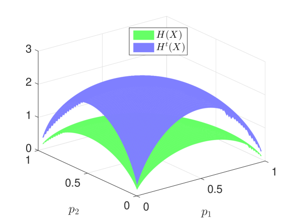
As its illustrated in Fig.1, the total entropy Ht(X)superscript𝐻𝑡𝑋H^{t}(X) shows more uncertainty beyond Shannon entropy.
Refer to caption
Figure 1: (Color online). A comparison of the Shannon entropy H(X)𝐻𝑋H(X) and total entropy Ht(X)superscript𝐻𝑡𝑋H^{t}(X) with respect to the probability distribution {pi}subscript𝑝𝑖\{p_{i}\}.

In quantum scenarios, inspired by the von Neumann entropy we can define the quantum total entropy for a given quantum state.

Definition 1

The total entropy of a quantum state ρ𝜌\rho on d𝑑d-dimensional Hilbert space {\cal H} is defined by

St(ρ)=Tr[ρlog2ρ+(𝟙ρ)log2(𝟙ρ)],superscript𝑆𝑡𝜌Trdelimited-[]𝜌subscript2𝜌1𝜌subscript21𝜌\displaystyle S^{t}(\rho)=-{\rm{Tr}}[\rho\log_{2}\rho+(\mathbbm{1}-\rho)\log_{2}(\mathbbm{1}-\rho)], (10)

where 𝟙1\mathbbm{1} is the identity matrix.

For a given state ρ𝜌\rho, the spectrum decomposition is given by ρ=iλi|ψiψi|𝜌subscript𝑖subscript𝜆𝑖ketsubscript𝜓𝑖brasubscript𝜓𝑖\rho=\sum_{i}\lambda_{i}|\psi_{i}\rangle\langle\psi_{i}|, where λisubscript𝜆𝑖\lambda_{i} are eigenvalues associated the orthogonal eigenvectors |ψiketsubscript𝜓𝑖|\psi_{i}\rangle. With this decomposition the Stsuperscript𝑆𝑡S^{t}-entropy is rewritten into

St(ρ)=i=1d(λilog2λi+(1λi)log2(1λi)).superscript𝑆𝑡𝜌subscriptsuperscript𝑑𝑖1subscript𝜆𝑖subscript2subscript𝜆𝑖1subscript𝜆𝑖subscript21subscript𝜆𝑖\displaystyle S^{t}(\rho)=-\sum^{d}_{i=1}(\lambda_{i}\log_{2}\lambda_{i}+(1-\lambda_{i})\log_{2}(1-\lambda_{i})). (11)

This states that the Stsuperscript𝑆𝑡S^{t}-entropy of a density matrix ρ𝜌\rho is equal to the classical Stsuperscript𝑆𝑡S^{t}-entropy of the probability distribution λ=(λ1,λ2,,λd)𝜆subscript𝜆1subscript𝜆2subscript𝜆𝑑\vec{\lambda}=(\lambda_{1},\lambda_{2},\cdots,\lambda_{d}) from the its eigenvalues.

Example 2. Consider a 555-qubit Heisenberg model with a random magnetic field in the z𝑧z-direction. Its Hamiltonian is given by

H5subscript𝐻5\displaystyle H_{5} =\displaystyle= 0.5σ1σ4+0.4σ2σ3+0.3σ3σ40.5subscript𝜎1subscript𝜎40.4subscript𝜎2subscript𝜎30.3subscript𝜎3subscript𝜎4\displaystyle 0.5\vec{\sigma}_{1}\cdot{}\vec{\sigma}_{4}+0.4\vec{\sigma}_{2}\cdot{}\vec{\sigma}_{3}+0.3\vec{\sigma}_{3}\cdot{}\vec{\sigma}_{4} (12)
0.5σ4σ5+i=15hjσjz,0.5subscript𝜎4subscript𝜎5superscriptsubscript𝑖15subscript𝑗superscriptsubscript𝜎𝑗𝑧\displaystyle-0.5\vec{\sigma}_{4}\cdot{}\vec{\sigma}_{5}+\sum_{i=1}^{5}h_{j}\sigma_{j}^{z},

where we suppose that the pairs of (1,3),(2,3),(3,4),(4,5)13233445(1,3),(2,3),(3,4),(4,5) are correlated each other, herein, σj=(σjx,σjy,σjz)subscript𝜎𝑗subscriptsuperscript𝜎𝑥𝑗subscriptsuperscript𝜎𝑦𝑗subscriptsuperscript𝜎𝑧𝑗\vec{\sigma}_{j}=(\sigma^{x}_{j},\sigma^{y}_{j},\sigma^{z}_{j}) represents a vector of Pauli matrices on qubit j𝑗j, hj[1,1]subscript𝑗11h_{j}\in[-1,1] denotes the strength of the disorder. For a 6-qubit system, the Hamiltonian is given by

H6subscript𝐻6\displaystyle H_{6} =\displaystyle= 0.4σ1σ3+0.5σ2σ50.3σ3σ40.4subscript𝜎1subscript𝜎30.5subscript𝜎2subscript𝜎50.3subscript𝜎3subscript𝜎4\displaystyle 0.4\vec{\sigma}_{1}\cdot{}\vec{\sigma}_{3}+0.5\vec{\sigma}_{2}\cdot{}\vec{\sigma}_{5}-0.3\vec{\sigma}_{3}\cdot{}\vec{\sigma}_{4} (13)
+0.2σ3σ6+0.6σ5σ6+i=16hjσjz,0.2subscript𝜎3subscript𝜎60.6subscript𝜎5subscript𝜎6superscriptsubscript𝑖16subscript𝑗superscriptsubscript𝜎𝑗𝑧\displaystyle+0.2\vec{\sigma}_{3}\cdot{}\vec{\sigma}_{6}+0.6\vec{\sigma}_{5}\cdot{}\vec{\sigma}_{6}+\sum_{i=1}^{6}h_{j}\sigma_{j}^{z},

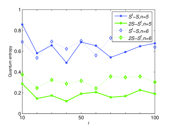
where the pairs of (1,3),(2,5),(3,4),(3,6),(5,6)1325343656(1,3),(2,5),(3,4),(3,6),(5,6) have correlation with each other. Consider the initial state |+5,|+6superscriptkettensor-productabsent5superscriptkettensor-productabsent6|+\rangle^{\otimes 5},|+\rangle^{\otimes 6} respectively, and the evolution time 100100100, where |+=12(|0+|1)ket12ket0ket1|+\rangle=\frac{1}{\sqrt{2}}(|0\rangle+|1\rangle). We can get the von Neumann entropy and the total Stsuperscript𝑆𝑡S^{t} entropy as shown in Fig.2.

Refer to caption
Figure 2: (Color online) A comparison of von Neumann entropy and the total Stsuperscript𝑆𝑡S^{t} entropy in terms of evolution time t𝑡t.

It follows that the von Neumann entropy is strictly smaller than the total Stsuperscript𝑆𝑡S^{t} entropy while the total Stsuperscript𝑆𝑡S^{t} entropy is no more than twice of von Neumann entropy, that is, SSt2S𝑆superscript𝑆𝑡2𝑆S\leq S^{t}\leq 2S.

Intuitively, the von Neumann entropy of a bipartite state |ΦABsubscriptketΦ𝐴𝐵|\Phi\rangle_{AB} on Hilbert space ABtensor-productsubscript𝐴subscript𝐵\mathcal{H}_{A}\otimes\mathcal{H}_{B} can be viewed as the uncertainty of an observer A𝐴A who can only access to the subsystem A𝐴A. While similar to classical scenarios, the present Stsuperscript𝑆𝑡S^{t}-entropy provides a method for describing its complementary dual information. In applications, one may suppose a mixed state represent an ensemble of pure states, that is, {pi,|ψi}subscript𝑝𝑖ketsubscript𝜓𝑖\{p_{i},|\psi_{i}\rangle\}. In this case, the density operator is defined by ρ=ipi|ψiψi|𝜌conditionalsubscript𝑖subscript𝑝𝑖subscript𝜓𝑖brasubscript𝜓𝑖\rho=\sum_{i}p_{i}|\psi_{i}\langle\psi_{i}|. Now, for each measurement outcome i𝑖i under the measurement operator Mi=|ψiψi|subscript𝑀𝑖ketsubscript𝜓𝑖brasubscript𝜓𝑖M_{i}=|\psi_{i}\rangle\langle\psi_{i}|, the quantum statistical probability is pi=Tr(Miρ)subscript𝑝𝑖Trsubscript𝑀𝑖𝜌p_{i}={\rm Tr}(M_{i}\rho). We can regard all the measurements except for Misubscript𝑀𝑖M_{i} as the complementary dual measurement of Misubscript𝑀𝑖M_{i}. This implies a positive-operator-value measurement (POVM) {Mi,IMi}subscript𝑀𝑖𝐼subscript𝑀𝑖\{M_{i},I-M_{i}\}, which follows the average information (5). Hence, the total entropy Stsuperscript𝑆𝑡S^{t} gives an extended extropy information obtained from quantum statistics beyond the von Neumann entropy.

For a quantum system described by a density operator ρ𝜌\rho, a general entropy function Canosa2002 may be defined as

Sf(ρ)=Trf(ρ)=if(λi),subscript𝑆𝑓𝜌Tr𝑓𝜌subscript𝑖𝑓subscript𝜆𝑖\displaystyle S_{f}(\rho)={\rm Tr}f(\rho)=\sum_{i}f(\lambda_{i}), (14)

where f𝑓f is a smooth concave function satisfying f(0)=f(1)=0𝑓0𝑓10f(0)=f(1)=0, λisubscript𝜆𝑖\lambda_{i} are the eigenvalues of ρ𝜌\rho. This includes the von Neumann entropy with

f(λ)=λlnλ.𝑓𝜆𝜆𝜆\displaystyle f(\lambda)=-\lambda\ln\lambda. (15)

While the Tsallis entropy Tsallis1988 may be defined according to

f(λ)=(λλq)q1,𝑓𝜆𝜆superscript𝜆𝑞𝑞1\displaystyle f(\lambda)=\frac{(\lambda-\lambda^{q})}{q-1}, (16)

where q>0𝑞0q>0 and q1𝑞1q\neq 1. Instead, the present Stsuperscript𝑆𝑡S^{t}-entropy (11) may be recovered according to

f(λ)=λlnλ(1λ)ln(1λ).𝑓𝜆𝜆𝜆1𝜆1𝜆\displaystyle f(\lambda)=-\lambda\ln\lambda-(1-\lambda)\ln(1-\lambda). (17)

This allows us construct one-parameter total entropy based on the Tsallis entropy and its complementary dual (see Appendix B).

Next, we show that the present Stsuperscript𝑆𝑡S^{t}-entropy satisfies the following properties.

Lemma 1

Let ρABsubscript𝜌𝐴𝐵\rho_{AB} be any density operator of a composite system AB𝐴𝐵AB, and ϱA(B)subscriptitalic-ϱ𝐴𝐵\varrho_{A(B)} be the reduced density operator of the subsystem A(B)𝐴𝐵A(B). The total entropy Stsuperscript𝑆𝑡S^{t} satisfies the following properties.

  • (i)

    Non-negativity: The total entropy satisfies 0St(ρ)dlog2d(d1)log2(d1)0superscript𝑆𝑡𝜌𝑑subscript2𝑑𝑑1subscript2𝑑10\leq S^{t}(\rho)\leq d\log_{2}d-(d-1)\log_{2}(d-1).

  • (ii)

    Concavity: For any convex combination ρ=i=1npiρi𝜌subscriptsuperscript𝑛𝑖1subscript𝑝𝑖subscript𝜌𝑖\rho=\sum^{n}_{i=1}p_{i}\rho_{i}, the total entropy satisfies

    i=1npiSt(ρi)St(ρ).subscriptsuperscript𝑛𝑖1subscript𝑝𝑖superscript𝑆𝑡subscript𝜌𝑖superscript𝑆𝑡𝜌\displaystyle\sum^{n}_{i=1}p_{i}S^{t}(\rho_{i})\leq S^{t}(\rho). (18)
  • (iii)

    Symmetry: For any pure state ρABsubscript𝜌𝐴𝐵\rho_{AB} the total entropy satisfies St(ϱA)=St(ϱB)superscript𝑆𝑡subscriptitalic-ϱ𝐴superscript𝑆𝑡subscriptitalic-ϱ𝐵S^{t}(\varrho_{A})=S^{t}(\varrho_{B}).

  • (iv)

    Invariance: The total entropy is invariant under any unitary transformation, that is, St(ρ)=St(UρU)superscript𝑆𝑡𝜌superscript𝑆𝑡𝑈𝜌superscript𝑈S^{t}(\rho)=S^{t}(U\rho U^{\dagger}) for any U𝕊𝕌(AB)𝑈𝕊𝕌tensor-productsubscript𝐴subscript𝐵U\in\mathbb{SU}({\cal H}_{A}\otimes{\cal H}_{B}).

  • (v)

    Subadditivity: For any product state ρ=ϱAϱB𝜌tensor-productsubscriptitalic-ϱ𝐴subscriptitalic-ϱ𝐵\rho=\varrho_{A}\otimes\varrho_{B}, the total entropy satisfies

    St(ρ)<St(ϱA)+St(ϱB)superscript𝑆𝑡𝜌superscript𝑆𝑡subscriptitalic-ϱ𝐴superscript𝑆𝑡subscriptitalic-ϱ𝐵\displaystyle S^{t}(\rho)<S^{t}(\varrho_{A})+S^{t}(\varrho_{B}) (19)

    and

    St(ρ)max{St(ϱA),St(ϱB)}.superscript𝑆𝑡𝜌superscript𝑆𝑡subscriptitalic-ϱ𝐴superscript𝑆𝑡subscriptitalic-ϱ𝐵\displaystyle S^{t}(\rho)\geq\max\{S^{t}(\varrho_{A}),S^{t}(\varrho_{B})\}. (20)
  • (vi)

    Boundedness: For any convex combination ρ=i=1npiρi𝜌subscriptsuperscript𝑛𝑖1subscript𝑝𝑖subscript𝜌𝑖\rho=\sum^{n}_{i=1}p_{i}\rho_{i}, the total entropy satisfies

    St(ρ)Ht(X),superscript𝑆𝑡𝜌superscript𝐻𝑡𝑋\displaystyle S^{t}(\rho)\leq H^{t}(X), (21)

    where X𝑋X is the classical random variable with distribution {p1,,pn}subscript𝑝1subscript𝑝𝑛\{p_{1},\cdots,p_{n}\}.

The proof of Lemma 1 is shown in Appendix A.

III The Stsuperscript𝑆𝑡S^{t}-entropy entanglement

Let 𝒮AB=𝒮(AB)superscript𝒮𝐴𝐵𝒮tensor-productsubscript𝐴subscript𝐵{\cal S}^{AB}={\cal S}(\mathcal{H}_{A}\otimes\mathcal{H}_{B}) be the set of density matrices acting on Hilbert space ABtensor-productsubscript𝐴subscript𝐵\mathcal{H}_{A}\otimes\mathcal{H}_{B}. A function E𝐸E: SAB+superscript𝑆𝐴𝐵subscriptS^{AB}\to{\mathbbm{R}}_{+} is called a measure of entanglement if it satisfies the following conditions entanglement2001 ; entanglement2009 :

  • (E1)

    E(ρ)=0𝐸𝜌0E(\rho)=0 if and only if ρ𝜌\rho is a separable state;

  • (E2)

    Invariance under local unitary transformations: E(ρ)=E((UAUB)ρ(UAUB))𝐸𝜌𝐸tensor-productsubscript𝑈𝐴subscript𝑈𝐵𝜌tensor-productsubscriptsuperscript𝑈𝐴subscriptsuperscript𝑈𝐵E(\rho)=E((U_{A}\otimes U_{B})\rho(U^{{\dagger}}_{A}\otimes U^{{\dagger}}_{B})) for any local unitary transformations UA𝕊𝕌(A),UB𝕊𝕌(B)formulae-sequencesubscript𝑈𝐴𝕊𝕌subscript𝐴subscript𝑈𝐵𝕊𝕌subscript𝐵U_{A}\in\mathbb{SU}(\mathcal{H}_{A}),U_{B}\in\mathbb{SU}(\mathcal{H}_{B});

  • (E3)

    Non-increasing on average under local operations and classical communication (LOCC) operations that is, jpjE(σj)E(ρ)subscript𝑗subscript𝑝𝑗𝐸subscript𝜎𝑗𝐸𝜌\sum_{j}p_{j}E(\sigma_{j})\leq E(\rho), where ΛLOCCsuperscriptΛ𝐿𝑂𝐶𝐶\Lambda^{LOCC} is an arbitrary LOCC operation defined by ΛLOCC(ρ)=jpjσjsuperscriptΛ𝐿𝑂𝐶𝐶𝜌subscript𝑗subscript𝑝𝑗subscript𝜎𝑗\Lambda^{LOCC}(\rho)=\sum_{j}p_{j}\sigma_{j}.

  • (E4)

    Convexity: E(ipiρi)ipiE(ρi)𝐸subscript𝑖subscript𝑝𝑖subscript𝜌𝑖subscript𝑖subscript𝑝𝑖𝐸subscript𝜌𝑖E(\sum_{i}p_{i}\rho_{i})\leq\sum_{i}p_{i}E(\rho_{i}) for any ρ=ipiρi𝜌subscript𝑖subscript𝑝𝑖subscript𝜌𝑖\rho=\sum_{i}p_{i}\rho_{i}, where {pi}subscript𝑝𝑖\{p_{i}\} is a probability distribution, and ρisubscript𝜌𝑖\rho_{i}’s are density matrices.

In what follows, we propose new bipartite entanglement measure named the Stsuperscript𝑆𝑡S^{t}-entropy entanglement from the total quantum entropy.

III.1 The Stsuperscript𝑆𝑡S^{t}-entropy entanglement

For a pure state |ΦABsubscriptketΦ𝐴𝐵|\Phi\rangle_{AB} on d×d𝑑𝑑d\times d dimensional Hilbert space ABtensor-productsubscript𝐴subscript𝐵{\cal H}_{A}\otimes{\cal H}_{B}, the Stsuperscript𝑆𝑡S^{t}-entropy entanglement is defined as

Et(|ΦAB)=1rSt(ϱA),subscript𝐸𝑡subscriptketΦ𝐴𝐵1𝑟superscript𝑆𝑡subscriptitalic-ϱ𝐴\displaystyle E_{t}(|\Phi\rangle_{AB})=\frac{1}{r}S^{t}(\varrho_{A}), (22)

where r=dlog2d(d1)log2(d1)𝑟𝑑subscript2𝑑𝑑1subscript2𝑑1r=d\log_{2}d-(d-1)\log_{2}(d-1) is a normalized factor and ϱA=TrB(|ΦABΦ|)subscriptitalic-ϱ𝐴subscriptTr𝐵subscriptketΦ𝐴𝐵braΦ\varrho_{A}={\rm Tr}_{B}(|\Phi\rangle_{AB}\langle\Phi|) denotes the reduced density operator of the subsystem A𝐴A.

For a bipartite mixed state ρABsubscript𝜌𝐴𝐵\rho_{AB} on Hilbert space ABtensor-productsubscript𝐴subscript𝐵{\cal H}_{A}\otimes{\cal H}_{B}, the Stsuperscript𝑆𝑡S^{t}-entropy entanglement is given via the convex-roof extension as

Et(ρAB)=inf{pi,|Φi}ipiEt(|ΦiAB),subscript𝐸𝑡subscript𝜌𝐴𝐵subscriptinfimumsubscript𝑝𝑖ketsubscriptΦ𝑖subscript𝑖subscript𝑝𝑖subscript𝐸𝑡subscriptketsubscriptΦ𝑖𝐴𝐵\displaystyle E_{t}(\rho_{AB})=\inf_{\{p_{i},|\Phi_{i}\rangle\}}\sum_{i}p_{i}E_{t}(|\Phi_{i}\rangle_{AB}), (23)

where Et(|ΦiAB)=St(ϱAi)subscript𝐸𝑡subscriptketsubscriptΦ𝑖𝐴𝐵superscript𝑆𝑡subscriptsuperscriptitalic-ϱ𝑖𝐴E_{t}(|\Phi_{i}\rangle_{AB})=S^{t}(\varrho^{i}_{A}) is the Stsuperscript𝑆𝑡S^{t}-entropy of the subsystem A𝐴A for the pure state ρABi=|ΦiABΦi|subscriptsuperscript𝜌𝑖𝐴𝐵subscriptketsubscriptΦ𝑖𝐴𝐵brasubscriptΦ𝑖\rho^{i}_{AB}=|\Phi_{i}\rangle_{AB}\langle\Phi_{i}|, and the infimum is taken over all the possible pure-state decompositions of ρAB=ipi|ΦiΦi|subscript𝜌𝐴𝐵subscript𝑖subscript𝑝𝑖ketsubscriptΦ𝑖brasubscriptΦ𝑖\rho_{AB}=\sum_{i}p_{i}|\Phi_{i}\rangle\langle\Phi_{i}| with pi0subscript𝑝𝑖0p_{i}\geq 0, ipi=1subscript𝑖subscript𝑝𝑖1\sum_{i}p_{i}=1. The quantity Et(ρ)subscript𝐸𝑡𝜌E_{t}(\rho) has defined an entanglement measure for any bipartite state.

Theorem 1

For an arbitrary finite-dimensional quantum state ρ𝜌\rho on Hilbert space ABtensor-productsubscript𝐴subscript𝐵{\cal H}_{A}\otimes{\cal H}_{B}, the quantity Etsubscript𝐸𝑡E_{t} is a bipartite entanglement measure.

Proof. For any density matrix ρ𝜌\rho on Hilbert space ABtensor-productsubscript𝐴subscript𝐵{\cal H}_{A}\otimes{\cal H}_{B}, it follows that Et(ρ)0subscript𝐸𝑡𝜌0E_{t}(\rho)\geq 0 from the non-negativity in Lemma 1 and Eq.(23), herein, the equality holds if and only if ρ𝜌\rho is separable. This has proved the condition (E1).

Note that the quantum Stsuperscript𝑆𝑡S^{t}-entropy is invariant under local unitary transformations from Lemma 1, this follows the condition (E2).

The concavity of Stsuperscript𝑆𝑡S^{t}-entropy in Lemma 1 assures the monotonicity under average local operations and classical communication (LOCC). Here, we firstly prove the monotonicity for pure states, i.e., when ρ𝜌\rho and σjsubscript𝜎𝑗\sigma_{j} are all pure states. From the definition of the quantum Stsuperscript𝑆𝑡S^{t}-entropy entanglement in Eq.(22), we have

Et(ρ)subscript𝐸𝑡𝜌\displaystyle E_{t}(\rho) =\displaystyle= St(ρA)superscript𝑆𝑡superscript𝜌𝐴\displaystyle S^{t}(\rho^{A}) (24)
=\displaystyle= St(jpjσjA)superscript𝑆𝑡subscript𝑗subscript𝑝𝑗subscriptsuperscript𝜎𝐴𝑗\displaystyle S^{t}(\sum_{j}p_{j}\sigma^{A}_{j})
\displaystyle\geq jpjSt(σjA)subscript𝑗subscript𝑝𝑗superscript𝑆𝑡subscriptsuperscript𝜎𝐴𝑗\displaystyle\sum_{j}p_{j}S^{t}(\sigma^{A}_{j})
=\displaystyle= jpjEt(σj),subscript𝑗subscript𝑝𝑗subscript𝐸𝑡subscript𝜎𝑗\displaystyle\sum_{j}p_{j}E_{t}(\sigma_{j}), (25)

where the inequality (24) is from the concavity of the quantum Stsuperscript𝑆𝑡S^{t}-entropy in Lemma 1. The definition of the Stsuperscript𝑆𝑡S^{t}-entropy entanglement in Eq.(22) implies Eq.(25). According to Ref.Vidal2000 , the monotonicity for mixed states can be inherited from the monotonicity of pure states via the convex roof extension. This has proved the condition (E3).

Finally, the convexity (E4) is followed directly from the fact that all the entanglement measures constructed via the convex roof extension are convex 3H2009 . \Box

III.2 Analytic formula for two-qubit states

In this subsection, we provide an analytic formula of the Stsuperscript𝑆𝑡S^{t}-entropy entanglement for two-qubit systems. For any bipartite pure state |ΦABsubscriptketΦ𝐴𝐵|\Phi\rangle_{AB} on Hilbert space ABtensor-productsubscript𝐴subscript𝐵{\cal H}_{A}\otimes{\cal H}_{B}, its concurrence is defined by Rungta2001 :

C(|ΦAB)=2(1Tr(ϱA2)),𝐶subscriptketΦ𝐴𝐵21Trsubscriptsuperscriptitalic-ϱ2𝐴\displaystyle C(|\Phi\rangle_{AB})=\sqrt{2(1-{\rm Tr}(\varrho^{2}_{A}))}, (26)

where ϱA=TrB(|ΦABΦ|)subscriptitalic-ϱ𝐴subscriptTr𝐵subscriptketΦ𝐴𝐵braΦ\varrho_{A}={\rm Tr}_{B}(|\Phi\rangle_{AB}\langle\Phi|) is the reduced density operator of the subsystem A𝐴A.

For a mixed state ρABsubscript𝜌𝐴𝐵\rho_{AB} on Hilbert space ABtensor-productsubscript𝐴subscript𝐵{\cal H}_{A}\otimes{\cal H}_{B}, the concurrence is given by the convex extension as

C(ρAB)=inf{pi,|Φi}ipiC(|ΦiAB),𝐶subscript𝜌𝐴𝐵subscriptinfimumsubscript𝑝𝑖ketsubscriptΦ𝑖subscript𝑖subscript𝑝𝑖𝐶subscriptketsubscriptΦ𝑖𝐴𝐵\displaystyle C(\rho_{AB})=\inf_{\{p_{i},|\Phi_{i}\rangle\}}\sum_{i}p_{i}C(|\Phi_{i}\rangle_{AB}), (27)

where the infimum takes over all the possible pure-state decompositions of ρABsubscript𝜌𝐴𝐵\rho_{AB}, i.e., ρAB=ipi|ΦiABΦi|subscript𝜌𝐴𝐵subscript𝑖subscript𝑝𝑖subscriptketsubscriptΦ𝑖𝐴𝐵brasubscriptΦ𝑖\rho_{AB}=\sum_{i}p_{i}|\Phi_{i}\rangle_{AB}\langle\Phi_{i}|, {pi}subscript𝑝𝑖\{p_{i}\} is a probability distribution with pi0subscript𝑝𝑖0p_{i}\geq 0 and ipi=1subscript𝑖subscript𝑝𝑖1\sum_{i}p_{i}=1.

Interestingly, for a two-qubit mixed state ρ𝜌\rho on Hilbert space ABtensor-productsubscript𝐴subscript𝐵{\cal H}_{A}\otimes{\cal H}_{B}, its concurrence has the analytic formula as follows Coffman2000 :

C(ρ)=max{0,λ1λ2λ3λ4},𝐶𝜌0subscript𝜆1subscript𝜆2subscript𝜆3subscript𝜆4\displaystyle C(\rho)=\max\{0,\lambda_{1}-\lambda_{2}-\lambda_{3}-\lambda_{4}\}, (28)

with λisubscript𝜆𝑖\lambda_{i}’s being eigenvalues of the matrix ρ(σYσY)ρ(σYσY)𝜌tensor-productsubscript𝜎𝑌subscript𝜎𝑌superscript𝜌tensor-productsubscript𝜎𝑌subscript𝜎𝑌\sqrt{\rho(\sigma_{Y}\otimes\sigma_{Y})\rho^{*}(\sigma_{Y}\otimes\sigma_{Y})} in decreasing order, herein, ρsuperscript𝜌\rho^{*} is the complex conjugate of ρ𝜌\rho, and σYsubscript𝜎𝑌\sigma_{Y} denotes Pauli operator.

Now, consider any 𝒞2𝒞dtensor-productsuperscript𝒞2superscript𝒞𝑑{\cal C}^{2}\otimes{\cal C}^{d} pure state |ϕABsubscriptketitalic-ϕ𝐴𝐵|\phi\rangle_{AB} on Hilbert space ABtensor-productsubscript𝐴subscript𝐵\mathcal{H}_{A}\otimes\mathcal{H}_{B} with Schmidt decomposition

|ϕAB=λ0|0|ϕ0+λ1|1|ϕ1,subscriptketitalic-ϕ𝐴𝐵subscript𝜆0ket0ketsubscriptitalic-ϕ0subscript𝜆1ket1ketsubscriptitalic-ϕ1\displaystyle|\phi\rangle_{AB}=\sqrt{\lambda_{0}}|0\rangle|\phi_{0}\rangle+\sqrt{\lambda_{1}}|1\rangle|\phi_{1}\rangle, (29)

where the subsystem A𝐴A is qubit while the subsystem B𝐵B is on finite dimensional space, and {|ϕi}ketsubscriptitalic-ϕ𝑖\{|\phi_{i}\rangle\} are orthogonal states on Bsubscript𝐵\mathcal{H}_{B}. From Eq.(22), we get the Stsuperscript𝑆𝑡S^{t}-entropy entanglement as

Et(|ϕAB)=λ0log2λ0λ1log2λ1.subscript𝐸𝑡subscriptketitalic-ϕ𝐴𝐵subscript𝜆0subscript2subscript𝜆0subscript𝜆1subscript2subscript𝜆1\displaystyle E_{t}(|\phi\rangle_{AB})=-\lambda_{0}\log_{2}\lambda_{0}-\lambda_{1}\log_{2}\lambda_{1}. (30)

Besides, the concurrence of |ΨABsubscriptketΨ𝐴𝐵|\Psi\rangle_{AB} is given by

C(|ϕAB)=2(1Tr(ϱA2))=2λ0λ1.𝐶subscriptketitalic-ϕ𝐴𝐵21Trsubscriptsuperscriptitalic-ϱ2𝐴2subscript𝜆0subscript𝜆1\displaystyle C(|\phi\rangle_{AB})=\sqrt{2(1-{\rm{Tr}}(\varrho^{2}_{A}))}=2\sqrt{\lambda_{0}\lambda_{1}}. (31)

This can be proved that

Et(|ϕAB)=h(C(|ϕAB)),subscript𝐸𝑡subscriptketitalic-ϕ𝐴𝐵𝐶subscriptketitalic-ϕ𝐴𝐵\displaystyle E_{t}(|\phi\rangle_{AB})=h(C(|\phi\rangle_{AB})), (32)

where h(x)𝑥h(x) is an analytic function defined as

h(x)𝑥\displaystyle h(x) =\displaystyle= 1+1x22log21+1x2211superscript𝑥22subscript211superscript𝑥22\displaystyle-\frac{1+\sqrt{1-x^{2}}}{2}\log_{2}\frac{1+\sqrt{1-x^{2}}}{2} (33)
11x22log2(11x22).11superscript𝑥22subscript211superscript𝑥22\displaystyle-\frac{1-\sqrt{1-x^{2}}}{2}\log_{2}(\frac{1-\sqrt{1-x^{2}}}{2}).

Thus, we get a functional relation (32) between the concurrence and Stsuperscript𝑆𝑡S^{t}-entropy entanglement for any qubit-qudit pure state on Hilbert space ABtensor-productsubscript𝐴subscript𝐵\mathcal{H}_{A}\otimes\mathcal{H}_{B}.

In fact, for any two-qubit mixed state, the Stsuperscript𝑆𝑡S^{t}-entropy entanglement has a similar relation with Eq.(32). Here, we firstly prove the monotonicity and convexity of h(x)𝑥h(x) in Eq.(33).

Proposition 1

The function h(x)𝑥h(x) defined in Eq.(33) is monotonically increasing and convex.

Proof. Since h(x)𝑥h(x) is an analytic function on x(0,1)𝑥01x\in(0,1), its monotonicity and convexity can be followed from the nonnegativity of its first and second derivatives. In fact, the first derivative of h(x)𝑥h(x) is given by

dh(x)dx=x21x2×log21+1x211x2.𝑑𝑥𝑑𝑥𝑥21superscript𝑥2subscript211superscript𝑥211superscript𝑥2\displaystyle\frac{dh(x)}{dx}=\frac{x}{2\sqrt{1-x^{2}}}\times\log_{2}\frac{1+\sqrt{1-x^{2}}}{1-\sqrt{1-x^{2}}}. (34)

This is always nonnegative on x[0,1]𝑥01x\in[0,1]. Moreover, we can get Eq. (34) is positive for x(0,1)𝑥01x\in(0,1). This means that h(x)𝑥h(x) is a strictly monotone increasing function on x[0,1]𝑥01x\in[0,1]. While, from Eq.(34) the second derivative of h(x)𝑥h(x) is given by

d2h(x)dx2=21x2+ln(1+1x2)ln(11x2)2ln2×(1x2)3.superscript𝑑2𝑥𝑑superscript𝑥221superscript𝑥211superscript𝑥211superscript𝑥222superscript1superscript𝑥23\displaystyle\frac{d^{2}h(x)}{dx^{2}}=\frac{-2\sqrt{1-x^{2}}+\ln(1+\sqrt{1-x^{2}})-\ln(1-\sqrt{1-x^{2}})}{2\ln 2\times\sqrt{(1-x^{2})^{3}}}. (35)

which is positive for any x(0,1)𝑥01x\in(0,1).

For any given two-qubit mixed state ρ𝜌\rho there is an optimal pure-state decomposition ρAB=ipi|ΦiABΦi|subscript𝜌𝐴𝐵subscript𝑖subscript𝑝𝑖subscriptketsubscriptΦ𝑖𝐴𝐵brasubscriptΦ𝑖\rho_{AB}=\sum_{i}p_{i}|\Phi_{i}\rangle_{AB}\langle\Phi_{i}| such that its concurrence is equal to its average pure-state concurrences Wootters1998 , that is, we get

C(ρAB)=ipiC(|ΦiAB)𝐶subscript𝜌𝐴𝐵subscript𝑖subscript𝑝𝑖𝐶subscriptketsubscriptΦ𝑖𝐴𝐵\displaystyle C(\rho_{AB})=\sum_{i}p_{i}C(|\Phi_{i}\rangle_{AB}) (36)

This means that

h(C(ρAB))𝐶subscript𝜌𝐴𝐵\displaystyle h(C(\rho_{AB})) =\displaystyle= h(ipiC(|ΨiAB))subscript𝑖subscript𝑝𝑖𝐶subscriptketsubscriptΨ𝑖𝐴𝐵\displaystyle h(\sum_{i}p_{i}C(|\Psi_{i}\rangle_{AB})) (37)
=\displaystyle= ipih(C(|ΨiAB))subscript𝑖subscript𝑝𝑖𝐶subscriptketsubscriptΨ𝑖𝐴𝐵\displaystyle\sum_{i}p_{i}h(C(|\Psi_{i}\rangle_{AB}))
=\displaystyle= ipiEt(|ΨiAB)subscript𝑖subscript𝑝𝑖subscript𝐸𝑡subscriptketsubscriptΨ𝑖𝐴𝐵\displaystyle\sum_{i}p_{i}E_{t}(|\Psi_{i}\rangle_{AB}) (38)
\displaystyle\geq Et(ρAB),subscript𝐸𝑡subscript𝜌𝐴𝐵\displaystyle E_{t}(\rho_{AB}), (39)

where the equality (37) is followed from Eq.(36), the equality (38) is obtained by using Eq.(32), and the inequality (39) is due to the definition of Et(ρAB)subscript𝐸𝑡subscript𝜌𝐴𝐵E_{t}(\rho_{AB}) in Eq.(23).

Moreover, from the optimal decomposition of ρAB=jpj|ujuj|subscript𝜌𝐴𝐵subscript𝑗subscript𝑝𝑗ketsubscript𝑢𝑗brasubscript𝑢𝑗\rho_{AB}=\sum_{j}p_{j}|u_{j}\rangle\langle u_{j}| for the Stsuperscript𝑆𝑡S^{t}-entropy entanglement we get that

Et(ρAB)subscript𝐸𝑡subscript𝜌𝐴𝐵\displaystyle E_{t}(\rho_{AB}) =\displaystyle= jpjEt(|ujAB))\displaystyle\sum_{j}p_{j}E_{t}(|u_{j}\rangle_{AB})) (40)
=\displaystyle= jpjh(C(|ujAB))subscript𝑗subscript𝑝𝑗𝐶subscriptketsubscript𝑢𝑗𝐴𝐵\displaystyle\sum_{j}p_{j}h(C(|u_{j}\rangle_{AB}))
\displaystyle\geq h(jpjC(|ujAB))subscript𝑗subscript𝑝𝑗𝐶subscriptketsubscript𝑢𝑗𝐴𝐵\displaystyle h(\sum_{j}p_{j}C(|u_{j}\rangle_{AB})) (41)
\displaystyle\geq h(C(ρAB)),𝐶subscript𝜌𝐴𝐵\displaystyle h(C(\rho_{AB})), (42)

where the equality (40) is followed from the relation (32), the inequality (41) is derived from the convexity of h(x)𝑥h(x) in Proposition 1, and the inequality (42) is from the monotonicity of h(x)𝑥h(x) and the definition of C(ρAB)𝐶subscript𝜌𝐴𝐵C(\rho_{AB}) in Eq.(27).

Combing Eqs.(39) with (42), we have

Et(ρAB)=h(C(ρAB))subscript𝐸𝑡subscript𝜌𝐴𝐵𝐶subscript𝜌𝐴𝐵\displaystyle E_{t}(\rho_{AB})=h(C(\rho_{AB})) (43)

for any two-qubit mixed state ρABsubscript𝜌𝐴𝐵\rho_{AB}. So, Eq.(43) provides an analytic formula of the Stsuperscript𝑆𝑡S^{t}-entropy entanglement for any two-qubit state.

IV Monogamy inequality of the Stsuperscript𝑆𝑡S^{t}-entropy entanglement in multi-dimensional systems

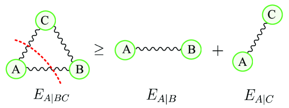
The original monogamy of the entanglement is quantitatively shown in the inequality (2). For a tripartite system, its monogamy relation is shown in Fig.3. However, the inequality (2) may be invalid for general entanglement measures. Thus a natural question is to determine whether a given entanglement measure is monogamous or not.
Refer to caption
Figure 3: (Color online). A monogamy relation for tripartite systems A𝐴A, B𝐵B, and C𝐶C in terms of the entanglement measure E𝐸E. Green circles represent the parties, wavy lines represent entangled sources, the red dotted curve represents the bipartition.

IV.1 The n𝑛n-qubit systems

The Stsuperscript𝑆𝑡S^{t}-entropy entanglement for qubit systems can be reduced to the entanglement of formation (EOF) corresponding to the case of d=2𝑑2d=2 in Eq.(30). In fact, for a pure state |ΦABsubscriptketΦ𝐴𝐵|\Phi\rangle_{AB} on Hilbert space ABtensor-productsubscript𝐴subscript𝐵{\cal H}_{A}\otimes{\cal H}_{B}, EOF is defined via the non Neumann entropy as Bennett19963824 ; Wootters1998 :

Ef(|ΦAB)=S(ϱA)=Tr(ϱAlog2ϱA),subscript𝐸𝑓subscriptketΦ𝐴𝐵𝑆subscriptitalic-ϱ𝐴Trsubscriptitalic-ϱ𝐴subscript2subscriptitalic-ϱ𝐴\displaystyle E_{f}(|\Phi\rangle_{AB})=S(\varrho_{A})=-{\rm{Tr}}(\varrho_{A}\log_{2}\varrho_{A}), (44)

where ϱA=TrB(|ΦABΦ|)subscriptitalic-ϱ𝐴subscriptTr𝐵subscriptketΦ𝐴𝐵braΦ\varrho_{A}={\rm Tr}_{B}(|\Phi\rangle_{AB}\langle\Phi|) denotes the reduced density operator of the subsystem A𝐴A. EOF for a bipartite mixed state ρABsubscript𝜌𝐴𝐵\rho_{AB} on Hilbert space ABtensor-productsubscript𝐴subscript𝐵{\cal H}_{A}\otimes{\cal H}_{B} is given by

Ef(ρAB)=inf{pi,|Φi}ipiE(|Φi)AB,subscript𝐸𝑓subscript𝜌𝐴𝐵subscriptinfimumsubscript𝑝𝑖ketsubscriptΦ𝑖subscript𝑖subscript𝑝𝑖𝐸subscriptketsubscriptΦ𝑖𝐴𝐵\displaystyle E_{f}(\rho_{AB})=\inf_{\{p_{i},|\Phi_{i}\rangle\}}\sum_{i}p_{i}E(|\Phi_{i}\rangle)_{AB}, (45)

where the infimum takes over all the possible pure-state decompositions of ρAB=ipi|ΦiABΦi|subscript𝜌𝐴𝐵subscript𝑖subscript𝑝𝑖subscriptketsubscriptΦ𝑖𝐴𝐵brasubscriptΦ𝑖\rho_{AB}=\sum_{i}p_{i}|\Phi_{i}\rangle_{AB}\langle\Phi_{i}| and {pi}subscript𝑝𝑖\{p_{i}\} is a probability distribution. It has been proved that the squared EOF is monogamous for any n𝑛n-qubit system ρA1A2Ansubscript𝜌subscript𝐴1subscript𝐴2subscript𝐴𝑛\rho_{A_{1}A_{2}\cdots A_{n}} on Hilbert space i=1nAisuperscriptsubscripttensor-product𝑖1𝑛absentsubscriptsubscript𝐴𝑖\otimes_{i=1}^{n}\mathcal{H}_{A_{i}}, that is,

Ef2(ρA1|A2An)i=2nEf2(ρA1|Ai).subscriptsuperscript𝐸2𝑓subscript𝜌conditionalsubscript𝐴1subscript𝐴2subscript𝐴𝑛superscriptsubscript𝑖2𝑛subscriptsuperscript𝐸2𝑓subscript𝜌conditionalsubscript𝐴1subscript𝐴𝑖\displaystyle E^{2}_{f}(\rho_{A_{1}|A_{2}\cdots A_{n}})\geq\sum_{i=2}^{n}E^{2}_{f}(\rho_{A_{1}|A_{i}}). (46)

where E(ρA1|A2An)𝐸subscript𝜌conditionalsubscript𝐴1subscript𝐴2subscript𝐴𝑛E(\rho_{A_{1}|A_{2}\cdots A_{n}}) characterizes the bipartite entanglement with respect to the bipartition A1subscript𝐴1A_{1} and A2Ansubscript𝐴2subscript𝐴𝑛A_{2}\cdots A_{n}, and E(ρA1|Ai)𝐸subscript𝜌conditionalsubscript𝐴1subscript𝐴𝑖E(\rho_{A_{1}|A_{i}}) is the bipartite entanglement of the reduced density operator ρA1|Ai=TrA1Ai1Ai+1An(ρA1|A2An)subscript𝜌conditionalsubscript𝐴1subscript𝐴𝑖subscriptTrsubscript𝐴1subscript𝐴𝑖1subscript𝐴𝑖1subscript𝐴𝑛subscript𝜌conditionalsubscript𝐴1subscript𝐴2subscript𝐴𝑛\rho_{A_{1}|A_{i}}={\rm Tr}_{A_{1}\cdots A_{i-1}A_{i+1}\cdots A_{n}}(\rho_{A_{1}|A_{2}\cdots A_{n}}) of joint subsystems A1subscript𝐴1A_{1} and Aisubscript𝐴𝑖A_{i} for i=2,,n𝑖2𝑛i=2,\cdots,n.

From Eqs.(32) and (43), there exists the same analytic formula of the Stsuperscript𝑆𝑡S^{t}-entropy entanglement and EOF for any qubit system. Combined with the monogamy properties of EOF Bai3 ; Bai2014 ; Zhu2014 , we can prove that the squared Stsuperscript𝑆𝑡S^{t}-entropy entanglement is monogamous for any n𝑛n-qubit system ρA1A2Ansubscript𝜌subscript𝐴1subscript𝐴2subscript𝐴𝑛\rho_{A_{1}A_{2}\cdots A_{n}} on Hilbert space i=1nAisuperscriptsubscripttensor-product𝑖1𝑛absentsubscriptsubscript𝐴𝑖\otimes_{i=1}^{n}\mathcal{H}_{A_{i}}, that is,

Et2(ρA1|A2An)i=2nEt2(ρA1|Ai).subscriptsuperscript𝐸2𝑡subscript𝜌conditionalsubscript𝐴1subscript𝐴2subscript𝐴𝑛superscriptsubscript𝑖2𝑛subscriptsuperscript𝐸2𝑡subscript𝜌conditionalsubscript𝐴1subscript𝐴𝑖\displaystyle E^{2}_{t}(\rho_{A_{1}|A_{2}\cdots A_{n}})\geq\sum_{i=2}^{n}E^{2}_{t}(\rho_{A_{1}|A_{i}}). (47)

This means that both the EOF and Stsuperscript𝑆𝑡S^{t}-entropy entanglement have the same monogamy features.

IV.2 High dimensional systems

Our goal in this subsection is to extend the monogamy relationship for high dimensional systems. This will be explained by using several higher-dimensional states.

Consider a multipartite quantum system |ΨketΨ|\Psi\rangle on Hilbert space i=1nAisuperscriptsubscripttensor-product𝑖1𝑛absentsubscriptsubscript𝐴𝑖\otimes_{i=1}^{n}\mathcal{H}_{A_{i}}. Define the “residual entanglement” of the Stsuperscript𝑆𝑡S^{t}-entropy entanglement as

τγEt(|ΨA1A2An)=Etγ(|ΨA1|A2An)i=2nEtγ(ρA1|Ai),superscriptsubscript𝜏𝛾subscript𝐸𝑡subscriptketΨsubscript𝐴1subscript𝐴2subscript𝐴𝑛superscriptsubscript𝐸𝑡𝛾subscriptketΨconditionalsubscript𝐴1subscript𝐴2subscript𝐴𝑛subscriptsuperscript𝑛𝑖2superscriptsubscript𝐸𝑡𝛾subscript𝜌conditionalsubscript𝐴1subscript𝐴𝑖\displaystyle\tau_{\gamma}^{E_{t}}(|\Psi\rangle_{A_{1}A_{2}\cdots A_{n}})=E_{t}^{\gamma}(|\Psi\rangle_{A_{1}|A_{2}\cdots A_{n}})-\sum^{n}_{i=2}E_{t}^{\gamma}(\rho_{A_{1}|A_{i}}), (48)

where Et(|ΨA1|A2An)subscript𝐸𝑡subscriptketΨconditionalsubscript𝐴1subscript𝐴2subscript𝐴𝑛E_{t}(|\Psi\rangle_{A_{1}|A_{2}\cdots A_{n}}) denotes the bipartite entanglement with respect to the bipartition A1subscript𝐴1A_{1} and A2Ansubscript𝐴2subscript𝐴𝑛A_{2}\cdots A_{n}, and Et(ρA1|Ai)subscript𝐸𝑡subscript𝜌conditionalsubscript𝐴1subscript𝐴𝑖E_{t}(\rho_{A_{1}|A_{i}}) is the bipartite entanglement of the reduced density operator ρA1|Aisubscript𝜌conditionalsubscript𝐴1subscript𝐴𝑖\rho_{A_{1}|A_{i}} of joint subsystems A1subscript𝐴1A_{1} and Aisubscript𝐴𝑖A_{i} for i=2,,n𝑖2𝑛i=2,\cdots,n, and γ𝛾\gamma is a parameter with γ(0,)𝛾0\gamma\in(0,\infty). We show that the Stsuperscript𝑆𝑡S^{t}-entropy entanglement has different monogamy relationship from EOF.

Proposition 2

The monogamy of Stsuperscript𝑆𝑡S^{t}-entropy entanglement and EOF are inequivalent for high dimensional entangled systems.

Proposition 2 is proved by using the following examples.

Example 3. Consider a 422tensor-product4224\otimes 2\otimes 2 system Luo2022 in the pure state |ΨABCsubscriptketΨ𝐴𝐵𝐶|\Psi\rangle_{ABC} given by

|ΨABC=12(α|000+β|110+α|201+β|311),subscriptketΨ𝐴𝐵𝐶12𝛼ket000𝛽ket110𝛼ket201𝛽ket311\displaystyle|\Psi\rangle_{ABC}=\frac{1}{\sqrt{2}}(\alpha|000\rangle+\beta|110\rangle+\alpha|201\rangle+\beta|311\rangle), (49)

where α𝛼\alpha and β𝛽\beta satisfies that α2+β2=1superscript𝛼2superscript𝛽21\alpha^{2}+\beta^{2}=1. The reduced density operator of the subsystem A𝐴A is given by

ϱAsubscriptitalic-ϱ𝐴\displaystyle\varrho_{A} =\displaystyle= α22|0000|+β22|0101|.superscript𝛼22ket00quantum-operator-product00superscript𝛽2201bra01\displaystyle\frac{\alpha^{2}}{2}|00\rangle\langle 00|+\frac{\beta^{2}}{2}|01\rangle\langle 01|. (50)
+α22|1010|+β22|1111|.superscript𝛼22ket10quantum-operator-product10superscript𝛽2211bra11\displaystyle+\frac{\alpha^{2}}{2}|10\rangle\langle 10|+\frac{\beta^{2}}{2}|11\rangle\langle 11|.

From Eq.(22) we get

Et(|ΨA|BC)=a+b+483log23,subscript𝐸𝑡subscriptketΨconditional𝐴𝐵𝐶𝑎𝑏483subscript23\displaystyle E_{t}(|\Psi\rangle_{A|BC})=\frac{a+b+4}{8-3\log_{2}3}, (51)

where a=α2log2α2(2α2)log2(2α2)𝑎superscript𝛼2subscript2superscript𝛼22superscript𝛼2subscript22superscript𝛼2a=-\alpha^{2}\log_{2}\alpha^{2}-(2-\alpha^{2})\log_{2}(2-\alpha^{2}) and b=β2log2β2(2β2)log2(2β2)𝑏superscript𝛽2subscript2superscript𝛽22superscript𝛽2subscript22superscript𝛽2b=-\beta^{2}\log_{2}\beta^{2}-(2-\beta^{2})\log_{2}(2-\beta^{2}). The reduced state for the joint system A𝐴A and B𝐵B is given by

ρAB=12(|ψ1ψ1|+|ψ2ψ2|),subscript𝜌𝐴𝐵12ketsubscript𝜓1brasubscript𝜓1ketsubscript𝜓2brasubscript𝜓2\displaystyle\rho_{AB}=\frac{1}{2}(|\psi_{1}\rangle\langle\psi_{1}|+|\psi_{2}\rangle\langle\psi_{2}|), (52)

where |ϕiketsubscriptitalic-ϕ𝑖|\phi_{i}\rangle are defined by |ψ1=α|00+β|11)|\psi_{1}\rangle=\alpha|00\rangle+\beta|11\rangle) and |ψ2=α|20+β|31ketsubscript𝜓2𝛼ket20𝛽ket31|\psi_{2}\rangle=\alpha|20\rangle+\beta|31\rangle. For any pure state decomposition of ρABsubscript𝜌𝐴𝐵\rho_{AB}, the pure state component has the form

|μi=ai|ψ1+eiδ1ai2|ψ2,ketsubscript𝜇𝑖subscript𝑎𝑖ketsubscript𝜓1superscript𝑒𝑖𝛿1subscriptsuperscript𝑎2𝑖ketsubscript𝜓2\displaystyle|\mu_{i}\rangle=a_{i}|\psi_{1}\rangle+e^{-i\delta}\sqrt{1-a^{2}_{i}}|\psi_{2}\rangle, (53)

In this case, the reduced density operator is given by ϱBi=α2|00|+β2|11|subscriptsuperscriptitalic-ϱ𝑖𝐵superscript𝛼2ket0quantum-operator-product0superscript𝛽21bra1\varrho^{i}_{B}=\alpha^{2}|0\rangle\langle 0|+\beta^{2}|1\rangle\langle 1|. Therefore, according to the definition of the Stsuperscript𝑆𝑡S^{t}-entropy entanglement in Eq.(23), we have

Et(ρAB)=2α2log2α22β2log2β283log23.subscript𝐸𝑡subscript𝜌𝐴𝐵2superscript𝛼2subscript2superscript𝛼22superscript𝛽2subscript2superscript𝛽283subscript23\displaystyle E_{t}(\rho_{AB})=\frac{-2\alpha^{2}\log_{2}\alpha^{2}-2\beta^{2}\log_{2}\beta^{2}}{8-3\log_{2}3}. (54)

In a similar manner, for the reduced quantum state ρACsubscript𝜌𝐴𝐶\rho_{AC}, the reduced density operator is given by ϱCi=12|00|+12|11|subscriptsuperscriptitalic-ϱ𝑖𝐶12ket0quantum-operator-product0121bra1\varrho^{i}_{C}=\frac{1}{2}|0\rangle\langle 0|+\frac{1}{2}|1\rangle\langle 1|. This implies that

Et(ρAC)=283log23.subscript𝐸𝑡subscript𝜌𝐴𝐶283subscript23\displaystyle E_{t}(\rho_{AC})=\frac{2}{8-3\log_{2}3}. (55)

So, the “residual tangle” of the Stsuperscript𝑆𝑡S^{t}-entropy entanglement is given by

τEt(|ΨA|BC)=Et(|ΨA|BC)Et(ρAB)Et(ρAC)0superscript𝜏subscript𝐸𝑡subscriptketΨconditional𝐴𝐵𝐶subscript𝐸𝑡subscriptketΨconditional𝐴𝐵𝐶subscript𝐸𝑡subscript𝜌𝐴𝐵subscript𝐸𝑡subscript𝜌𝐴𝐶0\displaystyle\tau^{E_{t}}(|\Psi\rangle_{A|BC})=E_{t}(|\Psi\rangle_{A|BC})-E_{t}(\rho_{AB})-E_{t}(\rho_{AC})\not=0 (56)

for γ=1𝛾1\gamma=1. Instead, the “residual tangle” of the EOF entanglement is given by Bai2014 :

Ef(|ΨA|BC)=α2log2α2β2log2β2+1subscript𝐸𝑓subscriptketΨconditional𝐴𝐵𝐶superscript𝛼2subscript2superscript𝛼2superscript𝛽2subscript2superscript𝛽21\displaystyle E_{f}(|\Psi\rangle_{A|BC})=-\alpha^{2}\log_{2}\alpha^{2}-\beta^{2}\log_{2}\beta^{2}+1 (57)
Ef(ρAB)=α2log2α2β2log2β2subscript𝐸𝑓subscript𝜌𝐴𝐵superscript𝛼2subscript2superscript𝛼2superscript𝛽2subscript2superscript𝛽2\displaystyle E_{f}(\rho_{AB})=-\alpha^{2}\log_{2}\alpha^{2}-\beta^{2}\log_{2}\beta^{2} (58)
Ef(ρAC)=1subscript𝐸𝑓subscript𝜌𝐴𝐶1\displaystyle E_{f}(\rho_{AC})=1 (59)

which follows

τγEf(|ΨA|BC)=Efγ(|ΨA|BC)Efγ(ρAB)Efγ(ρAC)=0superscriptsubscript𝜏𝛾subscript𝐸𝑓subscriptketΨconditional𝐴𝐵𝐶superscriptsubscript𝐸𝑓𝛾subscriptketΨconditional𝐴𝐵𝐶superscriptsubscript𝐸𝑓𝛾subscript𝜌𝐴𝐵superscriptsubscript𝐸𝑓𝛾subscript𝜌𝐴𝐶0\displaystyle\tau_{\gamma}^{E_{f}}(|\Psi\rangle_{A|BC})=E_{f}^{\gamma}(|\Psi\rangle_{A|BC})-E_{f}^{\gamma}(\rho_{AB})-E_{f}^{\gamma}(\rho_{AC})=0 (60)

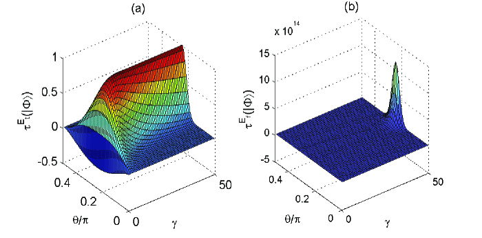
for γ=1𝛾1\gamma=1. For general γ1𝛾1\gamma\not=1, both residual tangles are shown Fig.4. We obtain the residual tangle of τEtsuperscript𝜏subscript𝐸𝑡\tau^{E_{t}} is negative while τEfsuperscript𝜏subscript𝐸𝑓\tau^{E_{f}} is zero.

Refer to caption
Figure 4: (Color online). The indicator τ𝜏\tau for a 422tensor-product4224\otimes 2\otimes 2 dimensional entanglement in Example 3. (a) The Stsuperscript𝑆𝑡S^{t}-entropy entanglement. (b) The EOF entanglement. Here, α=cosθ𝛼𝜃\alpha=\cos\theta and β=sinθ𝛽𝜃\beta=\sin\theta. τEtsuperscript𝜏subscript𝐸𝑡\tau^{E_{t}} is defined in Eq.(56) while τEfsuperscript𝜏subscript𝐸𝑓\tau^{E_{f}} is defined in Eq.(60).

Example 4. Consider a 633tensor-product6336\otimes 3\otimes 3 dimensional system in the pure state |ΦABCsubscriptketΦ𝐴𝐵𝐶|\Phi\rangle_{ABC} given by

|ΦABCsubscriptketΦ𝐴𝐵𝐶\displaystyle|\Phi\rangle_{ABC} =\displaystyle= 123(|012+|021+|120+102+|210\displaystyle\frac{1}{2\sqrt{3}}(|012\rangle+|021\rangle+|120\rangle+102\rangle+|210\rangle (61)
+|201)+16(|300+|411+|522).\displaystyle+|201\rangle)+\frac{1}{\sqrt{6}}(|300\rangle+|411\rangle+|522\rangle).

The reduced density operator of the subsystem A𝐴A is given by ϱA=16𝟙subscriptitalic-ϱ𝐴161\varrho_{A}=\frac{1}{6}\mathbbm{1} with the identity matrix 𝟙1\mathbbm{1}. According to Eq.(22) we have

Et(|ΦA|BC)=1.subscript𝐸𝑡subscriptketΦconditional𝐴𝐵𝐶1\displaystyle E_{t}(|\Phi\rangle_{A|BC})=1. (62)

Note that the reduced density operator ρABsubscript𝜌𝐴𝐵\rho_{AB} of |ΨABCsubscriptketΨ𝐴𝐵𝐶|\Psi\rangle_{ABC} in Eq.(61) has the following spectral decomposition

ρABsubscript𝜌𝐴𝐵\displaystyle\rho_{AB} =\displaystyle= 13(|x1x1|+|x2x2|+|x3x3|),13ketsubscript𝑥1brasubscript𝑥1ketsubscript𝑥2brasubscript𝑥2ketsubscript𝑥3brasubscript𝑥3\displaystyle\frac{1}{3}(|x_{1}\rangle\langle x_{1}|+|x_{2}\rangle\langle x_{2}|+|x_{3}\rangle\langle x_{3}|), (63)

where |xiketsubscript𝑥𝑖|x_{i}\rangle are eigenstates given by

|x1AB=12|21+12|12+12|30),\displaystyle|x_{1}\rangle_{AB}=\frac{1}{2}|21\rangle+\frac{1}{2}|12\rangle+\frac{1}{\sqrt{2}}|30\rangle),
|x2AB=12|02+12|20+12|41),\displaystyle|x_{2}\rangle_{AB}=\frac{1}{2}|02\rangle+\frac{1}{2}|20\rangle+\frac{1}{\sqrt{2}}|41\rangle),
|x3AB=12|10+12|01+12|52).\displaystyle|x_{3}\rangle_{AB}=\frac{1}{2}|10\rangle+\frac{1}{2}|01\rangle+\frac{1}{\sqrt{2}}|52\rangle). (64)

According to the Hughston-Jozsa-Wootters (HJW) Theorem Hughston1993 , any pure state ensemble of ρABsubscript𝜌𝐴𝐵\rho_{AB} can be expressed as a superposition of |xiketsubscript𝑥𝑖|x_{i}\rangle with i=1,2,3𝑖123i=1,2,3, namely, for arbitrary pure state |φiAB=ici|xisubscriptketsubscript𝜑𝑖𝐴𝐵subscript𝑖subscript𝑐𝑖ketsubscript𝑥𝑖|\varphi_{i}\rangle_{AB}=\sum_{i}c_{i}|x_{i}\rangle with ici2=1subscript𝑖subscriptsuperscript𝑐2𝑖1\sum_{i}c^{2}_{i}=1, its reduced density operator ϱA=TrB(|φiABφi|)subscriptitalic-ϱ𝐴subscriptTr𝐵subscriptketsubscript𝜑𝑖𝐴𝐵brasubscript𝜑𝑖\varrho_{A}={\rm Tr}_{B}(|\varphi_{i}\rangle_{AB}\langle\varphi_{i}|) has the same spectrum {12,14,14}121414\{\frac{1}{2},\frac{1}{4},\frac{1}{4}\}. So, we have

Et(|φiAB)=532log233log232=0.9520.subscript𝐸𝑡subscriptketsubscript𝜑𝑖𝐴𝐵532subscript233subscript2320.9520\displaystyle E_{t}(|\varphi_{i}\rangle_{AB})=\frac{5-\frac{3}{2}\log_{2}3}{3\log_{2}3-2}=0.9520. (65)

Moreover, the state ρABsubscript𝜌𝐴𝐵\rho_{AB} in Eq. (63) can be decomposed into

ρAB=ipi|φiABφi|.subscript𝜌𝐴𝐵subscript𝑖subscript𝑝𝑖subscriptketsubscript𝜑𝑖𝐴𝐵brasubscript𝜑𝑖\displaystyle\rho_{AB}=\sum_{i}p_{i}|\varphi_{i}\rangle_{AB}\langle\varphi_{i}|. (66)

Thus, we have

Et(ρAB)=ipiEt(|φiAB)=0.9520subscript𝐸𝑡subscript𝜌𝐴𝐵subscript𝑖subscript𝑝𝑖subscript𝐸𝑡subscriptketsubscript𝜑𝑖𝐴𝐵0.9520\displaystyle E_{t}(\rho_{AB})=\sum_{i}p_{i}E_{t}(|\varphi_{i}\rangle_{AB})=0.9520 (67)

from Eq.(65).

Similarly, we show that the EOF of ρACsubscript𝜌𝐴𝐶\rho_{AC} is given by

Et(ρAC)=0.9520.subscript𝐸𝑡subscript𝜌𝐴𝐶0.9520\displaystyle E_{t}(\rho_{AC})=0.9520. (68)

From Eqs.(62), (67), and (68), we have

Etα(|ΦA|BC)<Etα(ρAB)+Etα(ρAC).superscriptsubscript𝐸𝑡𝛼subscriptketΦconditional𝐴𝐵𝐶superscriptsubscript𝐸𝑡𝛼subscript𝜌𝐴𝐵subscriptsuperscript𝐸𝛼𝑡subscript𝜌𝐴𝐶\displaystyle E_{t}^{\alpha}(|\Phi\rangle_{A|BC})<E_{t}^{\alpha}(\rho_{AB})+E^{\alpha}_{t}(\rho_{AC}). (69)

for any α14𝛼14\alpha\leq 14, or

Etα(|ΦA|BC)>Etα(ρAB)+Etα(ρAC).superscriptsubscript𝐸𝑡𝛼subscriptketΦconditional𝐴𝐵𝐶superscriptsubscript𝐸𝑡𝛼subscript𝜌𝐴𝐵superscriptsubscript𝐸𝑡𝛼subscript𝜌𝐴𝐶\displaystyle E_{t}^{\alpha}(|\Phi\rangle_{A|BC})>E_{t}^{\alpha}(\rho_{AB})+E_{t}^{\alpha}(\rho_{AC}). (70)

for any α15𝛼15\alpha\geq 15, which is going beyond the monogamy inequality (2) with the squared EOF Oliveira2014 ; Bai3 ; Bai2014 , the squared Rényi-α𝛼\alpha entropy R2015 , the squared Tsallis-q𝑞q entropy Luo2016 , and the squared Unified-(r,s)𝑟𝑠(r,s) entropy Khan2019 .

For the EOF, we have

Ef(|ΦA|BC)=log26,subscript𝐸𝑓subscriptketΦconditional𝐴𝐵𝐶subscript26\displaystyle E_{f}(|\Phi\rangle_{A|BC})=\log_{2}6,
Ef(ρAB)=Ef(ρAC)=32.subscript𝐸𝑓subscript𝜌𝐴𝐵subscript𝐸𝑓subscript𝜌𝐴𝐶32\displaystyle E_{f}(\rho_{AB})=E_{f}(\rho_{AC})=\frac{3}{2}. (71)

From Eq.(71) it is clearly that

Ef2(|ΦA|BC)>Ef2(ρAB)+Ef2(ρAC).subscriptsuperscript𝐸2𝑓subscriptketΦconditional𝐴𝐵𝐶subscriptsuperscript𝐸2𝑓subscript𝜌𝐴𝐵subscriptsuperscript𝐸2𝑓subscript𝜌𝐴𝐶\displaystyle E^{2}_{f}(|\Phi\rangle_{A|BC})>E^{2}_{f}(\rho_{AB})+E^{2}_{f}(\rho_{AC}). (72)

Consequently, Eqs.(70) and (72) has shown the inequivalence of the Stsuperscript𝑆𝑡S^{t}-entropy entanglement and EOF in Proposition 2.

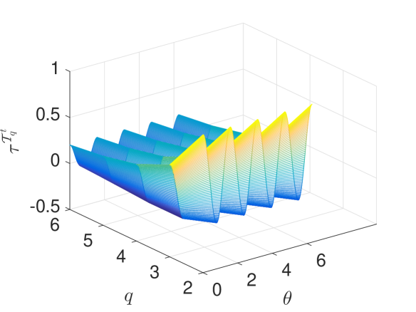
In a similar manner, using the total entropy of Tsallis entropy and its complementary dual, we can define a class of one-parameter entanglement measure, 𝒯qtsubscriptsuperscript𝒯𝑡𝑞\mathcal{T}^{t}_{q}-entropy entanglement, as stated in Appendix B, it also includes the monogamy properties of 𝒯qtsubscriptsuperscript𝒯𝑡𝑞\mathcal{T}^{t}_{q}-entropy entanglement for qubit systems or higher-dimensional systems.

V Entanglement polygon inequalities for quantum networks

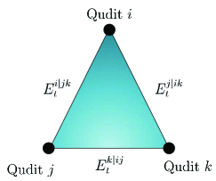
The monogamy inequality (2) provides a lower bound for the corresponding “one-to-group” entanglement, while the polygon inequality provides its upper bound. The polygon inequalities hold for arbitrary qubit pure states with respect to generic entanglement measures Qian2018 . A natural problem is whether the polygon inequalities can be generalized for higher-dimensional systems. A simple geometric interpretation for the inequality (3) is Etj|ik(|ψ),Etk|ij(|ψ)superscriptsubscript𝐸𝑡conditional𝑗𝑖𝑘ket𝜓superscriptsubscript𝐸𝑡conditional𝑘𝑖𝑗ket𝜓E_{t}^{j|ik}(|\psi\rangle),E_{t}^{k|ij}(|\psi\rangle) and Eti|jk(|ψ)superscriptsubscript𝐸𝑡conditional𝑖𝑗𝑘ket𝜓E_{t}^{i|jk}(|\psi\rangle) consist of a triangle, that is, the one-to-group marginal entanglement Etsubscript𝐸𝑡E_{t} can denote the lengths of the three edges of a triangle, as illustrated in Fig.5.
Refer to caption
Figure 5: (Color online) Schematic polygon inequality (3) of tripartite entangled systems. The length of each side denotes correspondingly to the value of the marginal entanglement.

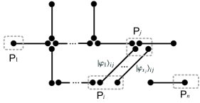
One special scenario to characterize general high-dimensional entangled states is from distributive constructions, where the local tensor structures further can be regarded as quantum networks. In fact, consider an n𝑛n-partite entangled quantum network 𝒩q(𝒫,)subscript𝒩𝑞𝒫\mathcal{N}_{q}(\cal{P},{\cal E}) consisting of bipartite entangled pure states a shown in Fig.6, where 𝒫𝒫\cal{P} represents parties P1,,Pnsubscript𝑃1subscript𝑃𝑛P_{1},\cdots,P_{n}, and {\cal E} denotes entangled states. Suppose that there are sjsubscript𝑠𝑗s_{j} pairs of arbitrary bipartite entangled pure states |φ1ij,|φ2ij,,|φsjijsubscriptketsubscript𝜑1𝑖𝑗subscriptketsubscript𝜑2𝑖𝑗subscriptketsubscript𝜑subscript𝑠𝑗𝑖𝑗|\varphi_{1}\rangle_{ij},|\varphi_{2}\rangle_{ij},\cdots,|\varphi_{s_{j}}\rangle_{ij} shared by any two parties Pisubscript𝑃𝑖P_{i} and Pjsubscript𝑃𝑗P_{j}. Then, the joint state shared by two parties Pisubscript𝑃𝑖P_{i} and Pjsubscript𝑃𝑗P_{j} is given by s=1sj|φsijsubscriptsuperscripttensor-productsubscript𝑠𝑗𝑠1subscriptketsubscript𝜑𝑠𝑖𝑗\mathop{\otimes}^{s_{j}}_{s=1}|\varphi_{s}\rangle_{ij}, the total state of 𝒩q(𝒫,)subscript𝒩𝑞𝒫\mathcal{N}_{q}(\cal{P},{\cal E}) is denoted as

|ΨP1Pn=1i<jnns=1sj|φsij.subscriptketΨsubscript𝑃1subscript𝑃𝑛subscriptsuperscripttensor-product𝑛1𝑖𝑗𝑛subscriptsuperscripttensor-productsubscript𝑠𝑗𝑠1subscriptketsuperscript𝜑𝑠𝑖𝑗\displaystyle|\Psi\rangle_{P_{1}\cdots P_{n}}=\mathop{\otimes}^{n}_{1\leq i<j\leq n}\mathop{\otimes}^{s_{j}}_{s=1}|\varphi^{s}\rangle_{ij}. (73)

Next, we prove the polygon inequality for high-dimensional systems derived from quantum network 𝒩qsubscript𝒩𝑞\mathcal{N}_{q}.

Refer to caption
Figure 6: (Color online). An n𝑛n-partite quantum network consisting of n𝑛n parties P1,,Pnsubscript𝑃1subscript𝑃𝑛P_{1},\cdots,P_{n}. Here, each pair of two parties Pisubscript𝑃𝑖P_{i} and Pjsubscript𝑃𝑗P_{j} share sjsubscript𝑠𝑗s_{j} pairs of bipartite entangled pure states |φ1ij,|φ2ij,,|φsjijsubscriptketsubscript𝜑1𝑖𝑗subscriptketsubscript𝜑2𝑖𝑗subscriptketsubscript𝜑subscript𝑠𝑗𝑖𝑗|\varphi_{1}\rangle_{ij},|\varphi_{2}\rangle_{ij},\cdots,|\varphi_{s_{j}}\rangle_{ij}.
Theorem 2

The polygon inequality of the quantum network 𝒩q(𝒫,)subscript𝒩𝑞𝒫\mathcal{N}_{q}(\cal{P},{\cal E}) is given by

Eti|i¯(|Ψ)jiEtj|j¯(|Ψ),subscriptsuperscript𝐸conditional𝑖¯𝑖𝑡ketΨsubscript𝑗𝑖subscriptsuperscript𝐸conditional𝑗¯𝑗𝑡ketΨ\displaystyle E^{i|\overline{i}}_{t}(|\Psi\rangle)\leq\sum_{j\neq i}E^{j|\overline{j}}_{t}(|\Psi\rangle), (74)

where Eti|i¯subscriptsuperscript𝐸conditional𝑖¯𝑖𝑡E^{i|\overline{i}}_{t} denotes the one-to-group entanglement of the n𝑛n-qudit quantum network state |ΨketΨ|\Psi\rangle, the subscript i𝑖i refers to all the systems owned by the party Pisubscript𝑃𝑖P_{i}, and i¯¯𝑖\overline{i} denotes all the systems except for its owned by Pisubscript𝑃𝑖P_{i}, and Etsubscript𝐸𝑡E_{t} is the Stsuperscript𝑆𝑡S^{t}-entropy entanglement.

Proof. For a given party Pisubscript𝑃𝑖P_{i} in the quantum network 𝒩qsubscript𝒩𝑞\mathcal{N}_{q}, assume that it has entangled with N𝑁N parties Pjsubscript𝑃𝑗P_{j}’s. Instead, suppose there are M𝑀M parties Pksubscript𝑃𝑘P_{k}’s who are entangled with the party Pjsubscript𝑃𝑗P_{j}. It is sufficient to prove that

Eti|i¯(|Ψ)subscriptsuperscript𝐸conditional𝑖¯𝑖𝑡ketΨ\displaystyle E^{i|\overline{i}}_{t}(|\Psi\rangle) =\displaystyle= Et(j=1Ns=1sj|φsij)subscript𝐸𝑡subscriptsuperscripttensor-product𝑁𝑗1subscriptsuperscripttensor-productsubscript𝑠𝑗𝑠1subscriptketsuperscript𝜑𝑠𝑖𝑗\displaystyle E_{t}(\mathop{\otimes}^{N}_{j=1}\mathop{\otimes}^{s_{j}}_{s=1}|\varphi^{s}\rangle_{ij}) (75)
=\displaystyle= S(jρij)\displaystyle S(\otimes_{j}\rho^{j}_{i})
=\displaystyle= S(iρji)\displaystyle S(\otimes_{i}\rho^{i}_{j}) (76)
\displaystyle\leq jiS(kρjk)\displaystyle\sum_{j\neq i}S(\otimes_{k}\rho^{k}_{j}) (77)
=\displaystyle= jiEtj|j¯(|Ψ),subscript𝑗𝑖subscriptsuperscript𝐸conditional𝑗¯𝑗𝑡ketΨ\displaystyle\sum_{j\neq i}E^{j|\overline{j}}_{t}(|\Psi\rangle), (78)

where the state ρij=Tri(|ψijψij|)\rho^{j}_{i}={\rm Tr}_{i}(|\psi\rangle_{ij}\langle\psi\rangle_{ij}|) in Eq.(75) is the reduced density operator for the subsystem of Pisubscript𝑃𝑖P_{i} by tracing out the subsystems of Pjsubscript𝑃𝑗P_{j} entangled with Pisubscript𝑃𝑖P_{i} and |ψij=s=1sj|φsijsubscriptket𝜓𝑖𝑗subscriptsuperscripttensor-productsubscript𝑠𝑗𝑠1subscriptketsubscript𝜑𝑠𝑖𝑗|\psi\rangle_{ij}=\mathop{\otimes}^{s_{j}}_{s=1}|\varphi_{s}\rangle_{ij} is the total state entangled between Pisubscript𝑃𝑖P_{i} and Pjsubscript𝑃𝑗P_{j}. The equality (76) is due to the symmetry in Lemma 1, where the state ρji=Trj(|ψijψij|)\rho^{i}_{j}={\rm Tr}_{j}(|\psi\rangle_{ij}\langle\psi\rangle_{ij}|) is the reduced density operator of the subsystems of Pjsubscript𝑃𝑗P_{j}. The inequality (77) follows from the additivity of separable state ρjksubscriptsuperscript𝜌𝑘𝑗\rho^{k}_{j} in Eq.(19) of Lemma 1, herein, ρjksubscriptsuperscript𝜌𝑘𝑗\rho^{k}_{j} is the reduced density operator for the subsystem of Pjsubscript𝑃𝑗P_{j} by tracing out the subsystems of all the parties Pksubscript𝑃𝑘P_{k}. Here, {Pk}subscript𝑃𝑘\{P_{k}\} denotes all the parties entangled with the given party Pjsubscript𝑃𝑗P_{j}, i.e., the number of {Pi}subscript𝑃𝑖\{P_{i}\} is no more than the numbers of {Pk}subscript𝑃𝑘\{P_{k}\}. \Box

We define the indicator τ𝜏\tau of the Stsuperscript𝑆𝑡S^{t}-entropy marginal entanglement for multipartite quantum system |ΨP1PnsubscriptketΨsubscript𝑃1subscript𝑃𝑛|\Psi\rangle_{P_{1}\cdots P_{n}} as

τEt(|ΨP1Pn)=Eti|i¯(|Ψ)ji,jEtj|j¯(|Ψ).superscript𝜏subscript𝐸𝑡subscriptketΨsubscript𝑃1subscript𝑃𝑛subscriptsuperscript𝐸conditional𝑖¯𝑖𝑡ketΨsubscript𝑗𝑖for-all𝑗subscriptsuperscript𝐸conditional𝑗¯𝑗𝑡ketΨ\displaystyle\tau^{E_{t}}(|\Psi\rangle_{P_{1}\cdots P_{n}})=E^{i|\overline{i}}_{t}(|\Psi\rangle)-\sum_{j\neq i,\forall j}E^{j|\overline{j}}_{t}(|\Psi\rangle). (79)

Example 5. Consider a 333-partite chain quantum network state |ΨABCsubscriptketΨ𝐴𝐵𝐶|\Psi\rangle_{ABC} in Example 3.

The reduced density operator of the subsystem A𝐴A, B𝐵B, and C𝐶C is respectively given by

ϱA=α22|00|+β22|11|+α22|22|+β22|33|,subscriptitalic-ϱ𝐴superscript𝛼22ket0quantum-operator-product0superscript𝛽221quantum-operator-product1superscript𝛼222quantum-operator-product2superscript𝛽223bra3\displaystyle\varrho_{A}=\frac{\alpha^{2}}{2}|0\rangle\langle 0|+\frac{\beta^{2}}{2}|1\rangle\langle 1|+\frac{\alpha^{2}}{2}|2\rangle\langle 2|+\frac{\beta^{2}}{2}|3\rangle\langle 3|,
ϱB=α2|00|+β2|11|,subscriptitalic-ϱ𝐵superscript𝛼2ket0quantum-operator-product0superscript𝛽21bra1\displaystyle\varrho_{B}=\alpha^{2}|0\rangle\langle 0|+\beta^{2}|1\rangle\langle 1|,
ϱC=12|00|+12|11|.subscriptitalic-ϱ𝐶12ket0quantum-operator-product0121bra1\displaystyle\varrho_{C}=\frac{1}{2}|0\rangle\langle 0|+\frac{1}{2}|1\rangle\langle 1|. (80)

From Eq.(22), we get

EtA|BC(|Ψ)=a+b+483log23,subscriptsuperscript𝐸conditional𝐴𝐵𝐶𝑡ketΨ𝑎𝑏483subscript23\displaystyle E^{A|BC}_{t}(|\Psi\rangle)=\frac{a+b+4}{8-3\log_{2}3},
EtB|AC(|Ψ)=α2log2α2β2log2β2,subscriptsuperscript𝐸conditional𝐵𝐴𝐶𝑡ketΨsuperscript𝛼2subscript2superscript𝛼2superscript𝛽2subscript2superscript𝛽2\displaystyle E^{B|AC}_{t}(|\Psi\rangle)=-\alpha^{2}\log_{2}\alpha^{2}-\beta^{2}\log_{2}\beta^{2},
EtC|AB(|Ψ)=1,subscriptsuperscript𝐸conditional𝐶𝐴𝐵𝑡ketΨ1\displaystyle E^{C|AB}_{t}(|\Psi\rangle)=1, (81)

where a𝑎a, b𝑏b are given in Eq.(51). According to Eq.(79) we get

τEt(|Ψ)superscript𝜏subscript𝐸𝑡ketΨ\displaystyle\tau^{E_{t}}(|\Psi\rangle) =\displaystyle= EtA|BC(|Ψ)EtB|AC(|Ψ)EtC|AB(|Ψ).subscriptsuperscript𝐸conditional𝐴𝐵𝐶𝑡ketΨsubscriptsuperscript𝐸conditional𝐵𝐴𝐶𝑡ketΨsubscriptsuperscript𝐸conditional𝐶𝐴𝐵𝑡ketΨ\displaystyle E^{A|BC}_{t}(|\Psi\rangle)-E^{B|AC}_{t}(|\Psi\rangle)-E^{C|AB}_{t}(|\Psi\rangle). (82)

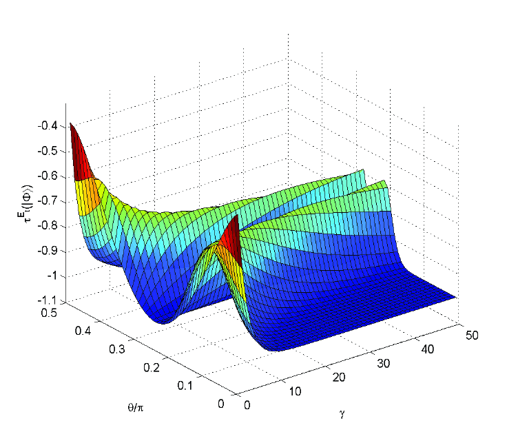
Combining with Eqs.(81) and (82), the indicator τ𝜏\tau of the Stsuperscript𝑆𝑡S^{t}-entropy marginal entanglement is shown in Fig.7. It states that τEt(|Ψ)superscript𝜏subscript𝐸𝑡ketΨ\tau^{E_{t}}(|\Psi\rangle) is negative. This shows Theorem 2 holds for quantum network state defined in Eq.(49).
Refer to caption
Figure 7: (Color online). The indicator τγEtsuperscriptsubscript𝜏𝛾subscript𝐸𝑡\tau_{\gamma}^{E_{t}} of 422tensor-product4224\otimes 2\otimes 2 dimensional system in Example 6. Here, a=cosθ𝑎𝜃a=\cos\theta and b=sinθ𝑏𝜃b=\sin\theta.

VI Conclusion

Entanglement entropy exhibits qualitatively different behaviours from that of classical entropy, and provides a valuable tool for describing the features of many-body states. More importantly, the entanglement entropy measures how a subsystem is entangled with other systems in a given system. In an operational manner, the degree of entanglement in a pure many-body state is quantified by the entanglement entropy of its subsystems. However, until now, most of the entanglement entropies ignore the information of its complement of subsystems. Our consideration in this paper is to propose a new measure from non Neumann entropy and its complement entropy to characterize entanglement. This kind of entanglement shows new features beyond previous entanglement measures. So far, we have considered some special entanglement. A natural problem is to investigate the monogamy relationship for general entanglements, specially for high-dimensional systems.

In conclusion, we proposed the total entropy of the von Neumann entropy and its complementary dual which not only reveals the information of one subsystem but also its complementary statistics. We defined the bipartite Stsuperscript𝑆𝑡S^{t}-entropy entanglement based on the total entropy and provided the analytic formula in two-qubit systems. We also considered the monogamy property of qubit systems and higher-dimensional systems in terms of the Stsuperscript𝑆𝑡S^{t}-entropy entanglement. We obtained a polygon monogamy inequality for arbitrary quantum networks consisting of bipartite entangled pure states. This reveals an intriguing feature of high-dimensional entanglement going beyond any qubit entanglement. These results are interesting in quantum entanglement theory.

Acknowledgments

This work was supported by the National Natural Science Foundation of China (Nos.62172341,61772437), Fundamental Research Funds for the Central Universities (No.2018GF07), and Shenzhen Institute for Quantum Science and Engineering.

References

  • (1) R. Horodecki, P. Horodecki, M. Horodecki, and K. Horodecki, Quantum entanglement, Rev. Mod. Phys. 81, 865 (2009).
  • (2) Y. Zhang, T. Grover, and A. Vishwanath, Entanglement entropy of critical spin liquids, Phys. Rev. Lett. 107, 067202 (2011).
  • (3) S. V. Isakov, M. B. Hastings, and R. G. Melko, Topological entanglement entropy of a Bose-Hubbard spin liquid, Nature Phys. 7, 772-775(2011).
  • (4) D. A. Abanin, and E. Demler, Measuring entanglement entropy of a generic many-body system with a quantum switch, Phys. Rev. lett. 109, 020504 (2012).
  • (5) R. Islam, R. Ma, P. M. Preiss, M. Eric Tai, A. Lukin, M. Rispoli, and M. Greiner, Measuring entanglement entropy in a quantum many-body system, Nature 528, 77-83 (2015).
  • (6) H. Barghathi, C. M. Herdman, and A. Del Maestro, Rényi generalization of the accessible entanglement entropy, Phys. Rev. Lett. 121, 150501 (2018).
  • (7) J. Zhao, Y. C. Wang, Z. Yan, M. Cheng, and Z. Y. Meng, Scaling of entanglement entropy at deconfined quantum criticality, Phys. Rev. Lett. 128, 010601(2022).
  • (8) A. Tavakoli, A. Pozas-Kerstjens, M. X. Luo, M. O. Renou, Bell nonlocality in networks, Rep. Prog. Phys. 85, 056001 (2022).
  • (9) M. A. Nielsen, and I. L. Chuang, Quantum Computation and Quantum Information. Cambridge University Press, Cambridge, 2000.
  • (10) S. Hill, and W. K. Wootters, Entanglement of a pair of quantum bits, Phys. Rev. Lett. 78, 5022-5025 (1997).
  • (11) C. H. Bennett, D. P. DiVincenzo, J. A. Smolin, and W. K. Wootters, Mixed state entanglement and quantum error correction, Phys. Rev. A 54, 3824 (1996).
  • (12) R. Horodecki, P. Horodecki, and M. Horodecki, Quantum α𝛼\alpha-entropy inequalities: independent condition for local realism? Phys. Lett. A 210, 377-381 (1996).
  • (13) G. Gour, S. Bandyopadhyay, and B. C. Sanders, Dual monogamy inequality for entanglement, J. Math. Phys. 48, 012108 (2007).
  • (14) J. S. Kim, and B. C. Sanders, Monogamy of multi-qubit entanglement using Rényi entropy, J. Phys. A: Math. Theor. 43, 445305 (2010).
  • (15) P. T. Landsberg, and V. Vedral, Distributions and channel capacities in generalized statistical mechanics, Phys. Lett. A 247, 211-217 (1998).
  • (16) J. S. Kim, Tsallis entropy and entanglement constraints in multiqubit systems, Phys. Rev. A 81, 062328 (2010).
  • (17) J. S. Kim, and B. C. Sanders, Unified entropy, entanglement measures and monogamy of multi-party entanglement, J. Phys. A Math. Theor. 44, 295303 (2011).
  • (18) V. Coffman, J. Kundu, and W. K. Wootters, Distributed entanglement, Phys. Rev. A 61, 052306 (2000).
  • (19) B. Terhal, Is entanglement monogamous? IBM J. Res. Dev. 48, 71-78 (2004).
  • (20) T. J. Osborne, and F. Verstraete, General monogamy inequality for bipartite qubit entanglement, Phys. Rev. Lett. 96, 220503 (2006).
  • (21) T. R. de Oliveira, M. F. Cornelio, and F. F. Fanchini, Monogamy of entanglement of formation, Phys. Rev. A 89, 034303 (2014).
  • (22) Y. K. Bai, Y. F. Xu, and Z. D. Wang, General monogamy relation for the entanglement of formation in multiqubit systems, Phys. Rev. Lett. 113, 100503 (2014).
  • (23) Y. K. Bai, Y. F. Xu, and Z. D. Wang, Hierarchical monogamy relations for the squared entanglement of formation in multipartite systems, Phys. Rev. A 90, 062343 (2014).
  • (24) W. Song, Y. K. Bai, M. Yang, and Z. L. Cao, General monogamy relation of multi-qubit system in terms of squared Rényi-α𝛼\alpha entanglement, Phys. Rev. A 93, 022306 (2016).
  • (25) Y. Luo, T. Tian, L. H. Shao, and Y. M. Li, General monogamy of Tsallis q𝑞q-entropy entanglement in multiqubit systems, Phys, Rev. A 93, 062340 (2016).
  • (26) A. Khan, J. ur Rehman, K. Wang, and H. Shin, Unified Monogamy Relations of Multipartite Entanglement, Sci. Rep. 9, 16419 (2019).
  • (27) X. N. Zhu, and S. M. Fei, Entanglement monogamy relations of qubit systems, Phys. Rev. A, 90, 024304(2014).
  • (28) Y. Luo, and Y. M. Li, Monogamy of α𝛼\alpha-th power entanglement measurement in qubit system, Ann. Phys. 362, 511-520 (2015).
  • (29) X. Yang, Y. H. Yang, and M. X. Luo, Strong entanglement distribution of quantum networks, Phys. Rev. Research 4, 013153 (2022).
  • (30) X. Yang and M. X. Luo, Unified monogamy relationn of entanglement measures, Quantum Inf. Proc. 20, 108 (2021).
  • (31) M. Christandl, and A. Winter, “Squashed entanglement”: an additive entanglement measure, J. Math. Phys. 45, 829-840(2004).
  • (32) M. Walter, B. Doran, D. Gross, and M. Christandl, Entanglement polytopes: multiparticle entanglement from single-particle information, Science, 340, 1205 (2013).
  • (33) X. F. Qian, M. A. Alonso, and J. H. Eberly, Entanglement polygon inequality in qubit systems, New J. Phys. 20, 063012 (2018).
  • (34) N. Friis, G. Vitagliano, M. Malik, and M. Huber, Entanglement certification from theory to experiment, Nat. Rev. Phys. 1, 72 (2019).
  • (35) N. J. Cerf, M. Bourennane, A. Karlsson, and N. Gisin, Security of quantum key distribution using d𝑑d-level systems, Phys. Rev. Lett. 88, 127902 (2002).
  • (36) L. Sheridan and V. Scarani, Security proof for quantum key distribution using qudit systems, Phys. Rev. A 82, 030301 (2010).
  • (37) M. Mafu, A. Dudley, S. Goyal, D. Giovannini, M. McLaren, M. J. Padgett, T. Konrad, F. Petruccione, N. Lütkenhaus, and A. Forbes, Higher-dimensional orbital-angular-momentum-based quantum key distribution with mutually unbiased bases, Phys. Rev. A 88, 032305 (2013).
  • (38) M. Mirhosseini, O. S. Magaña-Loaiza, M. N. OSullivan, B. Rodenburg, M. Malik, M. P. J. Lavery, M. J. Padgett, D. J. Gauthier, and R. W. Boyd, High-dimensional quantum cryptography with twisted light, New J. Phys. 17, 033033 (2015).
  • (39) N. T. Islam, C. C. W. Lim, C. Cahall, J. Kim, and D. J. Gauthier, Provably secure and high-rate quantum key distribution with time-bin qudits, Sci. Adv. 3, 1701491 (2017).
  • (40) D. Cozzolino, B. Da Lio, D. Bacco, and L. K. Oxenløwe, High-dimensional quantum communication: benefits, progress, and future challenges, Adv. Quant. Tech. 2, 1900038 (2019).
  • (41) M. Erhard, M. Krenn, and A. Zeilinger, Advances in high-dimensional quantum entanglement, Nat. Rev. Phys. 2, 365 (2020).
  • (42) C. E. Shannon, A mathematical theory of communication, Bell System Technical Journal 27, 379-423 (1948).
  • (43) F. Lad, G. Sanfilippo, and G. Agro, Extropy: Complementary dual of entropy, Statistical Sci. 30, 40-58 (2015).
  • (44) N. Canosa and R. Rossignoli, Generalized nonadditive entropies and quantum entanglement, Phys. Rev. Lett. 88, 170401 (2002).
  • (45) C. Tsallis, Possible generalization of Boltzmann-Gibbs statistics, J. Stat. Phys. 52, 479-487 (1988).
  • (46) M. Horodecki, Entanglement measures, Quantum Inf. Comput. 1, 3-26(2001).
  • (47) O. Gühne, and G. Tóth, Entanglement detection, Phys. Rep. 474, 1-75 (2009).
  • (48) G. Vidal, Entanglement monotones, J. Mod. Optics 47, 355-376 (2000).
  • (49) P. Rungta, V. Buzˇˇ𝑧\check{z}ek, C. M. Caves, M. Hillery, and G. J. Milburn, Universal state inversion and concurrence in arbitrary dimensions, Phys. Rev. A 64, 042315 (2001).
  • (50) V. Coffman, J. Kundu, and W. K. Wootters, Distributed entanglement. Phys. Rev. A 61, 052306 (2000).
  • (51) W. K. Wootters, Entanglement of formation of an arbitrary state of two qubits, Phys. Rev. Lett. 80, 2245(1998).
  • (52) L. P. Hughston, R. Jozsa, and W. K. Wootters, A complete classification of quantum ensembles having a given density matrix, Phys. Lett. A 183, 14-18 (1993).
  • (53) A. E. Rastegin, Fano type quantum inequalities in terms of q𝑞q-entropies, Quantum Inf. Proc. 11, 1895-1910 (2012).
  • (54) G. M. Bosyk, S. Zozor, F. Holik, M. Portesi, and P. W. Lamberti, A family of generalized quantum entropies: definition and properties, Quantum Inf. Proc. 15, 3393-3420 (2016).

Appendix A Proof of Lemma 1

The proof is completed by one-by-one.

(i) The quantum total entropy Stsuperscript𝑆𝑡S^{t} for any density matrix ρ𝜌\rho on d𝑑d-dimensional Hilbert space \mathcal{H} satisfies the following inequalities as

0St(ρ)dlog2d(d1)log2(d1).0superscript𝑆𝑡𝜌𝑑subscript2𝑑𝑑1subscript2𝑑1\displaystyle 0\leq S^{t}(\rho)\leq d\log_{2}d-(d-1)\log_{2}(d-1). (83)

Here, the lower bound is achieved only for pure states while the upper bound is reached for the maximally mixed state ρ=𝕀d𝜌𝕀𝑑\rho=\frac{\mathbb{I}}{d}.

Define a function g:[0,1]:𝑔maps-to01g:[0,1]\mapsto\mathbb{R} as

g(x)=xlog2x(1x)log2(1x).𝑔𝑥𝑥subscript2𝑥1𝑥subscript21𝑥\displaystyle g(x)=-x\log_{2}x-(1-x)\log_{2}(1-x). (84)

It is easy to calculate the second derivative of g(x)𝑔𝑥g(x) as

d2g(x)dx2=1x(1x)ln2<0.superscript𝑑2𝑔𝑥𝑑superscript𝑥21𝑥1𝑥20\displaystyle\frac{d^{2}g(x)}{dx^{2}}=-\frac{1}{x(1-x)\ln 2}<0. (85)

This implies that g(x)𝑔𝑥g(x) is a concave function.

From Eq.(10) it follows that

St(ρ)superscript𝑆𝑡𝜌\displaystyle S^{t}(\rho) =\displaystyle= Tr[g(ρ)]Trdelimited-[]𝑔𝜌\displaystyle{\rm Tr}[g(\rho)] (86)
=\displaystyle= ig(λi)subscript𝑖𝑔subscript𝜆𝑖\displaystyle\sum_{i}g(\lambda_{i})
=\displaystyle= di1dg(λi)𝑑subscript𝑖1𝑑𝑔subscript𝜆𝑖\displaystyle d\sum_{i}\frac{1}{d}g(\lambda_{i})
\displaystyle\leq dg(i1dλi)𝑑𝑔subscript𝑖1𝑑subscript𝜆𝑖\displaystyle dg(\sum_{i}\frac{1}{d}\lambda_{i})
=\displaystyle= dg(1d)𝑑𝑔1𝑑\displaystyle dg(\frac{1}{d}) (87)
=\displaystyle= dlog2d(d1)log2(d1).𝑑subscript2𝑑𝑑1subscript2𝑑1\displaystyle d\log_{2}d-(d-1)\log_{2}(d-1). (88)

Here, the inequality (86) is obtained from the concavity of the function g(x)𝑔𝑥g(x) defined in Eq.(84). The equality (87) is followed from the equality of iλi=1subscript𝑖subscript𝜆𝑖1\sum_{i}\lambda_{i}=1. The equality (88) is derived from the definition of g(x)𝑔𝑥g(x) in Eq.(84). This has proved the non-negativity of the total quantum entropy.

(ii) For any convex combination ρ=inpiρi𝜌subscriptsuperscript𝑛𝑖subscript𝑝𝑖subscript𝜌𝑖\rho=\sum^{n}_{i}p_{i}\rho_{i} on finite dimensional Hilbert space ABtensor-productsubscript𝐴subscript𝐵\mathcal{H}_{A}\otimes\mathcal{H}_{B}, we have

inpiSt(ρi)St(ρ),subscriptsuperscript𝑛𝑖subscript𝑝𝑖superscript𝑆𝑡subscript𝜌𝑖superscript𝑆𝑡𝜌\displaystyle\sum^{n}_{i}p_{i}S^{t}(\rho_{i})\leq S^{t}(\rho), (89)

where {pi}subscript𝑝𝑖\{p_{i}\} is a probability distribution, and ρisubscript𝜌𝑖\rho_{i}’s are density matrices on finite dimensional Hilbert space ABtensor-productsubscript𝐴subscript𝐵\mathcal{H}_{A}\otimes\mathcal{H}_{B}. The equality holds if and only if all ρisubscript𝜌𝑖\rho_{i}’s are equal to each other. In fact, for any concave function g(x)𝑔𝑥g(x), the functional p=Tr(g(ρ))𝑝Trg𝜌p=\rm{Tr}(g(\rho)) is concave for any arbitrary Hermitian operator ρ𝜌\rho (see Sec.III in Ref. Rastegin2012 for details). According to Eq.(84), g(x)𝑔𝑥g(x) is concave, that is, the concavity of g𝑔g ensures the concavity of St(ρ)superscript𝑆𝑡𝜌S^{t}(\rho). This has proved the concavity.

(iii) Suppose a pure state |ψABsubscriptket𝜓𝐴𝐵|\psi\rangle_{AB} defined on Hilbert space ABtensor-productsubscript𝐴subscript𝐵{\cal H}_{A}\otimes{\cal H}_{B} has the Schmidt decomposition

|ψ=i=1mλi|aiA|biB.ket𝜓subscriptsuperscript𝑚𝑖1subscript𝜆𝑖subscriptketsubscript𝑎𝑖𝐴subscriptketsubscript𝑏𝑖𝐵\displaystyle|\psi\rangle=\sum^{m}_{i=1}\sqrt{\lambda_{i}}|a_{i}\rangle_{A}|b_{i}\rangle_{B}. (90)

We get that the reduced density matrices ϱAsubscriptitalic-ϱ𝐴\varrho_{A} and ϱBsubscriptitalic-ϱ𝐵\varrho_{B} have the same spectra as {λi}subscript𝜆𝑖\{\lambda_{i}\}. From Eq.(10) it follows that St(ϱA)=St(ϱB)superscript𝑆𝑡subscriptitalic-ϱ𝐴superscript𝑆𝑡subscriptitalic-ϱ𝐵S^{t}(\varrho_{A})=S^{t}(\varrho_{B}) which has proved the symmetry.

(iv) Suppose a mixed state ρ𝜌\rho defined on Hilbert space Asubscript𝐴{\cal H}_{A} has a diagonal form:

ρ=i=1mλi|eiei|,𝜌subscriptsuperscript𝑚𝑖1subscript𝜆𝑖ketsubscript𝑒𝑖brasubscript𝑒𝑖\displaystyle\rho=\sum^{m}_{i=1}\sqrt{\lambda_{i}}|e_{i}\rangle\langle e_{i}|, (91)

where |eiketsubscript𝑒𝑖|e_{i}\rangle are orthogonal states. For a given unitary transformation U𝕊𝕌()𝑈𝕊𝕌U\in\mathbb{SU}({\cal H}), we have UρU=i=1mλi|fifi|𝑈𝜌superscript𝑈subscriptsuperscript𝑚𝑖1subscript𝜆𝑖ketsubscript𝑓𝑖brasubscript𝑓𝑖U\rho U^{\dagger}=\sum^{m}_{i=1}\sqrt{\lambda_{i}}|f_{i}\rangle\langle f_{i}|, where |fi:=U|eiassignketsubscript𝑓𝑖𝑈ketsubscript𝑒𝑖|f_{i}\rangle:=U|e_{i}\rangle are orthogonal states. Note that both ρ𝜌\rho and UρU𝑈𝜌superscript𝑈U\rho U^{\dagger} have the same eigenvalues. Thus from the definition of Stsuperscript𝑆𝑡S^{t}-entropy in Eq.(10) we have concluded the invariance under the unitary operation.

(v) From Ref.Canosa2002 any general entropy function (14) is subadditive if xd2g(x)dx2𝑥superscript𝑑2𝑔𝑥𝑑superscript𝑥2x\frac{d^{2}g(x)}{dx^{2}} is a strictly decreasing function of x(0,1)𝑥01x\in(0,1). From this condition, we can prove the subadditivity of the total quantum entropy Stsuperscript𝑆𝑡S^{t}. In fact, it is easy to check that

dxg′′(x)dx=1(1x)2ln2<0,𝑑𝑥superscript𝑔′′𝑥𝑑𝑥1superscript1𝑥220\displaystyle\frac{dxg^{\prime\prime}(x)}{dx}=-\frac{1}{(1-x)^{2}\ln 2}<0, (92)

where g′′(x)=d2g(x)dx2superscript𝑔′′𝑥superscript𝑑2𝑔𝑥𝑑superscript𝑥2g^{\prime\prime}(x)=\frac{d^{2}g(x)}{dx^{2}} with g(x)𝑔𝑥g(x) defined in Eq.(84). This implies that the quantum entropy Stsuperscript𝑆𝑡S^{t} is subadditive satisfying Eq.(19). Moreover, we can obtain Eq.(20) from Proposition 14 in Ref. Bosyk2016 .

(vi) Consider a given mixed state ρ=ipi|ψiψi|𝜌subscript𝑖subscript𝑝𝑖ketsubscript𝜓𝑖brasubscript𝜓𝑖\rho=\sum_{i}p_{i}|\psi_{i}\rangle\langle\psi_{i}|, where {pi}subscript𝑝𝑖\{p_{i}\} is a probability distribution with ipi=1subscript𝑖subscript𝑝𝑖1\sum_{i}p_{i}=1 and {|ψi}ketsubscript𝜓𝑖\{|\psi_{i}\rangle\} are pure states (orthogonal or nonorthogonal). Then our goal here is to prove

St(ρ)Ht(X),superscript𝑆𝑡𝜌superscript𝐻𝑡𝑋\displaystyle S^{t}(\rho)\leq H^{t}(X), (93)

where Ht(X)superscript𝐻𝑡𝑋H^{t}(X) is the classical total entropy defined as

Ht(X)=i=1n(pilog2pi+(1pi)log2(1pi)),superscript𝐻𝑡𝑋subscriptsuperscript𝑛𝑖1subscript𝑝𝑖subscript2subscript𝑝𝑖1subscript𝑝𝑖subscript21subscript𝑝𝑖\displaystyle H^{t}(X)=-\sum^{n}_{i=1}(p_{i}\log_{2}p_{i}+(1-p_{i})\log_{2}(1-p_{i})), (94)

and X𝑋X is the random variable associated with distribution {p1,p2,,pn}subscript𝑝1subscript𝑝2subscript𝑝𝑛\{p_{1},p_{2},\cdots,p_{n}\}. In fact, denote λjsubscript𝜆𝑗\lambda_{j} and |φjketsubscript𝜑𝑗|\varphi_{j}\rangle as the eigenvalues and the corresponding eigenstate of ρ=jλj|φjφj|𝜌subscript𝑗subscript𝜆𝑗ketsubscript𝜑𝑗brasubscript𝜑𝑗\rho=\sum_{j}\lambda_{j}|\varphi_{j}\rangle\langle\varphi_{j}|. The ensemble classification theorem Hughston1993 states that

|ψi=juijλj|φjketsubscript𝜓𝑖subscript𝑗subscript𝑢𝑖𝑗subscript𝜆𝑗ketsubscript𝜑𝑗\displaystyle|\psi_{i}\rangle=\sum_{j}u_{ij}\sqrt{\lambda_{j}}|\varphi_{j}\rangle (95)

up to a normalization constant, where (uij)subscript𝑢𝑖𝑗(u_{ij}) is a proper unitary matrix. It follows from Eq.(95) and φj|φk=δjkinner-productsubscript𝜑𝑗subscript𝜑𝑘subscript𝛿𝑗𝑘\langle\varphi_{j}|\varphi_{k}\rangle=\delta_{jk}, pi=jwijλjsubscript𝑝𝑖subscript𝑗subscript𝑤𝑖𝑗subscript𝜆𝑗p_{i}=\sum_{j}w_{ij}\lambda_{j}, where wij=uijuijsubscript𝑤𝑖𝑗subscriptsuperscript𝑢𝑖𝑗subscript𝑢𝑖𝑗w_{ij}=u^{\ast}_{ij}u_{ij} are elements of a matrix, i.e., jwij=iwij=1subscript𝑗subscript𝑤𝑖𝑗subscript𝑖subscript𝑤𝑖𝑗1\sum_{j}w_{ij}=\sum_{i}w_{ij}=1 for any i,j𝑖𝑗i,j. Define the function f(x)=g(x)𝑓𝑥𝑔𝑥f(x)=-g(x), that is, f:xg(x):𝑓maps-to𝑥𝑔𝑥f:x\mapsto-g(x)\in\mathbb{R}. f(x)𝑓𝑥f(x) is convex function from the concavity of g(x)𝑔𝑥g(x). Hence, we obtain

if(pi)subscript𝑖𝑓subscript𝑝𝑖\displaystyle\sum_{i}f(p_{i}) =\displaystyle= if(jwijλj)subscript𝑖𝑓subscript𝑗subscript𝑤𝑖𝑗subscript𝜆𝑗\displaystyle\sum_{i}f(\sum_{j}w_{ij}\lambda_{j}) (96)
\displaystyle\leq ijwijf(λj)subscript𝑖subscript𝑗subscript𝑤𝑖𝑗𝑓subscript𝜆𝑗\displaystyle\sum_{i}\sum_{j}w_{ij}f(\lambda_{j})
=\displaystyle= jf(λj),subscript𝑗𝑓subscript𝜆𝑗\displaystyle\sum_{j}f(\lambda_{j}), (97)

where the inequality (96) is followed from the convexity of f(x)𝑓𝑥f(x), the equality is due to iwij=1subscript𝑖subscript𝑤𝑖𝑗1\sum_{i}w_{ij}=1 for all j𝑗j. Combined Eqs.(7) with (10), the inequality (97) implies the inequality (94).

Appendix B The measure based the total entropy of Tsallis entropy and its complementary dual

For the probability distribution p={p1,p2,,pn}psubscript𝑝1subscript𝑝2subscript𝑝𝑛\textbf{p}=\{p_{1},p_{2},\cdots,p_{n}\} of random variable X𝑋X, the Tsallis entropy Tsallis1988 is defined as

Tq(p)=i=1npilnqpisubscript𝑇𝑞psubscriptsuperscript𝑛𝑖1subscript𝑝𝑖subscript𝑞subscript𝑝𝑖\displaystyle T_{q}({\textbf{p}})=-\sum^{n}_{i=1}p_{i}\ln_{q}p_{i} (98)

with one parameter q𝑞q as an extension of shannon entropy. This relation gives the arithmetic mean of the information lnqpisubscript𝑞subscript𝑝𝑖-\ln_{q}p_{i}, with its corresponding probability pisubscript𝑝𝑖p_{i}, where q𝑞q logarithm function is defined by

lnq(x)=1x1qq1subscript𝑞𝑥1superscript𝑥1𝑞𝑞1\displaystyle\ln_{q}(x)=\frac{1-x^{1-q}}{q-1} (99)

for any negative real numbers x𝑥x and q𝑞q. The complementary dual of the Tsallis entropy is defined as

T¯q(p)=i=1n(1pi)lnq(1pi).subscript¯𝑇𝑞psubscriptsuperscript𝑛𝑖11subscript𝑝𝑖subscript𝑞1subscript𝑝𝑖\displaystyle\overline{T}_{q}({\textbf{p}})=-\sum^{n}_{i=1}(1-p_{i})\ln_{q}(1-p_{i}). (100)

Similar with Eq.(7), we define the total entropy of Tsallis entropy and its complementary dual as

Tqt(p)=i=1nTq(pi,1pi),subscriptsuperscript𝑇𝑡𝑞psubscriptsuperscript𝑛𝑖1subscript𝑇𝑞subscript𝑝𝑖1subscript𝑝𝑖\displaystyle T^{t}_{q}({\textbf{p}})=\sum^{n}_{i=1}T_{q}(p_{i},1-p_{i}), (101)

where Tq(pi,1pi)subscript𝑇𝑞subscript𝑝𝑖1subscript𝑝𝑖T_{q}(p_{i},1-p_{i}) are the sum of the Tsallis entropy and its complementary dual of a discrete random variable X𝑋X with a probability distribution {p1,p2,,pn}subscript𝑝1subscript𝑝2subscript𝑝𝑛\{p_{1},p_{2},\cdots,p_{n}\}. Tqtsubscriptsuperscript𝑇𝑡𝑞T^{t}_{q} is also viewed as entropy of the binomial random variable Xi{pi,1pi}similar-tosubscript𝑋𝑖subscript𝑝𝑖1subscript𝑝𝑖X_{i}\sim\{p_{i},1-p_{i}\} with a probability distribution {pi,1pi}subscript𝑝𝑖1subscript𝑝𝑖\{p_{i},1-p_{i}\}.

The quantum entropy of a density operator equals the classical entropy of the probability vector formed by its eigenvalues, thus we give the following definition.

Definition 2

The total entropy of the Tsallis entropy and its complementary dual of a quantum state ρ𝜌\rho on d𝑑d-dimensional Hilbert space {\cal H} is defined by

Tqt(ρ)subscriptsuperscript𝑇𝑡𝑞𝜌\displaystyle T^{t}_{q}(\rho) =\displaystyle= 1TrρqTr(𝟙ρ)q+Tr(𝟙ρ)q1,1Trsuperscript𝜌𝑞Trsuperscript1𝜌𝑞Tr1𝜌𝑞1\displaystyle\frac{1-{\rm Tr}\rho^{q}-{\rm Tr}({\mathbbm{1}-\rho})^{q}+{\rm Tr}({\mathbbm{1}-\rho)}}{q-1}, (102)

which corresponds to with the form (14) with

f(p)=(ppq)+1p(1p)q(q1).𝑓𝑝𝑝superscript𝑝𝑞1𝑝superscript1𝑝𝑞𝑞1\displaystyle f(p)=\frac{(p-p^{q})+1-p-(1-p)^{q}}{(q-1)}. (103)

Here, the function f(p)𝑓𝑝f(p) is a smooth and strictly concave real function on p[0,1]𝑝01p\in[0,1] satisfying f(0)=f(1)=0𝑓0𝑓10f(0)=f(1)=0. For the second derivative of f(p)𝑓𝑝f(p), we have

f′′(p)=q[(1x)q2+pq2]<0superscript𝑓′′𝑝𝑞delimited-[]superscript1𝑥𝑞2superscript𝑝𝑞20\displaystyle f^{\prime\prime}(p)=-q[(1-x)^{q-2}+p^{q-2}]<0 (104)

for any q>0𝑞0q>0. From Ref. Canosa2002 , this entropy satisfies most basic properties of the conventional entropy except for the additivity in Lemma 1.

For a pure state |ΦABsubscriptketΦ𝐴𝐵|\Phi\rangle_{AB} on Hilbert space ABtensor-productsubscript𝐴subscript𝐵{\cal H}_{A}\otimes{\cal H}_{B}, we define its Tqtsubscriptsuperscript𝑇𝑡𝑞T^{t}_{q}-entropy entanglement as

𝒯qt(|ΦAB)=Tqt(ϱA),subscriptsuperscript𝒯𝑡𝑞subscriptketΦ𝐴𝐵subscriptsuperscript𝑇𝑡𝑞subscriptitalic-ϱ𝐴\displaystyle\mathcal{T}^{t}_{q}(|\Phi\rangle_{AB})=T^{t}_{q}(\varrho_{A}), (105)

where ϱA=TrB(|ΦABΦ|)subscriptitalic-ϱ𝐴subscriptTr𝐵subscriptketΦ𝐴𝐵braΦ\varrho_{A}={\rm Tr}_{B}(|\Phi\rangle_{AB}\langle\Phi|) is given in Eq.().

For a bipartite mixed state ρABsubscript𝜌𝐴𝐵\rho_{AB} on Hilbert space ABtensor-productsubscript𝐴subscript𝐵{\cal H}_{A}\otimes{\cal H}_{B}, the Tqtsubscriptsuperscript𝑇𝑡𝑞T^{t}_{q}-entropy entanglement is defined via convex-roof extension

𝒯qt(ρAB)=inf{pi,|Φi}ipi𝒯qt(|ΦiAB),subscriptsuperscript𝒯𝑡𝑞subscript𝜌𝐴𝐵subscriptinfimumsubscript𝑝𝑖ketsubscriptΦ𝑖subscript𝑖subscript𝑝𝑖subscriptsuperscript𝒯𝑡𝑞subscriptketsubscriptΦ𝑖𝐴𝐵\displaystyle\mathcal{T}^{t}_{q}(\rho_{AB})=\inf_{\{p_{i},|\Phi_{i}\rangle\}}\sum_{i}p_{i}\mathcal{T}^{t}_{q}(|\Phi_{i}\rangle_{AB}), (106)

where the infimum is taken over all the possible pure-state decompositions of ρAB=ipi|ΦiABΦi|subscript𝜌𝐴𝐵subscript𝑖subscript𝑝𝑖subscriptketsubscriptΦ𝑖𝐴𝐵brasubscriptΦ𝑖\rho_{AB}=\sum_{i}p_{i}|\Phi_{i}\rangle_{AB}\langle\Phi_{i}|.

In fact, Since Tqtsubscriptsuperscript𝑇𝑡𝑞T^{t}_{q}-entropy complies the general entropic forms, it follows from Proposition 2 in Ref.Canosa2002 that 𝒯qt(ρ)0subscriptsuperscript𝒯𝑡𝑞𝜌0\mathcal{T}^{t}_{q}(\rho)\geq 0 for any density matrix ρ𝜌\rho, where the equality holds if and only if ρ𝜌\rho is separable. On the other hand, the Tqtsubscriptsuperscript𝑇𝑡𝑞T^{t}_{q}-entropy is invariant under local unitary transformation from Proposition 6 in Ref. Canosa2002 . This implies the condition (E2). The concavity of the entropy Tqt(ρ)subscriptsuperscript𝑇𝑡𝑞𝜌T^{t}_{q}(\rho) can be followed from the concavity of the function f(p)𝑓𝑝f(p) in Eq.(103). As a result, the concavity of the Tqtsubscriptsuperscript𝑇𝑡𝑞T^{t}_{q}-entropy ensures the monotonicity of Tqtsubscriptsuperscript𝑇𝑡𝑞T^{t}_{q} under average LOCC, that is, the condition (E3) holds. The convexity (E4) is followed directly from the fact that all the measures constructed via the convex roof extension are convex 3H2009 .

Consider an arbitrary pure state ϕABsubscriptitalic-ϕ𝐴𝐵\phi_{AB} given in Eq.(29), it can be verified that

𝒯qt(|ϕAB)=fq(C(|ϕAB)),subscriptsuperscript𝒯𝑡𝑞subscriptketitalic-ϕ𝐴𝐵subscript𝑓𝑞𝐶subscriptketitalic-ϕ𝐴𝐵\displaystyle\mathcal{T}^{t}_{q}(|\phi\rangle_{AB})=f_{q}(C(|\phi\rangle_{AB})), (107)

where the function fq(x)subscript𝑓𝑞𝑥f_{q}(x) is analytic and defined as

fq(x)subscript𝑓𝑞𝑥\displaystyle f_{q}(x) =\displaystyle= 2[1(1+1x22)q(11x22)q]q1.2delimited-[]1superscript11superscript𝑥22𝑞superscript11superscript𝑥22𝑞𝑞1\displaystyle\frac{2[1-(\frac{1+\sqrt{1-x^{2}}}{2})^{q}-(\frac{1-\sqrt{1-x^{2}}}{2})^{q}]}{q-1}. (108)

This means the 𝒯qtsubscriptsuperscript𝒯𝑡𝑞\mathcal{T}^{t}_{q}-entropy entanglement for qubit systems can be reduced to the Tsallis entropy entanglement. From Ref.Kim2010T , we get a functional relation as

𝒯qt(ρAB)=fq(C(ρAB))subscriptsuperscript𝒯𝑡𝑞subscript𝜌𝐴𝐵subscript𝑓𝑞𝐶subscript𝜌𝐴𝐵\displaystyle\mathcal{T}^{t}_{q}(\rho_{AB})=f_{q}(C(\rho_{AB})) (109)

for a bipartite two-qubit mixed state ρABsubscript𝜌𝐴𝐵\rho_{AB} on Hilbert space ABtensor-productsubscript𝐴subscript𝐵\mathcal{H}_{A}\otimes\mathcal{H}_{B}. Thus, a general monogamy of the Tsallis entropy entanglement in multiqubit systems is naturally inherited by the 𝒯qtsubscriptsuperscript𝒯𝑡𝑞\mathcal{T}^{t}_{q}-entropy entanglement Kim2010T ; Luo2016 . However, the monogamy of multipartite higher-dimensional systems may fail for the 𝒯qtsubscriptsuperscript𝒯𝑡𝑞\mathcal{T}^{t}_{q}-entropy.

Example 6. Consider a 422tensor-product4224\otimes 2\otimes 2 dimensional system in the pure state |ΨABCsubscriptketΨ𝐴𝐵𝐶|\Psi\rangle_{ABC} given in Example 3.

From Eq.(105), we get that

𝒯qt(|ΨA|BC)=2q+1cd2q1(q1),subscriptsuperscript𝒯𝑡𝑞subscriptketΨconditional𝐴𝐵𝐶superscript2𝑞1𝑐𝑑superscript2𝑞1𝑞1\displaystyle\mathcal{T}^{t}_{q}(|\Psi\rangle_{A|BC})=\frac{2^{q+1}-c-d}{2^{q-1}(q-1)}, (110)

where c=α2q2+β2q2𝑐superscript𝛼2𝑞2superscript𝛽2𝑞2c=\alpha^{2q-2}+\beta^{2q-2}, and d=(2α2)q1+(2β2)q1𝑑superscript2superscript𝛼2𝑞1superscript2superscript𝛽2𝑞1d=(2-\alpha^{2})^{q-1}+(2-\beta^{2})^{q-1}. According to Eq.(106), we have

𝒯qt(ρAB)subscriptsuperscript𝒯𝑡𝑞subscript𝜌𝐴𝐵\displaystyle\mathcal{T}^{t}_{q}(\rho_{AB}) =\displaystyle= 2(1α2qβ2q),21superscript𝛼2𝑞superscript𝛽2𝑞\displaystyle 2(1-\alpha^{2q}-\beta^{2q}),
𝒯qt(ρAC)subscriptsuperscript𝒯𝑡𝑞subscript𝜌𝐴𝐶\displaystyle\mathcal{T}^{t}_{q}(\rho_{AC}) =\displaystyle= 2(112q1).211superscript2𝑞1\displaystyle 2(1-\frac{1}{2^{q-1}}). (111)

Thus, the“residual tangle” of the 𝒯qtsubscriptsuperscript𝒯𝑡𝑞\mathcal{T}^{t}_{q}-entropy can be calculated as

τ𝒯qt=𝒯qt(|ΨA|BC)𝒯qt(ρAB)𝒯qt(ρAC).superscript𝜏subscriptsuperscript𝒯𝑡𝑞subscriptsuperscript𝒯𝑡𝑞subscriptketΨconditional𝐴𝐵𝐶subscriptsuperscript𝒯𝑡𝑞subscript𝜌𝐴𝐵subscriptsuperscript𝒯𝑡𝑞subscript𝜌𝐴𝐶\displaystyle\tau^{\mathcal{T}^{t}_{q}}=\mathcal{T}^{t}_{q}(|\Psi\rangle_{A|BC})-\mathcal{T}^{t}_{q}(\rho_{AB})-\mathcal{T}^{t}_{q}(\rho_{AC}). (112)

As its illustrated in Fig.8, different from the τEtsuperscript𝜏superscript𝐸𝑡\tau^{E^{t}} of the Stsuperscript𝑆𝑡S^{t}-entropy entanglement in Fig. 4, the τ𝒯qtsuperscript𝜏subscriptsuperscript𝒯𝑡𝑞\tau^{\mathcal{T}^{t}_{q}} entanglement may be negative or positive, where α=cosθ𝛼𝜃\alpha=\cos\theta and β=sinθ𝛽𝜃\beta=\sin\theta. This means that the generic monogamy does not hold for high-dimensional systems in terms of the 𝒯qtsubscriptsuperscript𝒯𝑡𝑞\mathcal{T}^{t}_{q}-entropy entanglement.

Refer to caption
Figure 8: (Color online). The indicator τ𝒯qtsuperscript𝜏subscriptsuperscript𝒯𝑡𝑞\tau^{\mathcal{T}^{t}_{q}} vias the parameter θ𝜃\theta for a 422tensor-product4224\otimes 2\otimes 2 dimensional system in Example 6.