On the Role of Pre-trained Language Models in Word Ordering:
A Case Study with BART

Abstract

Word ordering is a constrained language generation task taking unordered words as input. Existing work uses linear models and neural networks for the task, yet pre-trained language models have not been studied in word ordering, let alone why they help. We use BART as an instance and show its effectiveness in the task. To explain why BART helps word ordering, we extend analysis with probing and empirically identify that syntactic dependency knowledge in BART is a reliable explanation. We also report performance gains with BART in the related partial tree linearization task, which readily extends our analysis.

1 Introduction

The task of word ordering Wan et al. (2009); Zhang and Clark (2015); Tao et al. (2021), also known as linearization Liu et al. (2015), aims to assign a valid permutation to a bag of words for a coherent sentence. While early work uses word ordering to improve the grammaticality of machine-generated sentences Wan et al. (2009), the task subsequently manifests itself in applications such as discourse generation Althaus et al. (2004), machine translation Tromble and Eisner (2009); He and Liang (2011), and image captioning Fang et al. (2015). It plays a central role in linguistic realization Gatt and Krahmer (2018) of pipeline text generation systems. Advances in word ordering are also relevant to retrieval augmented generation Guu et al. (2020), with outputs additionally conditioned on retrieved entries, which can constitute a bag of words.

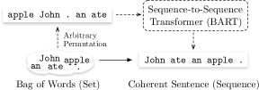
Figure 1: Illustration of our approach for word ordering. Bag-of-words inputs are first turned into pseudo-sequences with arbitrarily word permutations, and then fed to a sequence-to-sequence Transformer for coherent outputs.

Word ordering can be viewed as constrained language generation with all inflected output words provided, which makes it more amenable for error analysis (section 3.4). The task can be extended to tree linearization He et al. (2009) or partial tree linearization Zhang (2013) with syntactic features as additional input. Syntactic models Liu et al. (2015) and language models Schmaltz et al. (2016) have been used in word ordering to rank candidate word permutations. Recently, Hasler et al. (2017) and Tao et al. (2021) explore different designs of neural models for the task. However, no existing studies investigate pre-trained language models (PLMs; Qiu et al. 2020) for word ordering, which have effectively improved various NLP tasks.

Intuitively, the rich knowledge in PLMs can readily help word ordering. However, the unordered bag-of-words inputs may seem incompatible to PLMs with sequential inputs. The role of PLMs in word ordering thus remains an interesting research question. We fill the research gap by empirically investigating BART Lewis et al. (2020), a pre-trained sequence-to-sequence Transformer Vaswani et al. (2017), as an instance of PLMs for word ordering. Specifically, we assign an arbitrary permutation for the input bag of words to obtain a pseudo-sequence, and use sequence-to-sequence Transformers to generate ordered outputs, as illustrated in Figure 1. As BART uses subword inputs Sennrich et al. (2016) instead of words Schmaltz et al. (2016); Hasler et al. (2017); Tao et al. (2021), we implement constrained beam search using prefix trees (section 3.1; Figure 2). Results show that BART substantially improves word ordering compared to our Transformer baseline, which already outperforms previous best (section 3.3).

With Transformer models (including BART), we further investigate consequences of two major modeling decisions, which remain unexamined in the literature. First, while all previous studies assume output sequences constrained within permutations of input words, Tao et al. (2021) eliminate such constraints. We find the latter leads to a consistent performance drop, which is further attributed to missing words in outputs, a phenomenon related to the coverage issue in machine translation Tu et al. (2016). Second, Hasler et al. (2017) use conditional probability $p(\boldsymbol{y}|\boldsymbol{x})$ instead of the unconditional one $p(\boldsymbol{y})$ of Schmaltz et al. (2016) to score candidate output permutations $\boldsymbol{y}$ of input bag of words $\boldsymbol{x}$. We provide the first fair comparison for the two approaches, and find that with small decoding beam, conditional models substantially outperform unconditional ones. Interestingly, such an advantage fails to persist as we increase the beam size.

Our Transformer word orderers may be sensitive to arbitrary word permutations in the input pseudo-sequence (section 3.6). Recent studies Sinha et al. (2021); Ettinger (2020) show that Transformers are relatively insensitive to word permutations in sequential inputs. They are more sensitive to local orders than global orders of input subwords on the GLUE benchmark Clouâtre et al. (2021). In contrast, we find that Transformer (including BART) word orderers are relatively insensitive to both word and subword permutations in inputs. Such result can be relevant to modeling unordered inputs with PLMs Castro Ferreira et al. (2020); Lin et al. (2020).

We finally aim to explain why BART helps word ordering (section 4). Analysis with probing Rogers et al. (2020) provides speculated explanations for the utility of PLMs with the possession of numerous types of knowledge. However, for a reliable explanation, we need to identify the specific type of knowledge relevant to the task. In addition, the amount of the knowledge should be nontrivial in the PLM. With a procedure based on feature importance Fraser et al. (2014) and probing Hewitt and Manning (2019), we empirically identify that knowledge about syntactic dependency structure reliably explains why BART helps word ordering. Our analysis can be readily extended to partial tree linearization Zhang (2013), for which we also report performance gains with our models (section 5).

2 Related Work

Word Ordering Modeling

Early work uses syntactic models Zhang and Clark (2011); Liu et al. (2015) and language models Zhang et al. (2012); Liu and Zhang (2015) to rank candidate permutations of input words. Liu and Zhang (2015) and Schmaltz et al. (2016) discuss their relative importance. Syntactic models rank candidates with the probability of the jointly predicted parse tree. They can be linear models Wan et al. (2009) or neural networks Song et al. (2018) with hand-crafted features. Language models use the probability of the output sentence for ranking. Early work uses statistical n-gram models Zhang et al. (2012), which are later replaced by recurrent neural networks Schmaltz et al. (2016). Most related to our work, Hasler et al. (2017) and Tao et al. (2021) formulate word ordering as conditional generation. Hasler et al. (2017) uses an LSTM decoder with attention Bahdanau et al. (2015) and an encoder degenerating to an embedding layer. Tao et al. (2021) stack self-attention Vaswani et al. (2017) layers as the encoder and use a decoder from pointer network See et al. (2017). Both encode bag-of-words inputs with permutation invariant word encoders. In contrast, we turn bag-of-words inputs into subword pseudo-sequences and feed them to standard sequence-to-sequence models. Instead of investigating features, prediction targets, and model architectures as in previous work, we focus on the utility of BART in the task.

Word Ordering Decoding

Early work relies on time-constrained best-first-search White (2005); Zhang and Clark (2011). As it lacks an asymptotic upper bound for time complexity Liu et al. (2015), later work with syntactic models Song et al. (2018), language models Schmaltz et al. (2016), and conditional generation models Hasler et al. (2017); Tao et al. (2021) adopt beam search for decoding. All previous work assumes an output space constrained to permutations of input words except for Tao et al. (2021), who assume the output to be any sequences permitted by the vocabulary. However, the effect of such unconstrained output space is unexamined. We compare the difference between beam search with constrained and unconstrained output spaces.

Tasks Related to Word Ordering

Word ordering was first proposed by Bangalore et al. (2000) as a surrogate for grammaticality test, and later formulated by Wan et al. (2009) as a standard task. A closely related task is CommonGen Lin et al. (2020), which aims to generate a coherent sentence subjective to commonsense constraints given a set of lemmatized concept words. In contrast, word ordering is a constrained language modeling task given inflected output words. Tree linearization He et al. (2009) is a related task with full dependency trees as inputs. Dropping subsets of dependency arcs and part-of-speech tags results in partial tree linearization Zhang (2013). Further removing functional words and word inflections results in surface realization Mille et al. (2020). Different from CommonGen and surface realization, the provided output bag-of-words limit reliance on domain knowledge and reduce ambiguity in output, making word ordering a concentrated case for testing generic linguistic capacity Raji et al. (2021) of text generation models. In addition, word ordering requires no labeling in contrast to all these tasks.

PLMs and Non-Sequential Inputs

PLMs with the Transformer Vaswani et al. (2017) decoder are amenable for sequence generation Raffel et al. (2020); Lewis et al. (2020). They have been used for sequence generation tasks with non-sequential inputs, such as AMR-to-Text Mager et al. (2020), RDF-to-Text Ribeiro et al. (2021), and CommonGen Lin et al. (2020). Typically, non-sequential inputs are turned into sequential ones before being fed to PLMs. Additionally aiming to understand why BART helps word ordering, we adopt a similar approach and refrain from task-specific engineering, which allows the same sequence-to-sequence model for multiset and tree inputs, limiting extra confounding factors in our analysis.

Analysis with Probing

Previous work on probing Rogers et al. (2020) has identified various types of knowledge in PLMs, such as syntax Hewitt and Manning (2019), semantics Tenney et al. (2019), and commonsense Roberts et al. (2020). They are speculated to explain the utility of PLMs in target tasks. We make such explanations reliable for BART in word ordering by establishing the relevance of specific types of knowledge to the task, in addition to probing their existence in BART.

3 Word Ordering with BART

We describe our formulation of word ordering and how to adopt the sequence-to-sequence BART for the task (section 3.1), report results on the standard PTB benchmark (sections 3.2 and 3.3), and analyze effects of different modeling decisions (sections 3.5, 3.4 and 3.6).

3.1 Modeling Word Ordering

We formulate word ordering as conditional generation following Hasler et al. (2017). The input bag of words constitutes a multiset $\boldsymbol{x}$, where different elements can take the same value. The probability of output sequence $\boldsymbol{y}$, conditioning on $\boldsymbol{x}$, is parameterized by $\theta$ and factorizes auto-regressively:

$$p_{\theta}(\boldsymbol{y}|\boldsymbol{x})=\prod_{t}p_{\theta}(y_{t}|\boldsymbol{y}_{<t},\boldsymbol{x})$$ (1)

where $\boldsymbol{y}_{<t}$ consists of previous generated tokens up to step $t-1$, the next token $y_{t}$ takes a token from the output vocabulary. Output sequences start with a special token $y_{0}$ denoting beginning of sentences. Following Hasler et al. (2017), after solving $\theta$ with maximum likelihood estimation on the training set, we use beam search in an output space for the candidate $\boldsymbol{y}$ maximizing the product $\prod_{t}p_{\theta}(y_{t}|\boldsymbol{y}_{<t},\boldsymbol{x})$.

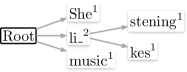
Figure 2: Prefix tree at initialization for constraints {“She”, “li_ kes”, “li_ stening”, “music”}. Each path from the root to a leaf corresponds to a subword sequence. Except for the root, each node corresponds to a subword and tracks its count (superscript) in the constraints. A pointer (bold outline) denoting the previously generated subword $y_{t-1}$ points to the root at initialization. At decoding step $t$, only subwords of child nodes with nonzero count are valid as the next token $y_{t}$. Once a subword is selected for $y_{t}$, we move the pointer to the corresponding node and decrement its count by 1. The pointer is reset to the root after reaching leaves. Decoding for each candidate finishes when all counts are zero.

Output sequences $\boldsymbol{y}$’s are generally constrained within permutations of input words Schmaltz et al. (2016); Tao et al. (2021). To account for corrupted inputs (e.g., word deletion), Tao et al. (2021) use an unconstrained output space with any sequence permitted by the vocabulary. We analyze the output difference between decoding with constrained and unconstrained output space in section 3.4.

Beam search with bag-of-words constraints can be simply implemented by tracking words to be generated using a multiset for each candidate in the beam and setting $p_{\theta}(y_{t}|\boldsymbol{y}_{<t},\boldsymbol{x})$ of invalid (not in the multiset) next words to zero. The generated word $y_{t}$ are then removed from the multiset after decoding step $t$. Decoding of each candidate ends with an empty multiset. Different from previous work Schmaltz et al. (2016); Hasler et al. (2017); Tao et al. (2021), subword segmentation of BART turns each input word into a sequence of subwords, which poses sequential constraints on the output. Thus tracking generated subwords and eliminate invalid next subwords during beam search require a different data structure. We compile subword sequences into a prefix tree as illustrated in Figure 2, where counts at nodes track subwords to be generated and child nodes correspond to valid next subwords. See Figure 6 in Appendix A for a concrete working example.

Conditional models use $p_{\theta}(y_{t}|\boldsymbol{y}_{<t},\boldsymbol{x})$ to score the next token $y_{t}$ given previously generated tokens $\boldsymbol{y}_{<t}$. They additionally depend on the input $\boldsymbol{x}$, which helps track words to be generated and mitigate the ambiguity of selecting $y_{t}$. In contrast, unconditional models Schmaltz et al. (2016) with probability $p_{\theta}(y_{t}|\boldsymbol{y}_{<t})$ only depend on local information $y_{t}$ and $\boldsymbol{y}_{<t}$, which can lead to high ambiguity of selecting $y_{t}$ and attract beam search with small beams to local minimums. In section 3.5, we analyze the difference between conditional and unconditional models with a fair comparison.

To instantiate $p_{\theta}(\boldsymbol{y}|\boldsymbol{x})$, we use a Transformer Vaswani et al. (2017) consisting of both encoder and decoder pre-trained with BART Lewis et al. (2020). Transformers use self-attention, a permutation invariant layer, to model contextual representations for input tokens. Vaswani et al. (2017) add distinct position embeddings onto input token embeddings at different positions to make self-attention sensitive to input orders. BART pre-trains Transformers to reconstruct corrupted input sequences. As BART assumes sequential inputs, we convert the multiset input $\boldsymbol{x}$ into a pseudo-sequence by assigning an arbitrary permutation to the input words, following Lin et al. (2020); see Figure 1 for an illustration. Although subword orders within each word are informative, Transformers (and BART) may be sensitive to the arbitrary word permutation in the input. We analyze the permutation sensitivity of our models in section 3.6.

3.2 Settings and Implementations

Following previous work Hasler et al. (2017); Tao et al. (2021), we use PTB sections 2-21 (39,832 sentences) for training, section 22 (1,700 sentences) for development, and section 23 (2,416 sentences) for test. Punctuation escapes of PTB are reverted to match the vocabulary of BART. We randomly shuffle words of each output sentence to create the input and perform BPE segmentation Sennrich et al. (2016) for both input and output. BLEU Papineni et al. (2002) are reported as the performance metric following Schmaltz et al. (2016). Our implementation is based on fairseq Ott et al. (2019).

We train a Transformer from scratch (denoted RAND) as the baseline and compared it to the finetuned BART base (denoted BART) to estimate gains from BART pre-training. Hyperparameters are tuned separately since different models have different optimums. We find vocabulary size 8000 optimal for RAND. Both models share identical architecture with 6-layer encoder and decoder. RAND (35 million parameters) has smaller hidden size 512 and feed-forward hidden size 1024 compared to 756 and 3072 of BART (140 million parameters). They both need heavy regularization: $\beta=0.3$ for label smoothing Pereyra et al. (2017), $p=0.3$ for dropout Srivastava et al. (2014), and $\alpha=1$ for R-drop Liang et al. (2021). Both models are trained using Adam Kingma and Ba (2015). We use 100 samples per batch, 4000 warm-up steps and learning rate 5e-4 for RAND; 20 samples per batch, 1000 warm-up steps and learning rate 1e-4 for BART. Learning rate decays with the inverse square root of training steps. We train the model till the development loss stops improving and average the last 5 checkpoints saved per 1000 training steps. We use beam size 64 to search on a constrained output space without additional specification. For unconstrained output space, we use beam size 64 and length normalization Murray and Chiang (2018).

Settings	B=5	B=64	B=512
Unconstrained
AttnM	34.89	/	/
RAND-ours	38.53	38.95	39.04
BART-ours	54.29	54.86	54.84
Constrained
Ngram	23.3	/	35.7
RNNLM	24.5	34.6	38.6
Bag	33.4	36.2	37.1
RAND-ours	38.97	39.52	39.59
BART-ours	54.70	56.38	56.63

Table 1: Test BLEU for word ordering on PTB. B=X denotes standard beam search with beam size X. Attn, Bag and our models are all conditional models while Ngram and RNNLM are unconditional ones.

3.3 Word Ordering Results

We compare our results with previous work under similar settings: for conditional models, bag2seq (Bag; Hasler et al. 2017) and AttM (AttnM; Tao et al. 2021) are included; for unconditional models, we include N-gram language models (Ngram) and RNNLM (RNNLM; Schmaltz et al. 2016) reproduced by Hasler et al. (2017). Except for AttnM, all models use a constrained output space. We do not consider heuristically tailored beam search Schmaltz et al. (2016); Hasler et al. (2017) and focus on standard sequence-to-sequence modeling. Different from existing studies, we use BPE segmentation for all our settings.

As shown in Table 1, our baseline RAND outperforms previous best results with unconstrained (38.53 of RAND compared to 34.89 of AttnM with B=5) and constrained (39.59 of RAND compared to 38.6 of RNNLM with B=512) output space, showing the effectiveness of sequence-to-sequence modeling with Transformer. Compared to RAND, BART brings substantial improvements under different settings, with up to 17.04 BLEU using B=512 and constrained output space, which demonstrates the effectiveness of BART pre-training for word ordering, setting the stage for later analyses.

Figure 3: Test lexical errors of RAND with beam size 5 using unconstrained output space. We show the proportions of missing/redundant words and the output length ratios for test instances binned with output lengths. For the complete test set, the rates of missing and redundant words are 5.74% and 3.3%, respectively. The output length ratio is 0.981. See Figure 7 in section B.1 for the results of different settings and how the metrics are computed.

3.4 Errors of Unconstrained Output Space

We can readily examine the output lexical errors by comparing the input and output bag of words. As shown in Figure 3, beam search with unconstrained output space tends to miss input words rather than generate redundant words. The tendency becomes prominent when increasing the output length, accompanied by a slight drop in the output length ratio. These lexical errors explain the consistent performance drop compared to constrained output space in Table 1. See section B.1 for additional results. The related coverage issue for sequence-to-sequence models has been studied in machine translation Tu et al. (2016); Mi et al. (2016). However, different from word ordering, an error-prone source-target alignment procedure is required to estimate the output bag of words.

3.5 Effects of Conditional Modeling

We argued in section 3.1 that conditional modeling is less ambiguous when selecting the next token $y_{t}$, avoiding local minimum during beam search and thus performing well with small beams. Such a hypothesis is suggested by previous results included in Table 1: the conditional model Bag substantially outperforms (+8.9) the unconditional RNNLM with B=5; unconditional models require large beams to perform well Schmaltz et al. (2016). We verify these observations with a fair comparison. Concretely, we feed a null token as the input to simulate unconditional modeling with sequence-to-sequence models and train the models with the same settings in section 3.2.

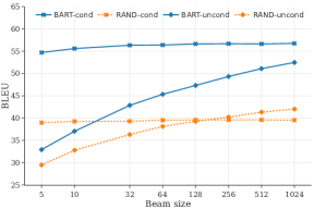
Figure 4: Test BLEU of conditional (cond) and unconditional (uncond) modeling with RAND and BART, using different beam size. A null token is fed to the encoder to simulate unconditional modeling.

Results are shown in Figure 4. With small beams, conditional models substantially outperform unconditional models. Unconditional models heavily rely on large beams to perform well. In contrast, small beams perform on par with large beams for conditional models. These results verify our hypothesis. Interestingly, as the beam size further increases, RAND-uncond slightly outperforms RAND-cond, showing that a larger candidate space can address ambiguities from local modeling $p_{\theta}(y_{t}|\boldsymbol{y}_{<t})$ to some extent, at the expense of extra computation and memory overhead.

[font=] Bob & eats & food
NNP & VBZ & NNP
[edge unit distance=2.6ex]2root [edge unit distance=3ex]12sub [edge unit distance=3ex]32obj

(a) Dependency tree

base	food Bob eat_ s
brac	( food ) ( Bob ) ( eat_ s )
pos	( food NNP ) ( Bob NNP ) ( eat_ s VBZ )
udep	( eat_ s ( Bob ) ( food ) )
ldep	( eat_ s :sub ( Bob ) :obj ( food ) )
full	( eat_ s VBZ :obj ( food NNP ) :sub ( Bob NNP ) )

(b) BPE tokenized PENMMAN notation sequences

Figure 5: An example dependency tree and its BPE tokenized PENMAN notation sequences with different features.

3.6 Effects of Input Permutations

We empirically investigate the permutation sensitivity of our models for word ordering. The sensitivity is estimated with BLEU from 10 different development sets, each with distinct input word permutations. We compare our models to several controlled settings. The first is data augmentation: for each training instance, we created augmented samples with the same target output but different input word permutations, denoted aug. The second is a Transformer without encoder position embeddings, which is invariant to input subword permutations, denoted npos. To examine the importance of subword sequences, we also train RAND and BART with input subwords shuffled, denoted shuf. All models are trained with the same settings in section 3.2.

Results are shown in Table 2. Both RAND and BART with the baseline setting base are relatively insensitive to different input word permutations (with standard deviation 0.133 and 0.185), compared to the controlled setting npos (with standard deviation 0.05). Data augmentations aug2-aug8 marginally improves the mean BLEU compared to base, but no consistent decrease of the standard deviation is observed. See section B.2 for similar results with unconstrained output space. Surprisingly, with constrained output space, the lost local subword orders in npos and shuf has little impact on the performance, in contrast to the findings of Clouâtre et al. (2021). Even marginal improvement for BART is observed (56.45 with shuf compared to 56.21 with base). However, with unconstrained output space, the loss of local subword orders results in a non-trivial drop in performance. See section B.2 for detailed results.

Settings	RAND	BART
base	40.45 (0.133)	56.21 (0.185)
aug2	40.86 (0.159)	56.78 (0.110)
aug4	40.73 (0.088)	56.97 (0.164)
aug6	40.73 (0.157)	56.76 (0.180)
aug8	40.94 (0.104)	56.91 (0.155)
npos	40.05 (0.050)	/
shuf	39.58 (0.135)	56.45 (0.133)

Table 2: Permutation sensitivity measured by the mean and standard deviation (in the bracket) of BLEU on 10 development sets with distinct input word permutations. Results are obtained with constrained output space; for unconstrained output space see Table 6 in section B.2. base denotes settings in section 3.2. augx is trained with additional x augmented samples per training instance. npos removes encoder position embeddings. shuf is trained with shuffled input subwords.

4 Understanding Why BART Helps

We empirically establish the intuition that knowledge in BART helps target tasks. Though numerous types of knowledge have been identified in PLMs by probing Rogers et al. (2020), they may not necessarily improve the target task Cífka and Bojar (2018). Thus a reliable explanation should identify the relevant type of knowledge for word ordering. Candidate types of knowledge can be selected using a procedure akin to feature importance (section 4.1): we feed different types of knowledge as additional features and select the one bringing the most salient gain in word ordering. Their relevance should be further verified by a strong correlation (section 4.2) between the probing performance and word ordering performance, as models can utilize unexpected shortcut rules Geirhos et al. (2020) instead of distilling the intended knowledge provided in the features. Such a correlation is estimated using models with different amount of the knowledge. We finally probe for the nontrivial existence of the knowledge in BART (section 4.2).

4.1 Analysis with Feature Importance

We first select a candidate type of knowledge for our explanation. Based on empirical evidence Liu et al. (2015) and linguistic theories de Marneffe and Nivre (2019), we narrow our focus to syntactic dependencies. Nevertheless, different parts of a dependency tree can be the candidate: brackets around words (brac), part-of-speech tags (pos), dependency structure (udep), labeled dependency structure (ldep), and the full tree with labeled dependency structure and part-of-speech tags (full). Knowledge are injected into models by feeding it as additional input feature. The resulting performance gain compared to the baseline (base) with bag-of-words inputs indicates the importance of the feature Fraser et al. (2014), a surrogate for the relevance of the type of knowledge.

Dependency trees are derived from the PTB following Zhang (2013), with tags defined by Nivre et al. (2007). We use the same data split as in section 3.2. Bag-of-words inputs with additional features are turned into PENMAN notation sequences Mager et al. (2020) and fed to sequence-to-sequence Transformers as in section 3.1; see Figure 5 for input examples. For tree-structured inputs, we shuffle the children of each head nodes before turning them into sequences. Dependency labels and part-of-speech tags are kept intact during BPE tokenization. We follow the same settings in section 3.2 to train RAND and BART with additional input features.

Results are shown in Table 3. The additional features from different types of knowledge consistently improves word ordering, among which dependency structure (udep) brings the main performance gain (comparing udep to base, RAND is improved by 47.15 and BART by 34.37), suggesting the potential relevance of the knowledge to word ordering. Further adding dependency labels and part-of-speech tags marginally helps (comparing ldep and full to udep, RAND and BART are improved by up to 2.79 and 1.20, respectively). Interestingly, although part-of-speech tags alone slightly help (comparing pos to base, RAND is improved by 2.04 and BART by 1.49), their benefits diminish given dependency structures (comparing ldep to full, RAND is improved by 0.03 while BART dropping 0.27), suggesting that dependency structure knowledge can subsume part-of-speech tags. Accordingly, we select knowledge about dependency structure as our candidate for explanation.

4.2 Analysis with Structural Probing

To obtain a reliable explanation, we then establish the correlation between dependency structure knowledge in the model and word ordering performance, and verify the existence of the knowledge in BART. Both require examining dependency structure knowledge in models, which can be achieved by the structural probe Hewitt and Manning (2019), a learned bilinear distance metric taking representations of a model as input features. It estimates the unlabeled dependency trees of sentences using minimum spanning trees. The resulting unlabeled attachment score (UAS) indicates the probing performance. We use the average UAS of representations from all decoder layers to indicate the dependency structure knowledge in the model. We omit encoder representations since matching unordered input words to ground truth dependencies is ambiguous. Decoder representations are obtained by feeding the ground-truth outputs to the model. For each output token $y_{t}$, one can choose representations that predict it ($\mathbf{h}(\boldsymbol{y}_{<t},\boldsymbol{x})$) or from feeding it ($\mathbf{h}(\boldsymbol{y}_{<t+1},\boldsymbol{x})$) as features. We use the former as it results in higher UAS in our preliminary experiments. Features of words are the average of their subword features.

We follow the default hyperparameters of Hewitt and Manning (2019), with a rank of 32, and train with the L1 loss for 30 epochs using 40 samples per batch. We use the derived dependency trees from section 4.1 as our dataset and report the averaged UAS on the PTB test set. Since dependency structure knowledge can subsume part-of-speech tags as shown in section 4.1, feeding features of base, pos or udep to RAND and BART results in models with varied amounts of the knowledge. Their structural probing results are shown in Table 4.

Settings	RAND	BART	$\Delta_{\texttt{B}-\texttt{R}}$
base	40.36	56.14	15.78
brac	40.58 +  0.22	56.64 +  0.50	16.06
pos	42.40 +  2.04	57.63 +  1.49	15.23
udep	87.51 +47.15	90.51 +34.37	3.00
ldep	90.27 +49.91	91.70 +35.56	1.43
full	90.30 +49.94	91.43 +35.29	1.13

Table 3: Development BLEU with different input syntactic features: brac for brackets around words, pos for part-of-speech tags, udep and ldep for unlabeled and labeled dependencies, and full for part-of-speech tags and labeled dependencies. Performance gains against bag-of-words inputs (base) are shown in the superscripts. The $\Delta_{\texttt{B}-\texttt{R}}$ column is the differences between BART and RAND.

The consistent probing performance gains on feeding additional features in Table 4 confirms that knowledge is indeed injected into the models by feature feeding, ruling out the possibility that models use shortcut rules (with pos, RAND is improved by 1.26 and BART by 0.87; with udep, RAND is improved by 10.17 and BART by 12.13). Jointly examining Table 3 and Table 4, we find that an increase in UAS always corresponds to improved BLEU. The Pearson’s correlation coefficient of 0.8845 between BLEU and UAS further verifies that dependency structure knowledge is relevant to word ordering across settings.

We finally compare the probing performance of BART initialized with pre-trained parameters (with UAS 53.06) to the agnostic setting using randomly initialized token embeddings (with 42.59 UAS). The performance gap of 10.47 indicates that a nontrivial amount of dependency structure knowledge exists in BART. The relevance to word ordering and the existence in BART make knowledge about syntactic dependency structure a reliable explanation for the utility of BART in word ordering.

5 Extension to Partial Tree Linearization

Our analysis in section 4 can be readily extended to partial tree linearization Zhang (2013), a generalized word ordering task provided with additional syntactic input features. Unlike settings in section 4, additional features can be arbitrary subsets of part-of-speech tags and labeled dependency arcs. The task can be helpful for applications such as machine translation Zhang et al. (2014). Following Zhang (2013), we use the same dependency trees in section 4.1 and report BLEU on the PTB development set with different proportions of syntactic features.

Previous studies Zhang (2013); Puduppully et al. (2016) use linear models with hand-crafted features. Each base noun phrase (BNP; noun phrases without decedent noun phrases) is regarded as a single word for computation efficiency. We adopt the same sequence-to-sequence models RAND and BART in section 3.2 and report results with and without special treatment for BNPs. Similar to section 4.1, partial trees are turned into PENMAN sequences and fed to sequence-to-sequence Transformers. We use the same model for different proportions of input features. For each tree in the training set, we sample 0%, 50% and 100% of part-of-speech tags and labeled dependency arcs, respectively, resulting in 9 training instances with different input features for the same ordered output sequence. To keep inputs consistent, we put brackets around words that have no additional features (see brac in Figure 5).

Settings	RAND	BART	$\Delta_{\texttt{B}-\texttt{R}}$
base	44.69	53.05	8.36
pos	45.95 +  1.26	53.83 +  0.78	7.88
udep	54.86 +10.17	65.18 +12.13	10.32

Table 4: Averaged UAS of all decoder layers (including the embedding) on test set. base, pos and udep are the same as Table 3. Performance gains against base are shown in the superscript. The differences between BART and RAND are shown in the $\Delta_{\texttt{B}-\texttt{R}}$ column.

Results are shown in Table 5. For comparison, we include results of Puduppully et al. (2016), denoted P16, and Zhang (2013), denoted Z13. We notice that treating BNPs as words substantially simplifies the task: the mean BLEU increase from 59.5 to 73.0 for RAND and from 73.7 to 82.5 for BART. RAND substantially outperforms the previous best result of P16 by 6.8 mean BLEU. In addition, BART brings further improvements by 9.5 mean BLEU, giving a new best-reported result.

Settings	(0, 0)	(0.5, 0)	(1, 0)	(0, 0.5)	(0.5, 0.5)	(1, 0.5)	(0, 1)	(0.5, 1)	(1, 1)	Mean
Z13†	42.9	43.4	44.7	50.5	51.4	52.2	73.3	74.7	76.3	56.6
P16†	48.0	49.0	51.5	59.0	62.0	67.1	82.8	86.2	89.9	66.2
RAND†	58.8	59.5	59.7	72.0	72.6	72.6	87.1	87.1	87.3	73.0
BART†	71.7	71.9	72.3	83.2	83.1	83.2	92.1	92.4	92.2	82.5
RAND	42.0	42.4	42.8	55.2	55.6	56.8	80.1	80.1	80.5	59.5
BART	55.9	56.5	57.2	73.6	73.6	73.6	90.9	90.8	90.9	73.7

Table 5: Development BLEU with constrained output space for partial tree linearization with different proportions of (pos, ldep) input features. Settings with † treat a BNP as a single word.

6 Conclusion

We investigated the role of PLMs in word ordering using BART as an instance. Non-sequential inputs are turned into sequences and fed to sequence-to-sequence Transformers and BART for coherent outputs. We achieve the best-reported results on word ordering and partial tree linearization with BART. With Transformers and BART, we provide a systematic study on the effects of output space constraints, conditional modeling, and permutation sensitivity of inputs for word ordering. Our findings can shed light on related pre-trained models such as T5 Raffel et al. (2020) in related tasks such as CommonGen. Our analysis with feature importance and structural probing empirically identifies that knowledge about syntactic dependency structure reliably explains the utility of BART in word ordering. Such a procedure is general and can be readily used to explain why a given PLM helps a target task.

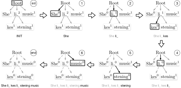
Figure 6: Illustration of how the constraint prefix tree in Figure 2 of a path is updated during decoding. We omit the state of resetting the pointer to root for brevity. At initialization, the count of each node corresponds to how many times the subword appears in the input. At step 1, as “She” is a valid subword selected by beam search, we move the pointer the node of “She” and decrement its count by 1. In the following steps, “She” becomes invalid as its count becomes zero. After step 6, since counts in all children of the root become zeros, the path is marked finished.

Appendix A Beam Search with Output Constraints

The standard beam search is modify by tracking the state of a candidate with a constraint prefix tree, which specifies valid next tokens at each decoding step. The update rules for the prefix tree are described in Figure 2. See Figure 6 for an illustration of how the constraint tree for a candidate in the beam is updated during decoding.

Settings	RAND	BART
base	39.39 (0.151)	59.79 (0.158)
aug2	39.50 (0.118)	60.00 (0.152)
aug4	40.08 (0.091)	60.00 (0.167)
aug6	39.73 (0.053)	59.86 (0.154)
aug8	40.02 (0.152)	59.64 (0.170)
npos	36.98 (0.018)
shuf	36.52 (0.186)	58.34 (0.124)

Table 6: Permutation sensitivity measured by the mean and standard deviation (in the bracket) of BLEU on 10 development sets with distinct input word permutations. Results are obtained with unconstrained output space. Settings are the same as Table 2.

Appendix B Results of Unconstrained Output Space

We include additional results with unconstrained output space to complement the discussion in section 3.4 and section 3.6.

B.1 Lexical Errors

In addition to Figure 3 in section 3.4, we present results for different models and beam sizes in Figure 7. Redundant (missing) words are all words in predicted (reference) output but not in reference (predicted) outputs. We normalize the count with number of words in all reference. Length ratio is ratio of predicted output length to reference output length.

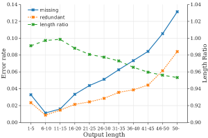
(a) RAND,B=5: missing 5.74%, redundant 3.30%, length ratio 0.981.

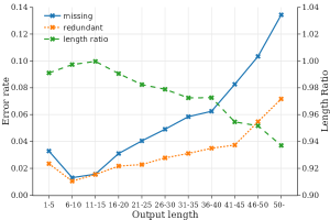
(b) RAND,B=512: missing 5.42%, redundant 3.02%, length ratio 0.982.

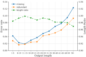
(c) BART,B=5: missing 5.30%, redundant 4.16%, length ratio 0.990.

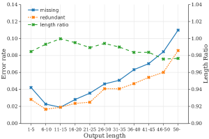
(d) BART,B=512: missing 4.89%, redundant 3.85%, length ratio 0.991.

Figure 7: Test lexical errors with unconstrained output space similar to Figure 3 for additional models and settings. We show the proportions of missing/redundant words and the output length ratios for test instances binned with output lengths. The model, beam size, and results on the complete test set are shown in the caption.

B.2 Permutation Sensitivity

We replicate results of Table 2 in section 3.6 with unconstrained output space in Table 6. Similar to Table 2, data augmentation brings marginal improvement on mean BLEU and no consistent drop in standard deviation. Unlike Table 2, the loss of subword sequences results in a nontrivial drop in performance, especially for RAND (-2.87 from base to shuf). BART is less sensitive to subword shuffling (-1.45 from base to shuf).

References

- Althaus et al. (2004) Ernst Althaus, Nikiforos Karamanis, and Alexander Koller. 2004. Computing locally coherent discourses. In Proceedings of the 42nd Annual Meeting of the Association for Computational Linguistics (ACL-04), pages 399–406, Barcelona, Spain.
- Bahdanau et al. (2015) Dzmitry Bahdanau, Kyunghyun Cho, and Yoshua Bengio. 2015. Neural machine translation by jointly learning to align and translate. In 3rd International Conference on Learning Representations, ICLR 2015, San Diego, CA, USA, May 7-9, 2015, Conference Track Proceedings.
- Bangalore et al. (2000) Srinivas Bangalore, Owen Rambow, and Steve Whittaker. 2000. Evaluation metrics for generation. In INLG’2000 Proceedings of the First International Conference on Natural Language Generation, pages 1–8, Mitzpe Ramon, Israel. Association for Computational Linguistics.
- Castro Ferreira et al. (2020) Thiago Castro Ferreira, Claire Gardent, Nikolai Ilinykh, Chris van der Lee, Simon Mille, Diego Moussallem, and Anastasia Shimorina. 2020. The 2020 bilingual, bi-directional WebNLG+ shared task: Overview and evaluation results (WebNLG+ 2020). In Proceedings of the 3rd International Workshop on Natural Language Generation from the Semantic Web (WebNLG+), pages 55–76, Dublin, Ireland (Virtual). Association for Computational Linguistics.
- Cífka and Bojar (2018) Ondřej Cífka and Ondřej Bojar. 2018. Are BLEU and meaning representation in opposition? In Proceedings of the 56th Annual Meeting of the Association for Computational Linguistics (Volume 1: Long Papers), pages 1362–1371, Melbourne, Australia. Association for Computational Linguistics.
- Clouâtre et al. (2021) Louis Clouâtre, Prasanna Parthasarathi, Amal Zouaq, and Sarath Chandar. 2021. Demystifying neural language models’ insensitivity to word-order. ArXiv preprint, abs/2107.13955.
- de Marneffe and Nivre (2019) Marie-Catherine de Marneffe and Joakim Nivre. 2019. Dependency grammar. Annual Review of Linguistics, 5(1):197–218.
- Ettinger (2020) Allyson Ettinger. 2020. What BERT is not: Lessons from a new suite of psycholinguistic diagnostics for language models. Transactions of the Association for Computational Linguistics, 8:34–48.
- Fang et al. (2015) Hao Fang, Saurabh Gupta, Forrest N. Iandola, Rupesh Kumar Srivastava, Li Deng, Piotr Dollár, Jianfeng Gao, Xiaodong He, Margaret Mitchell, John C. Platt, C. Lawrence Zitnick, and Geoffrey Zweig. 2015. From captions to visual concepts and back. In IEEE Conference on Computer Vision and Pattern Recognition, CVPR 2015, Boston, MA, USA, June 7-12, 2015, pages 1473–1482. IEEE Computer Society.
- Fraser et al. (2014) Kathleen C. Fraser, Graeme Hirst, Naida L. Graham, Jed A. Meltzer, Sandra E. Black, and Elizabeth Rochon. 2014. Comparison of different feature sets for identification of variants in progressive aphasia. In Proceedings of the Workshop on Computational Linguistics and Clinical Psychology: From Linguistic Signal to Clinical Reality, pages 17–26, Baltimore, Maryland, USA. Association for Computational Linguistics.
- Gatt and Krahmer (2018) Albert Gatt and Emiel Krahmer. 2018. Survey of the state of the art in natural language generation: Core tasks, applications and evaluation. J. Artif. Intell. Res., 61:65–170.
- Geirhos et al. (2020) Robert Geirhos, Jörn-Henrik Jacobsen, Claudio Michaelis, Richard Zemel, Wieland Brendel, Matthias Bethge, and Felix A. Wichmann. 2020. Shortcut learning in deep neural networks. Nature Machine Intelligence, 2(11):665–673.
- Guu et al. (2020) Kelvin Guu, Kenton Lee, Zora Tung, Panupong Pasupat, and Ming-Wei Chang. 2020. Realm: Retrieval-augmented language model pre-training. arXiv:2002.08909 [cs]. ArXiv: 2002.08909.
- Hasler et al. (2017) Eva Hasler, Felix Stahlberg, Marcus Tomalin, Adrià de Gispert, and Bill Byrne. 2017. A comparison of neural models for word ordering. In Proceedings of the 10th International Conference on Natural Language Generation, pages 208–212, Santiago de Compostela, Spain. Association for Computational Linguistics.
- He and Liang (2011) Jing He and Hongyu Liang. 2011. Word-reordering for statistical machine translation using trigram language model. In Proceedings of 5th International Joint Conference on Natural Language Processing, pages 1288–1293, Chiang Mai, Thailand. Asian Federation of Natural Language Processing.
- He et al. (2009) Wei He, Haifeng Wang, Yuqing Guo, and Ting Liu. 2009. Dependency based Chinese sentence realization. In Proceedings of the Joint Conference of the 47th Annual Meeting of the ACL and the 4th International Joint Conference on Natural Language Processing of the AFNLP, pages 809–816, Suntec, Singapore. Association for Computational Linguistics.
- Hewitt and Manning (2019) John Hewitt and Christopher D. Manning. 2019. A structural probe for finding syntax in word representations. In Proceedings of the 2019 Conference of the North American Chapter of the Association for Computational Linguistics: Human Language Technologies, Volume 1 (Long and Short Papers), pages 4129–4138, Minneapolis, Minnesota. Association for Computational Linguistics.
- Kingma and Ba (2015) Diederik P. Kingma and Jimmy Ba. 2015. Adam: A method for stochastic optimization. In 3rd International Conference on Learning Representations, ICLR 2015, San Diego, CA, USA, May 7-9, 2015, Conference Track Proceedings.
- Levin (2018) Janet Levin. 2018. Functionalism. In Edward N. Zalta, editor, The Stanford Encyclopedia of Philosophy, Fall 2018 edition. Metaphysics Research Lab, Stanford University.
- Lewis et al. (2020) Mike Lewis, Yinhan Liu, Naman Goyal, Marjan Ghazvininejad, Abdelrahman Mohamed, Omer Levy, Veselin Stoyanov, and Luke Zettlemoyer. 2020. BART: Denoising sequence-to-sequence pre-training for natural language generation, translation, and comprehension. In Proceedings of the 58th Annual Meeting of the Association for Computational Linguistics, pages 7871–7880, Online. Association for Computational Linguistics.
- Liang et al. (2021) Xiaobo Liang, Lijun Wu, Juntao Li, Yue Wang, Qi Meng, Tao Qin, Wei Chen, Min Zhang, and Tie-Yan Liu. 2021. R-drop: Regularized dropout for neural networks. arXiv:2106.14448 [cs]. ArXiv: 2106.14448.
- Lin et al. (2020) Bill Yuchen Lin, Wangchunshu Zhou, Ming Shen, Pei Zhou, Chandra Bhagavatula, Yejin Choi, and Xiang Ren. 2020. CommonGen: A constrained text generation challenge for generative commonsense reasoning. In Findings of the Association for Computational Linguistics: EMNLP 2020, pages 1823–1840, Online. Association for Computational Linguistics.
- Liu and Zhang (2015) Jiangming Liu and Yue Zhang. 2015. An empirical comparison between n-gram and syntactic language models for word ordering. In Proceedings of the 2015 Conference on Empirical Methods in Natural Language Processing, pages 369–378, Lisbon, Portugal. Association for Computational Linguistics.
- Liu et al. (2015) Yijia Liu, Yue Zhang, Wanxiang Che, and Bing Qin. 2015. Transition-based syntactic linearization. In Proceedings of the 2015 Conference of the North American Chapter of the Association for Computational Linguistics: Human Language Technologies, pages 113–122, Denver, Colorado. Association for Computational Linguistics.
- Mager et al. (2020) Manuel Mager, Ramón Fernandez Astudillo, Tahira Naseem, Md Arafat Sultan, Young-Suk Lee, Radu Florian, and Salim Roukos. 2020. GPT-too: A language-model-first approach for AMR-to-text generation. In Proceedings of the 58th Annual Meeting of the Association for Computational Linguistics, pages 1846–1852, Online. Association for Computational Linguistics.
- Mi et al. (2016) Haitao Mi, Baskaran Sankaran, Zhiguo Wang, and Abe Ittycheriah. 2016. Coverage embedding models for neural machine translation. In Proceedings of the 2016 Conference on Empirical Methods in Natural Language Processing, pages 955–960, Austin, Texas. Association for Computational Linguistics.
- Mille et al. (2020) Simon Mille, Anya Belz, Bernd Bohnet, Thiago Castro Ferreira, Yvette Graham, and Leo Wanner. 2020. The third multilingual surface realisation shared task (SR’20): Overview and evaluation results. In Proceedings of the Third Workshop on Multilingual Surface Realisation, pages 1–20, Barcelona, Spain (Online). Association for Computational Linguistics.
- Murray and Chiang (2018) Kenton Murray and David Chiang. 2018. Correcting length bias in neural machine translation. In Proceedings of the Third Conference on Machine Translation: Research Papers, pages 212–223, Brussels, Belgium. Association for Computational Linguistics.
- Nivre et al. (2007) Joakim Nivre, Johan Hall, Jens Nilsson, Atanas Chanev, Gülşen Eryi̇gi̇t, Sandra Kübler, Svetoslav Marinov, and Erwin Marsi. 2007. Maltparser: A language-independent system for data-driven dependency parsing. Natural Language Engineering, 13(2):95–135.
- Ott et al. (2019) Myle Ott, Sergey Edunov, Alexei Baevski, Angela Fan, Sam Gross, Nathan Ng, David Grangier, and Michael Auli. 2019. fairseq: A fast, extensible toolkit for sequence modeling. In Proceedings of the 2019 Conference of the North American Chapter of the Association for Computational Linguistics (Demonstrations), pages 48–53, Minneapolis, Minnesota. Association for Computational Linguistics.
- Papineni et al. (2002) Kishore Papineni, Salim Roukos, Todd Ward, and Wei-Jing Zhu. 2002. Bleu: a method for automatic evaluation of machine translation. In Proceedings of the 40th Annual Meeting of the Association for Computational Linguistics, pages 311–318, Philadelphia, Pennsylvania, USA. Association for Computational Linguistics.
- Pereyra et al. (2017) Gabriel Pereyra, George Tucker, Jan Chorowski, Lukasz Kaiser, and Geoffrey E. Hinton. 2017. Regularizing neural networks by penalizing confident output distributions. In 5th International Conference on Learning Representations, ICLR 2017, Toulon, France, April 24-26, 2017, Workshop Track Proceedings. OpenReview.net.
- Puduppully et al. (2016) Ratish Puduppully, Yue Zhang, and Manish Shrivastava. 2016. Transition-based syntactic linearization with lookahead features. In Proceedings of the 2016 Conference of the North American Chapter of the Association for Computational Linguistics: Human Language Technologies, pages 488–493, San Diego, California. Association for Computational Linguistics.
- Qiu et al. (2020) Xipeng Qiu, Tianxiang Sun, Yige Xu, Yunfan Shao, Ning Dai, and Xuanjing Huang. 2020. Pre-trained models for natural language processing: A survey. ArXiv preprint, abs/2003.08271.
- Raffel et al. (2020) Colin Raffel, Noam Shazeer, Adam Roberts, Katherine Lee, Sharan Narang, Michael Matena, Yanqi Zhou, Wei Li, and Peter J. Liu. 2020. Exploring the limits of transfer learning with a unified text-to-text transformer. J. Mach. Learn. Res., 21:140:1–140:67.
- Raji et al. (2021) Inioluwa Deborah Raji, Emily Denton, Emily M. Bender, Alex Hanna, and Amandalynne Paullada. 2021. AI and the everything in the whole wide world benchmark. In Thirty-fifth Conference on Neural Information Processing Systems Datasets and Benchmarks Track (Round 2).
- Ribeiro et al. (2021) Leonardo F. R. Ribeiro, Martin Schmitt, Hinrich Schütze, and Iryna Gurevych. 2021. Investigating pretrained language models for graph-to-text generation. In Proceedings of the 3rd Workshop on Natural Language Processing for Conversational AI, pages 211–227, Online. Association for Computational Linguistics.
- Roberts et al. (2020) Adam Roberts, Colin Raffel, and Noam Shazeer. 2020. How much knowledge can you pack into the parameters of a language model? In Proceedings of the 2020 Conference on Empirical Methods in Natural Language Processing (EMNLP), pages 5418–5426, Online. Association for Computational Linguistics.
- Rogers et al. (2020) Anna Rogers, Olga Kovaleva, and Anna Rumshisky. 2020. A primer in BERTology: What we know about how BERT works. Transactions of the Association for Computational Linguistics, 8:842–866.
- Schmaltz et al. (2016) Allen Schmaltz, Alexander M. Rush, and Stuart Shieber. 2016. Word ordering without syntax. In Proceedings of the 2016 Conference on Empirical Methods in Natural Language Processing, pages 2319–2324, Austin, Texas. Association for Computational Linguistics.
- See et al. (2017) Abigail See, Peter J. Liu, and Christopher D. Manning. 2017. Get to the point: Summarization with pointer-generator networks. In Proceedings of the 55th Annual Meeting of the Association for Computational Linguistics (Volume 1: Long Papers), pages 1073–1083, Vancouver, Canada. Association for Computational Linguistics.
- Sennrich et al. (2016) Rico Sennrich, Barry Haddow, and Alexandra Birch. 2016. Neural machine translation of rare words with subword units. In Proceedings of the 54th Annual Meeting of the Association for Computational Linguistics (Volume 1: Long Papers), pages 1715–1725, Berlin, Germany. Association for Computational Linguistics.
- Sinha et al. (2021) Koustuv Sinha, Robin Jia, Dieuwke Hupkes, Joelle Pineau, Adina Williams, and Douwe Kiela. 2021. Masked language modeling and the distributional hypothesis: Order word matters pre-training for little. arXiv:2104.06644 [cs]. ArXiv: 2104.06644.
- Song et al. (2018) Linfeng Song, Yue Zhang, and Daniel Gildea. 2018. Neural transition-based syntactic linearization. In Proceedings of the 11th International Conference on Natural Language Generation, pages 431–440, Tilburg University, The Netherlands. Association for Computational Linguistics.
- Srivastava et al. (2014) Nitish Srivastava, Geoffrey E. Hinton, Alex Krizhevsky, Ilya Sutskever, and Ruslan Salakhutdinov. 2014. Dropout: a simple way to prevent neural networks from overfitting. J. Mach. Learn. Res., 15(1):1929–1958.
- Tao et al. (2021) Chongyang Tao, Shen Gao, Juntao Li, Yansong Feng, Dongyan Zhao, and Rui Yan. 2021. Learning to organize a bag of words into sentences with neural networks: An empirical study. In Proceedings of the 2021 Conference of the North American Chapter of the Association for Computational Linguistics: Human Language Technologies, pages 1682–1691, Online. Association for Computational Linguistics.
- Tenney et al. (2019) Ian Tenney, Patrick Xia, Berlin Chen, Alex Wang, Adam Poliak, R. Thomas McCoy, Najoung Kim, Benjamin Van Durme, Samuel R. Bowman, Dipanjan Das, and Ellie Pavlick. 2019. What do you learn from context? probing for sentence structure in contextualized word representations. In 7th International Conference on Learning Representations, ICLR 2019, New Orleans, LA, USA, May 6-9, 2019. OpenReview.net.
- Tromble and Eisner (2009) Roy Tromble and Jason Eisner. 2009. Learning linear ordering problems for better translation. In Proceedings of the 2009 Conference on Empirical Methods in Natural Language Processing, pages 1007–1016, Singapore. Association for Computational Linguistics.
- Tu et al. (2016) Zhaopeng Tu, Zhengdong Lu, Yang Liu, Xiaohua Liu, and Hang Li. 2016. Modeling coverage for neural machine translation. In Proceedings of the 54th Annual Meeting of the Association for Computational Linguistics (Volume 1: Long Papers), pages 76–85, Berlin, Germany. Association for Computational Linguistics.
- Vaswani et al. (2017) Ashish Vaswani, Noam Shazeer, Niki Parmar, Jakob Uszkoreit, Llion Jones, Aidan N. Gomez, Lukasz Kaiser, and Illia Polosukhin. 2017. Attention is all you need. In Advances in Neural Information Processing Systems 30: Annual Conference on Neural Information Processing Systems 2017, December 4-9, 2017, Long Beach, CA, USA, pages 5998–6008.
- Wan et al. (2009) Stephen Wan, Mark Dras, Robert Dale, and Cécile Paris. 2009. Improving grammaticality in statistical sentence generation: Introducing a dependency spanning tree algorithm with an argument satisfaction model. In Proceedings of the 12th Conference of the European Chapter of the ACL (EACL 2009), pages 852–860, Athens, Greece. Association for Computational Linguistics.
- White (2005) Michael White. 2005. Designing an extensible API for integrating language modeling and realization. In Proceedings of Workshop on Software, pages 47–64, Ann Arbor, Michigan. Association for Computational Linguistics.
- Zhang (2013) Yue Zhang. 2013. Partial-tree linearization: Generalized word ordering for text synthesis. In IJCAI 2013, Proceedings of the 23rd International Joint Conference on Artificial Intelligence, Beijing, China, August 3-9, 2013, pages 2232–2238. IJCAI/AAAI.
- Zhang et al. (2012) Yue Zhang, Graeme Blackwood, and Stephen Clark. 2012. Syntax-based word ordering incorporating a large-scale language model. In Proceedings of the 13th Conference of the European Chapter of the Association for Computational Linguistics, pages 736–746, Avignon, France. Association for Computational Linguistics.
- Zhang and Clark (2011) Yue Zhang and Stephen Clark. 2011. Syntax-based grammaticality improvement using CCG and guided search. In Proceedings of the 2011 Conference on Empirical Methods in Natural Language Processing, pages 1147–1157, Edinburgh, Scotland, UK. Association for Computational Linguistics.
- Zhang and Clark (2015) Yue Zhang and Stephen Clark. 2015. Discriminative syntax-based word ordering for text generation. Computational Linguistics, 41(3):503–538.
- Zhang et al. (2014) Yue Zhang, Kai Song, Linfeng Song, Jingbo Zhu, and Qun Liu. 2014. Syntactic SMT using a discriminative text generation model. In Proceedings of the 2014 Conference on Empirical Methods in Natural Language Processing (EMNLP), pages 177–182, Doha, Qatar. Association for Computational Linguistics.