$T_{2}$-limited dc Quantum Magnetometry via Flux Modulation

Abstract

High-sensitivity magnetometry is of critical importance to the fields of biomagnetism and geomagnetism. However, the magnetometry for the low-frequency signal detection meets the challenge of sensitivity improvement, due to multiple types of low-frequency noise sources. In particular, for the solid-state spin quantum magnetometry, the sensitivity of low frequency magnetic field has been limited by short $T_{2}^{*}$. Here, we demonstrate a $T_{2}$-limited dc quantum magnetometry based on the nitrogen-vacancy centers in diamond. The magnetometry, combining the flux modulation and the spin-echo protocol, promotes the sensitivity from being limited by $T_{2}^{*}$ to $T_{2}$ of orders of magnitude longer. The sensitivity of the dc magnetometry of 32 $\rm pT/Hz^{1/2}$ has been achieved, overwhelmingly improved by 100 folds over the Ramsey-type method result of 4.6 $\rm nT/Hz^{1/2}$. Further enhancement of the sensitivity have been systematically analyzed, although challenging but plenty of room is achievable. Our result sheds light on realization of room temperature dc quantum magnetomerty with femtotesla-sensitivity in the future.

Sensing weak magnetic fields plays an important role in many frontier science and technology, such as biological signal measurement Boto2018 ; Cohen1967 , geomagnetic survey Lenz2006 , magnetic imaging applications Glenn2017 , and exotic interactions examination Jiao2021 . Quantum sensors have been proposed with high sensitivity and other advantages Degen2017 ; Budker2007 ; Dolabdjian2017 ; Dolabdjian2017 . In particular, a type of solid-state spin system, the electron spins of Nitrogen-Vacancy (NV) centers in diamond, has been proposed to be utilized as a quantum magnetometry with potential sensitivity up to femtotesla at room temperature Taylor2008 . Since then, great efforts have been paid to enhance its sensitivity for detecting static or low-frequency magnetic fields, including cavity-enhanced infrared absorption magnetometry Jensen2014 ; Chatzidrosos2017 , the total internal reflection Clevenson2015 , flux concentration Xie2021 ; Fescenko2020 , and continuously excited Ramsey measurements combined with lock-in detection Zhang2021c . The NV-based magnetometry has been improved to be sub-picotesla sensitivity Xie2021 ; Fescenko2020 with flux concentration and picotesla sensitivityBarry2017 without flux concentration.

There is still a great gap between the current low-frequency sensitivity and the expected femotesla-sensitivity for NV-based magnetometry. The main obstacle is the short $T_{2}^{*}$ of the ensemble NV center system, which essentially limits sensitivities of the continuous wave type and Ramsey-type NV-based magnetometers. Recently, intense efforts have been paid to increase $T_{2}^{*}$ by improving the material of the diamond or by developing advanced quantum control technologies Barry2020 ; Bauch2018 ; Wolf2015 ; Bauch2018 ; Zhang2021c . Schemes have been proposed to break the $T_{2}^{*}$ limit, including the ancilla-assisted frequency up-conversion Liu2019a and fast rotation of diamonds Wood2018a . By dynamically engineering quantum states of NV centers, these works turn the static magnetic field into a pseudo ac one. However, significant sensitivity advancement still remains elusive.

In this work, a dc quantum magnetometry with $T_{2}$-limited based on the ensemble of NV centers in diamond is demonstrated. A Flux Concentration and Modulation (FCM) technique has been utilized to transfer the dc magnetic signal to an ac one. Then the ac signal can be detected with the spin-echo sequence Hahn1950 applied on the NV magnetometry. Our work has achieved a $\sim$140 folds sensitivity enhancement from 4.6 $\rm nT/Hz^{1/2}$ to 32 $\rm pT/Hz^{1/2}$. The low-frequency sensitivity limit has been successfully boosted from $T_{2}^{*}$ to $T_{2}$. We also systematically analyzed limitations for enhancement of the sensitivity with the current magnetometry, and our result paves a way towards future realization of room temperature dc quantum magnetomerty with femotesla-sensitivity.

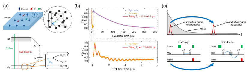
Fig. 1: The system of the NV centers in diamond and the basic idea of our scheme. (a) Diagram of diamond containing NV centers and other impurities. ¹³C and N_s represent for isotope of carbon atom and isolated substitutional nitrogen atom in diamond lattice, respectively. (b) Experimental results of Ramsey experiment and spin-echo experiment. The data of Ramsey experiment is fitted by exponential damping and sum of three cosine function with different angular frequency. $T_{2}^{*}=1.13\pm 0.03~{}\rm\mu s$ is obtained. The oscillation in $T_{2}^{*}$ data is induced by the hyperfine interaction between NV and ¹⁴N. The data of spin-echo signal is fitted by exponential damping function and get $T_{2}=102.0\pm 0.5~{}\rm\mu s$. (c) The schematic of the magnetic field modulation. The raw external signal is in the low-frequency domain originally, while the low-frequency noise and spin bath noise are dominant. The modulation method transfers the raw signal into high-frequency domain. The noise in the high-frequency domain presents less intensity compared to the low-frequency domain.

The NV center consists of a substitutional nitrogen adjacent to a lattice vacancy. The energy levels of NV center is shown in Fig. 1(a). The ground state of NV center is a spin triplet state ${}^{3}A_{2}$, which contains sublevels of $m_{s}=0$ and $m_{s}=\pm 1$ Barry2020 . The excited state of NV center includes some discrete electronic states and continuous vibronic states with higher energy. A 532 nm laser can be used to excite the NV center. Then the NV center decays to the ground state with fluorescence emitting from 600 to 850 nm Barry2020 . The intensity of fluorescence is dependent on the spin state of NV center in ground state. Thus the readout of NV center can be realized by the 532 nm laser excitation and fluorescence acquisition.

There are many types of impurities in the diamond, such as ¹³C and N_s shown in Fig. 1(a). The inevitable interactions between these impurities and the electron spin of NV center are the main contributions to the short dephasing time $T_{2}^{*}$. In our experiment, the $T_{2}^{*}$ is $1.13\pm 0.03~{}\rm\mu s$ (Fig. 1(b)). This dephasing effect can be greatly suppressed by dynamical decoupling technique such as spin-echo sequence, and the coherence time of the NV centers can be prolonged to $T_{2}$. The prolonged coherence time $T_{2}$ with spin-echo sequence is $102.0\pm 0.5~{}\rm\mu s$ (Fig. 1(b)). Unfortunately, the dynamical decoupling technique also cancels the effect of dc magnetic field on NV centers. Therefore, the prolonged coherence time via dynamical decoupling technique cannot ensure the improvement of the dc magnetic sensitivity of the NV magnetometry. In this work, we utilized the FCM method to transfer the low-frequency signal into the high-frequency domain, while the Ramsey-type protocol can be replaced by the spin-echo protocol accordingly, as demonstrated in Fig. 1(c). Our method will result in an extending limit to $T_{2}$ for the low-frequency magnetic field detection.

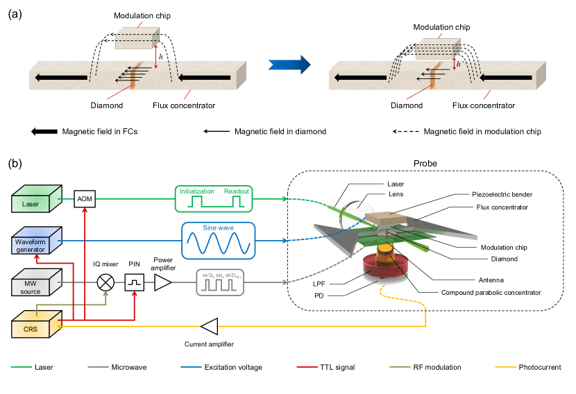
Fig. 2: Schematic of experimental setup. (a) Principle of FCM technique. Bold arrow, light arrow and dashed arrow represent for the magnetic field in FCs, in interval between FCs and in modulation chip, respectively. Thickness of arrow indicates the intensity of magnetic field. $h$ represents for the gap between modulation chip and FCs. With $h$ decreasing to $h^{\prime}$, the intensity of magnetic field in modulation chip increases, and the intensity of magnetic field in interval between FCs decreases conversely. (b) Experimental setups. CRS represents for home-built control and readout system. The CRS controls output of laser and microwave. The experiment is conducted by spin-echo sequence with $\pi/2-\pi-\pi/2$ microwave pulses. Waveform generator provides sinusoid signal for the excitation of piezoelectric bender. The output of the waveform generator is triggered by CRS. Dashed box on the right side is 3D rendering of the probe. LPF is low-pass filter. PD is photo diode. Fluorescence emitted from diamond is collected by a compound parabolic concentrator and finally detected by a PD. The photocurrent is recorded by CRS for analysis. Meanings of lines with different colors are shown below.

We utilized the mechanical motion scheme Tian2013 ; Edelstein2006 ; Guedes2008 to realize the FCM, as shown in Fig. 2(a). The mechanical motion scheme is implemented by a piezoelectric bender integrated with a modulation chip made of high permeability permalloy. The diamond sample is clamped by two Flux Concentrators (FCs). The modulation chip is placed on the top of the diamond sample and FCs. The FCs result in magnification of magnetic field on the diamond. The reduction of the gap $h$ leads to the decrease of magnetic field intensity in the diamond Tian2013 . Thus, with the periodically driven modulation chip, the magnetic field intensity in the diamond will become time-dependent. The external dc magnetic field can be modulated to an ac magnetic field, which has the same frequency as the driven signal, and it can be then detected by the NV magnetometry with spin-echo pulse sequence. This scheme provides a potential improvement in sensitivity by a factor of $\sqrt{T_{2}/T_{2}^{*}}$.

In our experiment, the resonant frequency of the piezoelectric bender is about 10.8 kHz with the load of modulation chip (See Sec. I in Supplementary Material). The maximum vibration amplitude of the piezoelectric bender is 3.6 $\rm\mu m$. We set the vibration amplitude to about 3 $\rm\mu m$ to avoid the overload of the bender. The amplitude corresponds to the modulation efficiency of 9.6% (See Sec. I in Supplementary Material).

Fig. 2(b) shows the schematic of this work. The optical system is composed of a 532 nm laser, a battery of lenses, and an Acoustic Optical Modulator (AOM) to generate initialization and readout laser pulses. The microwave system consists of a microwave (MW) source, an In-phase/Quadrature (IQ) mixer, a Positive-Intrinsic-Negative diode (PIN), and a power amplifier. Microwave from the MW source is multiplied with a radio-frequency (RF) signal fed into the IQ mixer. Then the output is gated by the PIN to generate the spin-echo sequence and amplified by a power amplifier. The MW signal is finally sent to a double split-ring microwave resonator Bayat2014 to drive the NV centers. The Control and Readout System (CRS) shown in the figure stands for a home-built system Qin2020 . Both of the AOM and the PIN timing is controlled by the Transistor-Transistor Logic (TTL) signals from the CRS. RF signals utilized to multiply with the MW signal are generated from the Arbitrary Waveform Generator (AWG) integrated into CRS. Another waveform generator provides a sinusoid signal for the excitation of a piezoelectric bender and it is also triggered by the CRS. Inside the probe, a couple of FCs is used to amplify the external magnetic field on the diamond. The length of FC is 4 cm and the width is 8 cm. The amplified magnetic field is modulated by a vibratory modulation chip glued onto the piezoelectric bender. The fluorescence is collected through a compound parabolic concentrator contacting one side of the diamond. After being separated from the excitation laser by a Long-Pass Filter (LPF), the fluorescence is transferred to the photodiode (PD). The signal from the PD are amplified by a current amplifier and finally sampled by the CRS. Another PD, which is not shown in this figure, is utilized to cancel the fluctuation of the laser’s intensity by monitoring the variation of the intensity of the laser as the reference signal Clevenson2015 ; Barry2017 .

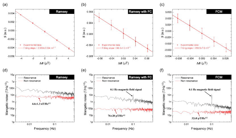
Fig. 3: Sensitivities of different methods. (a)-(c) The signal $S$ as the function of the applied magnetic fields for different methods. $S$ was obtained by the reference readout and the differential technique (See Sec. I in Supplementary Material). $\Delta B$ in abscissa represents for relative applied magnetic field. Four repetitive field-sweep spectra were tested. Each point on the figure was the average of four measurements. Error bars denote the standard deviation of four measurements. The maximum slope max$|\partial S/\partial B|$ was obtained from the fitting. (d)-(f) Magnetic field amplitude spectrum density of magnetometer based on different methods. The 0.1 Hz magnetic field signal was applied by coils for calibration. Green, blue and purple dashed lines represent for sensitivities of Ramsey protocol, Ramsey protocol with FC, and FCM method, respectively.

To demonstrate the enhancement of the sensitivities of NV-magnetometry, we carried out experiments to evaluate the sensitivities for three types of NV magnetometry. The first one is the Ramsey-type NV-magnetometry. The second one is Ramsey-type NV-magnetometry with FCs. Because of the magnification of the external magnetic field via FCs, the sensitivity of the second type of magnetometer is expected to be improved compared with first one without FCs. Both the sensitivities of the first and second types of magnetometry are limited by $T_{2}^{*}$. The third type is NV-magnetometry with FCM. The sensitivity of this type are expected to be further improved compared with the second one, and it is essentially limited by $T_{2}$. All the experiments were carried out with the same diamond in a magnetic shield.

We first measured the sensitivity of Ramsey-type NV-magnetometry. A coil was utilized to generate the external magnetic field, which is calibrated by a Tunnel MagnetoResistance (TMR) senor (See Sec. I in Supplementary Material). A stepped magnetic field generated by the coil was used to test the max$|\partial S/\partial B|$, as shown in the Fig. 3(a). The max$|\partial S/\partial B|$ of $0.959\pm 0.004$ mT^-1 was obtained. Then the time domain signal was measured by repeating the Ramsey sequence under resonance and non-resonance conditions, respectively. The non-resonance condition means that the microwave frequency was set to be far from the resonance frequency of the NV centers. The time domain signal with about one hour continuously acquisition was then converted to amplitude spectral density (ASD) Xie2021 to display the noise floor in frequency domain, as shown in the Fig. 3(d). The sampling rate for the acquisition was 1.15 Hz with one point accumulated by 4000 times. The ASD was computed using the Welch’s method with a 1380-point Blackman-Harris window with 50% overlap. The ASD measured under resonance condition was higher than the non-resonance condition. The thermal fluctuation caused by laser and MW is the the main reason to separate the two ASD spectra Fescenko2020 . To avoid this impact, previous works Jensen2014 ; Zheng2019 ; Zheng2020 using the ASDs measured under non-resonance conditions to evaluate the sensitivity of the NV-magnetometry. Due to the data rate limit of the acquisition system in the current setup, we met the challenge of increasing the sampling rate, so the estimated frequency range is from $\sim$0.003 Hz to $\sim$0.6 Hz in ASD. To estimate the magnetometry performance, we followed the previous works and used the non-resonant noise floor as the low-frequency sensitivity Jensen2014 ; Zheng2019 ; Zheng2020 , which was obtained as $4.6\pm 1.3$ nT/Hz^1/2 for Ramsey protocol in Fig. 3(d).

The experimental results of sensitivity of the Ramsey-type NV-magnetometry with FCs is shown in Fig. 3(b and e). The magnification of the external magnetic field via FCs is measured to be 85. As shown in the Fig. 3(b), the max$|\partial S/\partial B|$ with FCs was obtained as $68.3\pm 1.3$ mT^-1, which is about two orders of magnitude of that without FCs. The noise floors were also obtained as shown in the Fig. 3(e). The sensitivity of Ramsey-type NV-magnetometry with FCs is $76\pm 20$ pT/Hz^1/2.

The experimental results for sensitivity of NV-magnetometry with FCM are shown in Fig. 3(c and f). The vibration phase and the position of the modulation chip have been optimized (See Sec. I of Supplementary Material). As shown in the Fig. 3(c), the max$|\partial S/\partial B|$ of FCM method was $289.5\pm 7.6$ mT^-1. Due to the prolongation of $\tau$ with the FCM method, each data point was accumulated by 2000 times in order to maintain the same sampling rate of $\sim$1.15 Hz compared to the Ramsey experiment. The sensitivities of $32\pm 8$ pT/Hz^1/2 was obtained for FCM method.

A test signal with the frequency of 0.1 Hz was applied in all sensitivity tests (See Sec. I of Supplementary Material). In the measurement of Ramsey-type NV-magnetometry without FCs, there is no observation of such a signal. In the measurements of Ramsey-type NV-magnetometry with FCs and NV-magnetometry with FCM, there are clear observations of the test signal. It is clear that the signal to noise ratio of the test magnetic field by NV-magnetometry with FCM is much better than that from the Ramsey-type NV-magnetometry with FCs. We have successfully demonstrated the improvement of the sensitivity of dc NV-magnetometry by FCM.

To further investigate the potential of these methods, we establish a model according to previous works Barry2020 ; Degen2017 ; Xie2021 (See Sec. II in Supplementary Material) for the sensitivity evaluation as follows,

$$\eta\approx A\frac{n_{f}}{G\alpha E_{{}_{F}}\gamma_{e}e^{-\left(\tau/T_{\rm{coh}}\right)^{p}}C\sqrt{N}}\frac{\sqrt{t_{m}+\tau}}{\tau}\rm,$$ (1)

where $A$ is a coefficient for different pulse sequences. $A=1$ ($A=\pi/2$) is corresponding to the Ramsey protocol (spin-echo sequence) Barry2020 . $n_{f}$ is the ratio between overall noise of system and the shot noise. For the shot-noise limited sensitivity, we have $n_{f}=1$. $G$ is the magnification of FC. $\alpha$ is the angle factor used for describing the misalignment between magnetic field and the NV symmetry axis Xie2021 . $E_{{}_{F}}$ is modulation efficiency of the FCM method (See Sec. I of Supplementary Material). $\gamma_{e}$ is the gyromagnetic ratio of electron. $\tau$ is the evolution time of the NV center. $T_{\rm coh}$ is coherence time of the NV centers. $p$ is stretched exponential parameter depended on the origins of the dephasing Barry2020 . $C$ is the measurement contrast Taylor2008 . $N$ is the average number of photons detected per measurement. $t_{m}$ is the additional time in the pulse sequence (See Sec. II of Supplementary Material).

The parameters in the equation (4) can be experimentally measured as shown in table I in Supplementary Material. For the Ramsey-type NV-magnetometry without FCs, $G=1$ and $\tau=0.7~{}\rm\mu s$. The predicted sensitivity according to the equation (4) is 3.3 nT/Hz^1/2, which is consistent with the experimental result in Fig. 3(d). For the method of Ramsey-type NV-magnetometry by FC, the predicted sensitivity by equation (4) is 67 pT/Hz^1/2 with the parameters $G=85$ and $\tau=0.7~{}\rm\mu s$. The predicted sensitivity is also consistent with the experimental result. For the FCM method, $\tau$ has been set to $92.7~{}\rm\mu s$ to match the modulation frequency. The spin-echo sequence prolonged the coherence time, which was $102~{}\rm\mu s$ in Fig. 1(b). The experimental modulation efficiency of the FCM, $E_{{}_{F}}$, was 9.6%. The contrast C is 0.0045. With $T_{\rm coh}=T_{2}$, the predicted sensitivity of NV-magnetometry by FCM is 39 pT/Hz^1/2, which agrees with the experimental result. The slight differences between the evaluated sensitivities and the experimental values may come from the error of the parameters used in the evaluation. For example, the coefficient $A$ was not exactly $\pi/2$, since the modulated magnetic field was not a perfect sine. Nevertheless, the predicted sensitivities are consistent with the experimental results. Therefore, our model is suitable for predicting the performance of NV-magnetometry and we would like to utilize such model to evaluate the potential of sensitivity NV-magnetometry with FCM with current state-of-art technologies.

According to detailed evaluations in the Sec. II of Supplementary Material, the sensitivity can be further improved in the following steps by cutting-edge technologies. (i) When the width of the diamond is reduced, the magnification of the magnetic field by FCs can be increased. (ii) Through polishing modulation chip and FCs together with increasing vibration amplitude of piezoelectric bender, $E_{{}_{F}}$ can be increased to above fifty percent. This high modulation efficiency is achievable since a recent experiment reported a modulation efficiency up to 68.7% with a similar method Du2019 . (iii) The properties of the diamond can be further optimized. The coherence time can be improved with better diamonds together with advanced quantum control technologiesBauch2018 ; Wolf2015 . According to the detailed work on the diamond samples Barry2020 , $T_{2}$ is expected to be $\sim 700\ \rm\mu s$ with ¹²C enriched diamond, and the NV concentration of about 0.019 ppm is reachable. If the total internal reflection method Clevenson2015 is utilized, a reliable $N$ of $2.6\times 10^{10}$ with the above NV concentration is expected. (iv) The contrast $C$ in experiment is decreased by the inhomogeneity of the magnetic field in diamond. The inhomogeneity is mainly due to the FCs’ remanence as analyzed in the Supplementary Material. When such remanence of FCs is reduced via the demagnetization procedure, $C$ can be promoted to $\sim 1.2\times 10^{-2}$. With above improvements, an optimized shot-noise-limited sensitivity is expected to be $\sim 3~{}\rm fT/Hz^{1/2}$. Besides, the reduction of $n_{f}$ is essential on the way to the shot-noise-limited sensitivity, since it is about 20 in the current experiments. It could be helpful to improve the laser stability and reduce the noise of data acquisition system for decreasing $n_{f}$ Fescenko2020 ; Schloss2018 ; Chatzidrosos2017 . The further reduction of $n_{f}$ can lead to an achievable sensitivity of femtotesla level in the future study.

Our work demonstrates a dc quantum magnetometry with $T_{2}$-limited based on diamonds via flux modulation. Compared to the recent progress in dc NV-magnetometry via rotating the diamond, our method have a unique advantage as follows. Since FCM can be realized by Micro-ElectroMechanical Systems (MEMS), the power consumption and the size of the sensor can be further reduced. Very recently, a CMOS-integrated NV-Magnetometry has been successfully demonstrated Kim2019 . We further anticipate that a CMOS-integrated NV-Magnetometry with FCM by MEMS will provide a highly integrated low frequency magnetometry with high sensitivity. Our work provides a clear route towards femtotesla magnetometry at room temperature, which will play an important role in biological signal detection, such as magnetocardiography.

Supplementary Material

Appendix I Materials and methods

I.1 Sample preparation

The diamond sample used in this work was a single crystal chip (Element Six, DNV B1), grown by using chemical vapor deposition (CVD). Its typical initial nitrogen concentration and NV concentration were 0.8 ppm and 0.3 ppm, respectively. The diamond sample was cut into a piece with the size of 1.0 mm $\times$ 1.0 mm $\times$ 0.4 mm, and the 1.0 mm $\times$ 1.0 mm facet is perpendicular to $[100]$ crystal axis.

I.2 Probe with flux concentration and modulation

As shown in Fig. S1, the probe with Flux Concentration and Modulation (FCM) contains a commercial piezoelectric bender (Harbin Core Tomorrow, NAC2223), a modulation chip and two Flux Concentrators (FCs). The piezoelectric bender is a cuboid piezo-bimorph, whose size is 21.0 mm $\times$ 7.8 mm $\times$ 1.8 mm. Both end of the piezoelectric bender are glued onto an aluminium alloy holder. The modulation chip is a cuboid made of 1J85 alloy, whose size is 4 mm $\times$ 2 mm $\times$ 1 mm. The modulation chip is glued onto the center of piezoelectric bender. The size of the FCs is shown in Fig. S1. The FCs are specially shaped sheet metals made of 1J85 alloy. The thickness of FC is 1 mm.

The resonance frequency and the corresponding vibration amplitude of the piezoelectric bender were 10.795 kHz and 3.6 $\mu$m with the excitation voltage of 75 V, as shown in Fig. S1. In sensitivity tests, to protect the piezoelectric bender, the vibration amplitude was set to about 3.0 $\mu$m with the excitation voltage of 30 V. The vibration amplitude was tested by a high speed laser doppler vibrometer (Sunny Optical, LV-S01).

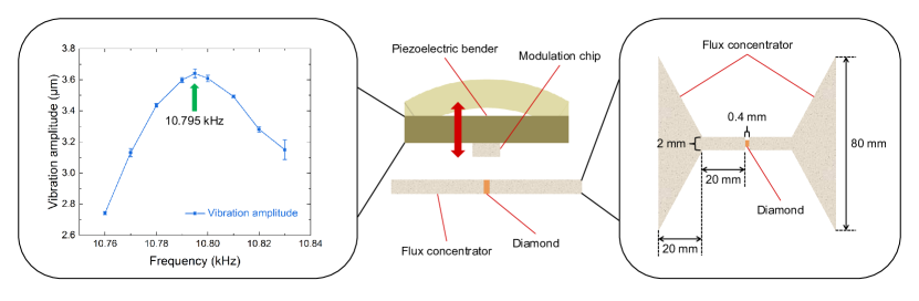
Fig. S1: Schematic of probe with FCM. The red double headed arrow indicates the vibration direction of piezoelectric bender. Black box on left side shows frequency-response curve of the piezoelectric bender. The frequency-response curve was obtained with the load of modulation chip. Black box on right side shows the size of FCs.

I.3 Position optimization of the modulation chip

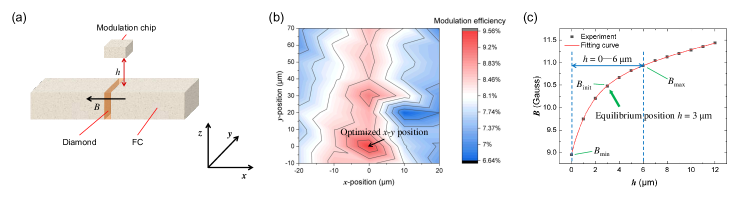
Fig. S2: Position optimization of the modulation chip. (a) Schematic of the modulation chip and the coordinate system. $h$ is the the minimum distance between modulation chip’s lower surface and FCs’ upper surface. $h=0$ means the two surfaces are in contact. (b) The x-y position optimization of the modulation chip. An optimal x-y position is indicated by the arrow. (c) $B$ as the function of $h$ measured at the optimal x-y position.

The position of the modulation chip should be optimized to achieve high modulation efficiency. The modulation efficiency $E_{{}_{F}}$, which is an important parameter for the sensitivity of FCM method, can be defined as pan12

$$E_{{}_{F}}=\frac{B_{\rm max}-B_{\rm min}}{2B_{\rm init}}\times 100\%.$$ (2)

$B_{\rm max}$ and $B_{\rm min}$ are maximum and minimum intensity of magnetic field in diamond clamped by FCs during the flux modulation. $B_{\rm init}$ is the intensity of magnetic field in diamond between FCs with modulation chip at the equilibrium position.

According to the equation (2), the optimized x-y position of the modulation chip can be achieved by changing $h$ and measuring $B$ at different x-y positions, denoted as B-h curve. The schematic of the FCM method and the coordinate system is shown in Fig. S2(a). A magnetic field of about 12.3 $\mu$T is applied during the optimization process. The magnetic field $B$ in diamond is obtained by measuring the resonance frequency extracted from the CW spectra. The optimization of the modulation chip’s x-y position is shown in Fig. S2(b). The irregular shape in Fig. S2(b) is due to the imperfect surfaces of the modulation chip and the FCs, discussied in Sec. II.3. Fig. S2(c) shows the B-h curve measured at the optimal x-y position shown in Fig. S2(b). $B$ decreases with $h$ decreasing. Since the vibration amplitude of piezoelectric bender is set to 3 $\mu$m, the equilibrium position of modulation chip is chosen as $h=3~{}\mu$m to achieve maximal modulation efficiency. $B_{\rm max}=$ 10.95 Gauss, $B_{\rm min}=$ 8.95 Gauss and $B_{\rm init}=$ 10.47 Gauss with above configuration are indicated on the Fig. S2(c). Thus $E_{{}_{F}}=9.6$% is obtained by using (2).

I.4 Vibration phase optimization of the piezoelectric bender

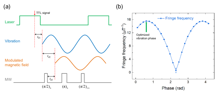
Fig. S3: Vibration phase optimization of the piezoelectric bender. (a) Spin-echo sequence and modulated magnetic field. (b) The frequency of the fringe as the function of the relative vibration phase. The phase is calculated by the trigger time of TTL signal. The optimal vibration phase is indicated by green arrow on the figure. The frequency of the fringe is obtained by fitting with sine function.

Fig. S3(a) defines three delay times. $t_{d1}$ is the delay time between a Transistor-Transistor Logic (TTL) signal and the beginning of piezoelectric bender vibration. $t_{d2}$ is the delay time between the beginning of piezoelectric bender vibration and the equilibrium point of the modulated magnetic field. The equilibrium point is defined as the intensity of the modulated magnetic field equivalent to $B_{\rm init}$. $t_{d3}$ is the delay time between the equilibrium point of the modulated magnetic field and the ending of the first $\pi/2$-pulse in the spin-echo sequence. The vibration phase of the piezoelectric bender is depended on the three delay times, compared to the first $\pi/2$-pulse in the spin-echo sequence.

$t_{d3}$ is essential for the spin-echo magnetometry. Since the three delay times are fixed, we optimize $t_{d3}$ by changing the trigger time of the TTL signal. To obtained the optimal sensitivity, we measured the fringe of the signal $S$ as the function of an applied static magnetic field under the different TTL signal delay, and calculated the frequency of the fringe. In experiment, a TTL signal was sent to waveform generator to trigger piezoelectric bender’s vibration. Fig. S3(b) shows the vibration phase optimization of piezoelectric bender. The abscissa was calculated from the trigger time divided the vibration period. The optimized trigger time for an optimal vibration phase was obtained with the optimization.

I.5 Experimental setup

The 532-nm laser was provided by a high-power optically pumped semiconductor laser (Coherent, Verdi G5). The microwave was generated by a microwave frequency synthesizer (National Instrument, FSW-0010). The IQ mixer (Marki, MLIQ0218L), the PIN (Mini-Circuits, ZASWA-2-50DRA+), the customized 20 W power amplifier and the double split-ring microwave resonator were used for microwave pulse sequence generation. The piezoelectric bender was driven by a waveform generator (RIGOL, DG812). The home-built CRS based on Field-Programmable Gate Array (FPGA) was used to generate TTL signals to AOM (ISOMET, M1133-aQ80L-1.5), PIN and the waveform generator. The RF modulation signal, generated by CRS, was applied to IQ mixer. The fluorescence was detected by a PD (Thorlabs, SM05PD1A) after collected by a compound parabolic concentrator (Edmund Optics, #65-441). The photocurrent was amplified by a current amplifier (FEMTO, DHPCA-100) and finally sampled by the CRS.

I.6 Experimental method

The external magnetic field was applied by a coil placed near the probe. The coil’s conversion coefficient of 4.1 $\mu$T/V was obtained using a Tunnel Magnetoresistance (TMR) magnetometer (MultiDimension Technology, USB27053). The 0.1 Hz test signal in sensitivity measurements was applied by another coil via the 0.1 Hz alternating voltage fed into it. The intensity of the test signal was 12 nT. The probe and coils for applying magnetic field were placed in a magnetic shield. All the experiments were performed under the magnetic shielding condition.

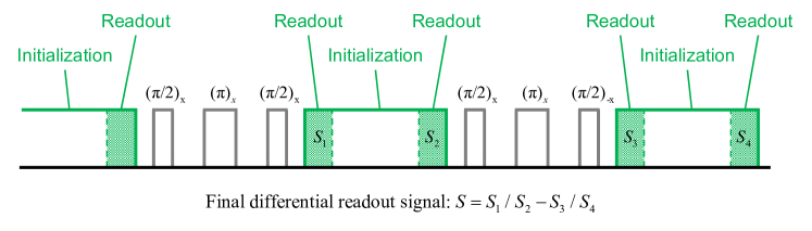
Fig. S4: Spin-echo sequence and the readout procedure used in this work. $S_{1}$, $S_{2}$, $S_{3}$ and $S_{4}$ represents the integrated signal in the specified readout duration, respectively. The final differential readout signal $S$ can be obtained as $S=S_{1}/S_{2}-S_{3}/S_{4}$.

The readout procedure used in this work are shown by Fig. S4. The laser pulse in the spin-echo sequence contained the initialization duration and the readout duration. The intensity of the optical signal was recorded in readout duration. A laser pulse contained one initialization duration and two readout durations. Data acquired in the first readout duration was divided by data acquired in second readout duration for normalization.

To suppress common mode noise, another differential method was used. In experiment, the first microwave pulse sequence $(\pi/2)_{x}-(\pi)_{x}-(\pi/2)_{x}$ and the second microwave pulse sequence $(\pi/2)_{x}-(\pi)_{x}-(\pi/2)_{-x}$ were played alternately. The second microwave pulse sequence was realized by reversing the phase of the second $\pi/2$ pulse. Signal acquired from the first microwave pulse sequence was subtracted by the signal of the second microwave pulse sequence to suppress the common mode noise.

Appendix II Further sensitivity improvement

II.1 Magnetic field sensitivity

The shot-noise-limited magnetic field sensitivity of the spin-echo protocol can be defined as Barry2020 ; Degen2017

$$\eta_{\rm spin-echo}^{\rm shot}\approx\frac{\pi}{2}\frac{\hbar}{\Delta m_{s}g_{e}\mu_{B}}\frac{1}{e^{-\left(\tau/T_{2}\right)^{p}}C\sqrt{N}}\frac{\sqrt{t_{I}+\tau+t_{r}}}{\tau}$$ (3)

where $\pi/2$ is corresponding to the spin-echo protocol Barry2020 . $\hbar$ is reduced Planck constant. $\Delta m_{s}$ is the difference in spin quantum number between the two interferometry states. $g_{e}$ is the Landég-factor of electron spin. $\mu_{B}$ is Bohr magneton. $\tau$ is the evolution time of the NV center. $T_{2}$ is coherence time of the NV center. $p$ is stretched exponential parameter depended on the origins of the dephasing Barry2020 . $C$ is the measurement contrast Barry2020 . $N$ is the average number of photons detected per measurement. $t_{I}$ and $t_{r}$ are the duration of initialization and readout respectively.

We set $\gamma_{e}={\hbar}/{g_{e}\mu_{B}}$ and $t_{m}=t_{r}+t_{I}+t_{d}$ for simplifying the equation (3). $t_{d}$ is the multiple time delays in pulse sequence with minor contribution to $t_{m}$. To match different types of NV-magnetometry, the coefficient ${\pi}/{2}$ is replaced by $A$, and the coherence time $T_{2}$ is replaced by $T_{\rm coh}$. $A=1$ ($A=\pi/2$) is corresponding to the Ramsey protocol (spin-echo protocol) Barry2020 . According to the previous work of the flux concentration Xie2021 , we add the the magnification $G$ of FC and the angle factor $\alpha$. The modulation of the magnetic field introduces a new parameter $E_{{}_{F}}$ pan12 , defined in the equation (2). For the Ramsey-type magnetometry, we have $E_{{}_{F}}=1$ since the external magnetic field is not modulated. Because the system noise must be larger than the shot noise, we define $n_{f}$ as the ratio between overall system noise and the shot noise. With the above preconditions, the equation (3) can be rewritten as

$$\eta\approx A\frac{n_{f}}{G\alpha E_{{}_{F}}\gamma_{e}e^{-\left(\tau/T_{\rm coh}\right)^{p}}C\sqrt{N}}\frac{\sqrt{t_{m}+\tau}}{\tau}\rm,$$ (4)

where $\alpha$ is the angle factor used for describing the misalignment between magnetic field and the NV symmetry axis Xie2021 . For the shot-noise limited sensitivity, we have $n_{f}=1$. $\gamma_{e}$ is the gyromagnetic ratio of electron. $T_{\rm coh}$ is coherence time of the NV centers.

According to the experimental data, the parameters of three methods in equation (4) are shown in Table 1. The $p=1$ is used for the Ramsey-type magnetometry Barry2020 . From the equation (4), the duty cycle ${{\tau}}/({t_{m}+\tau})$ is also important for the sensitivity enhancement. From Table 1, we know the duty cycle increase from $<1\%$ to $\sim 40\%$. The NV-magnetometry with FCM gives a sensitivity enhancement of 140 folds compared to the Ramsey-type NV-magnetometry.

Table 1: Parameters used in the sensitivity evaluations

Parameter	Ramsey	Ramsey with FC	FCM
$A$	1	1	$\pi$/2
$G$	1	85.1	85.1
$E_{{}_{F}}$	1	1	0.096
$N$	7.6 $\times$ 109	7.0 $\times$ 109	7.0 $\times$ 109
$C$	1.2 $\times$ 10-2	9.2 $\times$ 10-3	4.5 $\times$ 10-3
$T_{\rm coh}$	1.13 $\mu$s	1.13 $\mu$s	102 $\mu$s
$\tau$	0.7 $\mu$s	0.7 $\mu$s	92.7 $\mu$s
$t_{m}$	115 $\mu$s	115 $\mu$s	140 $\mu$s
$n_{f}$	12.2	15.6	19.2
$p$	1	1	1.24
$\gamma_{e}$	2$\pi$ $\times$ 28 GHz/T	2$\pi$ $\times$ 28 GHz/T	2$\pi$ $\times$ 28 GHz/T
$\alpha$	0.5774	0.5774	0.5774
$\eta$ (Experiment)	4.6 nT/Hz1/2	76 pT/Hz1/2	32 pT/Hz1/2
$\eta$ (Evaluation)	3.3 nT/Hz1/2	67 pT/Hz1/2	39 pT/Hz1/2

II.2 Improvement of the magnification ($G$)

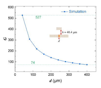
Fig. S5: The simulation magnification as the function of the gap width $d$ with the modulation chip nearby. Noticed that a modulation chip exists in the simulation. $h$ is set to 40.4 $\mu$m. The impact of the imperfect modulation chip will be discussed in the section II.3.

The magnification $G$ is decided by the geometry of FCs and the gap width between FCs Xie2021 . Considering the future applications in biomagnetism, we only optimize the gap between FCs to increase $G$. In experiment, the gap width is 0.4 mm, which is the thickness of the diamond sample. Diameter of the laser spot on diamond is about 40 $\mu$m. So the minimum gap width between FCs can be reduced to 40 $\mu$m by thinning diamond sample.

The simulation magnification as the function of the gap width $d$ are shown in Fig. S5. The magnification of the FCs increases rapidly with the decrease of $d$. According to the simulation result, the magnification increases from 74 to 527 with the gap width reducing from 0.4 mm to 40 $\mu$m.

II.3 Improvement of the modulation efficiency ($E_{{}_{F}}$)

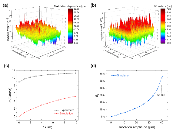
Fig. S6: The surface morphology and the modulation efficiency. (a)-(b) The surface morphology of the modulation chip and the FCs, respectively. The relative height is measured by a position sensor and subtracted by minimum relative height for a clear view. (c) The magnetic field in diamond versus $h$. The simulation is conducted by assuming the ideal configuration of the modulation chip and the FCs, which are perfectly parallel and smooth. (d) The modulation efficiency as the function of the vibration amplitude. The equilibrium position of the modulation chip is set as $h=$ 40.4 $\mu$m in the simulation.

$E_{{}_{F}}$ is affected by the gap width between the modulation chip and the FCs. In experiment, the surfaces of modulation chip and FCs are rough. The surface roughness of the modulation chip and the FCs are shown in Fig. S6(a) and Fig. S6(b). According to the figures, the surface roughness of modulation chip and FC are larger than 30 $\mu$mRz and 7 $\mu$mRz, respectively. In experiment, the width of gap $h$ is the minimum distance between modulation chip’s lower surface and FCs’ upper surface. Fig. S6(c) shows the results of the magnetic field in diamond between FCs as the function of $h$. The simulation result in Fig. S6(c) is an ideal configuration of the modulation chip and the FCs. It is noted that $h=0$ (simulation) corresponds to the perfect contact of the modulation chip and the FCs, which leads to the magnetic field intensity in diamond of nearly zero.

The other key parameter, which has the impact on the modulation efficiency, is the vibration amplitude of piezoelectric bender. $B_{\rm max}$ and $B_{\rm min}$ in (2) are decided by vibration amplitude as shown in Fig. S2(d). Fig. S6(d) shows the modulation efficiency as the function of the vibration amplitude. In Fig. S6(d), the equilibrium position of modulation chip is set as $h=$ 40.4 $\mu$m. With the vibration amplitude reaching 40.4 $\mu$m, the modulation efficiency of 56.8$\%$ can be achieved.

According to the above discussion, the following methods can enhance the modulation efficiency. The first one is polishing of the modulation chip and the FCs, and second one is improving the vibration amplitude of the piezoelectric bender. The polishing of the modulation chip and the FCs enables the perfect contact of the two objects. The electron beam uno07 and micron-sized diamonds kubota20 could be used to reduce the surface roughness of the two objects to several nanometers. Under the same excitation voltage, the product of the vibration amplitude and the resonance frequency of the piezoelectric bender can be an approximate invariant, depended on piezoelectric coefficients and quality factor wang98 . PZT8 is a low damping piezoelectric material with high piezoelectric coefficients $d_{13}$ of 240 pC/N. As a reference, a piezoelectric bender is fabricated by cuboid cut PZT8 fastened to silicon substrate via Au-In metal bonding and realized resonance frequency over 8 kHz with vibration amplitude about 15 $\mu$m du19 . Thus a piezoelectric bender with the resonance frequency over 3 kHz and the vibration amplitude over 40 $\mu$m can be achievable by using PZT8. With the above improvements, the modulation efficiency about 56.8$\%$ can be achieved according the simulation as shown in Fig. S6(d).

II.4 Improvement of the coherence time ($T_{\rm coh}$)

For the NV-magnetometry with FCM, the coherence time $T_{2}$ is regarded as $T_{\rm coh}$. Due to the low applied magnetic field in this work, no ¹³C revival was obtained as shown in Fig. 1(a) of main text. Under the applied magnetic field of low strength, the natural abundance of ¹³C decrease $T_{2}$. With ¹²C enrich technique, the effect of ¹³C can be suppressed Bauch2020 .

According to the detailed work on diamond samples Barry2020 ; Bauch2018 , the expected $T_{2}$ of $\sim$700 $\mu$s is achievable with the nitrogen concentration of about 0.05 ppm. The nitrogen-to-NV conversion efficiency of the diamond used in this work is about 37.5% (Element Six, DNV B1). The NV concentration of 0.019 ppm is reachable for the nitrogen concentration of about 0.05 ppm in the future.

II.5 Improvement of the average number of photons detected per measurement ($N$)

The number $N$ is depended on the photoluminescence rate $R$ of single NV center and the the number of the NV centers being excited. $R$ can be estimated as Chapman2011

$$R=R_{\infty}(k)\frac{I}{I+I_{s}(\sigma,k)},$$ (5)

where $R_{\infty}$ is maximum detected photoluminescence rate of single NV center. $I$ is the power density of the laser. $I_{s}$ is saturation intensity of the laser. Because of the NV centers’ absorption to laser, $I=I_{0}e^{-\beta L}$ decreases with the path length $L$ of excitation laser, where $I_{0}$ is the incident power density of the laser. $\beta$ is the absorption coefficient for the laser. The absorption cross-section $\sigma_{\rm NV}$ of NV center is about 1 $\times$ 10^-16 cm² Chapman2011 . Thus, $N$ can be estimated by the integral of $R$ for all NV centers being excited in the laser, and we have

$$N\approx\int_{0}^{L_{\rm max}}Rt_{r}n_{{}_{\rm NV}}\pi r^{2}dL,$$ (6)

where $L_{\rm max}$ is the maximum path length of the excitation laser in the diamond. $t_{r}$ is the readout time per measurement. $n_{\rm NV}$ is the concentration of the NV centers in diamond. $r$ is the radius of the laser spot.

In this work, the laser power was 0.375 W. $t_{r}$ was 9 $\mu$s. $r$ was 20 $\mu$m. The area of the laser spot was about $1.3\times 10^{3}$ $\mu$m². $n_{\rm NV}$ was about 0.3 ppm. The attenuation coefficient $\beta=\sigma_{\rm NV}n_{\rm NV}$ was 528 m^-1. $L_{\rm max}$ was 1 mm for the single-pass configuration. According to the experiment, the fluorescence intensity is about 0.22 mW. The average wavelength of the fluorescence is 680 nm. To fit the experimental result, $R_{\infty}=44.8$ kHz is obtained with the assumption of $I_{s}=650$ MW/m² plakhotnik10 . Thus $N$ is calculated as 7.0 $\times$ 10⁹.

To improve $N$, we are going to use the total internal reflection Clevenson2015 to increase the number of the NV centers being excited. With $n_{\rm NV}$ of 0.019 ppm in the future, we have the attenuation coefficient $\beta=\sigma_{\rm NV}n_{\rm NV}$ of 33.44 m^-1. $L_{\rm max}$ will be $\sim$32 mm, while the whole diamond with the size of 0.04 mm $\times$ 1 mm $\times$ 1 mm is excited. According to the simulation result, the collection efficiency can be enhanced by 2.2 folds with the coating technique yu20 and a better fabrication technique of diamond and CPC. Thus $R_{\infty}$ of 98.6 kHz is available with the improvements. It should be noticed that a long-pass dielectric film is required to prevent the intensity loss of the laser. The dielectric film should be able to reflect the laser, and coated on the diamond surface contacted with CPC. To avoid effects on other parameters, we do not change the laser power and the diameter of the laser spot in the calculation. With $I_{s}=650$ MW/m² plakhotnik10 and $R_{\infty}=98.6$ kHz, the $N$ can be improved from 7.0 $\times$ 10⁹ to 2.6 $\times$ 10¹⁰.

II.6 Improvement of the measurement contrast ($C$)

For the Ramsey-type NV-magnetometry, $C$ was about 1.2$\times$10^-2. For the NV-magnetometry with FCM, $C$ was about 4.5$\times$10^-3. The decrease mainly comes from the magnetic field inhomogeneity in diamond. We describe a model for the impact of the magnetic field inhomogeneity. The signal of the magnetometry based on the ensemble of NV centers can be represented as

$$S=\int dG^{\prime}\int dB_{r}P_{0}(G^{\prime})P_{1}(B_{r})S^{\prime}(B),$$ (7)

where $B=G^{\prime}B_{a}+B_{r}$ is the magnetic field acting on the NV centers, and $S^{\prime}(B)$ is the readout signal of the NV centers under $B$. $G^{\prime}$ is the magnification of the FCs for $B_{a}$. $B_{a}$ is the applied magnetic field to the probe. $B_{r}$ is a static magnetic field, which could come from the remanence of the FCs. $P_{0}(G^{\prime})$ and $P_{1}(B_{r})$ are the distributions of the parameters.

According to previous discussions in the solid-state spins Bauch2020 ; Rong2015 ; Boss2017 , we suppose that $P_{0}(G^{\prime})$ and $P_{1}(B_{r})$ are satisfied with the widely used normal distribution. Thus the two distributions are characterized as

$$\begin{cases}P_{0}(G^{\prime})&=\frac{1}{\sqrt{2\pi}kG}exp\left[-\frac{(G^{\prime}-G)^{2}}{2(kG)^{2}}\right]\\ P_{1}(B_{r})&=\frac{1}{\sqrt{2\pi}mB_{r0}}exp\left[-\frac{(B_{r}-B_{r0})^{2}}{2(mB_{r0})^{2}}\right]\\ \end{cases}$$ (8)

where $k$ and $m$ are relative scale parameters of the corresponding distributions. $G$ and $B_{r0}$ are mean values of the corresponding distributions.

Fig. S7: The simulation of $C$ under different conditions. (a) The signal as the function of $B_{a}$ under different $k$. Factor $m$ was set to be 0.01 in the simulation. (b) The signal as the function of $B_{a}$ under different $m$. Factor $k$ was set to be 0.01 in the simulation. (c) The comparison between the experiment and the simulation. In the simulation with the practical condition, $k$ and $m$ were set to be 0.015 and 0.109, respectively. In the simulation with the ideal condition, $k$ and $m$ were both set to be 0.01. (d) The simulation result of $C$ as the function of the averaged remanence of the FCs $B_{r0}$. $k$ and $m$ were set to be 0.015 and 0.109 as in the simulation of the practical condition.

The simulation is performed by changing applied magnetic field $B_{a}$. Fig. S7(a) and Fig. S7(b) show the signal as the function of $B_{a}$ with different $k$ and $m$, respectively. The contrast of the signal decreases with factor $k$ increasing at the large $B_{a}$. The holistic decrease of the contrast can be observed with the increase of $m$. It can be summarized as that the stronger magnetic field inhomogeneity leads to the larger decrease of $C$.

To match with the experimental data, we adjust $k$ and $m$. Fig. S7(c) shows the comparison between the experiment and the simulation, which is perfectly matching. It should be noticed that the spectra is not symmetry about $B_{a}=0$ due to $B_{r0}$. All the parameters used in the simulation are listed in Table 2.

According to the above simulations, the reduction of FC’s remanence is helpful in the improvement of $C$. Fig. S7(d) shows the simulation result of $C$ as the function $B_{r0}$. To increase $C$ to about 1.2$\times$10^-2, we have to suppress $B_{r0}$ to less than 2 $\mu$T from Fig. S7(d). The elimination of FC’s remanence can be realized by applying an ac magnetic field to the FC gerdroodbari18 .

Table 2: Parameters used in simulation for Fig. S7(c)

Parameter	Value	Parameter	Value
$k$	0.015 (practical) / 0.01 (ideal)	$G$	85.1
$m$	0.109 (practical) / 0.01 (ideal)	$B_{r0}$	25.0 $\mu$T
$C$	1.2 $\times$ 10-2	$T_{2}$	102 $\mu$s
$p$	1.24	$\tau$	92.7 $\mu$s

II.7 The potentially achievable sensitivity

According to the above discussions, the shot-noise-limited sensitivity of the NV-magnetometry with FCM can reach $\sim$3 fT/Hz^1/2, evaluated by the equation (4). For an achievable $n_{f}$ of 3, the sensitivity of femtotesla level is promising. All the parameters used in the evaluation are listed in Table 3.

From Table 3, we can see the essential enhancements coming from the magnification $G$ of the FCs, the modulation efficiency $E_{{}_{F}}$, and the noise ratio $n_{f}$. The improvements of $G$ and $E_{{}_{F}}$ require the micromachining technologies. The improvement of $n_{f}$ requires further efforts on the readout system optimization. Although a sensitivity of femtotesla level is proposed, more efforts on the excitation and the quantum sensing protocols could lead to a more promising result. This $T_{2}$-limited dc quantum magnetometry is worth further exploration.

Table 3: Parameters used in sensitivity calculation.

Parameter	Present value	Improved value	Enhancement for sensitivity	Reference
$G$	85.1	527	6.2	Simulation
$E_{{}_{F}}$	0.096	0.568	5.9	uno07 , kubota20 , du19 , Simulation
$T_{2}$	102 $\mu$s	$\sim$ 694 $\mu$s	$\sim$ 1.6	Bauch2020
$N$	7.0 $\times$ 109	2.6 $\times$ 1010	1.9	Clevenson2015 , yu20
$C$	4.5 $\times$ 10-3	$\sim$ 1.2 $\times$ 10-2	$\sim$ 2.7	gerdroodbari18 , Simulation
$\tau$	92.7 $\mu$s	333.6 $\mu$s	2.5	Experiment
$t_{m}$	140 $\mu$s	140 $\mu$s	$/$	Experiment
$n_{f}$	19.2	19.2	$/$	Experiment
$p$	1.24	1.24	$/$	Experiment
$\gamma_{e}$	2$\pi$ $\times$ 28 GHz/T	2$\pi$ $\times$ 28 GHz/T	$/$	$/$
$\alpha$	0.5774	0.5774	$/$	$/$
$\eta$ (Evaluation)	39 pT/Hz1/2	$\sim$ 50 fT/Hz1/2	$\sim$ 750.6	Calculation
$\eta$ (Shot-noise-limited)	2 pT/Hz1/2	$\sim$ 3 fT/Hz1/2	$\sim$ 750.6	Calculation

References

- (1) E. Boto, et al., Moving magnetoencephalography towards real-world applications with a wearable system. Nature 555, 657 (2018).
- (2) D. Cohen, Magnetic Fields around the Torso: Production by Electrical Activity of the Human Heart. Science 156, 652 (1967).
- (3) J. Lenz, S. Edelstein, Magnetic sensors and their applications. IEEE Sensors Journal 6, 631 (2006).
- (4) D. R. Glenn, et al., Micrometer-scale magnetic imaging of geological samples using a quantum diamond microscope. Geochemistry, Geophysics, Geosystems 18, 3254 (2017).
- (5) M. Jiao, M. Guo, X. Rong, Y.-F. Cai, J. Du, Experimental Constraint on an Exotic Parity-Odd Spin- and Velocity-Dependent Interaction with a Single Electron Spin Quantum Sensor. Physical Review Letters 127, 010501 (2021).
- (6) C. L. Degen, F. Reinhard, P. Cappellaro, Quantum sensing. Reviews of Modern Physics 89, 1 (2017).
- (7) D. Budker, M. Romalis, Optical magnetometry. Nature Physics 3, 227 (2007).
- (8) C. Dolabdjian, D. Menard, A. Grosz, M. J. Haji-Sheikh, S. C. Mukhopadhyay, High Sensitivity Magnetometers, vol. 19 of Smart Sensors, Measurement and Instrumentation (Springer International Publishing, Cham, 2017).
- (9) J. M. Taylor, et al., High-sensitivity diamond magnetometer with nanoscale resolution. Nature Physics 4, 810 (2008).
- (10) K. Jensen, et al., Cavity-Enhanced Room-Temperature Magnetometry Using Absorption by Nitrogen-Vacancy Centers in Diamond. Physical Review Letters 112, 160802 (2014).
- (11) G. Chatzidrosos, et al., Miniature Cavity-Enhanced Diamond Magnetometer. Physical Review Applied 8, 044019 (2017).
- (12) H. Clevenson, et al., Broadband magnetometry and temperature sensing with a light-trapping diamond waveguide. Nature Physics 11, 393 (2015).
- (13) Y. Xie, et al., A hybrid magnetometer towards femtotesla sensitivity under ambient conditions. Science Bulletin 66, 127 (2021).
- (14) I. Fescenko, et al., Diamond magnetometer enhanced by ferrite flux concentrators. Physical Review Research 2, 023394 (2020).
- (15) C. Zhang, et al., Diamond Magnetometry and Gradiometry Towards Subpicotesla dc Field Measurement. Physical Review Applied 15, 064075 (2021).
- (16) F. Barry, et al., Optical magnetic detection of single-neuron action potentials using quantum defects in diamond. Proceedings of the National Academy of Sciences 114, E6730 (2017).
- (17) J. F. Barry, et al., Sensitivity optimization for NV-diamond magnetometry. Reviews of Modern Physics 92, 015004 (2020).
- (18) E. Bauch, et al., Ultralong Dephasing Times in Solid-State Spin Ensembles via Quantum Control. Physical Review X 8, 031025 (2018).
- (19) T. Wolf, et al., Subpicotesla Diamond Magnetometry. Physical Review X 5, 041001 (2015).
- (20) Y.-X. Liu, A. Ajoy, P. Cappellaro, Nanoscale Vector dc Magnetometry via Ancilla-Assisted Frequency Up-Conversion. Physical Review Letters 122, 100501 (2019).
- (21) A. A. Wood, et al., T2-limited sensing of static magnetic fields via fast rotation of quantum spins. Physical Review B 98, 174114 (2018).
- (22) E. L. Hahn, Spin echoes. Phys. Rev. 80, 580 (1950).
- (23) W. Tian, J. Hu, M. Pan, D. Chen, J. Zhao, Flux concentration and modulation based magnetoresistive sensor with integrated planar compensation coils. Review of Scientific Instruments 84, 035004 (2013).
- (24) A. S. Edelstein, et al., Progress toward a thousandfold reduction in 1/f noise in magnetic sensors using an ac microelectromechanical system flux concentrator (invited). Journal of Applied Physics 99, 08B317 (2006).
- (25) A. Guedes, et al., Hybrid magnetoresistive/microelectromechanical devices for static field modulation and sensor 1/f noise cancellation. Journal of Applied Physics 103, 1 (2008).
- (26) K. Bayat, J. Choy, M. Farrokh Baroughi, S. Meesala, M. Loncar, Efficient, Uniform, and Large Area Microwave Magnetic Coupling to NV Centers in Diamond Using Double Split-Ring Resonators. Nano Letters 14, 1208 (2014).
- (27) X. Qin, et al., An fpga-based hardware platform for the control of spin-based quantum systems. IEEE Transactions on Instrumentation and Measurement 69, 1127 (2020).
- (28) H. Zheng, et al., Zero-Field Magnetometry Based on Nitrogen-Vacancy Ensembles in Diamond. Physical Review Applied 11, 064068 (2019).
- (29) D. Zheng, et al., A hand-held magnetometer based on an ensemble of nitrogen-vacancy centers in diamond. Journal of Physics D: Applied Physics 53, 155004 (2020).
- (30) Q. Du, et al., High Efficiency Magnetic Flux Modulation Structure for Magnetoresistance Sensor. IEEE Electron Device Letters 40, 1824 (2019).
- (31) J. M. Schloss, J. F. Barry, M. J. Turner, R. L. Walsworth, Simultaneous Broadband Vector Magnetometry Using Solid-State Spins. Physical Review Applied 10, 034044 (2018).
- (32) D. Kim, et al., A CMOS-integrated quantum sensor based on nitrogen–vacancy centres. Nature Electronics 2, 284 (2019).
- (33) M. Pan, J. Hu, W. Tian, D. Chen, J. Zhao, Magnetic flux vertical motion modulation for 1/f noise reduction of magnetic tunnel junctions. Sensors and Actuators A: Physical 179, 92 (2012).
- (34) Y. Uno, et al., A new polishing method of metal mold with large-area electron beam irradiation. Journal of Materials processing technology 187, 77 (2007).
- (35) A. Kubota, S. Nagae, S. Motoyama, High-precision mechanical polishing method for diamond substrate using micron-sized diamond abrasive grains. Diamond and Related Materials 101, 107644 (2020).
- (36) Q.-M. Wang, L. E. Cross, Performance analysis of piezoelectric cantilever bending actuators. Ferroelectrics 215, 187 (1998).
- (37) Q. Du, et al., High efficiency magnetic flux modulation structure for magnetoresistance sensor. IEEE Electron Device Letters 40, 1824 (2019).
- (38) E. Bauch, et al., Decoherence of ensembles of nitrogen-vacancy centers in diamond. Physical Review B 102, 134210 (2020).
- (39) R. Chapman, T. Plakhotnik, Quantitative luminescence microscopy on Nitrogen-Vacancy Centres in diamond: Saturation effects under pulsed excitation. Chemical Physics Letters 507, 190 (2011).
- (40) T. Plakhotnik, D. Gruber, Luminescence of nitrogen-vacancy centers in nanodiamonds at temperatures between 300 and 700 k: perspectives on nanothermometry. Physical Chemistry Chemical Physics 12, 9751 (2010).
- (41) H. Yu, Y. Xie, Y. Zhu, X. Rong, J. Du, Enhanced sensitivity of the nitrogen-vacancy ensemble magnetometer via surface coating. Applied Physics Letters 117, 204002 (2020).
- (42) X. Rong, et al., Experimental fault-tolerant universal quantum gates with solid-state spins under ambient conditions. Nature Communications 6, 8748 (2015).
- (43) J. M. Boss, K. S. Cujia, J. Zopes, C. L. Degen, Quantum sensing with arbitrary frequency resolution. Science 356, 837 (2017).
- (44) Y. Z. Gerdroodbari, M. Davarpanah, S. Farhangi, Remanent flux negative effects on transformer diagnostic test results and a novel approach for its elimination. IEEE Transactions on Power Delivery 33, 2938 (2018).