LaMemo: Language Modeling with Look-Ahead Memory

Abstract

Although Transformers with fully connected self-attentions are powerful to model long-term dependencies, they are struggling to scale to long texts with thousands of words in language modeling. One of the solutions is to equip the model with a recurrence memory. However, existing approaches directly reuse hidden states from the previous segment that encodes contexts in a uni-directional way. As a result, this prohibits the memory to dynamically interact with the current context that provides up-to-date information for token prediction. To remedy this issue, we propose Look-Ahead Memory (LaMemo) that enhances the recurrence memory by incrementally attending to the right-side tokens, and interpolating with the old memory states to maintain long-term information in the history. LaMemo embraces bi-directional attention and segment recurrence with an additional computation overhead only linearly proportional to the memory length. Experiments on widely used language modeling benchmarks demonstrate its superiority over the baselines equipped with different types of memory.

1 Introduction

Language modeling is an important task that tests the ability of modeling long-term dependencies by predicting the current token based on the previous context (Mikolov and Zweig, 2012; Merity et al., 2017). Recently, Transformer-based language models achieved remarkable performance by enabling direct interaction between long-distance word pairs. However, as the computation overhead grows with the length of the input sequence, Transformers can only process a fixed length segment at a time. To allow long-term information flow across individual segments, existing approaches augment the model with a recurrence memory that stores hidden states computed in previous time steps (Dai et al., 2019) and their compressions (Rae et al., 2020; Martins et al., 2021) for the target tokens to attend to.

One limitation of this approach is that the recurrence memory is only aware of older contexts since they are previously computed to predict the next word from left to right. As a result, distant memory states become outdated and less activated by the current context, as illustrated in Figure 1. When humans read or write a document, they maintain a memory that records important information from the past and often refresh them under the current context to keep it up-to-date.

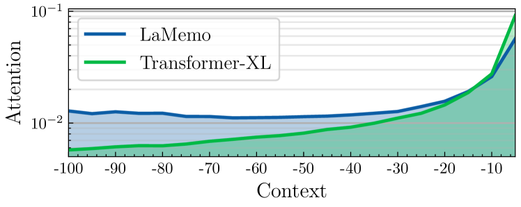
Figure 1: Attention weights on the context (in log-scale) in the final layer of Transformer-XL and LaMemo averaged on 15K tokens. Transformer-XL quickly loses attention to older contexts, while LaMemo maintains awareness to the history with the grow of the context length.

In this paper, we propose Look-Ahead Memory (LaMemo) where memory states “look ahead” to future time steps by attending to the token representations on their right side to provide up-to-date contextualization. To maintain information from the long-term history, we propose memory interpolation to take both past and future tokens into consideration, which mimics the bi-directional attention. Note that, directly applying bi-directional attention to update the memory representations brings an additional complexity of $\mathcal{O}(M^{2})$ ($M$ is the memory length). This is expensive when the memory is very long. LaMemo incrementally attends to the right and accumulate the weighted attention sum from previous segments to simulate the full attention in only $\mathcal{O}(M\times N)$ complexity ($N$ is the target sequence length), which does not increase the attention complexity of Transformer-XL, namely $\mathcal{O}(N^{2}+M\times N)$. We provide an illustration of this mechanism in Figure 3.

Another technique proved to be effective in language modeling is the relative positional encoding (Shaw et al., 2018; Huang et al., 2018; Dai et al., 2019), which biases the pair-wise attention score purely based on the relative distance of the two tokens. However its ability to generalize to the attention of the future tokens remains unknown, since both the distance and the direction need to be taken into consideration. In preliminary experiments, we observed the unstability of directly applying the relative positional encoding of Dai et al. (2019) to this setting. We propose a simple yet effective modification based on Dai et al. (2019) that disentangles the bias of the relative distance and the attention direction which facilitates the training of LaMemo. We give both theoretical and empirical analysis to the unstability issue and demonstrate the effectiveness of the proposed disentangled relative positional encoding method.

To sum up, our contributions are as follows:

(1) We propose LaMemo, a memory mechanism that incrementally attends to the right-side tokens, and interpolates with the old memory, which enables bi-directional interaction with a complexity linear in memory length.

(2) We propose disentangled relative positional encoding, a simple yet effective solution that disentangles the relative distance and the attention direction that can better generalize to the attention of the future tokens.

(3) We conduct experiments on standard language modeling benchmarks and demonstrate LaMemo’s superiority over various baselines equppied with different types of memory mechanisms, despite some having an access to longer contexts. Comprehensive comparisons show the benefits of learning memory representations contextualized with up-to-date information.

2 Background

2.1 Transformer for Language Modeling

A Transformer (Vaswani et al., 2017) is composed of multiple layers of identical blocks, including a multi-head self-attention (Bahdanau et al., 2015) that calculates pair-wise token interaction and a feed-foward layer for position-wise projection with a non-linear activation. Both two modules are followed by residual connections (He et al., 2016) and layer normalization (Ba et al., 2016) to facilitate optimization.

Given the input sequence representations of the current $\tau$-th segment $\boldsymbol{X}_{\tau}=[\boldsymbol{x}_{\tau+1},\cdots,\boldsymbol{x}_{\tau+N}]\in\mathbb{R}^{N\times d}$ where $N$ is the target sequence length and $d$ is the hidden state size, they are first mapped into queries $Q$, keys $K$ and values $V$ by learned weight matrix to compute self-attention:

$$\boldsymbol{Q}_{\tau}=\boldsymbol{X}_{\tau}\boldsymbol{W}_{q},\boldsymbol{K}_{\tau}=\boldsymbol{X}_{\tau}\boldsymbol{W}_{k},\boldsymbol{V}_{\tau}=\boldsymbol{X}_{\tau}\boldsymbol{W}_{v},$$ (1)

where $\boldsymbol{W}_{q},\boldsymbol{W}_{k},\boldsymbol{W}_{v}\in\mathbb{R}^{d\times d}$ are learnable projection matrices. To perform multi-head self-attention, $Q,K,V$ are further split into $H$ heads. For simplicity, we only consider the case of a single head. In language modeling, the attention map is always added by a causal mask to avoid information leakage from the future when predicting the next token:

$$\boldsymbol{C}^{\rightarrow}_{\tau} =\text{Causal-Attn}(\boldsymbol{Q}_{\tau},\boldsymbol{K}_{\tau},\boldsymbol{V}_{\tau})$$

$$=\text{softmax}_{\mbox{ \begin{picture}(5.0,7.0)\polyline(5,0)(0,0)(0,5)(5,0)\end{picture} }}\Big{(}\frac{\boldsymbol{Q}_{\tau}\boldsymbol{K}_{\tau}^{\top}}{\sqrt{d}}\Big{)}\boldsymbol{V}_{\tau},$$ (2)

where $\text{softmax}_{\mbox{ \begin{picture}(5.0,7.0)\polyline(5,0)(0,0)(0,5)(5,0)\end{picture} }}(\cdot)$ masks position $j>i$ for the $i$-th row of the input matrix with $-\infty$ before taking the softmax. The resulted context representations are concatenated and then projected to the final outputs $\boldsymbol{O}_{\tau}\in\mathbb{R}^{N\times d}$ with a learnable projection matrix $\boldsymbol{W}_{o}\in\mathbb{R}^{d\times d}$. Finally, the self-attention outputs $\boldsymbol{O}_{\tau}$ are added by the input representations $\boldsymbol{X}_{\tau}$ and fed to the following point-wise non-linear transformation, denoted as $f(\cdot)$:

$$f(\boldsymbol{x})=\textrm{LN}\Big{(}\text{FFN}\big{(}\text{LN}(\boldsymbol{x})\big{)}+\text{LN}(\boldsymbol{x})\Big{)},$$ (3)

where $\text{LN}(\cdot)$ is the layer normalization and $\text{FFN}(\cdot)$ is the feed-forward layer, both of which are applied to each row vector individually. The final output of this Transformer layer is $f(\boldsymbol{O}_{\tau}+\boldsymbol{X}_{\tau})$.

Outputs of the final layer are projected to the vocabulary to predict $\Pr(w_{t}|w_{1},\cdots,w_{t-1})$. The joint probability of predicting the whole segment is the product of these conditional factors. The final objective is to maximize the following log-likelihood:

$$\log\Pr(\boldsymbol{w})=\prod_{t=1}^{N}\log\Pr(w_{t}|w_{1},\cdots,w_{t-1}).$$ (4)

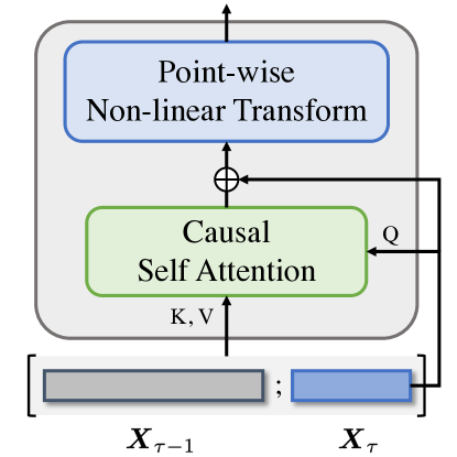
Figure 2: The architecture of Transformer-XL augmenting with a recurrence memory.

2.2 Recurrence Memory Mechanism

To enable the Transformer to consider more contextual information from previous segments, Dai et al. (2019) proposed to augment the Transformer with a recurrence memory which stores the hidden states of previous time steps as extended keys and values, as shown in Figure 2. Concretely, let us consider a memory length of $M$ and memory representations $\boldsymbol{X}_{\tau-1}=[\boldsymbol{x}_{\tau-M+1},\cdots,\boldsymbol{x}_{\tau}]\in\mathbb{R}^{M\times d}$. The extended key and value matrices are obtained by prepend $\boldsymbol{X}_{\tau-1}$ to $\boldsymbol{X}_{\tau}$ before projection:

$$\tilde{\boldsymbol{X}}^{\text{sg}}_{\tau} =[\text{sg}(\boldsymbol{X}_{\tau-1})\circ\boldsymbol{X}_{\tau}]\in\mathbb{R}^{(M+N)\times d},$$ (5)

where $\text{sg}(\cdot)$ stands for stop-gradient which disables gradient propagation to previous segments, and $[\cdot\circ{\cdot}]$ indicates concatenation of hidden states along the length dimension. Extended by the recurrence memory, each query vector can consider contexts even beyond the total context length of the attention $M+N$. As illustrated by Dai et al. (2019), the effective context length grows linearly to the number of layers and the attention context length due to layer-wise reusing.

Another technique necessary to the recurrence memory is the relative positional encodings. By considering only the relative distance between two tokens when computing the attention score, it avoids temporal confusion caused by indexing the same position across segments and injects useful relative bias. Transformer-XL uses the fixed sinusoidal encoding matrix (Vaswani et al., 2017) to provide relative distance bias and learns global bias terms shared across different layers, which can extrapolate to longer contexts with a great reduction of parameters compared to Shaw et al. (2018):

$$\boldsymbol{A}^{{xl}}_{i,j} =\boldsymbol{X}_{i}^{\top}\boldsymbol{W}_{q}^{\top}\boldsymbol{W}_{k}^{E}\boldsymbol{X}_{j}+\boldsymbol{X}_{i}^{\top}\boldsymbol{W}_{q}^{\top}\boldsymbol{W}_{k}^{R}\boldsymbol{R}_{i-j}$$

$$+\boldsymbol{u}^{\top}\boldsymbol{W}_{k}^{E}\boldsymbol{X}_{j}+\boldsymbol{v}^{\top}\boldsymbol{W}_{k}^{R}\boldsymbol{R}_{i-j},$$ (6)

where $\boldsymbol{R}$ is the sinusoid encoding matrix, $\boldsymbol{u},\boldsymbol{v}$ are learnable weight vectors governing the global content and position bias, and $\boldsymbol{W}_{k}^{E},\boldsymbol{W}_{k}^{R}$ are separate key projection matrices for the content and position respectively.

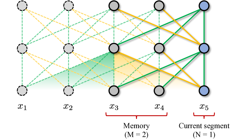
Figure 3: Illustration of LaMemo with a memory length $M=2$ and a target sequence length $N=1$ for clarity. Solid lines stand for the attention connections computed at this iteration while dashed lines represent the previously computed attention.

3 Method

In this section, we describe our method in detail with our motivation to learn better representations for the memory.

3.1 Look-Ahead Attention

Human language is sequential with one word following another, but humans process information usually in a non-sequential way and re-contextualize certain contents for several times. For example, when countering complicated contents during reading, humans usually first store them temporarily in the memory and continue to scan for relevant information if any, and revisit those old contents to refresh their meaning quite often. This dynamic memory refreshing mechanism enables us to thoroughly understand the passage under current contexts.

Existing recurrence memory however, lacks this dynamic contextualization ability. As the representations in the recurrence memory are previously computed conditioned on their past, they are not aware of the current contexts which provide more relevant information for the current token prediction.

To address this limitation, we propose a look-ahead attention that allow the memory to attend to the contexts on their right. Formally, we reuse the notation $\boldsymbol{X}_{\tau}=[\boldsymbol{x}_{\tau+1},\cdots,\boldsymbol{x}_{\tau+N}]\in\mathbb{R}^{N\times d}$ for the representations of the current target sequence and $\boldsymbol{X}_{\tau-1}=[\boldsymbol{x}_{\tau-M+1},\cdots,\boldsymbol{x}_{\tau}]\in\mathbb{R}^{M\times d}$ for the representations of the memory.

Let us consider the $i$-th position of the memory $\boldsymbol{X}_{\tau-1}$, $\boldsymbol{x}_{i}$ can attend to position $\boldsymbol{x}_{j}$ on its right ($j>i$) without causing information leakage as long as $j\leq\tau+1$. Though appealing, this naïve approach requires to calculate an $M$ by $M$ attention map, which would become inefficient and redundant when $M$ is significantly greater than $N$. Actually, since the target segment moves forward $N$ positions at each iteration, we devise an incremental manner of look-ahead attention computation that only requires the newest $N$ positions on the right as key-value pairs.

$$\tilde{\boldsymbol{X}}_{\tau-1}=[{\boldsymbol{x}}_{\tau-N+2},\cdots,{\boldsymbol{x}}_{\tau+1}]\in\mathbb{R}^{N\times d}.$$ (7)

Then the look-ahead attention results computed previously can be effectively reused and interpolated with the current ones (§3.2). Concretely, we formalize the look-ahead attention as follows:

$$\tilde{\boldsymbol{K}}_{\tau-1} =\tilde{\boldsymbol{X}}_{\tau-1}\boldsymbol{W}_{k},\tilde{\boldsymbol{V}}_{\tau-1}=\tilde{\boldsymbol{X}}_{\tau-1}\boldsymbol{W}_{v},$$ (8)

$$\boldsymbol{C}^{\leftarrow}_{\tau-1} =\text{LookAhead-Attn}(\boldsymbol{Q}_{\tau-1},\tilde{\boldsymbol{K}}_{\tau-1},\tilde{\boldsymbol{V}}_{\tau-1})$$

$$=\text{softmax}_{\mbox{ \begin{picture}(5.0,7.0)\polyline(5,0)(5,5)(0,5)(5,0)\end{picture} }}\Big{(}\frac{\boldsymbol{Q}_{\tau-1}\tilde{\boldsymbol{K}}_{\tau-1}^{\top}}{\sqrt{d}}\Big{)}\tilde{\boldsymbol{V}}_{\tau-1},$$ (9)

where $\text{softmax}_{\mbox{ \begin{picture}(5.0,7.0)\polyline(5,0)(5,5)(0,5)(5,0)\end{picture} }}(\cdot)$ masks position $j\leq i$ for the $i$-th row of the input matrix with $-\infty$ before softmax. $\boldsymbol{Q}_{\tau-1}$ is obtained by Eq. (1), and the projection matrices of query, key and value are all shared with the causal attention. We illustrate this in Figure 3 where the look-ahead attention (yello paths) increases the attention window of each memory state to $M$ tokens on its right.

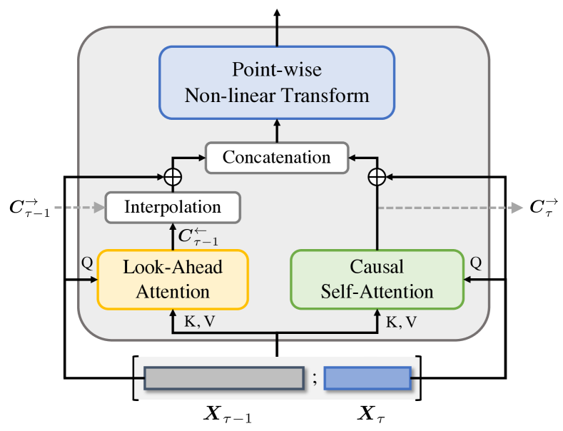
Figure 4: The architecture of LaMemo with look-ahead attention and memory interpolation that refresh the memory dynamically with both the current contexts and the long-term history.

3.2 Memory Interpolation

To save computations for looking-ahead and effectively reuse the attention results of the past, we propose memory interpolation that smoothly interpolates attention results from both the future and the past to provide bi-directional contextualization.

Recall that in the previous iteration, we have calculated the causal context representations $\boldsymbol{C}^{\rightarrow}_{\tau-1}$ of $\boldsymbol{X}_{\tau-1}$ using Eq. 2.1, where each row is a linear combination of the weighted token representations of the previous tokens. In Sec. 3.1, we describe the look-ahead attention which enables $\boldsymbol{X}_{\tau-1}$ to attend to the contexts on their right and computes $\boldsymbol{C}^{\leftarrow}_{\tau-1}$ using Eq. 3.1. Here, we formulate the memory interpolation as the interpolation between the old representations $\boldsymbol{C}^{\rightarrow}_{\tau-1}$ and the new ones $\boldsymbol{C}^{\leftarrow}_{\tau-1}$ with a coefficient vector $\boldsymbol{\alpha}_{\tau-1}\in\mathbb{R}^{M}$ controlling the memorization of the past activations:

$$\boldsymbol{C}^{\leftrightarrow}_{\tau-1} =\text{Mem-Interp}(\boldsymbol{C}^{\rightarrow}_{\tau-1},\boldsymbol{C}^{\leftarrow}_{\tau-1},\boldsymbol{\alpha}_{\tau-1})$$

$$=\boldsymbol{\alpha}_{\tau-1}\text{sg}(\boldsymbol{C}^{\rightarrow}_{\tau-1})+(1-\boldsymbol{\alpha}_{\tau-1})\boldsymbol{C}^{\leftarrow}_{\tau-1}.$$ (10)

The resulted $\boldsymbol{C}^{\leftrightarrow}_{\tau-1}$ which attend to contexts from both directions, are further fed to the non-linear transformation defined in Eq. 3 to update representations in higher layers.

For $\boldsymbol{\alpha}_{\tau-1}$, we define it to be the sum of the normalized attention weights on the previous tokens when calculating $\boldsymbol{C}^{\rightarrow}_{\tau-1}$ (Eq. 2.1):

$$\boldsymbol{\alpha}_{\tau-1}=\frac{\text{sg}(\boldsymbol{s}^{\rightarrow}_{\tau-1})}{\text{sg}(\boldsymbol{s}^{\rightarrow}_{\tau-1})+\boldsymbol{s}^{\leftarrow}_{\tau-1}+\varepsilon},$$ (11)

where $\boldsymbol{s}^{\rightarrow}_{\tau-1}$ is the sum of the unnormalized attention score of $\boldsymbol{C}^{\rightarrow}_{\tau-1}$, which is the denominator of the softmax in Eq. 2.1. Similarly, $\boldsymbol{s}^{\leftarrow}_{\tau-1}$ is the denominator of the softmax in Eq. 3.1. $\varepsilon$ is a small value to prevent zero division error in practice. Then Eq. 3.2 can be derived into a form that resembles the bi-directional attention with the queries attending to positions on both sides (Appendix A). Figure 4 shows the architecture of LaMemo.

Note that the difference between the hidden state reuse in the recurrence memory and our memory interpolation is that they simply reuse the static representations to extend the contexts for attention while we update the memory representations by aggregating weighted attention sum of the history without the need to recompute them.

3.3 Disentangled Relative Positional Encodings

As the look-ahead attention allows the memory to attend to future tokens on its right, we need a relative positional encoding scheme that can generalize to this setting. We start by considering the relative positional encoding in Transformer-XL, as described by Eq. 2.2. When the $i$-th query vector attending to a position $j=i+\Delta>i$, we have $\boldsymbol{R}_{i-j}=\boldsymbol{R}_{-\Delta}$. As defined by Vaswani et al. (2017), $\boldsymbol{R}_{\Delta}\in\mathbb{R}^{D}$ is composed of sine and cosine functions with different frequencies. Since the sine function is odd, $\sin(-\omega\Delta)=-\sin(\omega\Delta)$, we have $\boldsymbol{R}_{-\Delta}\neq\boldsymbol{R}_{\Delta}$ so that it can represent attention in different directions ($\pm$ sign of $\Delta$) with the same relative distance (absolute value of $\Delta$).

However, this approach solely relies on the fixed sinusoid encodings to represent the relative distance and the attention direction. We argue that disentangling them is more effective in capturing these two types of temporal biases and also mitigates the numerical unstability issue. Specifically, we propose to learn two direction-aware global position biases to parameterize the sign and query $\boldsymbol{R}$ with the absolute value of the relative distance:

$$\boldsymbol{A}^{{dis}}_{i,j} =\boldsymbol{X}_{i}^{\top}\boldsymbol{W}_{q}^{\top}\boldsymbol{W}_{k}^{E}\boldsymbol{X}_{j}+\boldsymbol{X}_{i}^{\top}\boldsymbol{W}_{q}^{\top}\boldsymbol{W}_{k}^{R}\boldsymbol{R}_{|i-j|}$$

$$+\boldsymbol{u}^{\top}\boldsymbol{W}_{k}^{E}\boldsymbol{X}_{j}+\boldsymbol{v}_{i-j}^{\top}\boldsymbol{W}_{k}^{R}\boldsymbol{R}_{|i-j|},$$ (12)

where $\boldsymbol{v}_{i-j}=\boldsymbol{v}_{+}$ if $i\geq j$ else $\boldsymbol{v}_{-}$. The global positional bias now explicitly separates the contributions of $\text{sgn}(i-j)$ and $|i-j|$, which can better generalize to long distance in both forward and backward directions.

To illustrate the numerical unstability caused by adapting Eq. 2.2 to $j>i$, we derive the variance of the dot product $\boldsymbol{x}^{T}\boldsymbol{R}_{i-j}$ where $\boldsymbol{x}$ is a random vector. We show that the variance undergoes an oscillation and cannot be properly bounded everywhere when $i$ shifts from $i\geq j$ to $i<j$. Detailed analysis are presented in Appendix B.

4 Experiments

We evaluate LaMemo on both word-level and character-level language modeling tasks and compare with existing Transformer baselines augmented with different types of memory.

4.1 Datasets and Metrics

For word-level language modeling task, we consider Wikitext-103 (Merity et al., 2017), which is the most widely used word-level language modeling benchmark. It contains 103 million tokens for training from 28 thousand wikipedia articles, with an average length of 3.6 thousand tokens per article and a vocabulary size around 260K. We report perplexity (ppl) on the dev and test set.

We also evaluate on two character-level language modeling benchmarks enwik8 and text8 (Mahoney, 2011). Both datasets contain 100 million Wikipedia characters. While enwik8 is unprocessed, text8 is preprocessed by case lowering and filtering to include only 26 letters from a to z and space. On both datasets, we report bit per character (bpc) on the dev and test set.

4.2 Baselines

To directly compare with different types of memory, we consider Transformer-XL and its variations with the same model architecture but different memory mechanism.

Transformer+RPE is the vanilla Transformer (Vaswani et al., 2017) that uses relative positional encodings from Dai et al. (2019) but does not extend the context with additional memory.

Transformer-XL (Dai et al., 2019) is a Transformer model equipped with relative positional encodings and a recurrence memory comprised of hidden states computed in previous time steps to extend the context length of the attention.

Compressive Transformer (Rae et al., 2020) extends Transformer-XL with an external compressive memory that stores compressed hidden states at the temporal level using convolutional networks.

$\infty$-former (Martins et al., 2021) uses continuous space attention to attend over the external memory which consists of continuous signals. They also updated the external memory with recent hidden states to enable unbounded memory capacity.

4.3 Implementation Details

Model	#Params	Mem size	Ext mem size	#FLOPS	dev ppl	test ppl
Transformer+RPE	151M	0	0	148M	28.11	29.14
Transformer-XL (Dai et al., 2019)	151M	150	0	157M	23.42	24.56
Compressive Transformer (Rae et al., 2020)	161M	150	150	169M	-	24.41
$\infty$-former (Martins et al., 2021)	160M	150	150	235M	-	24.22
LaMemo	151M	150	0	191M	22.98	23.77

Table 1: Word-level language modeling results on Wikitext-103. We report ppl (perplexity) on dev and test set. We also report the number of parameters, memory size, external memory size, and the number of FLOPS (floating-point operations) for computing one step prediction on average.

We follow the standard architecture of the Transformer-XL (Dai et al., 2019) that has different configurations for different tasks. Specifically, on Wikitext-103, we use a 16-layer Transformer with 10 attention heads and head dimension 41 equipped with adaptive embeddings (Baevski and Auli, 2019). We control the target sequence length to be 150 and the memory length 150 for all models following the setting of Dai et al. (2019). For the Compressive Transformer and $\infty$-former, we additionally use an external memory of size 150 following the setting of Martins et al. (2021). On the text8 and enwik8 datasets, we use a 12-layer Transformer with 8 heads and head dimension 64. The length of the target sequence and the recurrence memory are both set to 512. In the main results we use the identical evaluation setting to the training phase on all datasets and do not use a longer memory. We use the Pytorch framework (Paszke et al., 2019) and Apex for mixed-precision training. In practice, we found that calculating the exponentials (§3.2) may lead to numerical overflow in mixed-precision mode, so we compute the logarithm of the exponential sum using logsumexp and logaddexp operator. Further details of the dataset and the hyperparameter settings are described in the Appendix C.

4.4 Main Results

Model	dev bpc	test bpc
Dataset: text8
Transformer+RPE	1.232	1.303
Transformer-XL (Dai et al., 2019)	1.172	1.239
LaMemo	1.128	1.196
Dataset: enwik8
Transformer+RPE	1.253	1.240
Transformer-XL (Dai et al., 2019)	1.150	1.128
LaMemo	1.129	1.107

Table 2: Character-level language modeling results on text8 and enwik8. We report bpc (bits-per-character) on the dev and test set.

We show the results of word-level language modeling benchmark Wikitext-103 in Table 1. We first observe that all the models extended with memories significantly outperforms Transformer+RPE. Under the same memory length, LaMemo outperforms Transformer-XL with a clear margin, which demonstrates the effectiveness of learning dynamic memory representations over static ones. When compared to the compressive memory and the unbounded memory that take longer contexts into account, LaMemo still achieves lower perplexity. This indicates that the look-ahead memory allows the language model to exploit the recent contexts to gain performance, while simply increasing the context length yields marginal improvement. This is in accordance with previous findings of how language models utilize contexts (Khandelwal et al., 2018; Sun et al., 2021). In terms of the parameters, LaMemo has the same number of parameters as the Transformer-XL while other baselines use additional parameters in CNN to compress or smooth the hidden states. Lastly, we show the number of FLOPS necessary for computing one step prediction. $\infty$-former has the highest number of FLOPS for resampling enough points from the continuous signal to update the memory using smoothing techniques. LaMemo also incurs additional computations to re-contextualize the memory under the current context. Note that although the Compressive Transformer has lower number of FLOPS than LaMemo, it has an external memory that consumes more GPU memory.

We also present the results of character-level language modeling on text8 and enwik8 datasets in Table 2. We observe similar trends as the results on the word-level benchmark, where LaMemo outperforms Transformer-XL by 0.04 on text8 and 0.02 on enwik8 with the same context length. Additionally, we observe that all models exhibit overfitting on text8, which might be caused by the extremely small vocabulary size of the dataset.

4.5 Ablation Study

We conduct ablation studies on Wikitext-103 to examine the effects of the proposed techniques, i.e., look-ahead attention, memory interpolation, and disentangled relative positional encodings.

We use the same model achitecture and the same target and memory length as the main results. We first study three configurations, including (1) using the Full model setting, (2) ablating the memory interpolation module (w/o mem interp), i.e., set the memorizing coeffecient $\boldsymbol{\alpha}_{\tau-1}=0$, and (3) ablating the look-ahead attention (w/o look-ahead), i.e., only use the causal context representations $\boldsymbol{C}^{\rightarrow}_{\tau-1}$ in each layer. As shown in the First three rows in Table 3, both the memory interpolation and the look-ahead attention are indispensible for achieving the best performance. Additionaly, we found that cancelling out memory interpolation leads to a worse performance, which indicates that the distant past still provides additional information beyond the current context.

Configuration	Encoding	dev ppl	test ppl
Full	Ours	22.98	23.77
w/o mem interp	Ours	23.67	24.90
w/o look-ahead	Ours	23.42	24.56
Full	Dai et al. (2019)	FAIL	FAIL

Table 3: Ablation study on Wikitext-103. We investigate three model configurations and two encoding schemes.

The second study targets at studying different encoding schemes. We substitute our encodings with the RPE of Transformer-XL Dai et al. (2019) and run multiple experiments with 3 different random seeds, but all the models fail to converge. We plot the training curves using two encodings in Figure 8 in Appendix B, where we observe that our disentangled RPE is more stable during training and achieves lower perplexity.

5 Extrapolating to Longer Contexts

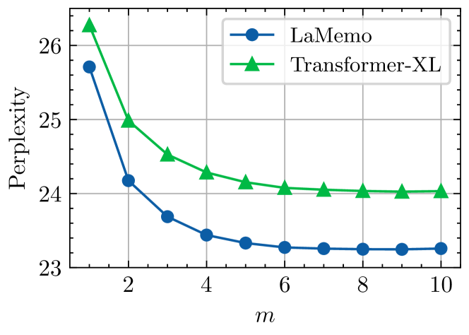
Figure 5: Test perplexity of LaMemo and Transformer-XL when extrapolating to longer contexts during inference, where $m$ is the ratio of the memory length to the target length.

In this section, we extrapolate the models to longer contexts during inference to study the effect of dynamic contextualization to the distant past.

We fix the length of the target sequence to $64$ and extrapolate the trained models to longer memory length $64\times m$ during inference, where $m=1,\cdots,10$. We compare the perplexity of LaMemo and Transformer-XL trained on Wikitext-103 when augmented by a memory with different length. As shown in Figure 5, LaMemo consistently achieves lower perplexity than Transformer-XL when extraploating to longer contexts, while the performance of both models saturate when $m$ is over 7. Additionally, we observe that the gap of perplexity between the two models increases when taking longer contexts into account. This demonstrates the effectiveness of dynamically refreshing the distant memory representations under the current context.

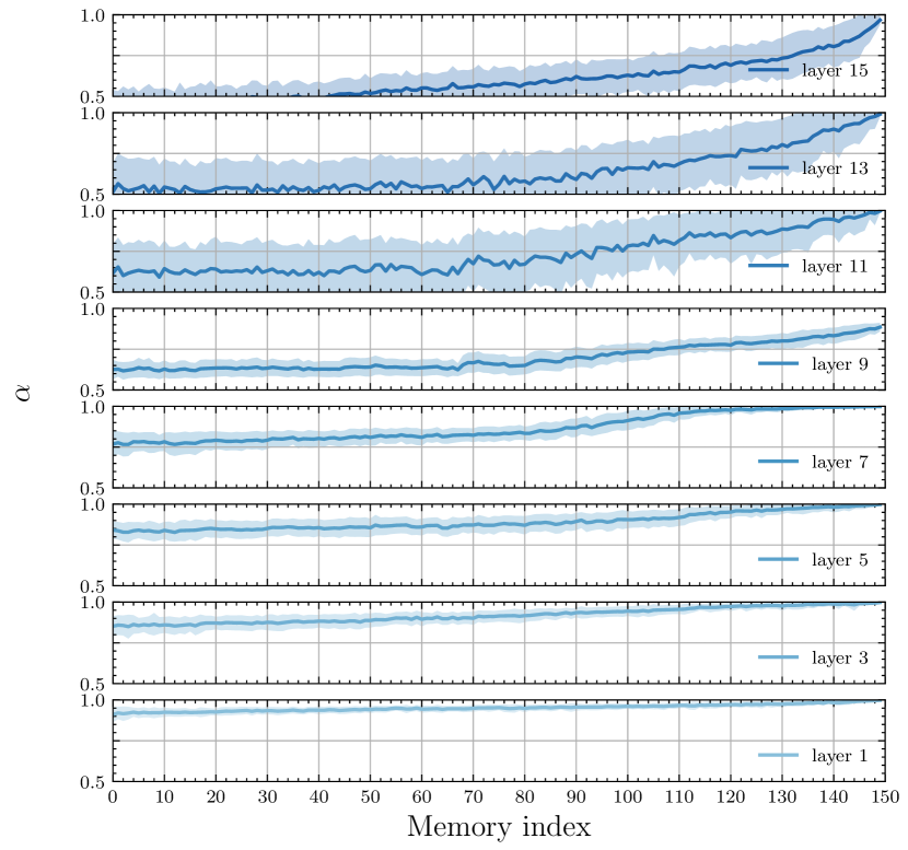
Figure 6: The memorizing coefficient $\alpha$ of different layers in a 16-layer model with a same memory and target length of 150. Smaller index means older memory.

6 Attention Analysis

In this section, we analyze the attention distribution of LaMemo to validate the effectiveness of utilizing bi-directional contexts with look-ahead attention.

We first visualize the memorizing coefficient $\alpha$ which stands for the portion of the past activations in the current memory representations. As show in Figure 6, we plot $\alpha$ in different layers as a function of the memory index averaged on 100 text segments. We observe that in lower layers the memory mainly attends to the past ($\alpha\approx 1.0$). We conjecture that long-term bi-directionality is not necessary for low-level representations such as lexical features. In higher layers, the memory substantially utilizes the future contents to refresh the high-level representations, especially for the old memory state with a small memory index.

Next, we visualize the attention weight distribution on the context tokens when predicting each target token in Figure 1. For every token, we take the maximal attention weight in each interval of 5 tokens on its left and scale to a context length of 100. The result indicates that LaMemo learns better memory represetations by attending to the right-side tokens, which increases the memory utilization when predicting the target token.

7 Case Study

We present the generated texts of LaMemo and Transformer-XL trained on Wikitext-103 in Appendix D. Both models maintain a memory size of 512, and we seed them with the same context randomly sampled from the test set and generate 256 tokens using top-p sampling (Holtzman et al., 2020) with $p=0.95$.

8 Related Work

The Transformer (Vaswani et al., 2017), with its pair-wise modeling ability of the input, becomes prevailing for sequence modeling, especially long sequence processing tasks, such as long text generation (Tan et al., 2021; Ji and Huang, 2021), long document QA (Beltagy et al., 2020; Ainslie et al., 2020), language modeling (Dai et al., 2019; Rae et al., 2020), video processing (Wu et al., 2019), and etc. Specifically, language modeling (Merity et al., 2017) which requires processing documents with thousands of tokens has become a natural testbed for benchmarking this long-term processing ability. However, due to the quadratic time and space complexity of self-attention, scaling to inputs with thousands of tokens is computationally prohibitive.

One line of work investigated the linear-time attention mechanism to mitigate the scability issue of Transformer. Linformer (Wang et al., 2020) projects the inputs to lower dimension in length and approximates the full attention with a low-rank factorization. Linear Transformer (Katharopoulos et al., 2020) regards the self-attention as a kernel function and uses a linear dot-product as a substitute. Choromanski et al. (2021) and Peng et al. (2021) proposed to approximate the softmax more precisely with the expectation of the dot-product of random features. Although achieving substantial improvements on benchmarks designated for long inputs (Tay et al., 2021). These methods, however, focus on approximating the full attention with low-rank factorizations or kernel functions, which compromise the expressiveness and robustness of the original softmax attention, are reported to be inferior to the simple local attentions on real world language processing tasks (Xiong et al., 2021).

Our work falls in another line, which augments the Transformer with a parametrized memory to store critical history information. Memory-augmented networks (Graves et al., 2014; Weston et al., 2015; Sukhbaatar et al., 2015) have been studied in the context of recurrent neural networks for a long time, but are mostly restricted to small and synthetic datasets. With the rapid development of Transformer, various works start to adapt memories to this architecture.

Dai et al. (2019) first extended Transformer with a recurrence memory that caches hidden states computed in previous steps for the target tokens to attend to. Rae et al. (2020) further extended the context with an external memory that stores compressed hidden states at the temporal level. Martins et al. (2021) used continuous space attention to attend over the old history and updated the memory with recent hidden states to enable unbounded memory capacity. Wu et al. (2021) proposed to use the encoder-decoder architecture to encode the memory states with previous text segments and pass this memory to future time steps. Instead of using a fixed-size attention span for different layers, Sukhbaatar et al. (2019) and Correia et al. (2019) proposed to learn dynamic attention spans for different attention heads, which greatly reduced the computations. These works focused on enabling the Transformer to access contents in long distance, but did not consider to learn better memory representations by refreshing the old memory under the current context. Our work is orthogonal to learning adaptive attention spans and can be combined with this technique to reduce the complexity.

9 Conclusion

We present LaMemo, a memory mechanism that allows the memory states to incrementally attend to the right-side tokens and interpolates with the old memory states on the left side, which enables the memory to interact with bi-directional contexts with a complexity linear in memory length. Experiments on three language modeling datasets demonstrate the superiority of LaMemo over baselines with various types of memory mechanisms. We also found that LaMemo increases the utilization of older memory states when predicting the target tokens, and yields a higher performance boost when extrapolating to longer memory length, which indicates the effectiveness of recontextualizing the memory under the current context.

Appendix A Derivation of Memory Interpolation

We derive Eq. 3.2 into the form of standard self-attention in the following:

$$\boldsymbol{C}^{\leftrightarrow}_{\tau-1} =\boldsymbol{\alpha}_{\tau-1}\text{sg}(\boldsymbol{C}_{\tau-1}^{\rightarrow})+(1-\boldsymbol{\alpha}_{\tau-1})\boldsymbol{C}_{\tau-1}^{\leftarrow}.$$

We consider the $i$-th row of $\boldsymbol{C}^{\leftrightarrow}_{\tau-1}$, denoted as $\boldsymbol{c}_{i}^{\leftrightarrow}$. We omit the stop-grad operation $\textrm{sg}(\cdot)$ and substitute $\alpha$ with the result from Eq. 11:

$$\boldsymbol{c}_{i}^{\leftrightarrow} =\alpha_{i}\boldsymbol{c}_{i}^{\rightarrow}+(1-\alpha_{i})\boldsymbol{c}_{i}^{\leftarrow}$$

$$=\frac{s_{i}^{\rightarrow}}{s_{i}^{\rightarrow}+s_{i}^{\leftarrow}}\boldsymbol{c}_{i}^{\rightarrow}+\frac{s_{i}^{\leftarrow}}{s_{i}^{\rightarrow}+s_{i}^{\leftarrow}}\boldsymbol{c}_{i}^{\leftarrow},$$

where $s_{i}^{\rightarrow}$, $s_{i}^{\leftarrow}$ is the denominator of the softmax when computing $\boldsymbol{c}_{i}^{\rightarrow}$, $\boldsymbol{c}_{i}^{\leftarrow}$ respectively:

$$s_{i}^{\rightarrow} =\sum_{j\leq i}\exp\Big{(}\frac{\boldsymbol{q^{\prime}}_{i}^{\top}\boldsymbol{k^{\prime}}_{j}}{\sqrt{d}}\Big{)}=\sum_{j\leq i}\text{sim}(\boldsymbol{q^{\prime}}_{i},\boldsymbol{k^{\prime}}_{j}),$$

$$s_{i}^{\leftarrow} =\sum_{j>i}\exp\Big{(}\frac{\boldsymbol{q}_{i}^{\top}\boldsymbol{k}_{j}}{\sqrt{d}}\Big{)}=\sum_{j>i}\text{sim}(\boldsymbol{q}_{i},\boldsymbol{k}_{j}),$$

where $(\boldsymbol{q}^{\prime}_{i},\boldsymbol{k}^{\prime}_{j})$ and $(\boldsymbol{q}_{i},\boldsymbol{k}_{j})$ are two sets of query-key vectors computed in the previous and this text segment respectively for the same position pair $(i,j)$ . Then we have:

$$\boldsymbol{c}_{i}^{\leftrightarrow}=\frac{\sum_{j\leq i}\text{sim}(\boldsymbol{q^{\prime}}_{i},\boldsymbol{k^{\prime}}_{j})}{\sum_{j\leq i}\text{sim}(\boldsymbol{q^{\prime}}_{i},\boldsymbol{k^{\prime}}_{j})+\sum_{j>i}\text{sim}(\boldsymbol{q}_{i},\boldsymbol{k}_{j})}\boldsymbol{c}_{i}^{\rightarrow}$$

$$+\frac{\sum_{j>i}\text{sim}(\boldsymbol{q}_{i},\boldsymbol{k}_{j})}{\sum_{j\leq i}\text{sim}(\boldsymbol{q^{\prime}}_{i},\boldsymbol{k^{\prime}}_{j})+\sum_{j>i}\text{sim}(\boldsymbol{q}_{i},\boldsymbol{k}_{j})}\boldsymbol{c}_{i}^{\leftarrow}$$

$$=\frac{\sum_{j\leq i}\text{sim}(\boldsymbol{q^{\prime}}_{i},\boldsymbol{k^{\prime}}_{j})\boldsymbol{v^{\prime}}_{j}+\sum_{j>i}\text{sim}(\boldsymbol{q}_{i},\boldsymbol{k}_{j})\boldsymbol{v}_{j}}{\sum_{j\leq i}\text{sim}(\boldsymbol{q^{\prime}}_{i},\boldsymbol{k^{\prime}}_{j})+\sum_{j>i}\text{sim}(\boldsymbol{q}_{i},\boldsymbol{k}_{j})}$$

$$=\sum_{j}\beta_{j}\boldsymbol{\tilde{v}}_{j},$$

where $\sum_{j}\beta_{j}=1$. Finally, we derive $\boldsymbol{c}_{i}^{\leftrightarrow}$ as the weighted sum of the value vectors $\boldsymbol{\tilde{v}}_{j}$ from both the past ($j\leq i$) and the future ($j>i$) of the position $i$.

Appendix B Unstability Analysis of the RPE in Transformer-XL

We conjecture that the unstability of Eq. 2.2 stems from the terms involving the dot-product of $\boldsymbol{R}_{i-j}$ and another vector. So we start by considering the variance of $\boldsymbol{x}^{\top}\boldsymbol{R}_{i-j}$ where $\boldsymbol{x}\in\mathbb{R}^{d}$ is a random vector. Without loss of generality, we assume that $\boldsymbol{x}$ has zero mean and a variance of $\boldsymbol{\sigma}$:

$$\textrm{E}(x_{k}) =0,\ \forall k\in[1,\cdots,d]$$

$$\textrm{Var}(x_{k}) =\sigma_{k,k},\ \forall k\in[1,\cdots,d]$$

$$\textrm{Cov}(x_{k},x_{l}) =\sigma_{k,l},\ \forall l\neq k\in[1,\cdots,d]$$

Let $i-j=\Delta$. According to Vaswani et al. (2017), $\boldsymbol{R}_{\Delta}$ takes the following form:

$$\boldsymbol{R}_{\Delta}= [\sin(\omega_{1}\Delta),\cos(\omega_{1}\Delta),$$

$$\cdots,\sin(\omega_{d/2}\Delta),\cos(\omega_{d/2}\Delta)],$$

where $w_{k}=10000^{-2k/d}$. Then the dot-product $\boldsymbol{x}^{\top}\boldsymbol{R}_{\Delta}$ can be derived into the linear combination of sine and cosine functions:

$$\boldsymbol{x}^{\top}\boldsymbol{R}_{\Delta} =\sum_{k=1}^{d/2}x_{2k-1}\sin(\omega_{k}\Delta)+x_{2k}\cos(\omega_{k}\Delta),$$

where we can easily derive that $\textrm{E}(\boldsymbol{x}^{\top}\boldsymbol{R}_{\Delta})=0$. According to the variance-expectation formula: $\textrm{Var}(x)=\textrm{E}[x^{2}]-\textrm{E}[x]^{2}$, we can simplify the variance $\textrm{Var}(\boldsymbol{x}^{\top}\boldsymbol{R}_{\Delta})$ in the following:

$$\textrm{Var}(\boldsymbol{x}^{\top}\boldsymbol{R}_{\Delta})$$

$$=\textrm{E}\Big{[}\big{(}\sum_{k=1}^{d/2}x_{2k-1}\sin(\omega_{k}\Delta)+x_{2k}\cos(\omega_{k}\Delta)\big{)}^{2}\Big{]}$$

$$=\sum_{k=1}^{d/2}\textrm{E}[x^{2}_{2k-1}]\sin^{2}(\omega_{k}\Delta)+\textrm{E}[x^{2}_{2k}]\cos^{2}(\omega_{k}\Delta)$$

$$+2\sum_{k=1}^{d/2}\sum_{l=1,l\neq k}^{d/2}\textrm{E}[x_{2k-1}x_{2l}]\sin(\omega_{k}\Delta)\cos(\omega_{l}\Delta).$$

We further simplify the above equation by assuming that all the elements have the same variance $\sigma_{s}$, and all pairs of distinct elements have the same covariance $\sigma_{c}$:

$$\textrm{Var}(\boldsymbol{x}^{\top}\boldsymbol{R}_{\Delta})=\sum_{k=1}^{d/2}\sigma_{s}[\sin^{2}(\omega_{k}\Delta)+\cos^{2}(\omega_{k}\Delta)]$$

$$+2\sum_{k=1}^{d/2}\sum_{l=1,l\neq k}^{d/2}\sigma_{c}\sin(\omega_{k}\Delta)\cos(\omega_{l}\Delta)$$

$$=\frac{d}{2}\sigma_{s}+2\sigma_{c}g(\Delta),$$

where $g(x)=\sum_{k=1}^{d/2}\sum_{l=1,l\neq k}^{d/2}\sin(\omega_{k}x)\cos(\omega_{l}x)$ is an odd function.

We consider the value of $g(x)$ when $x\approx 0$. Since $\sin(\omega_{k}x)\approx\omega_{k}x$, $\cos(\omega_{k}x)\approx 1$, we have:

$$g(x) \approx\sum_{k=1}^{d/2}\sum_{l=1}^{d/2}\omega_{k}x$$

$$=\frac{d}{2}\sum_{k=1}^{d/2}w_{k}x$$

$$=\frac{xd}{2}\sum_{k=1}^{d/2}\Big{(}\frac{1}{10000^{2/d}}\Big{)}^{k}$$

$$\approx\frac{d}{2((10^{8})^{1/d}-1)}\cdot x=\gamma_{d}\cdot x.$$

Since $a^{x}\approx 1+x\ln a$ when $x\approx 0$, we derive that $\gamma_{d}\approx\frac{d^{2}}{2\ln 10^{8}}$ with the grow of $d$. This causes $g(x)$ to have a very steep slope near 0. Since $g(x)$ is an odd function, the value of $g(\Delta)$ and $g(-\Delta)$ will have a huge gap ($\Delta$ is a small positive value). To validate this, we plot the function of $g(x)$ when $d=64$ in Figure 7.

Overall, the variance of $\boldsymbol{x}^{\top}\boldsymbol{R}_{\Delta}$ is composed of two terms, the first being $\sigma_{s}$ multiplied by a constant factor $d/2$, and the second being $\sigma_{c}$ multiplied by $g(\Delta)$. Note that $\sigma_{s}$ is strictly positive, while $\sigma_{c}$ does not have this restriction. Due the asymptotic behavior of $g(\Delta)$ near 0, i.e., $\mathcal{O}(d^{2}\Delta)$, we cannot find a proper $\sigma_{c}$ that makes $\textrm{Var}(\boldsymbol{x}^{\top}\boldsymbol{R}_{\Delta})$ bounded by $\mathcal{O}(d\sigma_{s})$ for every $\Delta$ that takes its value from both the positive and negative integers.

Finally, we plot the training curves of the two models using the RPE in Transformer-XL (xl-rpe) and our disentangled RPE (dis-rpe) in Figure 8 where we observed that the xl-rpe suffers from numerical unstability during training.

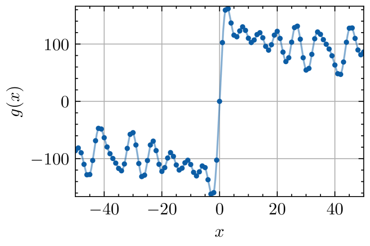
Figure 7: The plot of $g(x)$ when $d=64$. We see that $g(x)$ is symmetric with respect to the origin. The value of $g(x)$ when $x$ approaches zero from the left and right diverge greatly.

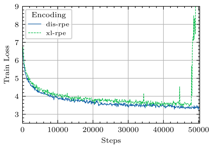
Figure 8: Comparison of the training dynamics using different encoding schemes: the disentangled RPE (dis-rpe) and the RPE of Transformer-XL (xl-rpe).

Appendix C Experimental Details

C.1 Dataset Details

Wikitext-103 dataset is extracted from the set of verified Good and Featured articles on English Wikipedia. The dataset retains the original case, punctuation and numbers, and covers a broad range of domains, e.g., science, culture, bibliography, and etc. The dataset is available under the Creative Commons Attribution-ShareAlike (CC BY-SA) License.

enwik8 dataset is the test set data of the Large Text Compression Benchmark which contains the first 100 million bytes of English Wikipedia dump on Mar. 3, 2006. All characters are encoded in UTF-8. This dataset is licensed under the CC BY-SA License.

text8 dataset contains the first 100 million bytes of the clean text of Wikipedia that retains only regular articles and image captions. All the letters are converted into lower case, and only letters in the 27 character alphabet, namely letters a-z and nonconsecutive spaces, are preserved. This dataset is licensed under the CC BY-SA License.

The statistics of the three datasets is shown in Table 4.

Dataset	train / dev / test
Wikitext-103	103,227,021 / 217,646 / 245,569
enwik8	88,982,818 / 4,945,742 / 4,943,417
text8	89,999,999 / 4,999,999 / 5,000,000

Table 4: Statistics of the datasets used in the experiments. For Wikitext-103, we use the official split from Merity et al. (2017) and present the number of tokens in each split. For enwik8 and text8, we use the split from Dai et al. (2019) and report the number of characters for each split.

C.2 Model Configurations

We follow the base model configuration of Dai et al. (2019). On Wikitext-103, we use the Transformer model with 16 layers, 10 attention heads with a head dimension of 41. The inner dimension size of the feedforward layer is 2100. We use a dropout rate of 0.1 and no attention dropout. To cope with the large vocabulary, we use the adaptive embeddings (Baevski and Auli, 2019). We set the memory length to 150 and the target sequence length to 150 as well. On text8 and enwik8 datasets, we use the Transformer model with 12 layers, 8 attention heads with a head dimension of 64. The inner dimension size of the feedforward layer is 2048. We use a dropout rate of 0.1 and no attention dropout. We set the memory length to 512 and the target length to 512. Specifically, our LaMemo uses the disentangled relative positional encodings described in Sec. 3.3. The look-ahead attention shares the query, key and value projection matrices with those in the causal attention.

C.3 Training Settings

We trained the models using Adam (Kingma and Ba, 2015) optimizer, with no warmup. We used a learning rate of $2.5\times 10^{-4}$ which decayed to 0 at the end of training with a cosine schedule. On Wikitext-103, we trained the model with 250K steps using a batch size of 64. On enwik8 and text8, we trained the model with 100K steps using a batch size of 40. We conducted our experiments on 2 Tesla V100.

C.4 Hyperparameters

We present the hyperparameter search space in Table 5. The number of hyperparameter search trials was 10. We adopted a manual search to select the hyperparameters, and the selection criterion was ppl/bpc on the dev set. We did not use early stopping during training.

Hyper-parameter	Search Space
Learning Rate	choice[1e-4, 2.5e-4, 5e-4]
Learning Rate Schedule	choise[linear, cosine]
Warmup Steps	choice[0, 1000, 2000]
Maximum Gradient Norm	choice[0.25, 0.5, 1.0]
Epsilon (Sec. 3.2)	choice[1e-6, 1e-5, 1e-4]
Optimizer	Adam
Epsilon (for Adam)	1e-8
Momentum (for Adam)	$\beta_{1}=0.9,\beta_{2}=0.999$

Table 5: Hyperparameter search space. choice indicates that the listed numbers will be chosen with the same probability. Best-found hyperparameters are in boldface.

Appendix D Generated Examples

In this section, we present the examples generated by LaMemo and Transformer-XL trained on the Wikitext-103 dataset. Both models maintain a memory with a length of 512. We randomly select a piece of text from the test set as the context and allow both models to generate 256 tokens following the context. We use top-p sampling with $p=0.95$ and detokenize the context and the generated texts to facilitate reading. We present the exmples in Table 6 and 7. We present our major findings below:

• Both models are able to hallucinate imaginary contents fairly relevant to the limited contexts given as prompts.

• Transformer-XL sometimes generates topic-irrelevant contents without further elaboration (marked by underline), while LaMemo stays on topic more closely during the course of generation.

• Transformer-XL suffers more sever repetition issues (marked in boldface) than LaMemo both lexically and semantically.

Context: = Shackleton ( crater ) = Shackleton is an impact crater that lies at the south pole of the Moon. The peaks along the crater’s rim are exposed to almost continual sunlight, while the interior is perpetually in shadow (a Crater of eternal darkness). The low-temperature interior of this crater functions as a cold trap that may capture and freeze volatiles shed during comet impacts on the Moon. Measurements by the Lunar Prospector spacecraft showed higher than normal amounts of hydrogen within the crater, which may indicate the presence of water ice. The crater is named after Antarctic explorer Ernest Shackleton. = = Description = = The rotational axis of the Moon lies within Shackleton, only a few kilometers from its center. The crater is 21 km in diameter and 4.2 km deep. From the Earth, it is viewed edge-on in a region of rough, cratered terrain. It is located within the South Pole-Aitken basin on a massif. The rim is slightly raised about the surrounding surface and it has an outer rampart that has been only lightly impacted. No significant craters intersect the rim, and it is sloped about 1.5 ° toward the direction 50 – 90 ° from the Earth. The age of the crater is about 3.6 billion years and it has been in the proximity of the south lunar pole for at least the last two billion years. Because the orbit of the Moon is tilted only 5 ° from the ecliptic, the interior of this crater lies in perpetual darkness. Estimates of the area in permanent shadow were obtained from Earth-based radar studies. Peaks along the rim of the crater are almost continually illuminated by sunlight , spending about 80 – 90 % of each lunar orbit exposed to the Sun. Continuously illuminated mountains have been termed peaks of eternal light and have been predicted to exist since the 1900s. The shadowed portion of the crater was imaged with the Terrain Camera of the Japanese SELENE spacecraft using the illumination of sunlight reflected off the rim. The interior of the crater consists of a symmetrical 30 ° slope that leads down to a 6.6 km diameter floor. The handful of craters along the interior span no more than a few

LaMemo Generation: kilometres of plains. A slight rotation is observed in the crater that now bears significant elements like snow, ice, and water ice. In other areas of the crater there are indications that the nature of the alpine ice layer provides some protection to the craters by increasing their brightness. The craters seem to be cut by an ice thickness of 10 cm (4 in). Images show their prominence, varying from a visible plateau to a multi-ring topography, indicating that they are present (a major component) in the craters. Their interior has a considerable surface area of dry ice. As seen from Earth, the initial craters are marked by slow-moving metal-bearing mudstone-covered rock that has a surface of substantial amounts of coal, calcium, lead and sodium alloy, carbon monoxide, nitrogen oxides, and silicon dioxide. All are developed by processes such as heat transfer by the advancing radiation pressure. The least dense feature along the surface of the Moon is the large resurfacing event. There is no view that these rocks remain melting to about 90 °C (150 °F), but that their surface shine is dark and their outer layers are light, reflecting vertical oil. This late flank and early 1970s discovery was announced in 1982, as a substantial amount of ice. A parallel lava

Transformer-XL Generation: kilometres. During the hundreds of years after its formation, the crater now has significant seismic activity in the vicinity. Most craters are dome-shaped and are usually constructed of sedimentary materials that have been deposited during alpine ice times. The upper surface of the crater is covered with higher layers of rock that are cut by an extensive thickness of debris. The debris reaches the top of a mountain and comes in contact with visible ground planes. People are often observed wearing headgear of degrading materials such as clothing and boots, their shoes or hats, or even working on the surface. Below the crater. As the crater faces the crater it has thick, thin pipes or scarps. A total of more than 200 caves have been excavated, down to some 40 m by 20 m. This exceeding the margin of the crater where it actually passes through is considered to be very high. Other geologic features by the advancing magnetic field have been reported from the crater. However, in 1992, scientists announced they would study this area again. The crater was once a common feature of the Post Lunar System. Its medieval boundaries were not fixed in the orbital plane of Mercury. An individual crater had been called “ Discovery crater ” and one referred to as “ Bear crater ”, although it is likely that an additional crater was called

Table 6: Example 1 generated by LaMemo and Transformer-XL given a context prompt from the test set of Wikitext-103. Original Wikipedia page: https://en.wikipedia.org/wiki/Shackleton_(crater).

Context: Nero was not expected to become Emperor because his maternal uncle, Caligula, had begun his reign at the age of 24 with enough time to produce his own heir. Nero ’s mother, Agrippina, lost favour with Caligula and was exiled in 39 after her husband ’s death. Caligula seized Nero ’s inheritance and sent him to be brought up by his less wealthy aunt, Domitia <unk>, who was the mother of Valeria <unk>, Claudius ’s third wife. Caligula, his wife <unk> and their infant daughter Julia Drusilla were murdered on 24 January 41. These events led Claudius, Caligula ’s uncle, to become emperor. Claudius allowed Agrippina to return from exile. Claudius had married twice before marrying Valeria <unk>. His previous marriages produced three children including a son, Drusus, who died at a young age. He had two children with <unk> – Claudia Octavia (born 40) and Britannicus (born 41). <unk> was executed by Claudius in the year 48. In 49 AD , Claudius married a fourth time, to Nero ’s mother Agrippina, despite her being his niece. To aid Claudius politically, young Nero was adopted in 50 and took the name Nero Claudius Caesar Drusus Germanicus (see adoption in Rome). Nero was older than his stepbrother Britannicus, and thus became heir to the throne. Nero was proclaimed an adult in 51 at the age of 14. He was appointed proconsul, entered and first addressed the Senate, made joint public appearances with Claudius, and was featured in coinage. In 53, he married his stepsister Claudia Octavia. = = Emperor (54 – 68 AD) = = = = = Early rule = = = Claudius died in 54 and Nero, taking the name Nero Claudius Caesar Augustus Germanicus, was established as Emperor. Though accounts vary, many ancient historians state Agrippina poisoned Claudius. According to Pliny the Elder, she used poison mushrooms. It is not known how much Nero knew or if he was even involved in the death of Claudius. Suetonius wrote “ … for even if he was not the instigator of the emperor ’s death , he was at least privy to it, as he openly admitted; for he used afterwards to laud mushrooms, the vehicle in which the poison was administered to Claudius, as ‘ the food of the gods , ’ as the Greek proverb has it. At any rate, after Claudius’ death he vented on him every kind of insult, in act and word, charging him now with folly and now with cruelty; for it was a favourite joke of his to say that Claudius had ceased ‘ to play the fool ’ among mortals, lengthening the first syllable of the word <unk>, and he disregarded many of his decrees and acts as the work of a madman and a <unk>. Finally, he neglected to enclose the place where his body was burned except with a low and mean wall. ” According to Suetonius; Nero became Emperor at the age of 17 when the news of Claudius’ death was made known , making him the youngest emperor at that time Although, what Suetonius may have meant is that he was

LaMemo Generation: killed as a result of the subsequent anti-Caligula propaganda. At some time after 47 AD, Nero retired to his villa at Baiae. The combination of a curse that led to the death of Agrippa, and a duel between Claudius and his own son Drusus, may have encouraged the young Emperor to fire his own stela. = = = = = Germanicus = = = = = After becoming emperor, Nero received letters from Suetonius, which finally followed him on 28 May 44 AD with a letter to Claudius, completing the Emperor ’s plot. The letters were printed in Latin. Claudius’ plot was offered to Caligula by Agrippina the Elder, a woman from Kent, but she declined. Further letters from Gaius and Nero are known from the reigns of Tiberius and Caligul , though none of them mention Caligula. Germanicus’ conspiracy had developed into a protracted affair. His wife Antonia, his sister Agrippina ’s sister and grandmother, had refused to accept him because she believed they were connected for communication, but the Via Flavia was left to her husband and Agrippina the Elder, whom she had defeated in her husband ’s palace. Both had been sent through Gibraltar to compete for power. Gaius and Nero were outraged that Agrippina was supposed to be ready to support Caligula; Suetonius says that Nero insisted on making

Transformer-XL Generation: killed as a result of poison and was deemed a good comedian. At now and then he had adopted Nero as his heir. Although Nero ’s rule was as close as he was to his father to his daughter Agrippina, he was not to physically exhibit any ill degree of higher kingship but to deny it. The Augustan History describes him as having been strongly willed, possessing an excellent hand and often claiming the title “ Augustus Caesar ”, and often referred to him as Caesar ’s “ paternal heir ”. The Augustan History, however, asserts that he was no longer in China, and therefore he was raised as a Roman Hercules rather than a Roman citizen. Claudius Claudius was added as a junior emperor in 53 AD; he was crowned emperor in 61 AD. = = = = As Augustus I = = = = Claudius had developed a keen interest in Claudius in divination, a practice which later developed into his incarnation as a youth figure in Julius Caesar. Claudius ’ grandfather, Leo I, ascended the throne in 23 AD and spent time in Rome, as did Claudius, who defeated Claudius in 42 AD. Claudius departed Rome after the death of Agrippa III in 65 AD. During the following years, Claudius was temporarily imprisoned in Rome, although possibly simply regulating the use of the captive dogs

Table 7: Example 2 generated by LaMemo and Transformer-XL given a context prompt from the test set of Wikitext-103. Original Wikipedia page: https://en.wikipedia.org/wiki/Nero.

References

- Ainslie et al. (2020) Joshua Ainslie, Santiago Ontañón, Chris Alberti, Vaclav Cvicek, Zachary Fisher, Philip Pham, Anirudh Ravula, Sumit Sanghai, Qifan Wang, and Li Yang. 2020. ETC: encoding long and structured inputs in transformers. In Proceedings of the 2020 Conference on Empirical Methods in Natural Language Processing, EMNLP 2020, Online, November 16-20, 2020, pages 268–284. Association for Computational Linguistics.
- Ba et al. (2016) Lei Jimmy Ba, Jamie Ryan Kiros, and Geoffrey E. Hinton. 2016. Layer normalization. CoRR, abs/1607.06450.
- Baevski and Auli (2019) Alexei Baevski and Michael Auli. 2019. Adaptive input representations for neural language modeling. In 7th International Conference on Learning Representations, ICLR 2019, New Orleans, LA, USA, May 6-9, 2019. OpenReview.net.
- Bahdanau et al. (2015) Dzmitry Bahdanau, Kyunghyun Cho, and Yoshua Bengio. 2015. Neural machine translation by jointly learning to align and translate. In 3rd International Conference on Learning Representations, ICLR 2015, San Diego, CA, USA, May 7-9, 2015, Conference Track Proceedings.
- Beltagy et al. (2020) Iz Beltagy, Matthew E. Peters, and Arman Cohan. 2020. Longformer: The long-document transformer. CoRR, abs/2004.05150.
- Choromanski et al. (2021) Krzysztof Marcin Choromanski, Valerii Likhosherstov, David Dohan, Xingyou Song, Andreea Gane, Tamás Sarlós, Peter Hawkins, Jared Quincy Davis, Afroz Mohiuddin, Lukasz Kaiser, David Benjamin Belanger, Lucy J. Colwell, and Adrian Weller. 2021. Rethinking attention with performers. In 9th International Conference on Learning Representations, ICLR 2021, Virtual Event, Austria, May 3-7, 2021. OpenReview.net.
- Correia et al. (2019) Gonçalo M. Correia, Vlad Niculae, and André F. T. Martins. 2019. Adaptively sparse transformers. In Proceedings of the 2019 Conference on Empirical Methods in Natural Language Processing and the 9th International Joint Conference on Natural Language Processing, EMNLP-IJCNLP 2019, Hong Kong, China, November 3-7, 2019, pages 2174–2184. Association for Computational Linguistics.
- Dai et al. (2019) Zihang Dai, Zhilin Yang, Yiming Yang, Jaime G. Carbonell, Quoc Viet Le, and Ruslan Salakhutdinov. 2019. Transformer-xl: Attentive language models beyond a fixed-length context. In Proceedings of the 57th Conference of the Association for Computational Linguistics, ACL 2019, Florence, Italy, July 28- August 2, 2019, Volume 1: Long Papers, pages 2978–2988. Association for Computational Linguistics.
- Graves et al. (2014) Alex Graves, Greg Wayne, and Ivo Danihelka. 2014. Neural turing machines. CoRR, abs/1410.5401.
- He et al. (2016) Kaiming He, Xiangyu Zhang, Shaoqing Ren, and Jian Sun. 2016. Deep residual learning for image recognition. In 2016 IEEE Conference on Computer Vision and Pattern Recognition, CVPR 2016, Las Vegas, NV, USA, June 27-30, 2016, pages 770–778. IEEE Computer Society.
- Holtzman et al. (2020) Ari Holtzman, Jan Buys, Li Du, Maxwell Forbes, and Yejin Choi. 2020. The curious case of neural text degeneration. In 8th International Conference on Learning Representations, ICLR 2020, Addis Ababa, Ethiopia, April 26-30, 2020. OpenReview.net.
- Huang et al. (2018) Cheng-Zhi Anna Huang, Ashish Vaswani, Jakob Uszkoreit, Noam Shazeer, Curtis Hawthorne, Andrew M. Dai, Matthew D. Hoffman, and Douglas Eck. 2018. An improved relative self-attention mechanism for transformer with application to music generation. CoRR, abs/1809.04281.
- Ji and Huang (2021) Haozhe Ji and Minlie Huang. 2021. Discodvt: Generating long text with discourse-aware discrete variational transformer. In Proceedings of the 2021 Conference on Empirical Methods in Natural Language Processing, EMNLP 2021, Virtual Event / Punta Cana, Dominican Republic, 7-11 November, 2021, pages 4208–4224. Association for Computational Linguistics.
- Katharopoulos et al. (2020) Angelos Katharopoulos, Apoorv Vyas, Nikolaos Pappas, and François Fleuret. 2020. Transformers are rnns: Fast autoregressive transformers with linear attention. In Proceedings of the 37th International Conference on Machine Learning, ICML 2020, 13-18 July 2020, Virtual Event, volume 119 of Proceedings of Machine Learning Research, pages 5156–5165. PMLR.
- Khandelwal et al. (2018) Urvashi Khandelwal, He He, Peng Qi, and Dan Jurafsky. 2018. Sharp nearby, fuzzy far away: How neural language models use context. In Proceedings of the 56th Annual Meeting of the Association for Computational Linguistics, ACL 2018, Melbourne, Australia, July 15-20, 2018, Volume 1: Long Papers, pages 284–294. Association for Computational Linguistics.
- Kingma and Ba (2015) Diederik P. Kingma and Jimmy Ba. 2015. Adam: A method for stochastic optimization. In 3rd International Conference on Learning Representations, ICLR 2015, San Diego, CA, USA, May 7-9, 2015, Conference Track Proceedings.
- Mahoney (2011) Matt Mahoney. 2011. Large text compression benchmark.
- Martins et al. (2021) Pedro Henrique Martins, Zita Marinho, and André F. T. Martins. 2021. -former: Infinite memory transformer. CoRR, abs/2109.00301.
- Merity et al. (2017) Stephen Merity, Caiming Xiong, James Bradbury, and Richard Socher. 2017. Pointer sentinel mixture models. In 5th International Conference on Learning Representations, ICLR 2017, Toulon, France, April 24-26, 2017, Conference Track Proceedings. OpenReview.net.
- Mikolov and Zweig (2012) Tomás Mikolov and Geoffrey Zweig. 2012. Context dependent recurrent neural network language model. In 2012 IEEE Spoken Language Technology Workshop (SLT), Miami, FL, USA, December 2-5, 2012, pages 234–239. IEEE.
- Paszke et al. (2019) Adam Paszke, Sam Gross, Francisco Massa, Adam Lerer, James Bradbury, Gregory Chanan, Trevor Killeen, Zeming Lin, Natalia Gimelshein, Luca Antiga, Alban Desmaison, Andreas Köpf, Edward Z. Yang, Zachary DeVito, Martin Raison, Alykhan Tejani, Sasank Chilamkurthy, Benoit Steiner, Lu Fang, Junjie Bai, and Soumith Chintala. 2019. Pytorch: An imperative style, high-performance deep learning library. In Advances in Neural Information Processing Systems 32: Annual Conference on Neural Information Processing Systems 2019, NeurIPS 2019, December 8-14, 2019, Vancouver, BC, Canada, pages 8024–8035.
- Peng et al. (2021) Hao Peng, Nikolaos Pappas, Dani Yogatama, Roy Schwartz, Noah A. Smith, and Lingpeng Kong. 2021. Random feature attention. In 9th International Conference on Learning Representations, ICLR 2021, Virtual Event, Austria, May 3-7, 2021. OpenReview.net.
- Rae et al. (2020) Jack W. Rae, Anna Potapenko, Siddhant M. Jayakumar, Chloe Hillier, and Timothy P. Lillicrap. 2020. Compressive transformers for long-range sequence modelling. In 8th International Conference on Learning Representations, ICLR 2020, Addis Ababa, Ethiopia, April 26-30, 2020. OpenReview.net.
- Shaw et al. (2018) Peter Shaw, Jakob Uszkoreit, and Ashish Vaswani. 2018. Self-attention with relative position representations. In Proceedings of the 2018 Conference of the North American Chapter of the Association for Computational Linguistics: Human Language Technologies, NAACL-HLT, New Orleans, Louisiana, USA, June 1-6, 2018, Volume 2 (Short Papers), pages 464–468. Association for Computational Linguistics.
- Sukhbaatar et al. (2019) Sainbayar Sukhbaatar, Edouard Grave, Piotr Bojanowski, and Armand Joulin. 2019. Adaptive attention span in transformers. In Proceedings of the 57th Conference of the Association for Computational Linguistics, ACL 2019, Florence, Italy, July 28- August 2, 2019, Volume 1: Long Papers, pages 331–335. Association for Computational Linguistics.
- Sukhbaatar et al. (2015) Sainbayar Sukhbaatar, Arthur Szlam, Jason Weston, and Rob Fergus. 2015. End-to-end memory networks. In Advances in Neural Information Processing Systems 28: Annual Conference on Neural Information Processing Systems 2015, December 7-12, 2015, Montreal, Quebec, Canada, pages 2440–2448.
- Sun et al. (2021) Simeng Sun, Kalpesh Krishna, Andrew Mattarella-Micke, and Mohit Iyyer. 2021. Do long-range language models actually use long-range context? In Proceedings of the 2021 Conference on Empirical Methods in Natural Language Processing, EMNLP 2021, Virtual Event / Punta Cana, Dominican Republic, 7-11 November, 2021, pages 807–822. Association for Computational Linguistics.
- Tan et al. (2021) Bowen Tan, Zichao Yang, Maruan Al-Shedivat, Eric P. Xing, and Zhiting Hu. 2021. Progressive generation of long text with pretrained language models. In Proceedings of the 2021 Conference of the North American Chapter of the Association for Computational Linguistics: Human Language Technologies, NAACL-HLT 2021, Online, June 6-11, 2021, pages 4313–4324. Association for Computational Linguistics.
- Tay et al. (2021) Yi Tay, Mostafa Dehghani, Samira Abnar, Yikang Shen, Dara Bahri, Philip Pham, Jinfeng Rao, Liu Yang, Sebastian Ruder, and Donald Metzler. 2021. Long range arena : A benchmark for efficient transformers. In 9th International Conference on Learning Representations, ICLR 2021, Virtual Event, Austria, May 3-7, 2021. OpenReview.net.
- Vaswani et al. (2017) Ashish Vaswani, Noam Shazeer, Niki Parmar, Jakob Uszkoreit, Llion Jones, Aidan N. Gomez, Lukasz Kaiser, and Illia Polosukhin. 2017. Attention is all you need. In Advances in Neural Information Processing Systems 30: Annual Conference on Neural Information Processing Systems 2017, December 4-9, 2017, Long Beach, CA, USA, pages 5998–6008.
- Wang et al. (2020) Sinong Wang, Belinda Z. Li, Madian Khabsa, Han Fang, and Hao Ma. 2020. Linformer: Self-attention with linear complexity. CoRR, abs/2006.04768.
- Weston et al. (2015) Jason Weston, Sumit Chopra, and Antoine Bordes. 2015. Memory networks. In 3rd International Conference on Learning Representations, ICLR 2015, San Diego, CA, USA, May 7-9, 2015, Conference Track Proceedings.
- Wu et al. (2019) Chao-Yuan Wu, Christoph Feichtenhofer, Haoqi Fan, Kaiming He, Philipp Krähenbühl, and Ross B. Girshick. 2019. Long-term feature banks for detailed video understanding. In IEEE Conference on Computer Vision and Pattern Recognition, CVPR 2019, Long Beach, CA, USA, June 16-20, 2019, pages 284–293. Computer Vision Foundation / IEEE.
- Wu et al. (2021) Qingyang Wu, Zhenzhong Lan, Jing Gu, and Zhou Yu. 2021. Memformer: The memory-augmented transformer.
- Xiong et al. (2021) Wenhan Xiong, Barlas Oguz, Anchit Gupta, Xilun Chen, Diana Liskovich, Omer Levy, Wen-tau Yih, and Yashar Mehdad. 2021. Simple local attentions remain competitive for long-context tasks. CoRR, abs/2112.07210.