Instantaneous Emission Rate of Electron Transport through a quantum point contact

Abstract

We present a theory to describe the instantaneous emission rate of electron transport in quantum-coherent conductors. Due to the Pauli exclusion principle, electron emission events are usually correlated. This makes the emission rate is not a constant, but depends on the history of the emission process. To incorporate the history dependence, in this paper we characterize the emission rate via the conditional intensity function, which has been introduced in the theory of random point process. The conditional intensity function can be treated as the instantaneous emission rate observed by an ideal single-electron detector. We demonstrate the method by studying the instantaneous emission rate of a single-channel quantum point contact driven by a constant voltage. As the quantum point contact is opened up, we show that the emission process evolves from a simple Poisson process close to pinch-off to a non-renewal process at full transmission. These results show that the conditional intensity function can provide an intuitive and unified description of the emission process in quantum-coherent conductors.

I Introduction

The electron emission in quantum conductors is an inherently stochastic process, which has been extensively studied for several decades [1, 2]. In a typical setup, electrons are emitted from the reservoir into the conductor through a quantum point contact (QPC), which are driven by a constant bias voltage $V$. As the QPC is close to pinch-off, the emission events are rare and nearly uncorrelated. The absence of the correlation can be seen from the dc shot noise, which follows the Schottky formula $S_{Poisson}=2e\bar{I}$, with $\bar{I}$ being the dc current and $e$ being the electron charge. It indicates that the electron emission can be described by a simple Poisson process with a constant emission rate $\bar{\lambda}=\bar{I}/e$. This picture can be further justified from the corresponding waiting time distribution (WTD), which can be well-approximated by an exponential distribution $\mathcal{W}(\tau)=\bar{\lambda}e^{-\bar{\lambda}\tau}$ [3, 4, 5, 6].

What is the emission rate when the QPC is opened up? This is a nontrivial question, as the emission of electrons can be correlated in this case. The correlation can reduce the dc shot noise below the Poisson value $S_{Poisson}$, indicating that the emission process is more regular than the Poisson process. A more detailed information on the correlation can be obtained via the WTD. It has been shown that the WTD can exhibit a cross-over from the exponential distribution close to pinch-off to the Wigner–Dyson distribution at full transmission [4, 5]. This shows that the emission of an electron can be strongly hindered by the previous emitted one. In fact, the correlation is not restricted between the two successively emitted electrons [7, 8, 9]. Due to the Pauli exclusion principle, the correlation is present whenever the wave functions of two emitted electrons are overlapped in time domain. This can lead to correlations between waiting times, which has been revealed from the joint WTD analysis [10]. Due to the correlation effects, the emission rate cannot be a constant, but should depend on the whole history of the emission process. As far as the author knows, the details of the emission rate has not been fully addressed yet.

Figure 1: (a) A quantum point contact connected to two reservoirs $L$ and $R$. Electrons are driven from $L$ to $R$ via a constant bias voltage $V$. Individual electron emission events are detected via a single-electron detector. The instantaneous emission rate obtained from the single-electron detector can be represented by the conditional intensity function $\lambda(t|\mathcal{H}_{t})$. (b-d) Conditional intensity function $\lambda(t|\mathcal{H}_{t})$ as a function of time $t$ for different transparency $D$, with $\bar{\lambda}=DeV/h$ being the average emission rate. Both $\lambda(t|\mathcal{H}_{t})$ and $t$ are rescaled according to the average emission rate $\bar{\lambda}$.

To answer this question, in this paper we characterize the emission rate via the conditional intensity function $\lambda(t|\mathcal{H}_{t})$. It is essentially a rate function, which represents the instantaneous emission rate at the time $t$ given the history $\mathcal{H}_{t}$ of the emission process [11]. The history $\mathcal{H}_{t}$ can be represented by an ordered time sequence $\mathcal{H}_{t}=\{t_{1},t_{2},\dots:t_{s}<t_{1}<t_{2}<\dots<t\}$, where each $t_{i}$ ($i=1,2,\dots$) represents the time instant of an electron emission event that occurs after a given time $t_{s}$. The time $t_{s}$ can be understood as the starting time of a single-electron detector, which can record current pulses due to individual electron emission events, as illustrated in Fig. 1(a). Due to the probabilistic nature of the electron emission, $t_{i}$ are essentially random parameters. Their waiting times $\tau=t_{i}-t_{i-1}$ follow the WTD $\mathcal{W}(\tau)$, whose mean value is equal to the average waiting time $1/\bar{\lambda}$ with $\bar{\lambda}=DeV/h$ being the average emission rate.

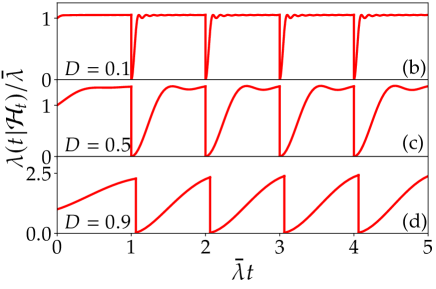
We demonstrate the method by studying the instantaneous emission rate of a single-channel QPC driven by a constant voltage $V$, as illustrated in Fig. 1(a). In this setup, the emission process is stationary. Hence the instantaneous emission rate is independent of $t_{s}$, which can be chosen as $t_{s}=0$. The typical behaviors of $\lambda(t|\mathcal{H}_{t})$ for different QPC transparency $D$ are demonstrated in Fig. 1(b-d). In order to make the discussion concrete, we assume the history $\mathcal{H}_{t}$ corresponds to a sequence of equally spaced time instants, i.e., $\mathcal{H}_{t}=\{t_{1}=1/\bar{\lambda},t_{2}=2/\bar{\lambda},\dots:0<t_{1}<t_{2}<\dots<t\}$. We find that $\lambda(t|\mathcal{H}_{t})$ exhibits discontinuous jumps in all cases: They drop abruptly to zero whenever $t=t_{i}$, indicating the suppression of the emission rate due to the Pauli exclusion principle. After the suppression, the emission rate start to increase, which exhibits different behaviors for different transparency $D$.

In the case of low transparency [Fig 1(b)], the emission rate increases rapidly and saturates to the average emission rate $\bar{\lambda}$. In this case, the correlations between emission events manifest themselves as sharp dips, which can only play a role on short time scales. This makes the emission process can be treated as a simple Poisson process on long time scales, which can be fully characterized by the average emission rate $\bar{\lambda}$. For the QPC with a modest transparency [Fig 1(c)], the increasing of the emission rate is relatively slow. It can reach the saturation value, which is larger then the average emission rate $\bar{\lambda}$. In this case, the dips in the emission rate evolve into wide valleys, indicating that the correlations are non-negligible even on long time scales. Moreover, we find that the $\lambda(t|\mathcal{H}_{t})$ does not depend on the whole history, but is most sensitive to the time instant of the emission of the previous electron. This makes the emission process can be treated approximately as a renewal process, where the correlations are restricted between the two successively emitted electrons. For the QPC with high transparency [Fig 1(d)], the emission rate increases almost linearly as a function of $t$ before the saturation occurs. The saturation value is much larger than the average emission rate $\bar{\lambda}$ and usually cannot be reached in typical cases. As a consequence, the emission rate exhibits a saw-tooth behavior in the time domain, indicating the presence of strong correlations. In this case, the renewal approximation breaks down and the emission process can only be described within the non-renewal theory [10, 12, 13, 8]. These results demonstrate that the conditional intensity function can provide an intuitive and unified description of the electron emission process, which can be used to model both the renewal and non-renewal behaviors.

This paper is organized as follows. First we introduce the basic concept of conditional intensity function in Sec. II. Then we show how to calculate the conditional intensity function for electron emission in Sec. III. We demonstrate the method by studying the electron emission in a dc-biased single-channel QPC in Sec. IV. The relation between the conditional intensity function, WTD and joint WTD are also discussed in this section. Finally, we summarize our results in Sec. V.

II conditional intensity function of a random point process

Suppose one studies the electron emission process via an ideal single-electron detector, then the emission process can be described by recording each emission event in a time trace [See Fig.1(a) for illustration]. This allows us to represent emission events by random points in a line. This is quite similar to the photon emission in quantum optics and neuronal spike emission in neuroscience. Previous studies in these fields show that the emission process can be described by the theory of random point process [14, 11]. Moreover, one usually further assumes that two emission events cannot occur exactly at the same time, i.e., there can only exist at most one emission event in an arbitrary infinitesimal time interval $[t,t+dt)$. The point process satisfied such assumption has been referred to as the regular point process, which has been proved to be a valid assumption for typical emission processes [15, 16, 17, 18].

To characterize the statistics of the emission process, one usually needs a proper probability distribution. In previous studies, the idle time distribution $\Pi(t_{s},t)$ has been introduced [4]. In the theory of random point process, it is also called the survivor function, which is written as $S_{1}(t|t_{s})=\Pi(t_{s},t)$ [11]. It gives the probability that no electron is emitted in the time interval $[t_{s},t]$, where $t_{s}$ can be treated as the starting time of the detector. Alternatively, one can also define the emission probability density $p_{1}(t|t_{s})$, which describes the probability of the electron emission in the infinitesimal interval $[t,t+dt)$ since the staring time $t_{s}$. The two distributions $S_{1}(t|t_{s})$ and $p_{1}(t|t_{s})$ are equivalent, which can be related to each other as

$$S_{1}(t|t_{s})=1-\int^{t}_{t_{s}}d\tau p_{1}(\tau|t_{s}).$$ (1)

By combing these two distributions, one can define a probability intensity function as

$$\lambda_{1}(t|t_{s})=\frac{p_{1}(t|t_{s})}{S_{1}(t|t_{s})}.$$ (2)

This function can be regarded as the conditional emission rate in the infinitesimal interval $[t,t+dt)$, under the condition that no electron is emitted in the time interval $[t_{s},t]$.

The conditional emission rate $\lambda_{1}(t|t_{s})$ essentially represents the emission rate of the first electron since the starting time $t_{s}$. For a history-independent process, it can play the role as the emission rate of the whole process. This can be better illustrated by taking the stationary Poisson point process as an example. The survivor function of the Poisson process can be given as $S_{1}(t|t_{s})=e^{-\lambda_{0}(t-t_{s})}$, with $\lambda_{0}$ being the emission rate. From Eqs. (1) and (2), the corresponding conditional probability can be given as $\lambda_{1}(t|t_{s})=\lambda_{0}$.

The conditional emission rate can be generalized to incorporate the history dependence of the emission process. Consider the emission rate of the $n$-th ($n\geq 2$) electron at time $t$, the corresponding history can be represented by an ordered time sequence $\{t_{1},t_{2},\dots,t_{n-1}\}$, which satisfies

$$t_{s}<t_{1}<t_{2}<\dots<t_{n-1}<t.$$ (3)

Here each $t_{i}$ ($i=1,2,\dots,n-1$) represents the time instant of an electron emission event that has already occurred since the starting time $t_{s}$. To define the conditional emission rate in analogous to Eq. (2), one can generalize the emission probability density $p_{1}(t|t_{s})$ to the conditional emission probability density $p_{n}(t|t_{s},t_{1},t_{2},\dots,t_{n-1})$, which gives the emission probability of the $n$-th electron at the time $t$ under the condition that there have been $n-1$ electrons emitted previously in the infinitesimal interval $[t_{i},t_{i}+dt)$, respectively. The corresponding conditional survivor function can be defined as

$$S_{n}(t|t_{s},t_{1},t_{2},\dots,t_{n-1}) = 1$$ (4)

$${}-\int^{t}_{t_{n-1}}d\tau p_{n}(\tau|t_{s},t_{1},t_{2},\dots,t_{n-1}),$$

which is formally analogous to Eq. (1). Similarly, the conditional emission rate for the $n$-th electron can be given as

$$\lambda_{n}(t|t_{s},t_{1},t_{2},\dots,t_{n-1})=\frac{p_{n}(t|t_{s},t_{1},t_{2},\dots,t_{n-1})}{S_{n}(t|t_{s},t_{1},t_{2},\dots,t_{n-1})}.$$ (5)

Due to the restriction given in Eq. (3), the conditional emission rates $\lambda_{n}(t|t_{s},t_{1},t_{2},\dots,t_{n-1})$ with different $n$ can be merged into one piecewise function $\lambda(t|\mathcal{H}_{t})$, which has the form

$$\lambda(t|\mathcal{H}_{t}) = \begin{cases}\lambda_{1}(t|t_{s}),&t_{s}<t\leq t_{1}\\ \lambda_{2}(t|t_{s},t_{1}),&t_{1}<t\leq t_{2}\\ \lambda_{3}(t|t_{s},t_{1},t_{2}),&t_{2}<t\leq t_{3}\\ \dots\end{cases},$$ (6)

where $\mathcal{H}_{t}=\{t_{1},t_{2},\dots:t_{s}<t_{1}<t_{2}<\dots<t\}$ represents the history of the emission process up to the time $t$. It can be treated as the instantaneous emission rate observed by an ideal single-electron detector since the starting time $t_{s}$. In the theory of random process, it has been referred to as the conditional intensity function [19, 11]. While it is less well-known in the context of mesoscopic transport, it has been extensively used in other fields, such as the study of neuronal spikes in neuroscience and random vibration analysis in civil engineering [14, 18, 11, 20]. With the recent development of machine learning techniques, it can be extracted effectively from the measured waiting times [21, 22], leading to potential applications in the data processing for real-time electron counting techniques [23, 24, 25, 26, 27].

The conditional intensity function provides a time localized description of the emission process, from which the temporal behavior of the emission process can be understood intuitively. Moreover, it also contains the full information of the emission process, from which various statistical quantities can be obtained. In particular, both the WTD and joint WTD can be calculated from the conditional intensity function.

The WTD $\mathcal{W}(t_{s},t_{e})$ is essentially a conditional probability density [28, 3, 29]. It gives the emission probability of the second electron in the infinitesimal interval $[t_{e},t_{e}+dt)$, under the condition that the first electron has already been emitted at the time $t_{s}$. Hence the WTD $\mathcal{W}(t_{s},t_{e})$ can be directly related to the conditional emission probability density $p_{2}(t|t_{s},t_{1})$ as

$$\mathcal{W}(t_{s},t_{e}) = p_{2}(t_{e}|t_{s},t_{s}).$$ (7)

From Eqs. (4) and (5), the conditional emission probability $p_{n}(t|t_{s},t_{1},t_{2},\dots,t_{n-1})$ can be obtained from the conditional emission rates as

$$p_{n}(t|t_{s},t_{1},t_{2},\dots,t_{n-1}) = \lambda_{n}(t|t_{s},t_{1},t_{2},\dots,t_{n-1})$$ (8)

$$\times e^{-\int^{t}_{t_{n-1}}d\tau\lambda_{n}(\tau|t_{s},t_{1},t_{2},\dots,t_{n-1})}.$$

So the WTD $\mathcal{W}(t_{s},t_{e})$ is direct related to the conditional emission rate of the second electron $\lambda_{2}(t_{e}|t_{s},t_{1})$ with $t_{1}=t_{s}$.

Similarly, the joint WTD $\mathcal{W}_{2}(t_{s},t_{m},t_{e})$ can also be obtained from the conditional emission probability density as

$$\mathcal{W}_{2}(t_{s},t_{m},t_{e}) = p_{2}(t_{m}|t_{s},t_{s})p_{3}(t_{e}|t_{s},t_{s},t_{m}).$$ (9)

It gives the emission probability of the third electron in the infinitesimal interval $[t_{e},t_{e}+dt)$, under the condition that the first and second electrons have been emitted at the time $t_{s}$ and $t_{m}$, respectively. So the joint WTD provides additional information on the conditional emission rate of the third electron $\lambda_{3}(t|t_{s},t_{1},t_{2})$ with $t_{1}=t_{s}$ and $t_{2}=t_{m}$. In contrast, the conditional intensity function $\lambda(t|\mathcal{H}_{t})$ from Eq. (6) contains the conditional emission rate of all the $n$ electrons and hence provides a complete description of the whole emission process.

III Electron emission as a determinantal point process

For a general emission process, the conditional intensity function can be calculated directly from the $n$-th order correlation functions [15]. Such calculation is usually rather involved. The calculation can be greatly simplified in the non-interacting case, when all the correlation functions can be expressed as determinants. In this case, the electron emission can be modeled as a determinantal point process [17]. The full information of such process can solely described by the first-order correlation function.

For a single-channel QPC connected to two reservoirs $L$ and $R$ [See Fig. 1(a) for illustration], the first-order correlation function $G(t,t^{\prime})$ corresponding to the electron emission process can be cast into a matrix form [30]

$$G(t,t^{\prime}) = \left[\begin{matrix}G_{RR}(t,t^{\prime})&G_{RL}(t,t^{\prime})\\ G_{LR}(t,t^{\prime})&G_{LL}(t,t^{\prime})\\ \end{matrix}\right]$$ (10)

$$= \langle\Psi|\left[\begin{matrix}\hat{b}^{\dagger}_{R}(t^{\prime})&\hat{b}^{\dagger}_{L}(t^{\prime})\end{matrix}\right]\left[\begin{matrix}\hat{b}_{R}(t)\\ \hat{b}_{L}(t)\\ \end{matrix}\right]|\Psi\rangle$$

$$\mbox{}-\langle F|\left[\begin{matrix}\hat{a}^{\dagger}_{R}(t^{\prime})&\hat{a}^{\dagger}_{L}(t^{\prime})\end{matrix}\right]\left[\begin{matrix}\hat{a}_{R}(t)\\ \hat{a}_{L}(t)\\ \end{matrix}\right]|F\rangle,$$

where $|\Psi\rangle$ represents the many-body state of the emitted electrons, while $|F\rangle$ represents the undisturbed Fermi sea. The incoming and outgoing electrons are represented by Fermion operators $\hat{a}_{\eta}(t)$ and $\hat{b}_{\eta}(t)$ ($\eta=L,R$), respectively. These operators can be related to each other via the scattering matrix as

$$\left[\begin{matrix}\hat{b}_{R}(t)\\ \hat{b}_{L}(t)\\ \end{matrix}\right]=\left[\begin{matrix}\sqrt{1-D}&i\sqrt{D}e^{-i\phi(t)}\\ i\sqrt{D}e^{i\phi(t)}&\sqrt{1-D}\\ \end{matrix}\right]\left[\begin{matrix}\hat{a}_{R}(t)\\ \hat{a}_{L}(t)\\ \end{matrix}\right],$$ (11)

with $D$ representing the transparency of the QPC and $\phi(t)$ being the forward scattering phase.

When the QPC is driven by a constant bias voltage $V$, the forward scattering phase can be expressed as $\phi(t)=eVt/\hbar$. In this case, the first-order correlation function can be decomposed in terms of Martin-Landauer wave packets as

$$\left[\begin{matrix}G_{RR}(t,t^{\prime})&G_{RL}(t,t^{\prime})\\ G_{LR}(t,t^{\prime})&G_{LL}(t,t^{\prime})\\ \end{matrix}\right] = \sum_{l=0,\pm 1,\pm 2,\dots}\left[\begin{matrix}D\psi_{e}(t-lT)\psi^{\ast}_{e}(t^{\prime}-lT)&-i\sqrt{D(1-D)}\psi_{h}(t-lT)\psi^{\ast}_{e}(t^{\prime}-lT)\\ i\sqrt{D(1-D)}\psi_{e}(t-lT)\psi^{\ast}_{h}(t^{\prime}-lT)&D\psi_{h}(t-lT)\psi^{\ast}_{h}(t^{\prime}-lT)\\ \end{matrix}\right],$$ (12)

with $T=h/eV$ representing the repetition period and

$$\psi_{e}(t) = \frac{1}{\sqrt{T}}e^{-i\pi t/T}\frac{\sin(\pi t/T)}{\pi t/T},$$

$$\psi_{h}(t) = \frac{1}{\sqrt{T}}e^{i\pi t/T}\frac{\sin(\pi t/T)}{\pi t/T},$$ (13)

representing the Martin-Landauer wave packets corresponding to the emitted electrons and holes, respectively.

From the above expression, one can see that the four components of the first-order correlation function $G_{\eta\eta^{\prime}}(t,t^{\prime})$ have different physical meanings: $G_{RR}(t,t^{\prime})$ [$G_{LL}(t,t^{\prime})$] describes the emission of electrons [holes] into the right [left] reservoir. In contrast, $G_{LR}(t,t^{\prime})$ [$G_{RL}(t,t^{\prime})$] corresponds to the emission of electron-hole pairs: While the electron [hole] component is emitted to the left [right] reservoir, the hole [electron] component is reflected back to the right [left] reservoir.

In this paper, we focus on the electron emission into the right reservoirs, which corresponds to the component $G_{RR}(t,t^{\prime})$. To calculate the conditional intensity function by using Eqs. (4) and (5), one needs information of the survivor function $S_{n}(t|t_{s},t_{1},t_{2},\dots,t_{n-1})$ or the conditional emission probability $p_{n}(t|t_{s},t_{1},t_{2},\dots,t_{n-1})$. In a previous work, Macchi has shown that they can be extracted from $G_{RR}(t,t^{\prime})$ via the following procedure [17]:

• Solve the eigenvalue equation:

  $$\int^{t}_{t_{s}}d\tau^{\prime}G_{RR}(\tau,\tau^{\prime})\varphi_{\alpha}(\tau^{\prime})=\nu_{\alpha}\varphi_{\alpha}(\tau),$$ (14)

  with $\alpha=1,2,\dots$ being the index of the eigenvalues and eigenfunctions. The eigenvalue $\nu_{\alpha}$ satisfies $0\leq\nu_{\alpha}\leq 1$, while the eigenfunctions $\varphi_{\alpha}(\tau)$ form an orthonormal basis within the time interval $[t_{s},t]$, i.e.,

  $$\int^{t}_{t_{s}}d\tau\varphi^{\ast}_{\alpha}(\tau)\varphi_{\alpha^{\prime}}(\tau)=\delta_{\alpha,\alpha^{\prime}}.$$ (15)

  From the eigenvalues and eigenfunctions, one can define an auxiliary function as

  $$C(t,t^{\prime})=\sum_{\alpha=1}^{+\infty}\frac{\nu_{\alpha}}{1-\nu_{\alpha}}\varphi_{\alpha}(t)\varphi^{\ast}_{\alpha}(t^{\prime}).$$ (16)

• Define the exclusive density function $\pi_{n}(t_{1},t_{2},\dots,t_{n}|t_{s},t)$ as

  $$\pi_{n}(t_{1},t_{2},\dots,t_{n}|t_{s},t) = p_{1}(t_{1}|t_{s})$$ (17)

  $$\times p_{2}(t_{2}|t_{s},t_{1})\cdots p_{n}(t_{n}|t_{s},t_{1},\dots,t_{n-1})$$

  $$\times S_{n+1}(t|t_{s},t_{1},t_{2},\dots,t_{n}),$$

  with $n\geq 1$. This function can be calculated from $C(t,t^{\prime})$ and $\nu_{\alpha}$ as

  $$\pi_{n}(t_{1},t_{2},\dots,t_{n}|t_{s},t)=\Big{[}\prod_{\alpha=1}^{N}(1-\nu_{\alpha})\Big{]}$$

  $$\times\begin{vmatrix}C(t_{1},t_{1})&C(t_{1},t_{2})&\dots&C(t_{1},t_{n})\\ C(t_{2},t_{1})&C(t_{2},t_{2})&\dots&C(t_{2},t_{n})\\ {1}\\ C(t_{n},t_{1})&C(t_{n},t_{2})&\dots&C(t_{n},t_{n})\end{vmatrix}.$$ (18)

• The corresponding idle time distribution $\Pi(t_{s},t)$, or equivalently the survivor function $S_{1}(t|t_{s})$, can be solely determined by the $\nu_{\alpha}$ as

  $$\Pi(t_{s},t)=S_{1}(t|t_{s})=\prod_{\alpha=1}^{N}(1-\nu_{\alpha}).$$ (19)

  Equation (18) and (19) can be used to extract $S_{n}(t|t_{s},t_{1},t_{2},\dots,t_{n-1})$ and $p_{n}(t|t_{s},t_{1},t_{2},\dots,t_{n-1})$.

Then all the conditional emission rates $\lambda_{n}(t|t_{s},t_{1},t_{2},\dots,t_{n-1})$ can be calculated by using Eqs. (1), (2), (4) and (5). For example, the conditional emission rate for the first and second electrons can be written as

$$\lambda_{1}(t|t_{s}) = C(t,t),$$ (20)

$$\lambda_{2}(t|t_{s},t_{1}) = \frac{C(t_{1},t_{1})C(t,t)-\left|C(t_{1},t)\right|^{2}}{C(t,t)}.$$ (21)

This provides an efficient numerical methods to evaluate the conditional intensity function given in Eq. (6).

It is worth noting that the eigenvalue $\nu_{\alpha}$ obtained from Eq. (14) can be treated as the emission probability of the $\alpha$-th electron emitted in the time interval $[t_{s},t]$. This can be seen from the time-dependent full counting statistics (FCS). The corresponding momentum generating function of the FCS can be given as [17]

$$\Phi(\chi)=\prod_{\alpha=1}^{+\infty}\left(1-\nu_{\alpha}+e^{i\chi}\nu_{\alpha}\right).$$ (22)

This corresponds to a generalized binomial statistics, which indicates that within a finite time interval $[t_{s},t]$, the $\alpha$-th electron attempts to emit with a success probability $\nu_{\alpha}$. Note that the probability $\nu_{\alpha}$ is not a constant, but typically time-dependent. Hence the corresponding emission events should not be considered as independent Bernoulli trials, but are time-correlated.

General speaking, all the results should also depends on the starting time $t_{s}$. This is is irrelevant for the dc-biased QPC, as the emission process is stationary. Without loss of generality, in the following discussion we always choose $t_{s}=0.0$. In this case, the WTD and joint WTD from Eqs. (7) and (9) can be written as

$$\mathcal{W}(\tau) = \mathcal{W}(t_{s},t_{s}+\tau),$$ (23)

$$\mathcal{W}_{2}(\tau_{1},\tau_{2}) = \mathcal{W}_{2}(t_{s},t_{s}+\tau_{1},t_{s}+\tau_{1}+\tau_{2}).$$ (24)

IV Emission rates for QPC

From the discussion in the above section, one can see that, for a dc-biased QPC, the emitted electrons can be represented by a sequence of Martin-Landauer wave packets with repetition period $T$, which can transmit across the QPC with a finite probability $D$. The average emission rate of the electron can then be given as $\bar{\lambda}=D/T$. Here the repetition period $T=h/eV$ is decided by the bias voltage, while the probability $D$ is just equal to the QPC transparency. The two parameters $T$ and $D$ have different impacts on the emission process.

Figure 2: Emission probabilities $\nu_{\alpha}$ as functions of time $t$. The horizontal line is restricted to the QPC transparency $D$.

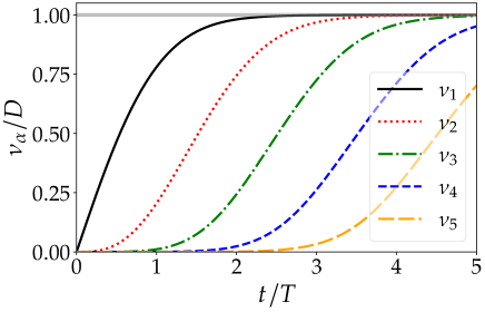
To see this, let us first concentrate on the emission probabilities $\nu_{\alpha}$. From Eqs. (12), (13) and (14), one can see that the time-dependence of $\nu_{\alpha}$ is mainly decided by the repetition period $T$. Indeed, as the time $t$ increases, all the emission probabilities increase monotonically and saturate on timescales comparable to $T$. This is illustrated in Fig. 2. In contrast, the QPC transparency $D$ merely plays the role of a scale factor, which only restricts the saturation value of the emission probabilities to $D$ [illustrated by the grey line in Fig. 2].

Figure 3: (a) The conditional emission rate of the first electron $\lambda_{1}(t|0)$ (b) The conditional emission rate of the second electron $\lambda_{2}(t|0,T)$. In both figures, curves with different curves with different colors and line types correspond to different QPC transparency $D$.

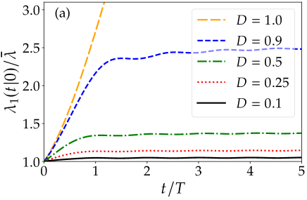
Although the impact of $D$ on the emission probabilities is trivial, it has a much pronounced impact on the emission rates. This can be seen from the conditional emission rate $\lambda_{1}(t|0)$ of the first electron, which is illustrated in Fig. 3(a). In the figure, curves with different colors and line types correspond to $\lambda_{1}(t|0)$ with different transparency $D$. At the time $t/T=0.0$, $\lambda_{1}(t|0)$ is equal to the average emission rate $\bar{\lambda}$. As $t$ increases, it start to increase, which shows different behaviors for different $D$: For $D<1.0$, $\lambda_{1}(t|0)$ saturates on the timescale of $T$ and undergoes a weak oscillation around the saturation value as $t$ further increases. This can be seen from the black solid, red dotted, green dash-dotted and blue dashed curves, corresponding to $D=0.1$, $0.25$, $0.5$ and $0.9$, respectively. In contrast, $\lambda_{1}(t|0)$ does not saturate at all for $D=1.0$. It increases almost linearly as a function of $t$, which is illustrated by the orange long dashed curve in the figure.

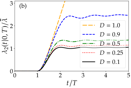
Similar behaviors can also be found for other conditional emission rates. To demonstrate this, we plot the conditional emission rate of the second electron $\lambda_{2}(t|0,T)$ in Fig. 3(b). Curves with different colors and line types correspond to $\lambda_{2}(t|0,T)$ with different transparency $D$. From the figure, one always finds $\lambda_{2}(t|0,T)=0.0$ for $t=T$, indicating that the emission of the second electron is hindered by the first electron emitted at the time instant $t_{1}=T$. For $D<1.0$, $\lambda_{2}(t|0,T)$ increases as a function of $t$ and saturates before $t/T=2.0$. Then it undergoes a weak oscillation around the saturation value as $t$ further increases. These behaviors are illustrated by the black solid, red dotted, green dash-dotted and blue dashed curves, corresponding to $D=0.1$, $0.25$, $0.5$ and $0.9$, respectively. For $D=1.0$, $\lambda_{2}(t|0,T)$ increases almost linearly as a function of $t$ and does not saturate at all. This can be seen from the orange long dashed curve. These results indicates that the rising time of the conditional emission rates are decided solely by the repetition period $T$.

The conditional intensity function $\lambda(t|\mathcal{H}_{t})$ can be obtained by combining all the conditional emission rates following Eq. (6). To do this, one needs to choose a proper set of $t_{i}$, which represents the time instants of emission events in the history $\mathcal{H}_{t}$ [see the definition of $\mathcal{H}_{t}$ below Eq. (6)]. Due to the probabilistic nature of the electron emission, $t_{i}$ are essentially random parameters. Their waiting times $\tau=t_{i}-t_{i-1}$ follow the WTD $\mathcal{W}(\tau)$, whose mean value is equal to the average waiting time $1/\bar{\lambda}$. In order to simplify the discussion, we choose $t_{i}=i/\bar{\lambda}$ in the following calculation.

Figure 4: (a) Conditional emission rates $\lambda_{n}(t|0,t_{1},t_{2},\dots,t_{n-1})$ for the first five electrons. The black solid, red dotted, green dash-dotted, blue dashed, and orange long-dashed curves correspond to $n=1,2,3,4$ and $5$, respectively. (b) The conditional intensity function $\lambda(t|\mathcal{H}_{t})$ obtained from the conditional emission rates via Eq. (6). The average emission rate $\bar{\lambda}$ is plotted by the horizontal grey line. All the emission rates and $t$ are rescaled according to the average emission rate $\bar{\lambda}$.

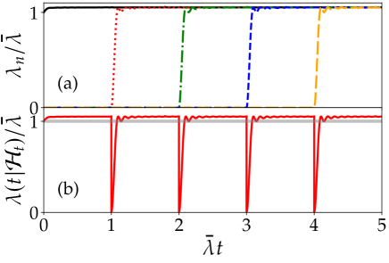
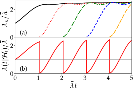
In the case of low transparency, the rising time of the conditional emission rates is much shorter than the average waiting time. This case is demonstrated in Fig. 4, corresponding to $D=0.1$. In Fig. 4(a), we plot the conditional emission rates for the first five emitted electrons with different curves. Due to the short rising time, one can see that the emission rate can exhibit a step-like increase around the time $t=t_{i}$. The oscillation around the saturation value is also rather small. This makes the corresponding conditional intensity function can be well-approximated by the average emission rate $\bar{\lambda}$ in most regions, as illustrated in Fig. 4(b). The approximation is only invalid at the vicinity of $t_{i}$, where the conditional intensity function exhibits sharp dips. These dips is not crucial for long-time properties, such as dc shot noise. This makes the electron emission can be treated approximated as a simple Poisson process on long time scales, which can be characterized via a constant emission rate.

Figure 5: Main panel: Conditional emission rates $\lambda_{n}(t|0,t_{1},t_{2},\dots,t_{n-1})$ as a function of the waiting time $t-t_{n-1}$. The red solid, green dotted, blue dash-dotted, and orange dashed curves correspond to $n=2,3,4$ and $5$, respectively. Note that all the curves are highly overlapped. Inset: Rescaled WTD $\mathcal{W}(\tau)/\bar{\lambda}$ and joint WTD $\mathcal{W}_{2}(\tau_{1},\tau)/[\mathcal{W}(\tau_{1})\bar{\lambda}]$ as functions of $\bar{\lambda}\tau$. The grey dotted curve in the inset corresponds to the WTD of the simple Poisson process.

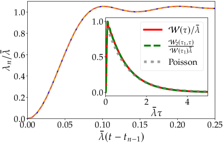
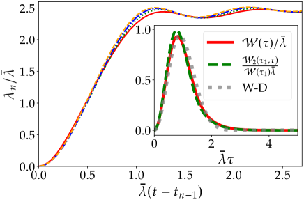
As long as short-time behaviors are concerned, the Poisson approximation breaks down. In this case, one has to characterize the emission rate via the conditional intensity function $\lambda(t|\mathcal{H}_{t})$, which generally has a complicated history-dependence. However, in the case of low transparency, we find that the conditional emission rate $\lambda_{n}(t|0,t_{1},t_{2},\dots,t_{n-1})$ do not depend on the whole history $\mathcal{H}_{t}$, but is only sensitive to the time instant of the emission of the previous electron. As a consequence, all the conditional emission rates have a similar profile as a function of the waiting time $t-t_{n-1}$. This is illustrated in the main panel of Fig. 5. In the figure, we plot the conditional emission rate $\lambda_{n}(t|0,t_{1},t_{2},\dots,t_{n-1})$ as the function of $t-t_{n-1}$, where the red solid, green dotted, blue dash-dotted, and orange dashed curves correspond to $n=2,3,4$ and $5$, respectively. One can see that all the curves coincide with each other. This indicates that they can be expressed as $\lambda_{n}(t|0,t_{1},t_{2},\dots,t_{n-1})=\lambda_{r}(t-t_{n-1})$, which essentially corresponds to a stationary renewal process.

The renewal behavior can also be seen from the joint WTD analysis. For a renewal process, one expects that $\mathcal{W}_{2}(\tau_{1},\tau_{2})=\mathcal{W}(\tau_{1})\mathcal{W}(\tau_{2})$, indicating that there are no correlation between waiting times. To demonstrate this, we plot the rescaled WTD $\mathcal{W}(\tau)/\bar{\lambda}$ [calculated from Eqs. (7), (8) and (23)] by the red solid curve in the inset of Fig. 5. The corresponding rescaled joint WTD $\mathcal{W}_{2}(\tau_{1},\tau)/[\mathcal{W}(\tau_{1})\bar{\lambda}]$ is plotted with the green dotted curves, where we have chosen $\tau_{1}=1/\bar{\lambda}$. One can see that two curves agree quite well, indicating the absence of the correlation between waiting times. Moreover, one can see that both WTDs can be well-approximated by an exponential distribution (grey curve) for large $\tau$, indicating that the process can be treated as a simple Poisson process on long time scales.

Figure 6: The same as Fig. 4, but with $D=0.5$.

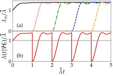
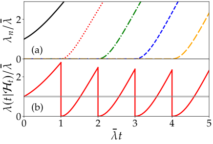
For the QPC with modest transparency, the rising time of the conditional emission rates can be comparable to the average waiting time. This case is demonstrated in Fig. 6(a), corresponding to $D=0.5$. Due to the long rising time, the dips evolves into wide valleys. Moreover, the saturation value is also much larger then the average emission rate. One can also see a pronounced oscillation in the saturation region. These features can be seen from Fig. 6(b). All these features indicates that the emission process cannot be approximated as a stationary Poisson process even on long time scales. However, we find that all the conditional emission rates $\lambda_{n}(t|0,t_{1},t_{2},\dots,t_{n-1})$ as a function of the waiting time $t-t_{n-1}$ still have a similar profile, which is illustrated in the main panel of Fig. 7. This indicates that the emission process can still be treated as a renewal process.

Figure 7: The same as Fig. 5, but with $D=0.5$.

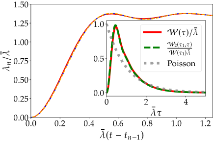
The renewal behavior can also be seen from the WTD analysis, which is illustrated in the inset of Fig. 7. As the two rescaled WTDs coincides, the join WTD can still be approximated as $\mathcal{W}_{2}(\tau_{1},\tau)=\mathcal{W}(\tau_{1})\mathcal{W}(\tau)$, indicating the absence of correlation between waiting times. Note that the profile of the WTDs are significantly different from an exponential distribution, indicating a departure from the Poisson approximation.

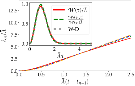
As the QPC is further opened up, the rising time of the conditional emission rates can be longer than the average waiting time. This case is demonstrated in Fig. 8(a), corresponding to $D=0.9$. In this case, the conditional intensity function exhibits a saw-tooth behavior in the time domain, indicating the presence of strong correlations. This makes the renewal approximation breaks down: The conditional emission rates for different electrons can exhibit different time dependence, which cannot be described by a universal rate function $\lambda_{r}(t-t_{n-1})$. This is demonstrated in the main panel of Fig. 9. Accordingly, the relation $\mathcal{W}_{2}(\tau_{1},\tau)=\mathcal{W}(\tau_{1})\mathcal{W}(\tau)$ does not hold, which is plotted in the inset of Fig. 9. Note that the WTD in this case is quite close to the Wigner-Dyson distribution, which is plotted by the grey dotted curve in the inset.

The correlation is most pronounced as the QPC is fully opened. This is demonstrated in Fig. 10 and 11, corresponding to $D=1.0$. In this case, all the conditional emission rates do not saturate at all. They increase almost linearly as functions of $t$, which is plotted in the main panel of Fig. 11. Note that in this case, the corresponding WTD fully agrees with the Wigner-Dyson distribution, which can be seen by comparing the red solid curve to the grey dotted curve in the inset of Fig. 11.

Figure 8: The same as Fig. 4, but with $D=0.9$.

Figure 9: The same as Fig. 5, but with $D=0.9$. The grey dotted curve in the inset corresponds to the Wigner-Dyson distribution.

Figure 10: The same as Fig. 4, but with $D=1.0$.

Figure 11: The same as Fig. 5, but with $D=1.0$. The grey dotted curve in the inset corresponds to the Wigner-Dyson distribution.

V Conclusion

We have shown that the electron emission rate through a quantum point contact can be described by using the conditional intensity function $\lambda(t|\mathcal{H}_{t})$. For non-interacting systems, the conditional intensity function $\lambda(t|\mathcal{H}_{t})$ can be obtained from the first-order correlation function. It provides an intuitive way to understand the temporal behavior of the emission process. As the QPC is close to pinch-off, the conditional intensity function $\lambda(t|\mathcal{H}_{t})$ can be well-approximated by a constant emission rate $\bar{\lambda}$ in most regions. This indicates that the emission process can be treated as a simple Poisson process on long time scales. The correlations between electron emissions manifests themselves as sharp dips in the conditional intensity function $\lambda(t|\mathcal{H}_{t})$, which can only play a role on short time scales. As the QPC is opened up, the correlations become more and more important. For QPC with modest transparency, the dips due to the correlation evolve into wide valleys, which become non-negligible even on long time scales. In this case, the emission process can be treated approximately as a renewal process, whose statistics behaviors can be solely decided via the WTD $\mathcal{W}(\tau)$. For QPC with high transparency, the correlations are so strong that the conditional intensity function $\lambda(t|\mathcal{H}_{t})$ exhibits a saw-tooth behavior. In this case, the emission process can only be described within the non-renewal theory. These results indicates that the conditional intensity function $\lambda(t|\mathcal{H}_{t})$ provides a unified description of the emission process, which can be used to model both the renewal and non-renewal behaviors.

References

- Levitov et al. [1996] L. S. Levitov, H. Lee, and G. B. Lesovik, Journal of Mathematical Physics 37, 4845 (1996).
- Blanter and Büttiker [1999] Y. Blanter and M. Büttiker, Physics Reports 336, 1 (1999).
- Brandes [2008] T. Brandes, Annalen der Physik 17, 477 (2008).
- Albert et al. [2012] M. Albert, G. Haack, C. Flindt, and M. Büttiker, Physical Review Letters 108, 186806 (2012).
- Haack et al. [2014] G. Haack, M. Albert, and C. Flindt, Physical Review B 90, 205429 (2014).
- Hofer et al. [2015] P. P. Hofer, D. Dasenbrook, and C. Flindt, Physica E: Low-dimensional Systems and Nanostructures 82, 3 (2015).
- Ptaszyński [2017] K. Ptaszyński, Physical Review B 95, 045306 (2017).
- Rudge and Kosov [2019] S. L. Rudge and D. S. Kosov, Physical Review B 99, 115426 (2019).
- Kleinherbers et al. [2021] E. Kleinherbers, P. Stegmann, and J. König, Physical Review B 104, 165304 (2021).
- Dasenbrook et al. [2015] D. Dasenbrook, P. P. Hofer, and C. Flindt, Physical Review B 91, 195420 (2015).
- D. J. Daley [2003] D. V.-J. D. J. Daley, An Introduction to the Theory of Point Processes (Springer New York, 2003).
- Ptaszynski [2017] K. Ptaszynski, Physical Review B 96, 035409 (2017).
- Kosov [2017] D. S. Kosov, The Journal of Chemical Physics 147, 104109 (2017).
- Snyder and Miller [1991] D. L. Snyder and M. I. Miller, Random Point Processes in Time and Space (Springer New York, 1991).
- Kelley and Kleiner [1964] P. L. Kelley and W. H. Kleiner, Physical Review 136, A316 (1964).
- Mandel and Wolf [1965] L. Mandel and E. Wolf, Reviews of Modern Physics 37, 231 (1965).
- Macchi [1975] O. Macchi, Advances in Applied Probability 7, 83 (1975).
- Iwankiewicz [1995] R. Iwankiewicz, Dynamical Mechanical Systems Under Random Impulses (World Scientific Publishing London, 1995).
- Cox [1962] D. R. Cox, Renewal Theory (Methuen, London, 1962).
- Kass et al. [2014] R. E. Kass, U. T. Eden, and E. N. Brown, Analysis of Neural Data (Springer New York, 2014).
- Du et al. [2016] N. Du, H. Dai, R. Trivedi, U. Upadhyay, M. Gomez-Rodriguez, and L. Song, in Proceedings of the 22nd ACM SIGKDD International Conference on Knowledge Discovery and Data Mining (ACM, 2016).
- Eichler et al. [2016] M. Eichler, R. Dahlhaus, and J. Dueck, Journal of Time Series Analysis 38, 225 (2016).
- Gustavsson et al. [2009] S. Gustavsson, R. Leturcq, M. Studer, I. Shorubalko, T. Ihn, K. Ensslin, D. Driscoll, and A. Gossard, Surface Science Reports 64, 191 (2009).
- Maisi et al. [2011] V. F. Maisi, O. P. Saira, Y. A. Pashkin, J. S. Tsai, D. V. Averin, and J. P. Pekola, Physical Review Letters 106, 217003 (2011).
- Kurzmann et al. [2019] A. Kurzmann, P. Stegmann, J. Kerski, R. Schott, A. Ludwig, A. D. Wieck, J. König, A. Lorke, and M. Geller, Physical Review Letter 122, 247403 (2019).
- Ranni et al. [2021] A. Ranni, F. Brange, E. T. Mannila, C. Flindt, and V. F. Maisi, Nature Communications 12, 6358 (2021).
- Brange et al. [2020] F. Brange, A. Schmidt, J. C. Bayer, T. Wagner, C. Flindt, and R. J. Haug, Science Advances 7 (2020).
- Vyas and Singh [1988] R. Vyas and S. Singh, Physical Review A 38, 2423 (1988).
- Albert et al. [2011] M. Albert, C. Flindt, and M. Büttiker, Physical Review Letters 107, 086805 (2011).
- Haack et al. [2012] G. Haack, M. Moskalets, and M. Büttiker, Physical Review B 87, 201302 (2012).