Graph Pooling for Graph Neural Networks: Progress, Challenges, and Opportunities

Abstract

Graph neural networks have emerged as a leading architecture for many graph-level tasks, such as graph classification and graph generation. As an essential component of the architecture, graph pooling is indispensable for obtaining a holistic graph-level representation of the whole graph. Although a great variety of methods have been proposed in this promising and fast-developing research field, to the best of our knowledge, little effort has been made to systematically summarize these works. To set the stage for the development of future works, in this paper, we attempt to fill this gap by providing a broad review of recent methods for graph pooling. Specifically, 1) we first propose a taxonomy of existing graph pooling methods with a mathematical summary for each category; 2) then, we provide an overview of the libraries related to graph pooling, including the commonly used datasets, model architectures for downstream tasks, and open-source implementations; 3) next, we further outline the applications that incorporate the idea of graph pooling in a variety of domains; 4) finally, we discuss certain critical challenges facing current studies and share our insights on future potential directions for research on the improvement of graph pooling.

1 Introduction

Graph Neural Networks (GNNs) have achieved a substantial improvement over many graph-level tasks such as graph classification Errica et al. (2020), graph regression Bianchi et al. (2020a), and graph generation Baek et al. (2021). Specifically, GNNs have been successfully applied to graph-level tasks across a broad range of areas such as chemistry and biology Baek et al. (2021), social network Ma et al. (2021), computer vision Fey et al. (2018), natural language processing Gao et al. (2019), and recommendation Wu et al. (2021).

Different from node-level tasks, which mainly use the graph convolutional network (GCN) Kipf and Welling (2017) to generate node representations for downstream tasks, graph-level tasks require holistic graph-level representations for graph-structured inputs whose size and topology are varying. Therefore, for graph-level tasks, the pooling mechanism is an essential component, which condenses the input graph with node representations generated by GCN into a smaller sized graph or a single vector, as shown in Figure 1.

In order to obtain an effective and reasonable graph representation, many designs of graph pooling have been proposed, which could be roughly divided into Flat Pooling (Section 3.1) and Hierarchical Pooling (Section 3.2). The former directly generates a graph-level representation in one step, mostly taking the average or sum over all node embeddings as the graph representation Duvenaud et al. (2015), while the latter coarsens a graph gradually into a smaller sized graph by two main means: Node Clustering Pooling and Node Drop Pooling. Specifically, node clustering pooling Ying et al. (2018) groups nodes into clusters as a coarsened graph, which is time-and space-consuming Bianchi et al. (2020a). In contrast, node drop pooling Gao and Ji (2019) selects a subset of nodes from the original graph to construct a coarsened graph, which is more efficient and more suitable for large-scale graphs Lee et al. (2019) but suffers from inevitable information loss Gao et al. (2021b).

Although such state-of-the-art graph pooling methods have been proposed, only a few recent works have attempted to comprehensively evaluate the effects of graph pooling Mesquita et al. (2020); Grattarola et al. (2021), and a systematic review of the progress of and challenges facing this emerging area is still lacking. To fill the gaps, we comprehensively survey graph pooling in this paper, including proposing a taxonomy and formulating relevant frameworks (Section 3), overviewing libraries (Section 4), outlining applications (Section 5), and discussing future research directions (Section 6). To the best of our knowledge, our paper is the first attempt to present a systematic and comprehensive review of recent progress on graph pooling. The purpose of this paper is to provide new practitioners with a comprehensive understanding of graph pooling and to keep researchers informed about the latest advancements in this field.

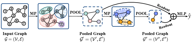
Figure 1: An illustrative example of graph pooling. Here, MP refers to message passing, and POOL refers to the pooling function.

2 Problem Formulation

Notions.

Let $\mathcal{G}=(\mathcal{V},\mathcal{E})$ denote a graph with node set $\mathcal{V}$ and edge set $\mathcal{E}$. Node features are denoted as $\bm{X}\in\mathbb{R}^{n\times d}$, where $n$ is the number of nodes, and $d$ is the dimension of node features. The adjacency matrix is defined as $\bm{A}\in\{0,1\}^{n\times n}$. $\bm{A}[i,j]=1$ if there exists an edge between node $v_{i}$ and node $v_{j}$, otherwise, $\bm{A}[i,j]=0$.

Graph Pooling.

Let a graph pooling operator be defined as any function $\operatorname{POOL}$ that maps a graph $\mathcal{G}$ to a new pooled graph $\mathcal{G}^{\prime}=(\mathcal{V}^{\prime},\mathcal{E}^{\prime})$ :

$$\mathcal{G}^{\prime}=\operatorname{POOL}(\mathcal{G}),$$ (1)

where $|\mathcal{V}^{\prime}|<|\mathcal{V}|$ . The primary goal of graph pooling is to reduce the number of nodes in a graph while preserving the semantic information of the graph.

3 Approaches for Graph Pooling

Graph pooling can be roughly divided into flat pooling and hierarchical pooling according to its role in graph-level representation learning. The former directly generates graph-level representations in a single step ($|\mathcal{V}^{\prime}|=1$), while the latter coarsens the graph gradually into a smaller sized graph ($|\mathcal{V}^{\prime}|>1$).

3.1 Flat Pooling

Flat pooling, also known as graph readout operation, directly generates a graph-level representation $\bm{h}_{G}$ in one step. Thus, Eq. 1 in the case of flat pooling can be denoted as:

$$\bm{h}_{G}=\operatorname{POOL}_{\text{flat}}(\mathcal{G}),$$ (2)

where $\operatorname{POOL}_{\text{flat}}$ denotes the graph pooling function, which must: 1) output fixed-sized graph representations when input graphs are of different sizes; 2) output the same representation when the order of nodes of an input graph changes.

In light of the above discussions, several designs of flat pooling layers have been proposed. The most commonly used method is the sum-pool or mean-pool, which performs averaging or summing operations over all node representations Duvenaud et al. (2015); Xu et al. (2019). Some methods Navarin et al. (2019); Chen et al. (2019); Papp et al. (2021) perform an additional non-linearity transformation to improve the expressive power of pooling methods. Moreover, some methods Li et al. (2016); Atwood and Towsley (2016); Bai et al. (2019); Fan et al. (2020); Itoh et al. (2022) introduce the soft attention mechanism to determine the weight of each vertex in the final graph-level representation. Besides, some methods Zhang et al. (2018); Bai et al. (2021) apply convolutional neural networks to sorted node representations. Different from the above methods, which collect the first-order statistic information of node representations, SOPool, proposed by Wang et al. Wang and Ji (2020), considers the important second-order statistics, which refers to functions that utilize the second power of node features. Furthermore, DKEPool Chen et al. (2022) takes into consideration the entire node distribution of a graph. Due to space limitation, some other flat pooling methods such as Set2set Vinyals et al. (2016), DEMO-Net Wu et al. (2019), SSRead Lee et al. (2021), and GMT Baek et al. (2021) are not presented here.

Most of the above flat pooling methods perform operations on node representations to obtain graph-level representations without consideration of the intrinsic hierarchical structures of graphs, which causes information loss and degrades the performance of graph representations Knyazev et al. (2019); Bianchi and Lachi (2023).

3.2 Hierarchical Pooling

Hierarchical pooling methods aim to preserve the hierarchical graph’s structural information by iteratively coarsening the graph into a new graph in smaller size. The hierarchical pooling can be roughly classified into node clustering pooling, node drop pooling, and other pooling according to the manner in which it coarsens a graph. The main difference between the first two types of methods is that node clustering pooling generates new nodes for the coarsened graph, whereas node drop pooling retains nodes from the original graph. Note that hierarchical pooling methods still technically employ flat pooling methods (readout in Figure 1) to obtain the graph-level representation of the coarsened graph.

[b]       Models       CAM Generator       Graph Coarsening       Notes              DiffPool^[1]       $\bm{C}=\operatorname{softmax}(\operatorname{GNN}_{\text{pool}}(\bm{X},\bm{A}))$       $\left\{\begin{aligned} &\bm{X}^{\prime}=\bm{C}^{T}\cdot\operatorname{GNN}_{\text{emb}}(\bm{X},\bm{A})\\ &\bm{A}^{\prime}=\bm{C}^{T}\bm{A}\bm{C}\\ \end{aligned}\right.$       Auxiliary Loss ^{\raisebox{-0.9pt}{1}⃝}              NMF^[2]       $\left\{\begin{aligned} &\bm{A}\approx\bm{U}\bm{V}\\ &\bm{C}=\bm{V}^{T}\end{aligned}\right.$       $\bm{X}^{\prime}=\bm{C}^{T}\bm{X};\bm{A}^{\prime}=\bm{C}^{T}\bm{A}\bm{C}$       –              LaPool^[3]       $\left\{\begin{aligned} &s_{i}=\|\sum_{j\in\mathcal{N}\left(v_{i}\right)}A_{i,j}\left(\mathbf{x}_{i}-\mathbf{x}_{j}\right)\|_{2}\\ &\mathcal{V}_{c}=\left\{v_{i}\in\mathcal{V}\mid\forall v_{j},s_{i}-\bm{A}_{ij}s_{j}>0\right\}\\ &\bm{C}=\operatorname{sparsemax}\left(\mathbf{p}\frac{\bm{XX}_{c}^{T}}{\|\bm{X}\|\left\|\bm{X}_{c}\right\|}\right)\end{aligned}\right.$       $\left\{\begin{aligned} &\bm{X}^{\prime}=\operatorname{MLP}(\bm{C}^{T}\bm{X})\\ &\bm{A}^{\prime}=\bm{C}^{T}\bm{A}\bm{C}\\ \end{aligned}\right.$       –              MinCut^[4]       $\bm{C}=\operatorname{MLP}(\bm{X})$       $\left\{\begin{aligned} &\bm{X}^{\prime}=\bm{C}^{T}\bm{X};\widehat{\bm{A}}=\bm{C}^{T}\widetilde{\bm{A}}\bm{C}\\ &\bm{A}^{\prime}=\widehat{\bm{A}}-\bm{I}\text{diag}(\widehat{\bm{A}})\end{aligned}\right.$       MinCut Loss ^{\raisebox{-0.9pt}{2}⃝}              StructPool^[5]       $\bm{C}:\operatorname{Minimiz}E(\bm{C})$ ^{\raisebox{-0.9pt}{3}⃝}       $\bm{X}^{\prime}=\bm{C}^{T}\bm{X};\bm{A}^{\prime}=\bm{C}^{T}\bm{A}\bm{C}$       –              MemPool^[6]       $\left\{\begin{aligned} &\bm{C}_{i,j}=\frac{\left(1+\left\|\mathbf{x}_{i}-\mathbf{k}_{j}\right\|^{2}/\tau\right)^{-\frac{\tau+1}{2}}}{\sum_{j^{\prime}}\left(1+\|\mathbf{x}_{i}-\mathbf{k}_{j^{\prime}}\|^{2}/\tau\right)^{-\frac{\tau+1}{2}}}\\ &\bm{C}=\operatorname{softmax}\left(\Gamma\left(\overset{|m|}{\underset{t=0}{\|}}\bm{C}_{t}\right)\right)\end{aligned}\right.$       $\bm{X}^{\prime}=\operatorname{MLP}(\bm{C}^{T}\bm{X})$       Auxiliary Loss ^{\raisebox{-0.9pt}{4}⃝}              HAP^[7]       $\left\{\begin{aligned} &\bm{T}=\operatorname{GCont}(\bm{X})\\ &\bm{C}_{ij}=\sigma\left(\mathbf{p}^{T}[\bm{T}_{\text{Row}_{i}}\|\bm{T}_{\text{Col}_{j}}]\right)\\ &\bm{C}=\operatorname{softmax}(\bm{C})\end{aligned}\right.$       $\left\{\begin{aligned} &\bm{X}^{\prime}=\operatorname{MLP}(\bm{C}^{T}\bm{X}),\widehat{\bm{A}}=\bm{C}^{T}\bm{A}\bm{C}\\ &\bm{A}^{\prime}=\operatorname{Gumbel-SoftMax}(\widehat{\bm{A}})\\ \end{aligned}\right.$       –              SEP^[8]       $\bm{C}:\operatorname{Minimiz}\mathcal{H}^{T}(\mathcal{G})$ ^{\raisebox{-0.9pt}{5}⃝}       $\bm{X}^{\prime}=\bm{C}^{T}\bm{X};\bm{A}^{\prime}=\bm{C}^{T}\bm{A}\bm{C}$       – ^[1]Ying et al. (2018); ^[2]Bacciu and Sotto (2019); ^[3]Noutahi et al. (2019); ^[4]Bianchi et al. (2020a); ^[5]Yuan and Ji (2020); ^[6]Khasahmadi et al. (2020); ^[7]Liu et al. (2021a); ^[7]Wu and others (2022) \raisebox{-0.9pt}{1}⃝ Auxiliary loss consists of the link prediction objective loss and entropy regularization loss. \raisebox{-0.9pt}{2}⃝ MinCut loss consists of cut loss, which approximates the mincut problem, and orthogonality loss, which spurs the assignments to be orthogonal. \raisebox{-0.9pt}{3}⃝ $E(\bm{C})$ is the Gibbs energy, which consists of unary energy and pairwise energy. \raisebox{-0.9pt}{4}⃝ Auxiliary loss is an unsupervised clustering loss, which spurs the model to learn clustering-friendly embeddings. \raisebox{-0.9pt}{5}⃝ $\mathcal{H}^{T}(\mathcal{G})$ is the structural entropy for $\mathcal{G}$ on coding tree $T$. Notations: $\bm{X}^{\prime}\in\mathbb{R}^{c\times d}$ and $\bm{A}^{\prime}\in\mathbb{R}^{c\times c}$ are the adjacency matrix and feature matrix for the new graph, respectively; $\widetilde{\bm{A}}\in\mathbb{R}^{n\times n}$ is the adjacency matrix with self loop; $\bm{L}\in\mathbb{R}^{n\times n}$ is the graph Laplacian; $\bm{I}_{k}\in\mathbb{R}^{c\times c}$ is the identity matrix; $\mathbf{k}\in\mathbb{R}^{d}$ is a memory key vector; $\mathbf{p}\in\mathbb{R}^{1\times 2d}$ is a trainable vector; $\tau$ is the degree of freedom of the Student’s t-distribution, i.e., temperature; $c$ is the number of clusters; $|m|$ is the number of heads; $\Gamma$ is an $[1\times 1]$ convolutional operator; $\|$ is the concatenation operator; $\operatorname{GCont}$ is an auto-learned global graph content; $\operatorname{Gumbel-SoftMax}$ achieves soft sampling for neighborhood relationships to decrease the edge density.

Table 1: Summary of representative node clustering pooling methods in our framework¹.

3.2.1 Node Clustering Pooling

Node clustering pooling considers graph pooling as a node clustering problem, which maps the nodes into a set of clusters. After that, the clusters are treated as new nodes of the new coarsened graph. To gain a better insight into node clustering pooling, we propose a universal and modularized framework to describe the process of node clustering pooling. Specifically, we deconstruct node clustering pooling into two disjoint modules: 1) Cluster Assignment Matrix (CAM) Generator. Given an input graph, the CAM generator predicts the soft / hard assignment for each node. 2) Graph Coarsening. With the assignment matrix, a new graph coarsened from the original one is obtained by learning a new feature matrix and a adjacency matrix. The process can be formulated as follows:

$$\underbrace{\bm{C}^{(l)}=\operatorname{CAM}(\bm{X}^{(l)},\bm{A}^{(l)})}_{\text{\normalsize CAM Generator}};$$ (3)

$$\underbrace{\bm{X}^{(l+1)},\bm{A}^{(l+1)}=\operatorname{COARSEN}(\bm{X}^{(l)},\bm{A}^{(l)},\bm{C}^{(l)})}_{\text{\normalsize Graph Coarsening}},$$

where functions $\operatorname{CAM}$ and $\operatorname{COARSEN}$ are specially designed by each method, respectively. $\bm{C}^{(l)}\in\mathbb{R}^{n_{l}\times n_{l+1}}$ indicates the learned cluster assignment matrix; $n_{l}$ is the number of nodes (or clusters) at layer $l$.

[b]          Models          Score Generator          Node Selector          Graph Coarsening                    TopKPool^[1]          $\bm{S}=\bm{X}\mathbf{p}/\left\|\mathbf{p}\right\|_{2}$          $\mathrm{idx}=\text{TOP}_{k}(\bm{S})$          $\begin{aligned} \bm{X}^{\prime}=\bm{X}_{\mathrm{idx}}\odot\sigma(\bm{S}_{\mathrm{idx}});\quad\bm{A}^{\prime}=\bm{A}_{\mathrm{idx},\mathrm{idx}}\end{aligned}$                    SAGPool^[2]          $\bm{S}=\operatorname{GNN}(\bm{X},\bm{A})$          $\mathrm{idx}=\text{TOP}_{k}(\bm{S})$          $\begin{aligned} \bm{X}^{\prime}=\bm{X}_{\mathrm{idx}}\odot\bm{S}_{\mathrm{idx}};\quad\bm{A}^{\prime}=\bm{A}_{\mathrm{idx},\mathrm{idx}}\end{aligned}$                    AttPool^[3]          $\bm{S}=\operatorname{softmax}\left(\bm{X}\bm{W}\right)$          $\mathrm{idx}=\text{TOP}_{k}(\bm{S})$          $\begin{aligned} \bm{X}^{\prime}=\bm{A}_{\mathrm{idx}}(\bm{X}\odot\bm{S});\quad\bm{A}^{\prime}=\bm{A}_{\mathrm{idx}}\bm{A}\bm{A}_{\mathrm{idx}}^{T}\end{aligned}$                    ASAP^[4]          $\bm{S}=LEConv(\bm{X^{c}},\bm{A})$          $\mathrm{idx}=\text{TOP}_{k}(\bm{S})$          $\begin{aligned} \bm{X}^{\prime}=\bm{X}^{c}_{\mathrm{idx}}\odot\bm{S}_{\mathrm{idx}};\quad\bm{A}^{\prime}=\bm{A}_{\mathrm{idx}}\bm{A}\bm{A}_{\mathrm{idx}}^{T}\end{aligned}$                    HGP-SL^[5]          $\bm{S}=\left\|\left(\bm{I}-\bm{D}^{-1}\bm{A}\right)\mathbf{X}\right\|_{1}$          $\mathrm{idx}=\text{TOP}_{k}(\bm{S})$          $\left\{\begin{aligned} &\bm{X}^{\prime}=\bm{X}_{\mathrm{idx}}\odot\bm{S}_{\mathrm{idx}};\quad\widehat{\bm{A}}=\bm{A}_{\mathrm{idx},\mathrm{idx}}\\ &\bm{A}^{\prime}_{ij}=\operatorname{max}(\sigma(\overrightarrow{\mathbf{a}}[\bm{X}^{\prime}(i,:)\|\bm{X}^{\prime}(j,:)]^{\top})+\lambda\cdot\widehat{\bm{A}}_{ij}\end{aligned}\right.$                    VIPool^[6]          $\left\{\begin{aligned} &\bm{P}=\frac{1}{t}\sum_{h=1}^{t}\left(\tilde{\bm{D}}^{-\frac{1}{2}}\tilde{\bm{A}}\tilde{\bm{D}}^{-\frac{1}{2}}\right)^{h}\bm{W}^{h}\text{MLP}(\bm{X})\\ &\bm{S}=\sigma(\text{MLP}(\text{MLP}(\bm{X},\bm{P})))\end{aligned}\right.$          $\mathrm{idx}=\text{TOP}_{k}(\bm{S})$          $\left\{\begin{aligned} &\bm{X}^{\prime}=\bm{X}_{\mathrm{idx}}\odot\bm{S}_{\mathrm{idx}}\\ &\bm{A}^{\prime}=softmax(\bm{A}_{\mathrm{idx}})\bm{A}softmax(\bm{A}_{\mathrm{idx}})^{T}\end{aligned}\right.$                    RepPool^[7]          $\bm{S}=\sigma\left(\bm{D}^{-1}\bm{A}\bm{X}\mathbf{p}/\left\|\mathbf{p}\right\|_{2}\right)$          $\mathrm{idx}=\text{SEL}_{k}(\bm{S})$          $\left\{\begin{aligned} &\bm{B}=\bm{X}\bm{W}_{b}(\bm{X}_{\mathrm{idx}})^{T}\\ &\bm{X}^{\prime}=(\operatorname{softmax}(\bm{B}\odot\bm{M}))^{T}(\bm{X}\odot\bm{S})\\ &\bm{A}^{\prime}=(\operatorname{softmax}(\bm{B}\odot\bm{M}))^{T}\bm{A}(\operatorname{softmax}(\bm{B}\odot\bm{M}))\end{aligned}\right.$                    GSAPool^[8]          $\left\{\begin{aligned} &\bm{S}_{1}=\operatorname{GNN}(\bm{X},\bm{A})\\ &\bm{S}_{2}=\sigma(\operatorname{MLP}(\bm{X}))\\ &\bm{S}=\alpha\bm{S}_{1}+(1-\alpha)\bm{S}_{2}\end{aligned}\right.$          $\mathrm{idx}=\text{TOP}_{k}(\bm{S})$          $\bm{X}^{\prime}=(\bm{A}\bm{X}\bm{W})_{\mathrm{idx}}\odot\bm{S}_{\mathrm{idx}};\quad\bm{A}^{\prime}=\bm{A}_{\mathrm{idx},\mathrm{idx}}$                    PANPool^[9]          $\left\{\begin{aligned} &\bm{Z}_{i}=\sum_{n=0}^{L}e^{-\frac{E(n)}{T}}\sum_{j=1}^{N}g(i,j;n)\\ &\bm{M}=\bm{Z}^{-1}\sum_{n=0}^{L}e^{-\frac{E(n)}{T}}\bm{A}^{n}\\ &\bm{S}=\bm{X}\mathbf{p}+\beta\operatorname{diag}(\bm{M})\end{aligned}\right.$          $\mathrm{idx}=\text{TOP}_{k}(\bm{S})$          $\begin{aligned} \bm{X}^{\prime}=\bm{X}_{\mathrm{idx}}\odot\sigma(\bm{S}_{\mathrm{idx}});\quad\bm{A}^{\prime}=\bm{A}_{\mathrm{idx},\mathrm{idx}}\end{aligned}$                    CGIPool^[10]          $\left\{\begin{aligned} &\bm{S}_{r}=\operatorname{GNN}_{r}(\bm{X},\bm{A})\\ &\bm{S}_{f}=\operatorname{GNN}_{f}(\bm{X},\bm{A})\\ &\bm{S}=\sigma(\bm{S}_{r}-\bm{S}_{f})\end{aligned}\right.$          $\mathrm{idx}=\text{TOP}_{k}(\bm{S})$          $\begin{aligned} \bm{X}^{\prime}=\bm{X}_{\mathrm{idx}}\odot\bm{S}_{\mathrm{idx}};\quad\bm{A}^{\prime}=\bm{A}_{\mathrm{idx},\mathrm{idx}}\end{aligned}$                    TAPool^[11]          $\left\{\begin{aligned} &\bm{S}_{l}=\operatorname{softmax}\left(\frac{1}{n}((\bm{X}\bm{X}^{T})\odot(\widetilde{\bm{D}}^{-1}\widetilde{\bm{A}}))\bm{1}_{n}\right)\\ &\bm{S}_{g}=\operatorname{softmax}\left(\widetilde{\bm{D}}^{-1}\widetilde{\bm{A}}\bm{X}\mathbf{p}\right)\\ &\bm{S}=\bm{S}_{l}+\bm{S}_{g}\end{aligned}\right.$          $\mathrm{idx}=\text{TOP}_{k}(\bm{S})$          $\begin{aligned} \bm{X}^{\prime}=\bm{X}_{\mathrm{idx}}\odot\bm{S}_{\mathrm{idx}};\quad\bm{A}^{\prime}=\bm{A}_{\mathrm{idx},\mathrm{idx}}\end{aligned}$                    IPool^[12]          $\bm{S}=\left\|\left(\bm{I}-\frac{1}{t}\sum_{h=1}^{t}(\bar{\bm{D}}^{h})^{-1}\bar{\bm{A}}^{h}\right)\bm{X}\right\|_{2}$          $\mathrm{idx}=\text{TOP}_{k}(\bm{S})$          $\left\{\begin{aligned} &\bm{X}^{\prime}=\bm{X}_{\mathrm{idx}},\\ &\bm{A}^{\prime}_{ij}=\lambda\left(\bm{A}+\bm{I}\right)_{\mathrm{idx}[i],\mathrm{idx}[j]}+(1-\lambda)\bm{O}_{ij}\end{aligned}\right.$ ^[1]Gao and Ji (2019); ^[2]Lee et al. (2019); ^[3]Huang et al. (2019); ^[4] Ranjan et al. (2020); ^[5]Zhang et al. (2020b); ^[6]Li et al. (2020b); ^[7]Li et al. (2020a); ^[8]Zhang et al. (2020a); ^[9]Ma et al. (2020); ^[10]Pang et al. (2021); ^[11]Gao et al. (2021a); ^[12]Gao et al. (2021b). Notations: $\bm{X}^{\prime}\in\mathbb{R}^{k\times d}$ and $\bm{A}^{\prime}\in\{0,1\}^{k\times k}$ are the adjacency matrix and feature matrix for the new graph, respectively; $\bm{D}\in\mathbb{R}^{n\times n}$ is the degree matrix of $\bm{A}$; $\bar{\bm{A}}^{h}\in\mathbb{R}^{n\times n}$ is the matrix where diagonal values corresponding to the $h$-hop circles have been removed; $\bar{\bm{D}}^{h}\in\mathbb{R}^{n\times n}$ is the corresponding degree matrix of $\bar{\bm{A}}^{h}$; $\bm{W}\in\mathbb{R}^{d\times 1}$; and $\bm{W}_{b}\in\mathbb{R}^{d\times d}$ are the learnable weight matrices; $\mathbf{p}\in\mathbb{R}^{d}$ and $\mathbf{a}\in\mathbb{R}^{1\times 2d}$ are the trainable projection vectors; $\bm{I}$ is the identity matrix; $\lambda$ is a trade-off parameter; $\alpha$ is a user-defined hyperparameter; $\mathbf{1}_{n}\in\mathbb{R}^{n}$ is a vector with all elements being 1; $\bm{M}\in\mathbb{R}^{n\times k}$ is a masking matrix; $\bm{O}$ is the matrix used for measuring the overlap between node neighbors; $\sigma$ is the activation function (e.g., $\operatorname{tanh}$); $\odot$ is the broadcasted elementwise product; MLP is a multi-layer perceptron; $\text{SEL}_{k}$ is the algorithm used for selecting nodes one by one.

Table 2: Summary of representative node drop pooling methods in our framework¹.

Accordingly, we show how existing node clustering pooling methods fit into our proposed framework, and select seven typical methods presented in Table 1. We observe that these methods, with the same coarsening module choice, mainly differ in the way CAM is generated. 1) CAM Generator. Node clustering methods generate CAM from different perspectives. Specifically, DiffPool Ying et al. (2018) directly employs GNN models, and StructPool Yuan and Ji (2020) extends DiffPool by explicitly capturing high-order structural relationships; LaPool Noutahi et al. (2019) and MinCutPool Bianchi et al. (2020a) both design the generator from the perspective of spectral clustering; MemPool Khasahmadi et al. (2020) introduces a clustering-friendly distribution to generate the cluster matrix. 2) Graph Coarsening. Most node clustering methods adopt nearly the same coarsening strategy: the pooled node representations, $\bm{X}^{(l+1)}={\bm{C}^{(l)}}^{T}\bm{X}^{(l)}\in\mathbb{R}^{n_{l+1}\times d}$, obtained by the sum of representations of the nodes in each cluster and weighted by the cluster assignment scores; the coarsened adjacency matrix, $\bm{A}^{(l+1)}={\bm{C}^{(l)}}^{T}\bm{A}^{(l)}\bm{C}^{(l)}\in\mathbb{R}^{n_{l+1}\times n_{l+1}}$, which indicates the connectivity strength between different clusters, is obtained by the weighted sum of edges between clusters.

Due to space limitation, many other node clustering pooling methods Ma et al. (2019); Zhou et al. (2020); Bodnar et al. (2020); Khasahmadi et al. (2020); Wang et al. (2020); Roy et al. (2021); Yang et al. (2021); Liang et al. (2020); Su et al. (2021); Liu et al. (2022b) are not presented in Table 1. Despite substantial improvements achieved on several graph-level tasks (e.g., graph classification), the above methods suffer from the limitation of the time and storage complexity. This is due to the computation of a dense cluster assignment matrix, which typically requires $\mathcal{O}\left(n^{2}\right)$ space complexity, as noted in Baek et al. (2021). Besides, as discussed in the recent work Mesquita et al. (2020), clustering-enforcing regularization usually has little effect.

3.2.2 Node Drop Pooling

Node drop pooling exploits learnable scoring functions to delete nodes with comparatively lower significance scores. For a thorough analysis of node drop pooling, we propose a universal and modularized framework, which consists of three disjoint modules: 1) Score Generator. Given an input graph, the score generator calculates significance scores for each node. 2) Node Selector. Node selector selects the nodes with top-k significance scores. 3) Graph Coarsening. With the selected nodes, a new graph coarsened from the original one is obtained by learning a new feature matrix and a adjacency matrix. The process can be formulated as follows:

$$\underbrace{\bm{S}^{(l)}=\operatorname{SCORE}(\bm{X}^{(l)},\bm{A}^{(l)})}_{\text{\normalsize Score Generator}};\quad\underbrace{\mathrm{idx}^{(l+1)}=\operatorname{TOP}_{k}(\bm{S}^{(l)})}_{\text{\normalsize Node Selector}};$$ (4)

$$\underbrace{\bm{X}^{(l+1)},\bm{A}^{(l+1)}=\operatorname{COARSEN}(\bm{X}^{(l)},\bm{A}^{(l)},\bm{S}^{(l)},\mathrm{idx}^{(l+1)})}_{\text{\normalsize Graph Coarsening}},$$

where functions $\operatorname{SCORE}$, $\operatorname{TOP}_{k}$, and $\operatorname{COARSEN}$ are specially designed by each method for score generator, node selector, and graph coarsening, respectively. $\bm{S}^{(l)}\in\mathbb{R}^{n\times 1}$ indicates the significance scores; $\operatorname{TOP}_{k}$ ranks values and returns the indices of the largest $k$ values in $\bm{S}^{(l)}$; $\mathrm{idx}^{(l+1)}$ indicates the reserved node indexes for the new graph.

Accordingly, we present how the nine typical node drop pooling methods fit into our proposed framework in Table 2. Intuitively, methods tend to design more sophisticated score generators and more reasonable graph coarsenings to select more representative nodes and retain more important structural information, respectively, thus alleviating the problem of information loss. 1) Score Generator. Different from TopKPool Gao and Ji (2019), SAGPool Lee et al. (2019), and HGP-SL Zhang et al. (2020b), which predict scores from a single view, GSAPool Zhang et al. (2020a) and TAPool Gao et al. (2021a) generate scores from two different views, i.e., local and global views. 2) Node Selector. Most methods simply adopt $\operatorname{TOP}_{k}$ as a selector, and only a few works Li et al. (2020a); Qin et al. (2020) design different selectors. 3) Graph Coarsening. Instead of directly obtaining the coarsened graph formed by the selected nodes, such as TopKPool Gao and Ji (2019), SAGPool Lee et al. (2019), and TAPool Gao et al. (2021a), RepPool Li et al. (2020a), GSAPool Zhang et al. (2020a), and IPool Gao et al. (2021b) utilize both the selected nodes and non-selected nodes to maintain more structural and feature information in a graph.

Due to space limitation, many other node drop pooling methods Cangea et al. (2018); Knyazev et al. (2019); Ranjan et al. (2020); Ma et al. (2020); Bianchi et al. (2020b); Gao et al. (2020); Li et al. (2020b); Zhang et al. (2021); Tang et al. (2021); Liu et al. (2022a, 2023) are not presented in Table 2. Though more efficient and more applicable to large-scale graph datasets Cangea et al. (2018) than node clustering pooling methods, node drop pooling methods suffer from inevitable information loss Gao et al. (2021b); Baek et al. (2021); Liu et al. (2022a).

3.2.3 Other Pooling

Apart from node drop and node clustering pooling methods, there also exist some other graph pooling methods. For example, EdgePool Diehl (2019) and HyperDrop Jo et al. (2021) pool the input graph from the edge view, which maintains the connectivity of the input graph through edge contractions based on an adaptive edge scoring design; MuchPool Du et al. (2021) combines node clustering pooling and node drop pooling to capture different characteristics of a graph; PAS Wei et al. (2021) proposes to search for adaptive pooling architectures by neural architecture search.

[b] Datasets Category # graphs # classes Avg.$|\mathcal{V}|$ Avg.$|\mathcal{E}|$ Task TUDataset^[1] D&D Protein 1,178 2 284.32 715.66 Cla. PROTEINS Protein 1,113 2 39.06 72.82 Cla. ENZYMES Protein 600 6 32.63 124.20 Cla. NCI1 Molecule 4,110 2 29.87 32.30 Cla. NCI109 Molecule 4,127 2 29.68 32.13 Cla. MUTAG Molecule 188 2 17.93 19.79 Cla. PTC_MR Molecule 344 2 14.30 14.69 Cla. MUTAGENICITY Molecule 4,337 2 30.32 30.77 Cla. FRANKENSTEIN Molecule 4,337 2 16.90 17.88 Cla. REDDIT-BINARY Social 2,000 2 429.63 497.75 Cla. REDDIT-M5K Social 4,999 5 508.52 594.87 Cla. REDDIT-M12K Social 11,929 11 391.41 456.89 Cla. IMDB-BINARY Social 1,000 2 19.77 96.53 Cla. IMDB-MULTI Social 1,500 3 13.00 65.94 Cla. COLLAB Social 5,000 3 74.49 2457.78 Cla. QM9 Molecule 133,885 – 18.03 18.63 Reg. ZINC Molecule 249,456 – 23.14 24.91 Rec. Open Graph Benchmark^[2] HIV Molecule 41,127 2 25.51 27.52 Cla. TOX21 Molecule 7,831 12 18.57 19.3 Cla. TOXCAST Molecule 8,576 617 18.78 19.3 Cla. BBBP Molecule 2,039 2 24.06 26.0 Cla. MoleculeNet^[3] QM7 Molecule 7,165 1 61.31 91.03 Reg. QM8 Molecule 21,786 12 61.31 91.03 Reg. ESOl Molecule 1,128 1 61.31 91.03 Reg. FREESOLV Molecule 643 1 20.85 32.74 Reg. LIPOPHILICITY Molecule 4,200 1 20.85 32.74 Reg. Synthetic Generation^[4] COLORS-3 Synthetic 5,500 5 61.31 91.03 Cla. TRIANGLES Synthetic 45,000 10 20.85 32.74 Cla. Computer Vision^[5] MNIST Image 60,000 10 70 91.03 Cla. CIFAR10 Image 70,000 10 117 32.74 Cla.

Cla., Reg., and Rec. refer to graph classification, graph regression, and graph reconstruction, respectively. [1] https://chrsmrrs.github.io/datasets/docs/datasets/; [2] https://ogb.stanford.edu/docs/graphprop/; [3] https://moleculenet.org/; [4] https://github.com/bknyaz/graph_attention_pool/tree/master/data; [5] https://github.com/graphdeeplearning/benchmarking-gnns

Table 3: A list of commonly used and publicly accessible datasets.

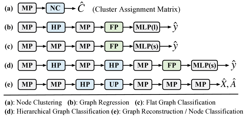
Figure 2: Illustration of model architectures for different tasks.

[b] Method Task Dataset Venue Code Link Flat Pooling Methods SortPool^{[1]$\spadesuit$$\clubsuit$} Graph Classification D&D, PROTEINS, NCI1, MUTAG, PTC, COLLAB, IMDB-B (M) AAAI’2018 https://shorturl.at/joAJ9 SOPool^[2] Graph Classification PROTEINS, NCI1, MUTAG, PTC, IMDB-B (M), COLLAB, RDT-B,RDT-M5K TPAMI’2020 – GMT^{[3]$\spadesuit$} Graph Classification D&D, PROTEINS, MUTAG, IMDB-B (M), COLLAB, HIV, TOX21, TOXC., BBBP ICLR’2021 https://shorturl.at/iorN3 Graph Reconstruction ZINC, Synthetic (Ring and Grid Graphs) Graph Generation QM9 DKEPool^[4] Graph Classification PROTEINS, NCI1, MUTAG, PTC, IMDB-B (M), HIV, BBBP TKDE’2022 https://shorturl.at/drz12 Node Clustering Pooling Methods DiffPool^{[5]$\spadesuit$$\clubsuit$} Graph Classification D&D, PROTEINS, ENZYMES, COLLAB, RDT-M12K NeurIPS’2018 https://shorturl.at/aflB3 MinCutPool^{[6]$\spadesuit$$\clubsuit$} Graph Classification D&D, PROTEINS, ENZYMES, IMDB-B (M), COLLAB ICML’2020 https://shorturl.at/zIOY9 Node Clustering Cora, Citeseer, Pubmed Graph Regression QM9 MemPool^[7] Graph Classification D&D, PROTEINS, ENZYMES, COLLAB, RDT-B ICLR’2020 https://shorturl.at/dqxY4 Graph Regression ESOL, Lipophilicity StructPool^[8] Graph Classification PROTEINS, ENZYMES,MUTAG, PTC, IMDB-B (M),COLLAB ICLR’2020 https://shorturl.at/fiJ01 HoscPool^[9] Graph Classification D&D, PROTEINS, NCI1, MUTAGEN., RDT-B, COX2-MD, ER-MD CIKM’2022 https://shorturl.at/abR26 Node Clustering Cora, Pubmed, CS, Photo, PC, Polblogs, Eu-email, Synthetic SEP^[10] Graph Classification D&D, PROTEINS, MUTAG, NCI1, IMDB-B (M), COLLAB ICML’2022 https://shorturl.at/ovDLT Graph Reconstruction Synthetic (Ring and Grid Graphs) Node Classification Cora, Citeseer, Pubmed Node Drop Pooling Methods  TopKPool^{[11]$\spadesuit$$\clubsuit$} Graph Classification D&D, PROTEINS, COLLAB ICML’2019 https://shorturl.at/cjlnr Node Classification Cora, Citeseer, Pubmed SAGPool^{[12]$\spadesuit$$\clubsuit$} Graph Classification D&D, PROTEINS, NCI1, NCI109, FRANK. ICML’2019 https://shorturl.at/bEJNQ ASAP^{[13]$\spadesuit$} Graph Classification D&D, PROTEINS, ENZYMES, NCI1, NCI109, MUTAGEN. AAAI’2020 https://shorturl.at/depuz VIPool^[14] Graph Classification D&D, PROTEINS, ENZYMES, IMDB-B (M), COLLAB NeurIPS’2020 https://shorturl.at/luvz1 Node Classification Cora, Citeseer, Pubmed GSAPool^[15] Graph Classification D&D, NCI1, NCI109, MUTAGEN. WWW’2020 https://shorturl.at/ciS02 PANPool^{[16]$\spadesuit$} Graph Classification PROTEINS, PROTEINS-FULL, NCI1, MUTAGEN., AIDS NeurIPS’2020 https://shorturl.at/OP015 TAPool^[17] Graph Classification D&D, PROTEINS, MUTAG, PTC TPAMI’2021 – IPool^[18] Graph Classification D&D, PROTEINS, ENZYMES, NCI1, NCI109, MNIST, CIFAR10 TNNLS’2021 – MVPool^[19] Graph Classification D&D, PROTEINS,ENZYMES, NCI1, NCI109, MUTAGEN. IMDB-B, RDT-M12K TKDE’2021 https://shorturl.at/fgqX1 Node Classification Cora, Citeseer, Pubmed, Coauthor-CS, Coauthor-Phy Node Clustering Cora, Citeseer, Pubmed Graph Clustering PROTEINS, NCI109, MUTAGEN. AdamGNN^[20] Graph Classification D&D, PROTEINS, MUTAG NCI1, NCI109, MUTAGEN. TKDE’2022 https://shorturl.at/tNQWZ Node Classification Cora, Citeseer, Pubmed, DBLP, ACM, Emails, Wiki, Ogbn-arxiv Link Prediction Cora, Citeseer, Pubmed, DBLP, ACM, Emails, Wiki

^[1]Zhang et al. (2018); ^[2]Wang and Ji (2020); ^[3]Baek et al. (2021); ^[4]Chen et al. (2022); ^[5]Ying et al. (2018); ^[6]Bianchi et al. (2020a); ^[7]Khasahmadi et al. (2020); ^[8]Yuan and Ji (2020); ^[9]Duval and Malliaros (2022); ^[10]Wu and others (2022); ^[11]Gao and Ji (2019); ^[12]Lee et al. (2019); ^[13]Ranjan et al. (2020); ^[14]Li et al. (2020b); ^[15]Zhang et al. (2020a); ^[16]Ma et al. (2020); ^[17]Gao et al. (2021a); ^[18]Gao et al. (2021b); ^[19]Zhang et al. (2021); ^[20]Zhong et al. (2022).

\raisebox{-0.9pt}{1}⃝ Models with $\spadesuit$ have another implementation by Pytorch available in Pytorch Geometric: https://pytorch-geometric.readthedocs.io/.

\raisebox{-0.9pt}{2}⃝ Models with $\clubsuit$ have another implementation by TensorFlow available in Spektral: https://graphneural.network/.

Table 4: A list of representative graph pooling methods.

4 Libraries for Graph Pooling

Benchmark Datasets.

Table 3 provides the statistics of commonly used datasets for evaluating graph pooling methods, which mainly come from two widely used repositories: TU dataset Morris et al. (2020), which contains over 130 datasets varying in content domains and dataset sizes, and Open Graph Benchmark (OGB) dataset Hu et al. (2020), which contains many large-scale benchmark datasets. The above datasets can be classified into four categories: 1) Social Networks. The social networks consider entities as nodes, and their social interactions as edges. 2) Protein Networks. The commonly used datasets include PROTEINS and D&D, where nodes correspond to amino acids, and edges are constructed if the distance between two nodes is below 6 Angstroms. 3) Molecule Graphs. The commonly used molecular datasets include NCI1 and MUTAG, in which nodes and edges refer to atoms and bonds, respectively. 4) Others. Besides the above three types of datasets, there are also some less commonly used datasets, such as synthetic datasets introduced by Knyazev et al. Knyazev et al. (2019), and image datasets Dwivedi et al. (2020), which are converted into graphs using super-pixels. The former is used to evaluate the generalization capability of pooling methods, and the latter is usually used to visualize the preserved information via graph pooling (usually used in node drop pooling methods), which helps analyze the interpretability of pooling methods.

Model Architectures.

The graph pooling methods are generally evaluated by two levels of graph tasks: 1) Node-level tasks include node classification and node clustering tasks, which are generally tested on a single graph in the form of transductive learning; 2) Graph-level tasks include graph classification, graph regression, graph reconstruction, and graph generation tasks, which are usually tested on multiple graphs in the form of inductive learning. Figure 2 summarizes the model architectures commonly used for various tasks. The abbreviations used in the figure are MP for message passing, NC for node clustering, HP for hierarchical pooling, FP for flat pooling, and UP for unpooling. In addition to the above task-oriented evaluations, Daniele et al. Grattarola et al. (2021) provided another two evaluation criteria, including preserving the information content of the node attributes and preserving the topological structure, which help to comprehensively quantify the ability of graph pooling.

Codes.

To facilitate the access to empirical analysis, we summarize the open-source codes of representative graph pooling studies in Table 4. Meanwhile, we list the applied tasks and corresponding benchmark datasets of each method. Due to space limitation, a more complete summary (over 150 papers reviewed) is presented in our GitHub repository . Moreover, we will update the repository in real-time as more methods and their implementations become available.

5 Applications

We briefly review the recent studies that incorporate the idea of graph pooling on a wide range of applications, which can be divided into two classes according to the type of datasets: 1) Structural datasets, where the data have explicit relational structures, such as molecular property prediction Wang et al. (2020); Khasahmadi et al. (2020), molecular generation Baek et al. (2021), protein-ligand binding affinity prediction Li et al. (2021b), 3D protein structure analysis Hermosilla et al. (2021), drug discovery Gaudelet et al. (2021), recommendation Wu et al. (2021); Chang et al. (2021); Liu et al. (2021b), community detection Liu et al. (2020), and relation extraction of knowledge graph Nadgeri et al. (2021). 2) Non-structural datasets, where the relational structures are implicit, and the graphs are built according to domain knowledge, such as cancer diagnosis Rhee et al. (2018); Adnan et al. (2020), brain data analysis Li et al. (2020c, 2021c); Kim et al. (2021); Pan et al. (2021); Demir et al. (2021); Gopinath et al. (2022), anti-spoofing and speech deepfaked detection Tak et al. (2021), natural language processing (NLP) Gao et al. (2019); Mao et al. (2022), computer vision (CV) Simonovsky and Komodakis (2017); Fey et al. (2018); Gu (2021), 3D point clouds Shen et al. (2018); Chen et al. (2020a); Wang et al. (2021), and multimodal sentiment analysis Mai et al. (2020).

The aforementioned studies have effectively decreased sample size Nadgeri et al. (2021) and incorporated hierarchical information Chen et al. (2020a) by utilizing either pre-existing or newly developed graph pooling techniques. This has resulted in notable enhancements across diverse applications, confirming the efficacy of graph pooling methods as demonstrated through experimental results in these works Wu et al. (2021); Pan et al. (2021); Shirian et al. (2022); Gopinath et al. (2022). Thus, the applicability of graph pooling has been established.

6 Challenges and Opportunities

6.1 Different Tasks and Multi-tasks

Challenge.

Table 4 demonstrates that most existing graph pooling methods focus on graph-level tasks, with few addressing node-level tasks like node classification. Graph pooling methods show promise in reducing the number of parameters, which can decrease time complexity and increase model resistance to over-fitting. Additionally, these methods have large receptive fields that capture high-order information. However, designing efficient and effective pooling/unpooling operators and integrating them into graph convolution networks for better performance in node-level tasks (e.g., node classification) are still key challenges.

Opportunity.

Some methods attempt to handle the node classification task with an encoder-decoder learning structure as shown in Figure 2 (e), where the unpooling operation is an important component. Several node drop pooling methods Li et al. (2020b); Zhang et al. (2021) utilize the unpooling operation proposed in the Graph U-net Gao and Ji (2019). Another important component is the convolution of decoder, termed deconvolution. Besides directly adopting the convolution of encoder as deconvolution, we can design a more reasonable deconvolution, inspired by DGN Li et al. (2021a), which reconstructs graph signals from smoothed node representations from the perspective of spectral domain. Therefore, future research directions include: 1) handling node-level tasks with an encoder-decoder structure by designing efficient unpooling and deconvolutional operators; 2) developing a unified graph pooling approach, through which node-level and graph-level tasks can be simultaneously handled Holtz et al. (2019); Zeng et al. (2021), which is beneficial since different tasks may benefit from each other.

6.2 Different Types of Graphs

Challenge.

The graph pooling methods discussed in Section 3 are primarily intended for plain graphs. However, there are also many other types of graphs in real-world datasets. Obviously, it is not optimal to directly apply the above existing graph pooling methods to these different types of graphs because they possess distinct characteristics. Therefore, there is a significant gap in the literature regarding the development of specific graph pooling operators tailored to handle diverse types of graphs.

Opportunity.

Recently, several graph pooling works have attempted to handle the rarely studied but commonly used graphs in real applications, such as heterogenous graphs Wu et al. (2021), spatio-temporal graphs Isufi and Mazzola (2021), and hypergraphs Jo et al. (2021). However, specific graph pooling operators for handling other types of graphs are still lacking. Therefore, we suggest two promising research opportunities: 1) extending the existing graph pooling methods or designing new pooling methods to deal with specific graphs in consideration of their properties, such as dynamic graphs, where graph structures and graph nodes dynamically change over time, directed graphs, where the edges have a direction, and signed networks, where signed edges represent positive or negative relationships between nodes; 2) devising a general pooling method, which can efficiently handle different types of graphs in a universal manner.

6.3 Interpretability

Challenge.

Although the existing graph pooling methods have achieved excellent results on various graph-based tasks, most of them show little interpretability Knyazev et al. (2019). This is particularly problematic for drug or disease-related problems where understanding the reasoning behind these methods is crucial. Although there has been some progress in interpreting node representation of GNNs Yuan et al. (2020), the interpretability of pooling methods remains largely unexplored.

Opportunity.

To exactly explain what has been learned from graph pooling operations, some studies Ying et al. (2018); Khasahmadi et al. (2020); Tang et al. (2021) have attempted to present the visualization of hierarchical clusters or hierarchical community structures captured by pooling operations, but they do not provide quantitative analyses to assess the quality of clustering. Moreover, the interpretability of pooling operations is still not well explored. Therefore, there is a need for further research in this area. A promising direction would be to extend existing studies on interpreting GNNs Yuan et al. (2020) to include graph pooling.

6.4 Robustness

Challenge.

Since many applications of graph pooling methods are risk-sensitive, e.g., drug design and disease diagnosis, the robustness of methods is essential and indispensable for actual usages. However, according to the analysis in recent studies Tang et al. (2020); Roy et al. (2021); Liu et al. (2022a), most graph pooling methods fail to distinguish the noise information from the input graph, thus dramatically degrading their performance when the input graph is perturbed in terms of features or topology.

Opportunity.

Although some initial studies have been conducted on the robustness of graph machine learning, few studies have explored the robustness of graph pooling methods. So far, only an adversarial attack framework has been proposed by Tang et al. Tang et al. (2020) to evaluate the robustness of graph pooling methods. Therefore, there is much work to be done to develop a robust graph pooling method for practical applications, such as: 1) building up a comprehensive adversarial attack framework encompasses various types of attacks; 2) designing adversarial defense graph pooling methods. One potential solution is to extend the techniques used for enhancing the robustness of graph machine learning into improving the robustness of graph pooling methods.

6.5 Large-scale Data

Challenge.

Most graph pooling methods are tested on small benchmark datasets, which may be insufficient for comparisons among different graph pooling models. For example, applying graph pooling methods to small node classification datasets, i.e., Cora, is insufficient to assess their effectiveness in reducing the time and space complexity. Only a few works have attempted to deal with relatively larger graph datasets Zhong et al. (2022). Additionally, the efficiency of pooling methods is crucial. The high cost of time or space limits their applicability to large-scale datasets. Node clustering pooling methods, for example, suffer from high storage complexities due to the computation of dense assignment matrices Grattarola et al. (2021).

Opportunity.

Hence, we suggest the following research objectives: 1) performing further verifications on large-scale graph datasets, e.g., on the Open Graph Benchmark Hu et al. (2020), which is a recently proposed large-scale graph machine learning benchmark; 2) designing more efficient graph pooling methods and making them more practical with constrained resource in real-world scenarios.

6.6 Expressive Power

Challenge.

Most existing graph pooling methods are designed by intuition, and their performance gains are evaluated by empirical experiments. The lack of the means by which we can characterize the expressive power of graph pooling operators hinders the creation of more powerful graph pooling models Xu et al. (2019).

Opportunity.

Only a limited number of studies Murphy et al. (2019); Chen et al. (2020b); Baek et al. (2021) have examined the expressive ability of their models in terms of the 1-Weisfeiler-Lehman (WL) test. Recently, Bianchi et al. Bianchi and Lachi (2023) conducted an comprehensive analysis on the expressive power of graph pooling techniques. Therefore, based on their theoretical findings, it is promising and significant to explore more powerful graph pooling methods as future research directions.

6.7 Generalize to Out-of-Distribution Data.

Challenge.

Graph Neural Networks are proposed without considering the agnostic distribution shifts between training graphs and testing graphs, causing the degeneration of the generalization ability in out-of-distribution (OOD) settings. Boris et al. Knyazev et al. (2019) have attempted to improve the generalization ability of GNNs with the help of graph pooling models. Moreover, Xu et al. Xu et al. (2021) emphasized the significance of selecting appropriate pooling functions for enabling GNNs to generalize over graph data beyond the distribution of training data.

Opportunity.

Recently, to improve the OOD generalization ability of GNNs has become an appealing and non-trivial task. According to the above introduction, utilizing graph pooling techniques can be an effective approach to improve the generalization capability of GNNs on OOD graph data.

References

- Adnan et al. (2020) Mohammed Adnan, et al. Representation learning of histopathology images using graph neural networks. In CVPR Workshop, 2020.
- Atwood and Towsley (2016) James Atwood et al. Diffusion-convolutional neural networks. In NeurIPS, 2016.
- Bacciu and Sotto (2019) Davide Bacciu et al. A non-negative factorization approach to node pooling in graph convolutional neural networks. In AIIA, 2019.
- Baek et al. (2021) Jinheon Baek, et al. Accurate learning of graph representations with graph multiset pooling. In ICLR, 2021.
- Bai et al. (2019) Yunsheng Bai, et al. Unsupervised inductive graph-level representation learning via graph-graph proximity. In IJCAI, 2019.
- Bai et al. (2021) Lu Bai, et al. Learning graph convolutional networks based on quantum vertex information propagation. IEEE TKDE, 2021.
- Bianchi and Lachi (2023) Filippo Maria Bianchi et al. The expressive power of pooling in graph neural networks. arXiv:2304.01575, 2023.
- Bianchi et al. (2020a) Filippo Maria Bianchi, et al. Spectral clustering with graph neural networks for graph pooling. In ICML, 2020.
- Bianchi et al. (2020b) Filippo Maria Bianchi, et al. Hierarchical representation learning in graph neural networks with node decimation pooling. IEEE TNNLS, 2020.
- Bodnar et al. (2020) Cristian Bodnar, et al. Deep graph mapper: Seeing graphs through the neural lens. In NeurIPS Workshop, 2020.
- Cangea et al. (2018) Cătălina Cangea, et al. Towards sparse hierarchical graph classifiers. arXiv:1811.01287, 2018.
- Chang et al. (2021) Jianxin Chang, et al. Sequential recommendation with graph neural networks. In SIGIR, 2021.
- Chen et al. (2019) Ting Chen, et al. Are powerful graph neural nets necessary? a dissection on graph classification. arXiv:1905.04579, 2019.
- Chen et al. (2020a) Chaofan Chen, et al. Hapgn: Hierarchical attentive pooling graph network for point cloud segmentation. IEEE TMM, 2020.
- Chen et al. (2020b) Zhengdao Chen, et al. Can graph neural networks count substructures? In NeurIPS, 2020.
- Chen et al. (2022) Kaixuan Chen, et al. Distribution knowledge embedding for graph pooling. IEEE TKDE, 2022.
- Demir et al. (2021) Andac Demir, et al. Eeg-gnn: Graph neural networks for classification of electroencephalogram (eeg) signals. arXiv:2106.09135, 2021.
- Diehl (2019) Frederik Diehl. Edge contraction pooling for graph neural networks. arXiv:1905.10990, 2019.
- Du et al. (2021) Jinlong Du, et al. Multi-channel pooling graph neural networks. In IJCAI, 2021.
- Duval and Malliaros (2022) Alexandre Duval et al. Higher-order clustering and pooling for graph neural networks. In CIKM, 2022.
- Duvenaud et al. (2015) David Duvenaud, et al. Convolutional networks on graphs for learning molecular fingerprints. In NeurIPS, 2015.
- Dwivedi et al. (2020) Vijay Prakash Dwivedi, et al. Benchmarking graph neural networks. arXiv:2003.00982, 2020.
- Errica et al. (2020) Federico Errica, et al. A fair comparison of graph neural networks for graph classification. In ICLR, 2020.
- Fan et al. (2020) Xiaolong Fan, et al. Structured self-attention architecture for graph-level representation learning. Pattern Recognition, 2020.
- Fey et al. (2018) Matthias Fey, et al. Splinecnn: Fast geometric deep learning with continuous b-spline kernels. In CVPR, 2018.
- Gao and Ji (2019) Hongyang Gao et al. Graph u-nets. In ICML, 2019.
- Gao et al. (2019) Hongyang Gao, et al. Learning graph pooling and hybrid convolutional operations for text representations. In WWW, 2019.
- Gao et al. (2020) Zhangyang Gao, et al. Lookhops: light multi-order convolution and pooling for graph classification. arXiv:2012.15741, 2020.
- Gao et al. (2021a) H. Gao, et al. Topology-aware graph pooling networks. IEEE TPAMI, 2021.
- Gao et al. (2021b) Xing Gao, et al. ipool–information-based pooling in hierarchical graph neural networks. IEEE TNNLS, 2021.
- Gaudelet et al. (2021) Thomas Gaudelet, et al. Utilizing graph machine learning within drug discovery and development. Briefings in Bioinformatics, 2021.
- Gopinath et al. (2022) Karthik Gopinath, et al. Learnable pooling in graph convolutional networks for brain surface analysis. IEEE TPAMI, 2022.
- Grattarola et al. (2021) Daniele Grattarola, et al. Understanding pooling in graph neural networks. arXiv:2110.05292, 2021.
- Gu (2021) Jindong Gu. Interpretable graph capsule networks for object recognition. AAAI, 2021.
- Hermosilla et al. (2021) Pedro Hermosilla, et al. Intrinsic-extrinsic convolution and pooling for learning on 3d protein structures. In ICLR, 2021.
- Holtz et al. (2019) Chester Holtz, et al. Multi-task learning on graphs with node and graph level labels. In NeurIPS Workshop, 2019.
- Hu et al. (2020) Weihua Hu, et al. Open graph benchmark: Datasets for machine learning on graphs. arXiv:2005.00687, 2020.
- Huang et al. (2019) Jingjia Huang, et al. Attpool: Towards hierarchical feature representation in graph convolutional networks via attention mechanism. In ICCV, 2019.
- Isufi and Mazzola (2021) Elvin Isufi et al. Graph-time convolutional neural networks. arXiv:2103.01730, 2021.
- Itoh et al. (2022) Takeshi D. Itoh, et al. Multi-level attention pooling for graph neural networks: Unifying graph representations with multiple localities. Neural Networks, 2022.
- Jo et al. (2021) Jaehyeong Jo, et al. Edge representation learning with hypergraphs. In NeurIPS, 2021.
- Khasahmadi et al. (2020) Amir Hosein Khasahmadi, et al. Memory-based graph networks. In ICLR, 2020.
- Kim et al. (2021) Byung-Hoon Kim, et al. Learning dynamic graph representation of brain connectome with spatio-temporal attention. In NeurIPS, 2021.
- Kipf and Welling (2017) Thomas N. Kipf et al. Semi-supervised classification with graph convolutional networks. In ICLR, 2017.
- Knyazev et al. (2019) Boris Knyazev, et al. Understanding attention and generalization in graph neural networks. In NeurIPS, 2019.
- Lee et al. (2019) Junhyun Lee, et al. Self-attention graph pooling. In ICML, 2019.
- Lee et al. (2021) Dongha Lee, et al. Learnable structural semantic readout for graph classification. In ICDM, 2021.
- Li et al. (2016) Yujia Li, et al. Gated graph sequence neural networks. In ICLR, 2016.
- Li et al. (2020a) Juanhui Li, et al. Graph pooling with representativeness. In ICDM, 2020.
- Li et al. (2020b) Maosen Li, et al. Graph cross networks with vertex infomax pooling. In NeurIPS, 2020.
- Li et al. (2020c) Xiaoxiao Li, et al. Pooling regularized graph neural network for fmri biomarker analysis. In MICCAI, 2020.
- Li et al. (2021a) Jia Li, et al. Deconvolutional networks on graph data. NeurIPS, 2021.
- Li et al. (2021b) Shuangli Li, et al. Structure-aware interactive graph neural networks for the prediction of protein-ligand binding affinity. In KDD, 2021.
- Li et al. (2021c) Xiaoxiao Li, et al. Braingnn: Interpretable brain graph neural network for fmri analysis. Medical Image Analysis, 2021.
- Liang et al. (2020) Yanyan Liang, et al. Mxpool: Multiplex pooling for hierarchical graph representation learning. arXiv:2004.06846, 2020.
- Liu et al. (2020) Fanzhen Liu, et al. Deep learning for community detection: progress, challenges and opportunities. In IJCAI, 2020.
- Liu et al. (2021a) Ning Liu, et al. Hierarchical adaptive pooling by capturing high-order dependency for graph representation learning. IEEE TKDE, 2021.
- Liu et al. (2021b) Y. Liu, et al. Learning hierarchical review graph representations for recommendation. IEEE TKDE, 2021.
- Liu et al. (2022a) Chuang Liu, et al. On exploring node-feature and graph-structure diversities for node drop graph pooling, 2022.
- Liu et al. (2022b) Ning Liu, et al. Unsupervised hierarchical graph pooling via substructure-sensitive mutual information maximization. In CIKM, 2022.
- Liu et al. (2023) Chuang Liu, et al. Masked graph auto-encoder constrained graph pooling. In ECML-PKDD, 2023.
- Ma et al. (2019) Yao Ma, et al. Graph convolutional networks with eigenpooling. In KDD, 2019.
- Ma et al. (2020) Zheng Ma, et al. Path integral based convolution and pooling for graph neural networks. In NeurIPS, 2020.
- Ma et al. (2021) Xiaoxiao Ma, et al. A comprehensive survey on graph anomaly detection with deep learning. IEEE TKDE, 2021.
- Mai et al. (2020) Sijie Mai, et al. Analyzing unaligned multimodal sequence via graph convolution and graph pooling fusion. arXiv:2011.13572, 2020.
- Mao et al. (2022) Qianren Mao, et al. Higil: Hierarchical graph inference learning for fact checking. In ICDM, 2022.
- Mesquita et al. (2020) Diego Mesquita, et al. Rethinking pooling in graph neural networks. In NeurIPS, 2020.
- Morris et al. (2020) Christopher Morris, et al. Tudataset: A collection of benchmark datasets for learning with graphs. arXiv:2007.08663, 2020.
- Murphy et al. (2019) Ryan Murphy, et al. Relational pooling for graph representations. In ICML, 2019.
- Nadgeri et al. (2021) Abhishek Nadgeri, et al. KGPool: Dynamic knowledge graph context selection for relation extraction. In ACL, 2021.
- Navarin et al. (2019) Nicolò Navarin, et al. Universal readout for graph convolutional neural networks. In IJCNN, 2019.
- Noutahi et al. (2019) Emmanuel Noutahi, et al. Towards interpretable sparse graph representation learning with laplacian pooling. arXiv:1905.11577, 2019.
- Pan et al. (2021) Li Pan, et al. Identifying autism spectrum disorder based on individual-aware down-sampling and multi-modal learning. arXiv:2109.09129, 2021.
- Pang et al. (2021) Yunsheng Pang, et al. Graph pooling via coarsened graph infomax. In SIGIR, 2021.
- Papp et al. (2021) Pál András Papp, et al. Dropgnn: Random dropouts increase the expressiveness of graph neural networks. NeurIPS, 2021.
- Qin et al. (2020) Jian Qin, et al. Uniform pooling for graph networks. Appl. Sci., 2020.
- Ranjan et al. (2020) Ekagra Ranjan, et al. Asap: Adaptive structure aware pooling for learning hierarchical graph representations. In AAAI, 2020.
- Rhee et al. (2018) Sungmin Rhee, et al. Hybrid approach of relation network and localized graph convolutional filtering for breast cancer subtype classification. In IJCAI, 2018.
- Roy et al. (2021) Kashob Kumar Roy, et al. Structure-aware hierarchical graph pooling using information bottleneck. In IJCNN, 2021.
- Shen et al. (2018) Y. Shen, et al. Mining point cloud local structures by kernel correlation and graph pooling. In CVPR, 2018.
- Shirian et al. (2022) Amir Shirian, et al. Dynamic emotion modeling with learnable graphs and graph inception network. IEEE TMM, 2022.
- Simonovsky and Komodakis (2017) Martin Simonovsky et al. Dynamic edge-conditioned filters in convolutional neural networks on graphs. In CVPR, 2017.
- Su et al. (2021) Zidong Su, et al. Hierarchical graph representation learning with local capsule pooling. In MMAsia, 2021.
- Tak et al. (2021) Hemlata Tak, et al. End-to-end spectro-temporal graph attention networks for speaker verification anti-spoofing and speech deepfake detection. arXiv:2107.12710, 2021.
- Tang et al. (2020) Haoteng Tang, et al. Adversarial attack on hierarchical graph pooling neural networks. arXiv:2005.11560, 2020.
- Tang et al. (2021) Haoteng Tang, et al. Commpool: An interpretable graph pooling framework for hierarchical graph representation learning. Neural Networks, 2021.
- Vinyals et al. (2016) Oriol Vinyals, et al. Order matters: Sequence to sequence for sets. In ICLR, 2016.
- Wang and Ji (2020) Zhengyang Wang et al. Second-order pooling for graph neural networks. IEEE TPAMI, 2020.
- Wang et al. (2020) Yu Guang Wang, et al. Haar graph pooling. In ICML, 2020.
- Wang et al. (2021) Jie Wang, et al. Papooling: Graph-based position adaptive aggregation of local geometry in point clouds. arXiv:2111.14067, 2021.
- Wei et al. (2021) Lanning Wei, et al. Pooling architecture search for graph classification. In CIKM, 2021.
- Wu and others (2022) Junran Wu et al. Structural entropy guided graph hierarchical pooling. In ICML, 2022.
- Wu et al. (2019) Jun Wu, et al. Demo-net: Degree-specific graph neural networks for node and graph classification. In KDD, 2019.
- Wu et al. (2021) Chuhan Wu, et al. User-as-graph: User modeling with heterogeneous graph pooling for news recommendation. In IJCAI, 2021.
- Xu et al. (2019) Keyulu Xu, et al. How powerful are graph neural networks? In ICLR, 2019.
- Xu et al. (2021) Keyulu Xu, et al. How neural networks extrapolate: From feedforward to graph neural networks. In ICLR, 2021.
- Yang et al. (2021) Jinyu Yang, et al. Hierarchical graph capsule network. In AAAI, 2021.
- Ying et al. (2018) Zhitao Ying, et al. Hierarchical graph representation learning with differentiable pooling. In NeurIPS, 2018.
- Yuan and Ji (2020) Hao Yuan et al. Structpool: Structured graph pooling via conditional random fields. In ICLR, 2020.
- Yuan et al. (2020) Hao Yuan, et al. Explainability in graph neural networks: A taxonomic survey. arXiv:2012.15445, 2020.
- Zeng et al. (2021) Hanqing Zeng, et al. Decoupling the depth and scope of graph neural networks. In NeurIPS, 2021.
- Zhang et al. (2018) Muhan Zhang, et al. An end-to-end deep learning architecture for graph classification. In AAAI, 2018.
- Zhang et al. (2020a) Liang Zhang, et al. Structure-feature based graph self-adaptive pooling. In WWW, 2020.
- Zhang et al. (2020b) Zhen Zhang, et al. Hierarchical graph pooling with structure learning. In AAAI, 2020.
- Zhang et al. (2021) Zhen Zhang, et al. Hierarchical multi-view graph pooling with structure learning. IEEE TKDE, 2021.
- Zhong et al. (2022) Zhiqiang Zhong, et al. Multi-grained semantics-aware graph neural networks. IEEE TKDE, 2022.
- Zhou et al. (2020) Kaixiong Zhou, et al. Multi-channel graph neural networks. In IJCAI, 2020.