A review of path following control strategies for autonomous robotic vehicles: theory, simulations, and experiments

Abstract

This article presents an in-depth review of the topic of path following for autonomous robotic vehicles, with a specific focus on vehicle motion in two dimensional space (2D). From a control system standpoint, path following can be formulated as the problem of stabilizing a path following error system that describes the dynamics of position and possibly orientation errors of a vehicle with respect to a path, with the errors defined in an appropriate reference frame. In spite of the large variety of path following methods described in the literature we show that, in principle, most of them can be categorized in two groups: stabilization of the path following error system expressed either in the vehicle’s body frame or in a frame attached to a “reference point” moving along the path, such as a Frenet–Serret (F-S) frame or a Parallel Transport (P-T) frame. With this observation, we provide a unified formulation that is simple but general enough to cover many methods available in the literature. We then discuss the advantages and disadvantages of each method, comparing them from the design and implementation standpoint. We further show experimental results of the path following methods obtained from field trials testing with under-actuated and fully-actuated autonomous marine vehicles. In addition, we introduce open-source Matlab and Gazebo/ROS simulation toolboxes that are helpful in testing path following methods prior to their integration in the combined guidance, navigation, and control systems of autonomous vehicles.

1 Introduction

Path-following (PF) is one of the most fundamental tasks to be executed by autonomous vehicles. It consists of driving a vehicle to and maintaining it on a pre-defined path while tracking a path-dependent speed profile. Unlike trajectory tracking, the path is not parameterized by time but rather by any other useful parameter that in some cases may be the path length. Thus, there is more flexibility in making the vehicle first converge to the path smoothly then move along it while tracking a given speed assignment. Path following is useful in many applications where the main objective is to accurately traverse the path, while maintaining a certain speed is a secondary task. Stated in simple terms, it is not required for the vehicle to be at specific positions at specific instants of time, a strong requirement in trajectory tracking. All that is required is for the vehicle to go through specific points in space while trying to meet speed assignments, but absolute time is not of overriding importance. From a technical standpoint, when compared with trajectory tracking, path following has the potential to exhibit smoother convergence properties and reduced actuator activity [AH07]. For these reasons, in a vast number of applications path-following is performed by a variety of heterogeneous vehicles, of which marine vehicles [RHJ⁺19, Fos11, NMM20], ground vehicles such as Mars rovers [HCC⁺04, FBT97, KZ09], fixed wing aerial vehicles [NBMB07, PDH07, SSS14], autonomous cars [GCC⁺19, S⁺09, DLOS98, RMNM21], and quad-rotors [RPM19] are representative examples.
The task of deriving control strategies to solve the PF problem is technically challenging, specially in the presence of non-holonomic constraints, and often involves the use of a nonlinear control techniques such as backstepping [EP00, LSP06], feedback linearization [AWN12], sliding mode control [DOO03], vector field [NBMB07, WC19], linear model predictive control (MPC) [RGNR⁺09, KZ09], and nonlinear MPC (NMPC) [HPJ20, AAJ13, GCC⁺19, SSNS18]. Other path following algorithms exploit learning-based methods such as Learning-based MPC (LB-MPC) [OSBC16, RMNM20], reinforcement learning-based control [ML18, KZL19, WDWR21], among others. Due to the proliferation of robotic vehicles and their applications, the past decades have witnessed the development of a multitude of path-following methods. Therefore, in order to provide a critical assessment of the collective work done, this paper contains a comprehensive survey, aimed at comparing different PF methods from the design and implementation standpoint and discussing the advantages and disadvantages of each method. In particular, we show that an important classification of path-following algorithms is given by the choice of reference frame in which the path-following error is defined. In general, the latter is defined either in the vehicle’s body frame or in a frame attached to a “reference point” moving along the path such as the Frenet–Serret (F-S) frame or the Parallel Transport (P-T) frame.
In the literature, one can find other survey papers of path following methods such as [SSS14] for fixed-wing aerial vehicles, [RPM19] for quadrotors, or autonomous car-like robot [RMNM21]. However, the aforementioned survey papers do not describe in detail the theory that supports the methods described and, while they contain simulation results, they do not present a comparison of the performance of the methods in field tests with real vehicles. Moreover, the above surveys focus on specific types of autonomous vehicles, and do not consider some of the unique characteristics of under-actuated marine vehicles such as non-holonomic constraints in [RPM19] or the requirement that a vehicle track a desired speed profile along the path [SSS14, RMNM21]. In the current review paper, instead of focusing on a particular type of vehicle, we emphasize the common principle underlying path following methods, that can be applied and extended to a large class of vehicles, the simplified motion of which can be described by the same class of kinematic models. Furthermore, the present paper also provides a rigorous theoretical proof of the methods reviewed that is absent in the previous surveys. We introduce simulation toolboxes written in Matlab and ROS/Gazebo that are helpful in testing the path following methods and integrating them in guidance, navigation, and control systems. To conclude, we report experimental results with a Medusa class autonomous marine vehicles [ABG⁺16] that have been widely used in EU projects such as WiMust [AMP⁺16] and MORPH [CBB⁺15]. In short, the main contributions of this paper include

1. An in-depth review of standard path-following methods in two dimensional space (2D) explaining in detail the theoretical principles of the different methods.

2. A discussion of the advantages and disadvantages of each method, comparing them from the design and implementation standpoint.

3. A Matlab simulation toolbox and ROS/Gazebo simulation packages of path-following methods.

4. A description of experimental results of field trials at sea with the Medusa under-actuated and fully-actuated robotic vehicles, followed by an assessment of the performance obtained in real-life situations.

The paper is organized as follows. The path following problem is formulated in Section 2. Section 3 describes path following methods for under-actuated vehicles. Section 4 extends the path following methods to the case where external unknown disturbances occur. Section 5 reviews a path following method developed for fully-actuated vehicles with arbitrary heading. The implementation in Matlab and Gazebo/ROS simulation toolboxes for testing path following methods are introduced in Section 6. Experimental results with autonomous marine vehicles are presented in Section 7. Section 8 provides a discussion on advantages and disadvantages of the path following methods and practical issues when the vehicles dynamics are taken into account. Finally, Section 9 contains the main conclusions.

2 Problem formulation and common principles of path following methods

2.1 Vehicle kinematic models

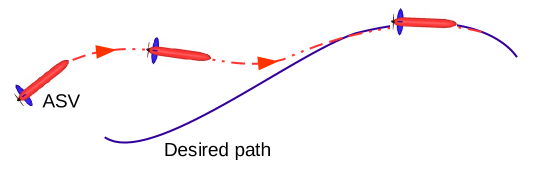
Figure 2.1: Geometric illustration of the path following problem.

Path following refers to the problem of making a vehicle converge to and follow a spatial path while asymptotically tracking a desired speed profile along the path; see Fig. 2.1 that shows an ASV executing a path following maneuver. From a control system standpoint, the structure of a complete path following system is captured in Fig. 2.2(a). In this architecture, the outer-loop path following controller implements a guidance strategy, in charge of computing desired references (e.g. linear and angular speeds, or orientations) to steer the vehicle along the path with a desired speed profile $U_{d}$. These references act as inputs to autopilots that play the role of inner-loop controllers, in charge of generating suitable forces and torque for the vehicle in order to track the desired references, thus achieving the path following objectives.
In practice, to simplify the design of a path following controller, it is commonly assumed that the responses the inner-loops are sufficiently fast so that the influence of the latter in the complete system can be neglected. Under these ideal conditions, the path following control system can be simplified by considering the kinematics model only, as shown in Fig. 2.2(b). Our purpose in the present paper is to review the core ideas behind existing path following methods in the literature, therefore we primarily focus on those designed for the vehicle kinematics only. We then treat the effect of the inner-loops as an internal disturbances and analyze the robustness of the path following methods under these disturbances accordingly.

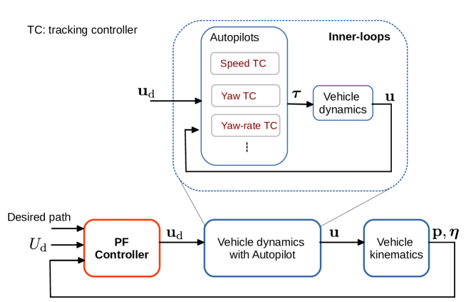
a) A complete path following control system  
 

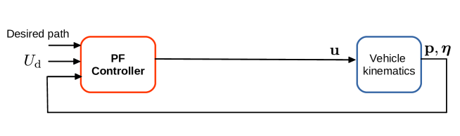
b) A simplified path following system for PF controller design

Figure 2.2: Path following control systems; ${\bf u}_{\rm d}$: reference inputs (e.g. desired linear and angular speeds, orientations) for the autopilots; ${\bf p}$ and $\boldsymbol{\eta}$: the vehicle’s position and orientation, respectively, ${\boldsymbol{\tau}}$: force and torque, $U_{\rm d}$: desired speed profile that the vehicle must track.

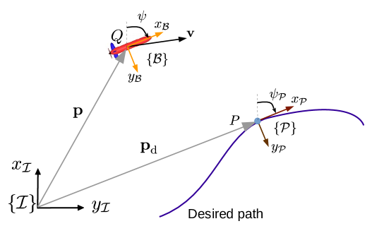
Figure 2.3: Geometric illustration of the path following problem. $\{I\},\{\mathcal{B}\}$, and $\{\mathcal{P}\}$ denote inertial/global, the vehicle body, and path frames, respectively. The symbols ${\bf p}$ and ${\bf p}_{\rm d}$ represent the position vectors of the vehicle and a generic point on the path, respectively expressed in $\{\mathcal{I}\}$.

The vehicle kinematic models that will be used to derive path following control laws in the present paper will be described next. The vehicle’s motion with respect to a path is illustrated Fig.2.3. The following notation and nomenclature will be used. The symbol $\{\mathcal{I}\}=\{x_{\mathcal{I}},y_{\mathcal{I}}\}$ denotes an inertial (global) North-East (NE) frame, where the axis $x_{\mathcal{I}}$ points to the North and the axis $y_{\mathcal{I}}$ points to the East. Let $Q$ be the center of mass of the vehicle and denote by ${\bf p}=[x,y]^{\top}\in\mathbb{R}^{2}$ the position of $Q$ in $\left\{\mathcal{I}\right\}$. Let also $\{\mathcal{B}\}=\{x_{\mathcal{B}},y_{\mathcal{B}}\}$ be a body-fixed frame whose origin is located at $Q$. In addition, denote by ${\bf v}=[u,v]^{\top}\in\mathbb{R}^{2}$ the vehicle’s velocity vector with respect to the fluid, measured in $\left\{\mathcal{B}\right\}$, where $u,v$ are the surge/longitudinal and sway/lateral speeds, respectively. With the above notation, the “general” 3-DOF vehicle’s kinematic model is described by

$$\begin{split}\dot{x}&=u\cos(\psi)-v\sin(\psi)+v_{\rm{cx}}\\ \dot{y}&=u\sin(\psi)+v\cos(\psi)+v_{\rm{cy}}\\ \dot{\psi}&=r,\end{split}$$ (1)

where $\psi$ is the vehicle’s heading/yaw angle and $r$ is its heading/yaw rate, $v_{\rm cx}$ and $v_{\rm cy}$ are components of vector ${\bf v}_{c}=[v_{\rm cx},v_{\rm cy}]^{\top}\in\mathbb{R}^{2}$ that represents the effect of external unknown disturbances (e.g. ocean current in the case of marine vehicles and wind in the case of aerial vehicles) in $\left\{\mathcal{I}\right\}$. For the sake of clarity, in the present paper we consider the following three separate subcases of (1).

2.1.1 Scenario 1: under-actuated vehicle without external disturbances

In this scenario we assume that the vehicle is under-actuated and that the vehicle’s lateral motion and external disturbances are so small so that they can be neglected, that is, making $v,v_{\rm cx},v_{\rm cy}$ zero we obtain

$$\begin{split}\dot{x}&=u\cos(\psi)\\ \dot{y}&=u\sin(\psi)\\ \dot{\psi}&=r.\end{split}$$ (2)

We also assume that the longitudinal speed ($u$) and the heading ($\psi$) or heading rate ($r$) can be tracked with good accuracy by inner-loop controllers. Although (2) is a significant simplification of (1) it still captures sufficiently well the behavior of a large class of under-actuated vehicles, including unicycle mobile robots [MS93, YP17], fixed-wing UAVs undergoing planar motion [NBMB07, ZWCW20, LMC13, YLC⁺21, RAF⁺15], and a wide class of under-actuated autonomous marine vehicles (AMVs). The later include the Medusa and Delfim [ABG⁺16] and Charlie [BBCL09] vehicles, for which the sway speed is in practice so small that it can be neglected. Snapshots of several vehicles mentioned above are shown in Fig.2.4. In the literature, most path following methods are proposed for the kinematic model (2); in accordance, a large part of this paper presented in Section 3 is devoted to their review.

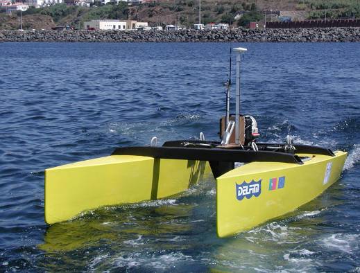
a) Under-actuated Medusa [ABG⁺16]              b) Delfim [AOO⁺06]
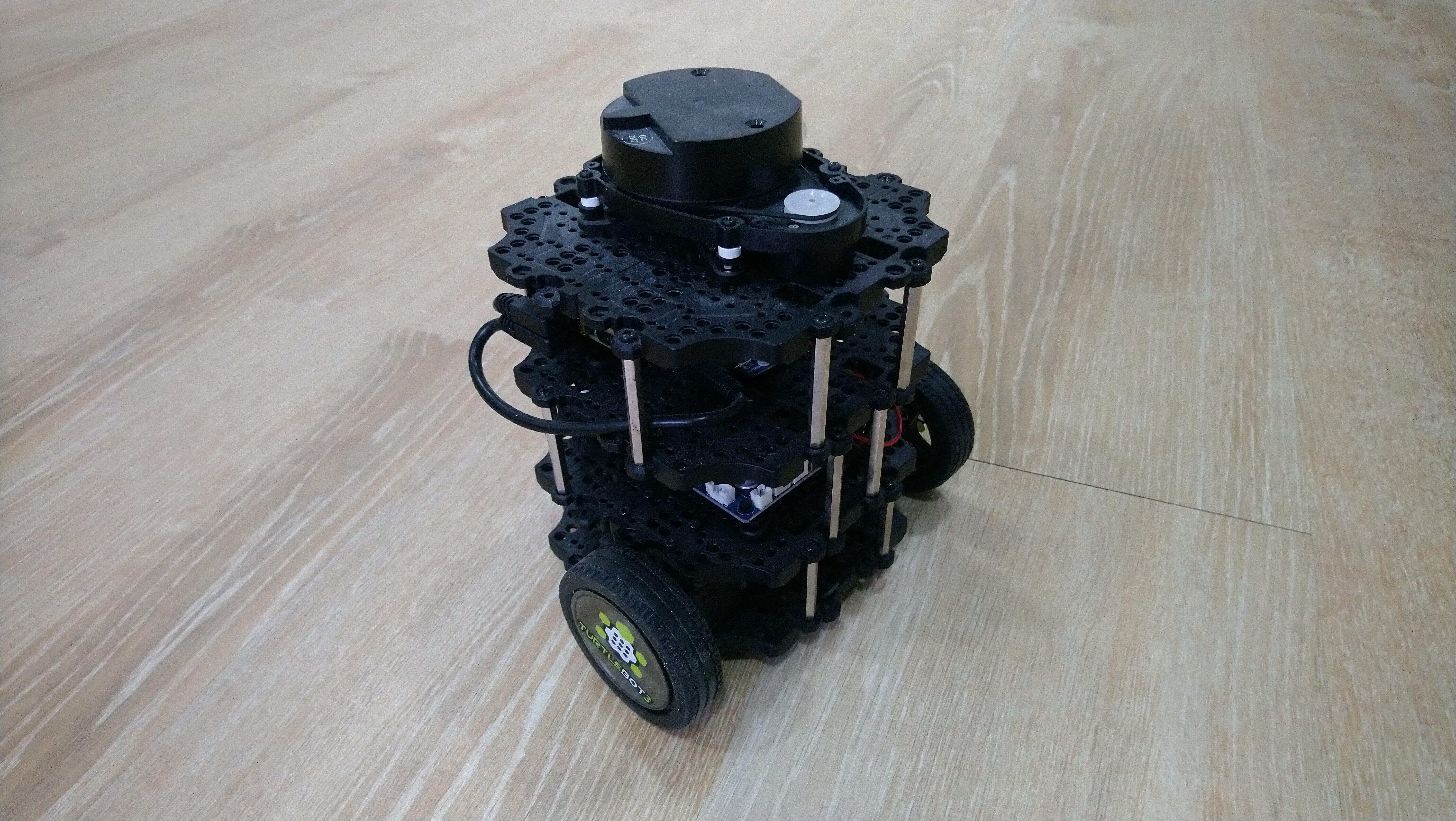
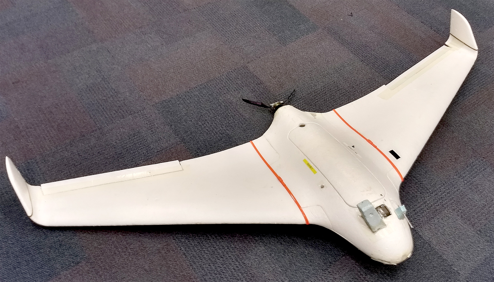
c) Turtlebot Burger [YP17]                       d) X8 fixed-wing UAV [YLC⁺21]

Figure 2.4: Under-actuated robotic vehicles

2.1.2 Scenario 2: under-actuated vehicle with external disturbances

In this scenario the vehicle motion is influenced significantly by external disturbances that can not be neglected; however, the lateral sway is still small enough to be ignored (i.e. $v=0$). Given these assumptions, the vehicle kinematics model is given by

$$\begin{split}\dot{x}&=u\cos(\psi)+v_{cx}\\ \dot{y}&=u\sin(\psi)+v_{cy}\\ \dot{\psi}&=r.\end{split}$$ (3)

Note also that similar to Scenario 1, the vehicle is under-actuated. Path following methods developed for this model will be discussed in Section 4.

2.1.3 Scenario 3: fully or over-actuated vehicle

In this scenario we assume that the lateral speed is significant and can not be neglected. However, for simplicity we neglect the effect of external disturbances. With these assumptions, the vehicle kinematic model is given by

$$\begin{split}\dot{x}&=u\cos(\psi)-v\sin(\psi)\\ \dot{y}&=u\sin(\psi)+v\cos(\psi)\\ \dot{\psi}&=r.\end{split}$$ (4)

In this scenario we assume further that the vehicle is fully or over-actuated in that its longitudinal and lateral speeds and heading rate can be controlled simultaneously. Fig.2.5 shows snapshots of several fully-actuated vehicles that meet these assumptions. For this scenario we are interested the path following problem in which the vehicle is not only required to follow a predefined path but also to maneuver such that its heading tracks an arbitrary heading reference. This scenario will be presented in Section 5.

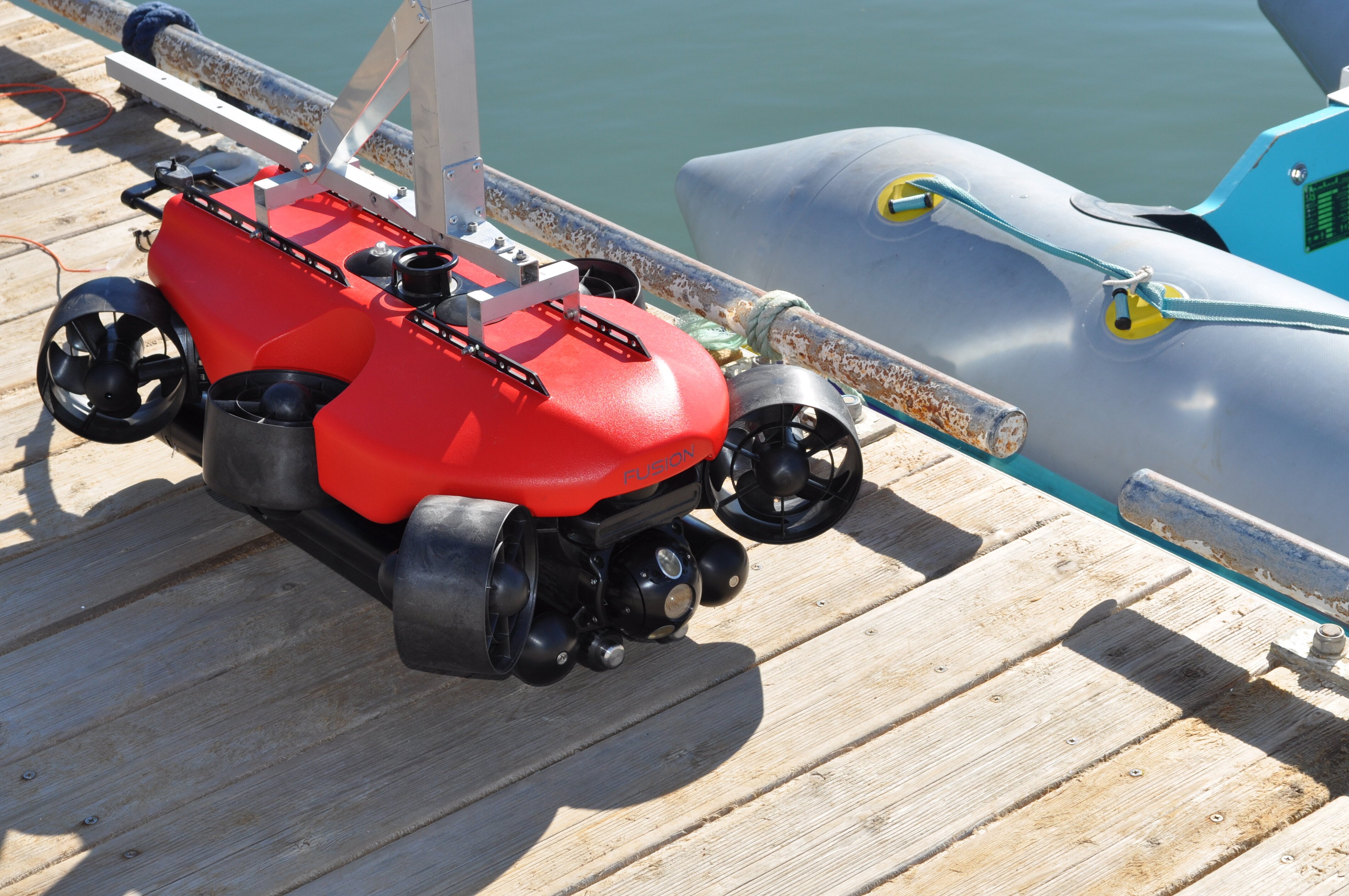
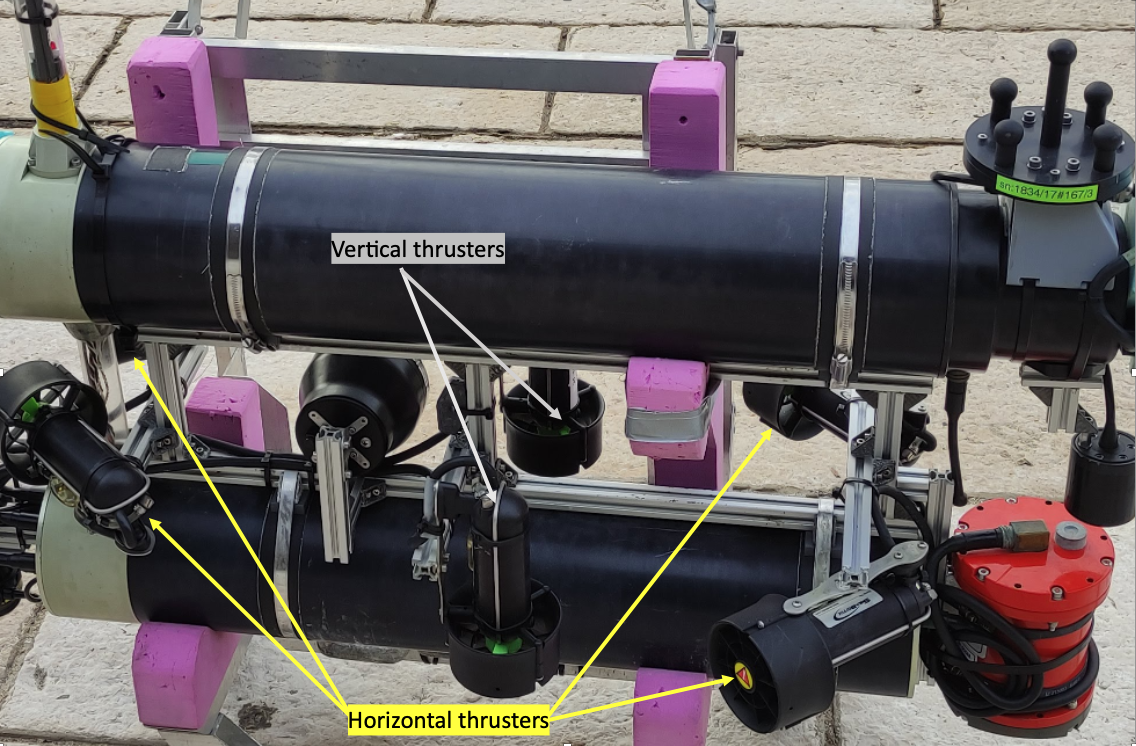
Figure 2.5: Over-actuated robotic vehicles. Left: Fusion vehicle, produced by Strategic Robot Systems company equipped with the Guidance, Navigation, and Control systems developed by IST Lisbon; Right: M-Vector vehicle, developed by IST Lisbon. Notice in both vehicles the existence of 4 thrusters in the horizontal plane (2 at the bow and 2 at the stern, installed at slant angles), capable of imparting directly forces along the longitudinal and lateral axis and torque about the vertical axis.

2.2 Path parameterization and path frames

Let $\mathcal{P}$ be a spatial path defined in an inertial frame and parametrized by a scalar variable $\gamma$ (eg. arc-length of the path). Normally, $\gamma\in\Omega:=[a,b]$ where $a,b\in\mathbb{R}$ are values of $\gamma$ corresponding to the points at beginning and end of the path. The position of a generic point $P$ on the path in the inertial frame $\{\mathcal{I}\}$ is described by vector

$${\bf p}_{\rm d}(\gamma)=[x_{\rm d}(\gamma),y_{\rm d}(\gamma)]^{\top}\in\mathbb{R}^{2}.$$ (5)

At $P$, there are two frames adopted in the literature to formulate the path following problem, that is, to describe the position error between the vehicle and the path. Namely, the Frenet–Serret (F-S) and the Parallel Transport (P-T) frames that are described next.

2.2.1 Frenet–Serret frame, [GAS06]

The F-S frame is used in the path following methods described in [MS93, LSP03, KYD⁺]. A detailed description of this frame for 3D curves can be found in [GAS06]. In the present paper, because we only consider path following in 2D we simplify the frame for 2D curves as follows, see Fig.2.6. Formally, let

$${\bf t}(\gamma)=\frac{{\bf p}_{\rm d}^{\prime}(\gamma)}{{\left\|{{\bf p}_{\rm d}^{\prime}(\gamma)}\right\|}},\quad{\bf n}(\gamma)=\frac{{\bf t}^{\prime}(\gamma)}{{\left\|{{\bf t}^{\prime}(\gamma)}\right\|}}$$ (6)

be the basis vectors defining the F-S frame at the point ${\bf p}_{\rm d}(\gamma)$ where, for every differentiable ${\bf f}(x)$, ${\bf f}^{\prime}(x)\triangleq\partial{\bf f}(x)/\partial x$. These vectors define the unit tangent and principle unit normal respectively to the path at the point determined by $\gamma$. The curvature $\kappa(\gamma)$ of the path at that point is given by

$$\kappa(\gamma)={\left\|{{\bf t}^{\prime}(\gamma)}\right\|}.$$ (7)

As can be seen in the formula for computing the normal vector in (6), the main technical problem with the F-S frame is that it is not well-defined for paths that have a vanishing second derivative (i.e. zero curvature) such as straight lines or non-convex curves. The other alternative frame, called Parallel-Transport frame, overcomes this limitation and is presented next.

2.2.2 Parallel–Transport frame, [HM95]

This frame was introduced in [HM95] and used for the first time in the path following method of [KPX⁺10]. The P-T frame is based on the observation that, while the tangent vector for a given curve is unique, we may choose any convenient arbitrary normal vector so as to make it perpendicular to the tangent and vary smoothly throughout the path regardless of the curvature [HM95].
In 2D, a simple way to define the P-T frame is as follows. First, specify the tangent basic vector t as in (6). The second basic vector, called normal vector ${\bf n}_{1}$, is obtained by rotating the tangent vector $90$ degree clockwise. This, as shown in [BF05], is equivalent to translating $\left\{\mathcal{I}\right\}$ to the “reference point” $P$ and then rotating it about the z-axis by the angle

$$\psi_{\scriptscriptstyle{\mathcal{P}}}=\arctan\left(\frac{y^{\prime}_{\rm d}(\gamma)}{x^{\prime}_{\rm d}(\gamma)}\right).$$ (8)

The difference between the F-S frame and the P-T frame is illustrated in Fig. 2.6. With the F-S frame the normal component always points to the center of curvature thus, its direction switches at inflection points, while the P-T frame has no such discontinuities. From a path following formulation standpoint, with the F-S frame, the path following error is not well-defined at inflection points because the cross-track error (the position error projected on the normal vector) switches sign, which is not the case with the P-T frame.

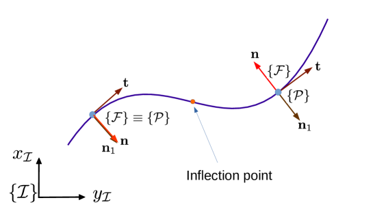
Figure 2.6: An illustration of Frenet-Serret $\{\mathcal{F}\}$ and Parallel Transport $\{\mathcal{P}\}$ frames in 2D. Notice how at the inflection point the normal vector $\bf n$ of the Frenet-Serret frame inverts its direction.

Remark 1.

Another way of propagating a P-T frame along the path is to use the algorithm proposed in [HM95]. While this algorithm is general and efficient for 3D, it is unnecessarily complicated for 2D curves.

2.3 Path following formulation

With the concepts and notation described above, the path following problem is stated next, see also Fig.2.3.
Path following problem in 2D: Given the 2-D spatial path $\mathcal{P}$ described by (5) and a vehicle with the kinematics model described by (2), derive a feedback control law for the vehicle’s inputs $(u,r)$ and possibly for $\dot{\gamma}$ or $\ddot{\gamma}$ so as to fulfill the following tasks:

1. Geometric task: steer the position error ${\bf e}\triangleq{\bf p}-{\bf p}_{\rm d}$ s.t.

   $$\lim_{t\to\infty}{\bf e}(t)={\bf 0},$$ (9)

   where ${\bf p}_{\rm d}$ is the inertial position of a “reference point” $P$ on the path, the temporal evolution of which can be chosen in a number of ways as discussed later.

2. Dynamic task: ensure that the vehicle’s forward speed tracks a positive desired speed profile $U_{\rm d}=U_{\rm d}(\gamma,t)$, i.e.

   $$\lim_{t\to\infty}u(t)-U_{\rm d}(t)=0.$$ (10)

In what follows, let $u_{\scriptscriptstyle{\mathcal{P}}}$ be the speed of the “reference point” $P$ with respect to the inertial frame, that is,

$$u_{\scriptscriptstyle{\mathcal{P}}}=\frac{\rm d{{\bf p}}_{\rm d}}{{\rm d}t}={\left\|{{\bf p}^{\prime}_{\rm d}(\gamma)}\right\|}\dot{\gamma}.$$ (11)

Should the vehicle achieve precise path following, both the vehicle and the point $P$ will move with the desired speed profile $U_{\rm d}$, i.e. $u=u_{\scriptscriptstyle{\mathcal{P}}}=U_{\rm d}$. In this case the dynamics task in (10) is equivalent to requiring

$$\lim_{t\to\infty}\dot{\gamma}(t)-v_{\rm d}(\gamma,t)=0,$$ (12)

where $v_{\rm d}$ is the desired speed profile for $\dot{\gamma}$, defined by

$$v_{\rm d}(\gamma,t)\triangleq\frac{1}{{\left\|{{\bf p}^{\prime}_{\rm d}(\gamma)}\right\|}}U_{\rm d}(\gamma,t).$$ (13)

In path following, the point $P$ on the path plays the role of a “reference point” for the vehicle to track. This point can be chosen as the nearest point to the vehicle [MS93], i.e. the orthogonal projection of the vehicle on the path (in case it is well defined), or can be initialized arbitrarily anywhere on the path with its evolution controlled through $\dot{\gamma}$ [LSP03, BF05] or $\ddot{\gamma}$ [AH07] to achieve the path following objectives. In the latter cases, $\dot{\gamma}$ or $\ddot{\gamma}$ are considered as the controlled input of the dynamics of the “reference point”, affording an extra freedom in the design of path following controllers.

2.4 Common principles of path following methods

Although there are a variety of path following methods described in the literature, most of them can be categorized as in Table 1. The first category includes the methods that aimed to stabilize the position error in a frame attached to a reference point point moving along the path (e.g. F-S or P-T frames), whereas the second category consists of the methods that aim to stabilize the position error in the vehicle’s body frame. The origin of the first method can be traced back to the work of [MS93] addressing the path following problem of unicycle-type and two-steering-wheels mobile robots. The core idea in this work was then adopted to develop more advanced path following algorithms in [LSP03, YLCA15, HRCP18]. Later, we shall see that Line-of-Sight (LOS), a well-known path following method and widely used in marine craft [FBS03] can be categorized in this group as well. The second approach was proposed by [AH07] and further developed in [AAJ13] to handle the vehicle’s input and state constraints.

Table 1: Principles of path following methods

	${\bf u}$	Principles
		Stabilizing ${\bf e}$ in path frames	Stabilizing ${\bf e}$ in the body frame
2D	$u,\psi$	[PAP91, FBS03, BF05, MAP09]
	$u,r$	[MS93, LSP03] [YLCA15, HRCP18]	[AH07][AAJ13]

3 Basic path following methods

In this section we study path following methods for vehicles whose motion is described by the kinematic model (2). In Section 4 we will extend the methods to the cases when the vehicle motion is subjected to external disturbances.

3.1 Methods based on stabilizing the path following error in the path frame

In this section we present a “unified formulation” that is simple but general enough to cover the path following methods in [MS93, LSP03, LSP06, BF05, FPG15, HRCP18]. The common principle behind these methods can be summarized in two steps:

• step 1: derive the dynamics of the path following error between the vehicle and the path in a path frame (e.g. F-S or P-T frame)

• step 2: drive these errors to zero using nonlinear control techniques to achieve path following, i.e. make the vehicle converge to and move along the path with a desired speed profile.

In order to have a unified formulation, instead of using the F-S frame as in [MS93, LSP03, LSP06] we use the P-T frame. The main advantage of the P-T frame in comparison with the F-S frame was discussed in Section 2.2, i.e. it avoids the singularity when the path has a vanishing second derivative, e.g. concave paths. Furthermore, the approach that we describe here is different from the one in [MS93, LSP03, LSP06] in that the formulation in this section applies to any path that is not necessarily parameterized by the arc-length.

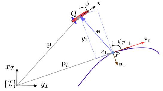
Figure 3.1: A geometric illustration of the methods in Section 3.1. $P$ is the “reference point” that the vehicle must track to achieve path following.

3.2 Derivation of the path following error

We now derive the dynamics of the path following errors (position and possibly orientation errors) between the vehicle and the path to be stabilized in order to achieve path following. The formulation is inspired by the work in [MS93, LSP03, BF05] and is presented next. Let $P$ be a point moving along the path that plays the role of a “reference point” for the vehicle to track so as to achieve path following. Let $\{\mathcal{P}\}$ be the P-T frame attached to this point defined by rotating the inertial frame by angle $\psi_{\scriptscriptstyle{\mathcal{P}}}$, where $\psi_{\scriptscriptstyle{\mathcal{P}}}$ is the angle that the tangent vector at $P$ makes with $x_{\mathcal{I}}$; see Fig. 3.1. Let ${\bf e}_{\scriptscriptstyle{\mathcal{P}}}\triangleq[s_{1},y_{1}]^{\top}\in\mathbb{R}^{2}$ be a vector defining the position error between the vehicle and the referene point $P$, where $s_{1}$ and $y_{1}$ are called along-track and cross-track errors, respectively. This vector can be viewed as the position vector of the vehicle expressed in $\{\mathcal{P}\}$. According to this definition, it is given by

$${\bf e}_{\scriptscriptstyle{\mathcal{P}}}=R^{\scriptscriptstyle{\mathcal{P}}}_{\scriptscriptstyle{\mathcal{I}}}(\psi_{\scriptscriptstyle{\mathcal{P}}})({\bf p}-{\bf p}_{\rm d}),$$ (14)

where ${\bf p}=[x,y]\in\mathbb{R}^{2}$ is the position of the vehicle, ${\bf p}_{\rm d}$ is given by (5) and $R^{\scriptscriptstyle{\mathcal{P}}}_{\scriptscriptstyle{\mathcal{I}}}\in SO(2)$ is the rotation matrix from $\left\{\mathcal{I}\right\}$ to $\{\mathcal{P}\}$, defined as

$$R^{\scriptscriptstyle{\mathcal{P}}}_{\scriptscriptstyle{\mathcal{I}}}(\psi_{\scriptscriptstyle{\mathcal{P}}})=\begin{bmatrix}\cos(\psi_{\scriptscriptstyle{\mathcal{P}}})&\sin(\psi_{\scriptscriptstyle{\mathcal{P}}})\\ -\sin(\psi_{\scriptscriptstyle{\mathcal{P}}})&\cos(\psi_{\scriptscriptstyle{\mathcal{P}}})\end{bmatrix}.$$ (15)

Note that $R^{\scriptscriptstyle{\mathcal{P}}}_{\scriptscriptstyle{\mathcal{I}}}(\psi_{\scriptscriptstyle{\mathcal{P}}})=[R^{\scriptscriptstyle{\mathcal{I}}}_{\scriptscriptstyle{\mathcal{P}}}(\psi_{\scriptscriptstyle{\mathcal{P}}})]^{\top}$. It is obvious that if ${\bf e}_{\scriptscriptstyle{\mathcal{P}}}\to\bf{0}$, then the geometrical task in the path following problem will be solved. Taking the time derivative of (14) yields

$$\dot{{\bf e}}_{\scriptscriptstyle{\mathcal{P}}}=[\dot{R}^{\scriptscriptstyle{\mathcal{I}}}_{\scriptscriptstyle{\mathcal{P}}}(\psi_{\scriptscriptstyle{\mathcal{P}}})]^{\top}({\bf p}-{\bf p}_{\rm d})+R^{\scriptscriptstyle{\mathcal{P}}}_{\scriptscriptstyle{\mathcal{I}}}(\psi_{\scriptscriptstyle{\mathcal{P}}})(\dot{{\bf p}}-\dot{{\bf p}}_{\rm d}).$$ (16)

Applying Lemma 5 (in the Appendix) for the first term of the previous equation we obtain

$$\dot{{\bf e}}_{\scriptscriptstyle{\mathcal{P}}}=-S(\boldsymbol{\omega}_{\scriptscriptstyle{\mathcal{P}}}){\bf e}_{\scriptscriptstyle{\mathcal{P}}}+R^{\scriptscriptstyle{\mathcal{P}}}_{\scriptscriptstyle{\mathcal{I}}}(\psi_{\scriptscriptstyle{\mathcal{P}}})\dot{{\bf p}}-R^{\scriptscriptstyle{\mathcal{P}}}_{\scriptscriptstyle{\mathcal{I}}}(\psi_{\scriptscriptstyle{\mathcal{P}}})\dot{{\bf p}}_{\rm d},$$ (17)

where $S(\boldsymbol{\omega}_{\scriptscriptstyle{\mathcal{P}}})\in\mathbb{R}^{2\times 2}$ is a skew symmetric matrix parameterized by $\boldsymbol{\omega}_{\scriptscriptstyle{\mathcal{P}}}=[r_{\scriptscriptstyle{\mathcal{P}}},0]^{\top}\in\mathbb{R}^{2}$ which is the angular velocity vector of $\{\mathcal{P}\}$ respect to $\left\{\mathcal{I}\right\}$, expressed in $\{\mathcal{P}\}$. Note that $r_{\scriptscriptstyle{\mathcal{P}}}$ satisfies the relation

$$r_{\scriptscriptstyle{\mathcal{P}}}=\kappa(\gamma)u_{\scriptscriptstyle{\mathcal{P}}},$$ (18)

where $u_{\scriptscriptstyle{\mathcal{P}}}$ is the total speed of $P$ given by (11) and $\kappa(\gamma)$ is the “signed” curvature of the path at $P$, given by

$$\kappa(\gamma)=\frac{x_{\rm d}^{\prime}(\gamma)y_{\rm d}^{\prime\prime}(\gamma)-x_{\rm d}^{\prime\prime}(\gamma)y_{\rm d}^{\prime}(\gamma)}{{\left\|{{\bf p}_{\rm d}^{\prime}(\gamma)}\right\|}^{3}}.$$ (19)

Note also that if $\gamma$ is the arc-length of the path then ${\left\|{{\bf p}^{\prime}_{\rm d}(\gamma)}\right\|}=1$. In this case, $u_{\scriptscriptstyle{\mathcal{P}}}=\dot{\gamma}$, i.e. the speed of the “reference point” equals the rate of change of the path length. Define

$$\psi_{\rm e}\triangleq\psi-\psi_{\scriptscriptstyle{\mathcal{P}}}$$ (20)

as the orientation error between the vehicle’s heading and the tangent to the path. Then,

$$R^{\scriptscriptstyle{\mathcal{P}}}_{\scriptscriptstyle{\mathcal{I}}}(\psi_{\scriptscriptstyle{\mathcal{P}}})\dot{{\bf p}}\stackrel{{\scriptstyle\eqref{eq: kinematics in 2D},\eqref{eq: RIP},\eqref{eq: psie}}}{{=}}\begin{bmatrix}u\cos(\psi_{\rm e})\\ u\sin(\psi_{\rm e})\end{bmatrix}.$$ (21)

Furthermore, letting ${\bf v}_{\scriptscriptstyle{\mathcal{P}}}\triangleq[u_{\scriptscriptstyle{\mathcal{P}}},0]^{\top}\in\mathbb{R}^{2}$ be the velocity of $P$ with respect to $\left\{\mathcal{I}\right\}$, expressed in $\{\mathcal{P}\}$, yields

$$R^{\scriptscriptstyle{\mathcal{P}}}_{\scriptscriptstyle{\mathcal{I}}}(\psi_{\scriptscriptstyle{\mathcal{P}}})\dot{{\bf p}}_{\rm d}={\bf v}_{\scriptscriptstyle{\mathcal{P}}}.$$ (22)

Substituting (21) and (22) in (17) we obtain the dynamics of the position error as

$$\dot{{\bf e}}_{\scriptscriptstyle{\mathcal{P}}}=-S(\boldsymbol{\omega}_{\scriptscriptstyle{\mathcal{P}}}){\bf e}_{\scriptscriptstyle{\mathcal{P}}}+\begin{bmatrix}u\cos(\psi_{\rm e})\\ u\sin(\psi_{\rm e})\end{bmatrix}-\begin{bmatrix}u_{\scriptscriptstyle{\mathcal{P}}}\\ 0\end{bmatrix}.$$ (23)

Furthermore, from (20) the dynamics of the orientation error are given by

$$\dot{\psi}_{\rm e}\stackrel{{\scriptstyle\eqref{eq: kinematics in 2D},\eqref{eq: angular velocity vector of P in I}}}{{=}}r-\kappa(\gamma)u_{\scriptscriptstyle{\mathcal{P}}}.$$ (24)

At this point, it should be clear that the geometric task in the path following problem, stated in Section 2.3, is equivalent to the problem of stabilizing the position error system (23), i.e. making ${\bf e}_{\scriptscriptstyle{\mathcal{P}}}(t)\to{\boldsymbol{0}}$ as $t\to\infty$. In what follows we will describe a number of path following methods available in the literature that solve this problem. These methods are categorized in Table 2. In Methods 1 and 3, the “reference point” is chosen as the orthogonal projection of the center of mass of the vehicle on the path, thus the along-track error $s_{1}(t)=0$ for all $t$. In this case, only the cross-track $y_{1}$ needs to be stabilized to fulfill the geometrical task. In contrast, in the other methods the “reference point” is initialized arbitrarily anywhere on the path and its evolution is controlled by assigning a proper law for $\dot{\gamma}$ so as to make the cross-track and along-track errors converge to zero. In all of the methods, in order to fulfill the dynamics task in the path following problem (see (10)), the linear speed of the vehicle is assigned with the desired speed profile, i.e. $u=U_{d}$.

Table 2: Methods proposed to stabilize ${\bf e}_{\scriptscriptstyle{\mathcal{P}}}$ to zero

PF Methods	Drive ${\bf e}_{\scriptscriptstyle{\mathcal{P}}}$ to zero by	References
Method 1	$u,r{\color[rgb]{1,1,1}\dot{\gamma},}$	[MS93]
Method 2	$u,r,\dot{\gamma}$	[LSP03]
Method 3	$u,\psi{\color[rgb]{1,1,1}\dot{\gamma},}$	[PAP91, FBS03, FPG15]
Method 4	$u,\psi,\dot{\gamma}$	[BF05]
Method 5	$u,r,\dot{\gamma}$	[YLCA15, HPJ20]

Remark 2.

In the formulation above, if $\gamma$ is the arc-length of the path, then in (19) ${\left\|{{\bf p}^{\prime}_{\rm d}(\gamma)}\right\|}=1$ and thus $u_{\scriptscriptstyle{\mathcal{P}}}=\dot{\gamma}$. In this case, the path following error system composed by (23) and (24) resembles the path following error system developed in [LSP03]; see equation (5) in [LSP03]. Notice that although parameterizing a path by its arc-length is convenient, this is not always possible; elliptical and sinusoidal curves are typical examples, [GAS06]. In the set-up above, the path parameter $\gamma$ is not necessarily the arc-length, thus making the formulation presented above applicable to any path.

Remark 3.

It is very important to note that in order to obtain $\dot{\psi}_{\rm e}$ in (24) ${\psi}_{\rm e}$ must be differentiable. This implies that $\psi$ and $\psi_{\scriptscriptstyle{\mathcal{P}}}$ must be differentiable as well. Although from a formulation standpoint there is no problem with this, in practice however, the heading sensors that measure $\psi$ normally return values in $[-\pi,\pi]$ or $[0,2\pi]$, thus the discontinuities happen when the angle changes between $-\pi$ and $\pi$ or between $0$ and $2\pi$. In this situation, to make $\psi$ and $\psi_{\scriptscriptstyle{\mathcal{P}}}$ continuous and differentiable we should open the domain of these angles to $\mathbb{R}$ before using them in path following algorithms involving in using $\psi_{\rm e}$. We suggest a simple algorithm to deal with this situation in the path following toolbox that shall be presented in Section 6.

3.2.1 Method 1 [MS93]: Achieve path following by controlling $(u,r)$

In this section we will describe the first method named as Method 1, proposed in [MS93], to solve the path following problem. The main objective is to derive a control strategy for $(u,r)$ to drive the position error in the systems (23) and (24) to zero. In this method, the “reference point” is chosen as the orthogonal projection of the real vehicle on the path, that is, the point on the path closest to the vehicle (if it is well-defined). With this strategy the along-track error is always zero, i.e. $s_{1}(t)=0$ for all $t$. Thus, we only need to stabilize the cross-track $y_{1}$ to zero to fulfill the geometry task. The dynamics of the cross-track error can be written explicitly from (23) as

$$\dot{y}_{1}=-r_{\scriptscriptstyle{\mathcal{P}}}s_{1}+u\sin(\psi_{\rm e})\stackrel{{\scriptstyle s_{1}=0}}{{=}}u\sin(\psi_{\rm e}).$$ (25)

Define

$$\tilde{\psi}=\psi_{\rm e}-\delta(y_{1},u),$$ (26)

where $\delta(y_{1},u)$ is a time differentiable design function that can be used to shape the manner in which the vehicle approaches the path. The design of $\delta(y_{1},u)$ must satisfy the following condition.

Condition 1 (for the design of $\delta(y_{1},u)$ [MS93, LSP03]).

1. $\delta(0,u)=0$ for all $u$.

2. $y_{1}u\sin(\delta(y_{1},u))\leq 0$ for all $y_{1},u$.

Taking the time derivative of (26) yields

$$\dot{\tilde{\psi}}\stackrel{{\scriptstyle\eqref{eq: dote_psi}}}{{=}}r-\kappa(\gamma)u_{\scriptscriptstyle{\mathcal{P}}}-\dot{\delta}.$$ (27)

Notice also that because ${s}_{1}(t)=0$ for all $t$, $u_{\scriptscriptstyle{\mathcal{P}}}$ in the above equation is obtained by solving the first equation in (23), yielding

$$u_{\scriptscriptstyle{\mathcal{P}}}=u\frac{\cos(\psi_{\rm e})}{1-\kappa(\gamma)y_{1}}.$$ (28)

We obtain the following theorem.

Theorem 3.1.

Consider a system composed by the dynamics of the cross-track error in (25) and the orientation error in (27). Let

$$u=U_{\rm d},$$ (29)

where $U_{\rm d}$ is the positive desired speed profile for the vehicle to track. Further let

$$r=\kappa(\gamma)u_{\scriptscriptstyle{\mathcal{P}}}+\dot{\delta}-k_{1}\tilde{\psi}-k_{2}y_{1}u\frac{\sin(\psi_{\rm e})-\sin(\delta)}{\tilde{\psi}},$$ (30)

where $k_{1},k_{2}>0$ are tuning parameters, $\kappa(\gamma)$ is defined in (19), $\psi_{\rm e}$ and $\tilde{\psi}$ are given by (20) and (26), respectively, $u_{\scriptscriptstyle{\mathcal{P}}}$ given by (28). Then, $y_{1}(t)$ and $\tilde{\psi}(t)$ converge to zero as $t\to\infty$.

Proof: See the Appendix - in Section 10.2.1.

Notice that because of Condition 1 once $y_{1},\tilde{\psi}\to 0$, then $\psi_{e}\to 0$ as well. This is true because we are assuming that the vehicle is under-actuated and has negligible lateral motion (that is, the total velocity vector is aligned with the body’s longitudinal axis). In this situation, the vehicle velocity’s vector will align itself with the tangent vector of the P-T frame. To satisfy Condition 1, $\delta(\cdot)$ can be chosen as

$$\delta(y_{1},u)=-\theta\tanh(k_{\delta}y_{1}u),$$ (31)

where $\theta\in(0,\pi/2)$ and $k_{\delta}>0$ [LSP06]. In summary, this path following method can be implemented with Algorithm 1.

Algorithm 1 PF algorithm using Method 1

1:For every time $t$ do:

2:procedure PF CONTROLLER

3:     Find $P$ - the point on the path closest to the vehicle

4:     Compute $y_{1}$ by (14), $\psi_{\rm e}$ by (20), and $\tilde{\psi}$ by (26)

5:     For inner-loop controllers (see Fig. 2.2):

6:       - Compute the desired vehicle’s forward speed by (29)

7:       - Compute the desired vehicle’s yaw rate given by (30)

8:end procedure

The implementation of line 3 in the algorithm is equivalent to solving an optimization problem to find $\gamma^{*}$, where

$$\gamma^{*}=~{}\underset{\gamma~{}\in~{}\Omega}{\operatorname{argmin}}{\left\|{{\bf p}-{\bf p}_{\rm d}(\gamma)}\right\|},$$ (32)

where ${\bf p}_{\rm d}(\gamma)$ is given by (5). Note also that the computation in Algorithm 1 associated with $\gamma$ uses $\gamma^{*}$, which is obtained by solving (32). In many cases, e.g. straight-line or circumference paths, $\gamma^{*}$ can be found analytically.

Remark 4.

Because the “reference point” on the path for the vehicle to track is chosen closest to the vehicle, there exists a singularity when $y_{1}=1/\kappa(\gamma)$ which stems from (28). This happens for example when the path is a circumference and the vehicle goes through the center of it.

3.2.2 Method 2 [LSP03]: Achieve path following by controlling $(u,r,\dot{\gamma})$

In this section we will describe the second method, named as Method 2, proposed by [LSP03] to solve the path following problem. The main objective is to derive a control law for $(u,r,\dot{\gamma})$ to drive the position and orientation errors in (23) and (24) to zero in order to achieve path following. In this method, instead of choosing the “reference point” on the path that is closest to the vehicle as in Method 1, this point can be initialized anywhere on the path, and its evolution is controlled by $\dot{\gamma}$ (to be defined later) in oder to eliminate the along-track error [LSP03]. In order to eliminate the cross-track and orientation errors, this method uses the same controller for $u,r$ as in Method 1. We now state the main result of this method, followed by a discussion on the intuition behind this result.

Theorem 3.2.

Consider the path following error system composed by (23) and (24). Let $u=U_{d}$ (as given by (29)), $r$ be given by (30), and

$$u_{\scriptscriptstyle{\mathcal{P}}}=u\cos(\psi_{\rm e})+k_{3}s_{1},$$ (33)

where $k_{3}>0$. Then, ${\bf e}_{\scriptscriptstyle{\mathcal{P}}}(t),\psi_{\rm e}(t)\to 0$ as $t\to\infty$.

Proof: See in Appendix - Section 10.2.2.

Recall that in (33) $s_{1}$ is the along-track error defined in (14). Because of the relation in (11), the control law for $\dot{\gamma}$ is given by

$$\dot{\gamma}=u_{\scriptscriptstyle{\mathcal{P}}}/{\left\|{{\bf p}^{\prime}_{\rm d}(\gamma)}\right\|},$$ (34)

where $u_{\scriptscriptstyle{\mathcal{P}}}$ is given by (33). In summary, the path following strategy of this method can be implemented as specified by Algorithm 2.

Algorithm 2 PF algorithm using Method 2

1:Initialize $\gamma(0)$

2:For every time $t$ do:

3:procedure PF CONTROLLER

4:     Compute the position and the orientation errors using (14) and (20).

5:     For inner-loop controllers (see Fig. 2.2):

6:       - Compute the desired vehicle’s forward speed using (29)

7:       - Compute the desired vehicle’s yaw rate given by (30)

8:     Compute $\dot{\gamma}$ in (34), then integrate it to update the value of $\gamma$

9:end procedure

The control law for $u_{\scriptscriptstyle{\mathcal{P}}}$ in (33) implies that if the vehicle is behind/ahead of the “reference point” $(s_{1}<0/s_{1}>0)$ then the “reference point” decreases/increases its speed. Intuitively, it aims to adjust the speed of the “reference point” to coordinate with the vehicle along the tangent axis of the P-T frame so as to reduce the along-track error to zero. Recall that in Method 1 proposed in [MS93] this error is always zero because the “reference point” is chosen as the point on the path that is closest to the vehicle. Compared with Method 1 this strategy has the following advantages: i) it doesn’t require an algorithm to find a point on the path that is closest to the vehicle and ii) it avoids the singularity that occurs in the method of [MS93] when $y_{1}=1/\kappa(\gamma)$.

3.2.3 Method 3 [FPG15]: Line-of-Sight path following

We now present the third method, named Method 3, to solve the path following problem. The main objective is to derive a control law for $(u,\psi)$ to drive the position error in the system (23) to zero in order to achieve path following. In the literature, this method is known as line-of-sight (LOS) method and was described in [FPG15]. Earlier work on LOS methods for straight-lines can be found in [PAP91, FBS03, AML13]. This method can be also found in [LWP16]. The LOS method is similar to Method 1 in the sense that the “reference point” is chosen as the orthogonal projection of the vehicle onto the path. Thus, the along track-error $s_{1}(t)=0$ for all $t$. However, it is different from Method 1 in that it derives a control law for the vehicle’s heading $\psi$ to achieve path following, instead of the heading rate $r$ as in Method 1. We recall from Method 1 that because $s_{1}(t)=0$ the dynamics of cross-track are given by (25). In the present method $\psi_{\rm e}$ is viewed as a “control input” whose control law must be chosen to stabilize the cross-track error to zero.

Theorem 3.3.

Consider the cross track error system described by (25). Let the vehicle’s forward speed $u$ be given by (29). Let the control law for $\psi_{e}$ is given by

$$\psi_{\rm e}=\arctan\left(-\frac{y_{1}}{\Delta_{\rm h}}\right),$$ (35)

where $\Delta_{\rm h}>0$ is a tuning parameter. Then, $y_{1}(t)\to 0$ as $t\to\infty$. Because of the relation in (20), the control law for the vehicle’s heading is given by

$$\psi=\underbrace{\psi_{\scriptscriptstyle{\mathcal{P}}}+\arctan\left(-\frac{y_{1}}{\Delta_{\rm h}}\right)}_{\psi_{\rm los}}.$$ (36)

Proof: See Section 10.2.3 of the Appendix.
 
In the literature, $\Delta_{\rm h}$ is often referred as the look-ahead distance [AML13, FPG15] and $\psi_{\rm los}$ is called the light-of-sight angle that the heading of the vehicle should reach to achieve path following. An illustration of the relation between these variables is shown in Fig. 3.2. Notice that $\Delta_{\rm h}$ can be time varying and used to shape the convergence behavior towards the tangent (longitudinal) axis of $\{\mathcal{P}\}$. The larger value of $\Delta_{\rm h}$, the slower will the convergence be, but this in turn will require less aggressive turning maneuvers in order for the vehicle to reach the path. In summary, the path following Method 3 can be implemented using Algorithm 3.

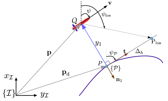
Figure 3.2: Geometric illustration of LOS method, where $y_{1}$ is the cross-tracking error.

Algorithm 3 PF algorithm using Method 3

1:For every time $t$ do:

2:procedure PF CONTROLLER

3:     Find $P$ - the point on the path closest to the vehicle

4:     For inner-loop controllers (see Fig. 2.2):

5:       - Compute the desired vehicle’s forward speed using (29)

6:       - Compute the desired vehicle’s heading angle using (36).

7:end procedure

Remark 5.

The control law for the steering angle of the vehicle in (36) can be rewritten in the Body frame as

$$\psi_{\mathcal{B}}=\psi_{e}+\arctan\left(-\frac{y_{1}}{\Delta_{\rm h}}\right),$$ (37)

where $\psi_{e}$ is given by (20).

It is interesting that this control law for the steering angle is equivalent to the one used in the autonomous car called Stanley who won the DARPA Grand Challenge - the competition for autonomous driving in unrehearsed off-road terrain in 2005 [TMD⁺07].

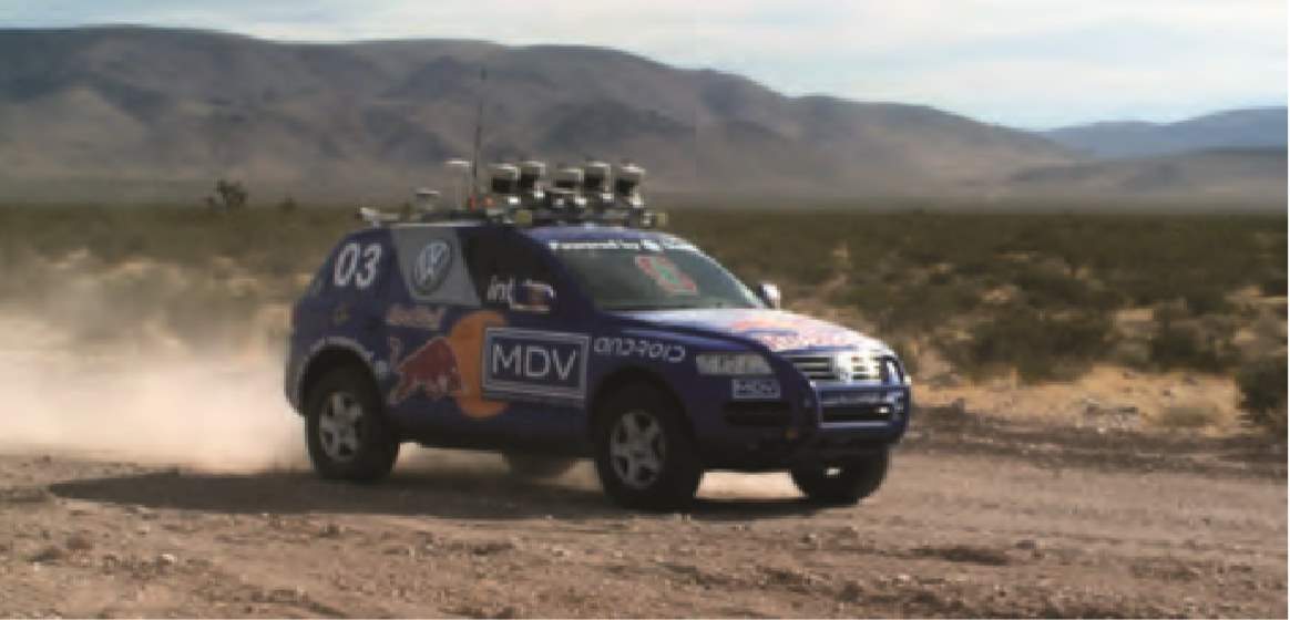
Figure 3.3: Stanley robotic car [TMD⁺07]

Remark 6.

The cross track error $y_{1}(t)$ in system (25) can also be driven to zero with the control law $\psi_{\rm e}$ given by

$$\psi_{\rm e}=\arcsin\left({\rm sat}\left(-\frac{1}{u}k_{1}y_{1}\right)\right)$$ (38)

with any $k_{1}>0$. In (38), $\rm sat(\cdot)$ is a saturation function that returns values in $[-1,1]$, thus guaranteeing that the $\arcsin$ function is well defined. With (38), the dynamics of the cross track error are given by

$$\dot{y}_{1}=-u~{}{\rm sat}\left(-\frac{1}{u}k_{1}y_{1}\right),$$

from which it is easy to see that $y_{1}(t)$ converges to zero as $t\to\infty$, [MAP09].

3.2.4 Method 4 [BF05]: Achieve path following by controlling $(u,\psi,\dot{\gamma})$

This path following method is described in [BF05] and has a similar principle with that in [LSP03, Rys03]. The idea behind this method is quite similar to that in Method 2; however, instead of achieving path following by controlling the heading rate $r$, the authors propose a control law for $\psi$.

Theorem 3.4.

Consider the position error system described by (23). Let the vehicle’s forward speed $u$ be given by (29), the speed of the “reference point” $P$ $u_{\scriptscriptstyle{\mathcal{P}}}$ be given by (33), and $\psi_{\rm e}$ given by (35). Then, ${\bf e}_{\scriptscriptstyle{\mathcal{P}}}={\bf 0}$ is UGAS.

Proof: See Section 10.2.4 in in the Appendix.
 
Because of relation (20) the control laws for the vehicle’s heading and $\dot{\gamma}$ are given by (36) and (34), respectively. The path following method can be implemented as specified in Algorithm 4. It can be seen from Algorithms 2 and 4 that the two are quite similar except that in the latter the vehicle is guided by controlling its heading, whereas in the former this is done by controlling its heading/yaw rate.

Algorithm 4 PF algorithm using Method 4

1:Initialize $\gamma(0)$

2:For every time $t$ do:

3:procedure PF CONTROLLER

4:     Compute the position errors $s_{1},y_{1}$ using (14)

5:     For inner-loop controllers (see Fig. 2.2):

6:       - Compute the desired vehicle’s forward speed using (29)

7:       - Compute the desired heading angle using (36).

8:     Compute $\dot{\gamma}$ using (34), then integrate it to update the value of $\gamma$

9:end procedure

Remark 7.

If the vehicle’s heading in Theorem 3.4 is replaced by (38), then the path following error ${\bf e}_{\scriptscriptstyle{\mathcal{P}}}$ converges to zero asymptotically as well. This idea was presented in [Rib13] and can be proved simply as in the proof of Theorem 3.4.

3.2.5 Method 5 [YLCA15, HPJ20]: NMPC-based path following

The path following methods we have studied so far are conceptually simple in terms of design and implementation; however, they do not take into account the vehicle’s physical constraints (e.g. maximum and minimum yaw rate). As a consequence, proper care must be taken to ensure that the resulting systems end up operating in a small region where the control law for the unconstrained system does not violate the constraints. In order to deal with the vehicle’s constraints explicitly, in this section we will present an optimization based control strategy called model predictive control to solve the path following problem [YLCA15, HRCP18, HPJ20].
First, define

$${\bf x}_{\scriptscriptstyle{\mathcal{P}}}\triangleq[{\bf e}_{\scriptscriptstyle{\mathcal{P}}}^{\top},\psi_{\rm e},\gamma]^{\top}\in\mathbb{R}^{4}$$

as the state of the complete path following system where the position error ${\bf e}_{\scriptscriptstyle{\mathcal{P}}}$ is defined by (14) and the orientation error is defined by (20). If we assign to the vehicle the desired speed profile, i.e. $u=U_{\rm d}$ then the dynamics of the complete path following system can be rewritten from (23) and (24) as

$$\begin{split}\dot{\bf x}_{\scriptscriptstyle{\mathcal{P}}}&={\bf f}({{\bf x}}_{\scriptscriptstyle{\mathcal{P}}},{\bf u}_{\scriptscriptstyle{\mathcal{P}}})\triangleq\left[\begin{matrix}-{\left\|{{\bf p}^{\prime}_{\rm d}(\gamma)}\right\|}v_{\gamma}\left(1-\kappa(\gamma)y_{1}\right)+U_{\rm d}\cos(\psi_{\rm e})\\ -\kappa(\gamma)s_{1}{\left\|{{\bf p}^{\prime}_{\rm d}(\gamma)}\right\|}v_{\gamma}+U_{\rm d}\sin(\psi_{\rm e})\\ r-\kappa(\gamma){\left\|{{\bf p}^{\prime}_{\rm d}(\gamma)}\right\|}v_{\gamma}\\ v_{\gamma}\end{matrix}\right],\\ \end{split}$$ (39)

where ${\bf u}_{\scriptscriptstyle{\mathcal{P}}}\triangleq[r,v_{\gamma}]^{\top}\in\mathbb{R}^{2}$ is the input of the system, which is constrained in the set $\mathbb{U}_{\scriptscriptstyle{\mathcal{P}}}$ given by

$$\mathbb{U}_{\scriptscriptstyle{\mathcal{P}}}\triangleq\{(r,v_{\gamma}):v_{\min}\leq v_{\gamma}\leq v_{\max},|r|\leq r_{\max}\}.$$ (40)

Here, $r_{\max}$ arises from the physical limitations of the vehicle while $v_{\min}$ and $v_{\max}$ are design parameters. In order for the path following problem to be solvable, the bounds on $v_{\gamma}$ can be chosen such that $v_{\min}\leq 0$ and

$$v_{\max}>v_{\rm d}^{*}\triangleq\max{(v_{\rm d})},$$ (41)

where $v_{\rm d}$ is given by (13). Intuitively, the conditions on the bounds of $v_{\gamma}$ ensure that the “reference point” on the path that the vehicle must track has enough speed to coordinate with the vehicle in order to achieve path following and also to track the desired speed profile $v_{\rm d}$. The main objective now is to find an MPC control law for ${\bf u}_{\scriptscriptstyle{\mathcal{P}}}$ to stabilize the position orientation errors in the system (39) to zero. To this end, we define a finite horizon open loop optimal control problem (FOCP) that the MPC solves at every sampling time as follows:

Definition 3.5.

FOCP-1:

$${\min_{\bar{\bf u}_{\scriptscriptstyle{\mathcal{P}}}{}(\cdot)}}~{}J_{\scriptscriptstyle{\mathcal{P}}}\left({{\bf x}}_{\scriptscriptstyle{\mathcal{P}}}(t),\bar{\bf u}_{\scriptscriptstyle{\mathcal{P}}}{}(\cdot)\right)$$ (42)

subject to

$${\dot{{\bar{\bf x}}}}_{\scriptscriptstyle{\mathcal{P}}}(\tau)={\bf f}_{\scriptscriptstyle{\mathcal{P}}}({\bar{\bf x}}_{\scriptscriptstyle{\mathcal{P}}}{(\tau)},\bar{\bf u}_{\scriptscriptstyle{\mathcal{P}}}{(\tau)}),\tau\in\left[t,t+T_{\rm p}\right],\quad{\bar{\bf x}}_{\scriptscriptstyle{\mathcal{P}}}{(t)}={\bf x}_{\scriptscriptstyle{\mathcal{P}}}(t),$$ (43a)

$$\bar{\bf u}_{\scriptscriptstyle{\mathcal{P}}}{(\tau)}\in\mathbb{U}_{\scriptscriptstyle{\mathcal{P}}},\qquad\qquad\tau\in\left[t,t+T_{\rm p}\right],$$ (43b)

$$\left(\bar{{\bf e}}_{\scriptscriptstyle{\mathcal{P}}}(\tau),\bar{\psi}_{\rm e}(\tau)\right)\in\mathbb{E}_{\scriptscriptstyle{\mathcal{P}}},\quad\tau\in\left[t,t+T_{\rm p}\right]$$ (43c)

with

$$J_{\scriptscriptstyle{\mathcal{P}}}\left({\bf x}_{\scriptscriptstyle{\mathcal{P}}}(t),\bar{\bf u}_{\scriptscriptstyle{\mathcal{P}}}{}(\cdot)\right)\triangleq\int_{t}^{t+T_{\rm p}}{\left\|{\begin{bmatrix}\bar{{\bf e}}_{\scriptscriptstyle{\mathcal{P}}}(\tau)\\ \bar{\psi}_{\rm e}(\tau)\end{bmatrix}}\right\|}_{Q}+{\left\|{\bar{{\bf u}}_{\rm a}(\tau)}\right\|}_{R}~{}{\rm d}\tau+F_{\scriptscriptstyle{\mathcal{P}}}\left(\bar{{\bf e}}_{\scriptscriptstyle{\mathcal{P}}}(t+T_{\rm p}),\bar{\psi}_{\rm e}(t+T_{\rm p})\right),$$

where $Q\in\mathbb{R}^{3\times 3},R\in\mathbb{R}^{2\times 2}$ are positive definite matrices, and the notation $||{\bf x}||_{Q}={\bf x}^{\rm T}Q{\bf x}$ for any ${\bf x}\in R^{n}$ and $Q\in\mathbb{R}^{n\times n}$. The cost associated with the input is defined by

$${\bf u}_{\rm a}=\begin{bmatrix}U_{\rm d}\cos(\psi_{\rm e})-{\left\|{{\bf p}^{\prime}_{\rm d}(\gamma)}\right\|}v_{\gamma}\\ r-\kappa(\gamma){\left\|{{\bf p}^{\prime}_{\rm d}(\gamma)}\right\|}v_{\gamma}\end{bmatrix}.$$ (44)

In the FOCP-1, we use the bar notation to denote the predicted variables and to differentiate them from the actual variables which do not have a bar. Specifically, ${\bar{\bf x}}_{\scriptscriptstyle{\mathcal{P}}}(\tau)$ is the predicted trajectory of the state ${\bf x}_{\scriptscriptstyle{\mathcal{P}}}$, computed using the dynamic model (39) and the initial condition at the time $t$, driven by the input $\bar{\bf u}_{\scriptscriptstyle{\mathcal{P}}}{(\tau)}~{}\text{with}~{}\tau\in[t,t+T_{\rm p}]$ over the prediction horizon $[t,t+T_{\rm p}]$. The first cost of $J_{\scriptscriptstyle{\mathcal{P}}}(\cdot)$ is associated with the geometrical task, whereas the choice of ${\bf u}_{\rm a}$ in the argument of the cost function to be minimized is motivated by the fact that once ${\bf e}_{\scriptscriptstyle{\mathcal{P}}}$ and $\psi_{\rm e}$ $\to{0}$, ${\bf u}_{\rm a}\to\boldsymbol{0}$ as well. $\mathbb{E}_{\scriptscriptstyle{\mathcal{P}}}$ and $F_{\scriptscriptstyle{\mathcal{P}}}$ represent the terminal constraints (the terminal set and the terminal cost, respectively), that should be designed appropriately to guarantee “recursive feasibility” and “stability” of the MPC scheme [YLCA15].
In the MPC scheme, the FOCP-1 is repeatedly solved at every discrete sampling instant $t_{i}=iT_{\rm s}$, $i\in\mathbb{N}_{+}$, where $T_{\rm s}$ is a sampling interval. Let $\bar{\bf u}_{\scriptscriptstyle{\mathcal{P}}}{}^{*}(\tau),\tau\in[t,t+T_{\rm p}],$ be the optimal solution of the FOCP-1. Then, the MPC control law ${\bf u}_{\scriptscriptstyle{\mathcal{P}}}(\cdot)$ is defined by

$${\bf u}_{\scriptscriptstyle{\mathcal{P}}}(t)=\bar{\bf u}_{\scriptscriptstyle{\mathcal{P}}}^{*}{(t)},~{}t\in[t_{i},t_{i}+T_{\rm s}].$$ (45)

In summary, the MPC strategy for the path following problem can be implemented in Algorithm 5.

Algorithm 5 PF algorithm using Method 5

1:Initialize $\gamma(0)$

2:For every time $t$ do:

3:procedure PF CONTROLLER

4:     Compute the path following errors $s_{1},y_{1},\psi_{\rm e}$ using (14) and (20)

5:     Solve the FOCP-1 and apply the MPC control law (45) to obtain optimal $r,v_{\gamma}$

6:     For inner-loop controllers (see Fig. 2.2):

7:       - Compute the desired vehicle’s forward speed using (29)

8:       - The optimal $r$ is used as the desired vehicle’s heading rate

9:     Iterate $\gamma$ with the optimal input $v_{\gamma}$ to update $\gamma$

10:end procedure

Another way of ensuring stability for the path following error system (39) without using the terminal constraints is to impose a “contractive constraint” in the FOCP-1, see [HPJ20]. The “contractive constraint” in the reference is designed based on the knowledge of an existing global nonlinear stablizing controller for the path following error system, and is advantageous over the NMPC scheme in [YLCA15] in the sense that the origin of path following error is globally asymtotical stable. However, locally, with the NMPC scheme in [YLCA15], the path following error might converge to zero faster.

Remark 8.

While using the terminal constraints in [YLCA15] and the contractive constraint in [HPJ20] are appealing from a theoretical standpoint, for the simplicity in design and implementation in practice they are normally excluded from the finite optimal control problem. In this situation, it is well-known that the convergence of the path following error is guaranteed if the prediction horizon $T_{\rm p}$ is chosen sufficiently large [JH05, MRRS00]. However, it requires effort in tuning the prediction horizon to achieve stability.

Remark 9.

Nowadays there are a variety of tools that can support solving the nonlinear optimization problem like FOCP-1. Typical tools that are widely used in MPC’s work include Casadi [AGH⁺19], which was used in the work of [HPJ20] and in the simulation toolbox of the present paper, ACADO [HFD11], which was used in the work of [BZAF19], or MATLAB optimization toolbox (fmincon function).

3.3 Methods based on stabilizing the path following error in the body frame

3.3.1 Method 6 [AH07]: Achieve path following by controlling $(u,r,\ddot{\gamma})$

We now describe the second approach to the path following problem. It is different from the methods proposed in Section 3.1 in that the position error between the vehicle and the path is formulated in the vehicle’s body frame $\{\mathcal{B}\}$, instead of a path frame, [AH07, Van07]. A geometric illustration of this path following method is shown in Fig 3.4.

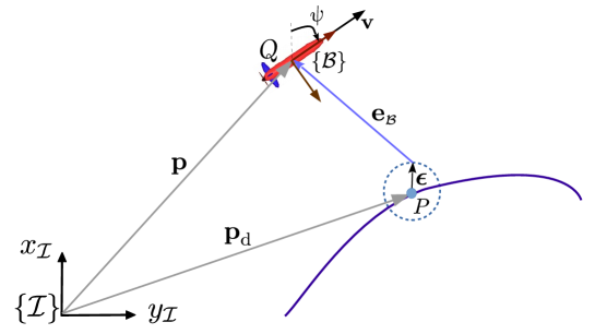
Figure 3.4: Geometric illustration of path following Method 6 [AH07]

First let $P$, whose coordinate is specified by ${\bf p}_{\rm d}(\gamma)$, be the “reference point” on the path that the vehicle should track to achieve path following. Define

$$\begin{split}{\bf e}_{\scriptscriptstyle{\mathcal{B}}}=R^{\scriptscriptstyle{\mathcal{B}}}_{\scriptscriptstyle{\mathcal{I}}}(\psi)({\bf p}-{\bf p}_{\rm d})-{\boldsymbol{\epsilon}}\end{split}$$ (46)

as the position error between the vehicle and the path resolved in the vehicle’s body frame $\left\{\mathcal{B}\right\}$, where ${\boldsymbol{\epsilon}}$ is an arbitrarily small non-zero constant vector and

$$R^{\scriptscriptstyle{\mathcal{B}}}_{\scriptscriptstyle{\mathcal{I}}}(\psi)=\begin{bmatrix}\cos(\psi)&\sin(\psi)\\ -\sin(\psi)&\cos(\psi)\\ \end{bmatrix}$$ (47)

is the rotation matrix from the inertial frame $\left\{\mathcal{I}\right\}$ to the body frame $\left\{\mathcal{B}\right\}$. The reason for introducing ${\boldsymbol{\epsilon}}$ will become clear later. By definition, if ${\bf e}_{\scriptscriptstyle{\mathcal{B}}}$ can be driven to zero then the vehicle will converge to the ball centered at the point $P$ with radius ${\left\|{\boldsymbol{\epsilon}}\right\|}$, which implies that the vehicle will converge to a neighborhood of the path that can be made arbitrarily small by choosing the size of $\boldsymbol{\epsilon}$. Taking the time derivative of (46) and using (2) and the fact that $R^{\scriptscriptstyle{\mathcal{I}}}_{\scriptscriptstyle{\mathcal{B}}}(\psi)=[R^{\scriptscriptstyle{\mathcal{B}}}_{\scriptscriptstyle{\mathcal{I}}}(\psi)]^{\top}$ yields

$$\dot{{\bf e}}_{\scriptscriptstyle{\mathcal{B}}}=[\dot{R}^{\scriptscriptstyle{\mathcal{I}}}_{\scriptscriptstyle{\mathcal{B}}}(\psi)]^{\top}({\bf p}-{\bf p}_{\rm d})+R^{\scriptscriptstyle{\mathcal{B}}}_{\scriptscriptstyle{\mathcal{I}}}(\psi)(\dot{{\bf p}}-\dot{{\bf p}}_{\rm d})$$

Using Lemma 5 in the Appendix for the first term, and expanding the previous equation we obtain

$$\begin{split}\dot{{\bf e}}_{\scriptscriptstyle{\mathcal{B}}}&=−S(\boldsymbol{\omega}){{\bf e}}_{\scriptscriptstyle{\mathcal{B}}}−S({\boldsymbol{\omega}}){\boldsymbol{\epsilon}}+{\bf v}−R^{\scriptscriptstyle{\mathcal{B}}}_{\scriptscriptstyle{\mathcal{I}}}(\psi){\bf p}^{\prime}_{\rm d}(\gamma)\dot{\gamma}\\ &=−S(\boldsymbol{\omega}){{\bf e}}_{\scriptscriptstyle{\mathcal{B}}}+\Delta{\bf u}−R^{\scriptscriptstyle{\mathcal{B}}}_{\scriptscriptstyle{\mathcal{I}}}(\psi){\bf p}^{\prime}_{\rm d}(\gamma)\dot{\gamma},\end{split}$$ (48)

where ${\boldsymbol{\omega}}=[r,0]^{\top}\in\mathbb{R}^{2}$ is the angular velocity vector of $\left\{\mathcal{B}\right\}$ respect to $\left\{\mathcal{I}\right\}$, expressed in $\left\{\mathcal{B}\right\}$, ${\bf u}=[u,r]$ and ${\Delta}=\begin{bmatrix}1&\epsilon_{2}\\ 0&\text{-}\epsilon_{1}\end{bmatrix}$. To address the dynamic task stated in (12), define

$$e_{\gamma}=\dot{\gamma}-v_{\rm d}$$ (49)

as the tracking error for the speed of the path parameter. By definition, if $e_{\gamma}$ can be driven to zero then the dynamics task is fulfilled. The dynamics of this error is given by

$$\dot{e}_{\gamma}=\ddot{\gamma}-\dot{v}_{\rm d}.$$ (50)

Let ${\bf x}=[{\bf e}^{\top}_{\scriptscriptstyle{\mathcal{B}}},e_{\gamma}]^{{\rm T}}\in\mathbb{R}^{3}$ be the complete path following error vector. From (48) and (50), the dynamics of the path following error vector can be expressed as

$$\dot{\bf x}=\left[\begin{matrix}−S(\boldsymbol{\omega}){{\bf e}}_{\scriptscriptstyle{\mathcal{B}}}+\Delta{\bf u}−R^{\scriptscriptstyle{\mathcal{B}}}_{\scriptscriptstyle{\mathcal{I}}}(\psi){\bf p}^{\prime}_{\rm d}(\gamma)\dot{\gamma}\\ \ddot{\gamma}-\dot{v}_{\rm d}\end{matrix}\right].$$ (51)

Theorem 3.6.

Consider the path following error system described by (51). Then, the control law for ${\bf u}$ and $\ddot{\gamma}$ given by

$${\bf u} =\bar{\Delta}\left(R^{\scriptscriptstyle{\mathcal{B}}}_{\scriptscriptstyle{\mathcal{I}}}(\psi){\bf p}^{\prime}_{\rm d}(\gamma)v_{\rm d}-K_{\rm p}{{\bf e}}_{\scriptscriptstyle{\mathcal{B}}}\right)$$ (52a)

$$\ddot{\gamma} =-k_{\gamma}e_{\gamma}+{\bf e}^{\top}_{\scriptscriptstyle{\mathcal{B}}}R^{\scriptscriptstyle{\mathcal{B}}}_{\scriptscriptstyle{\mathcal{I}}}({\psi}){\bf p}^{\prime}_{\rm d}(\gamma)+\dot{v}_{\rm d},$$ (52b)

render the origin of ${\bf x}$ GES, where $\bar{\Delta}=\Delta^{\top}(\Delta\Delta^{\top})^{-1}$, $K_{\rm p}$ is a positive definite matrix with appropriate dimension, and $k_{\gamma}>0$.

In summary, this path following method can be implemented as described in Algorithm 6.

Algorithm 6 PF Algorithm using Method 6

1:Initialize $\gamma(0)$ and $\dot{\gamma}(0)$

2:For every sampling interval, repeat the following procedure:

3:procedure PF CONTROLLER

4:     Compute the position error ${\bf e}_{\scriptscriptstyle{\mathcal{B}}}$ using (46) and the tracking error $e_{\gamma}$ using (49).

5:     For inner-loop controllers (see Fig. 2.2):

6:       - Compute the desired vehicle’s forward speed and yaw-rate using (52a)

7:     Compute $\ddot{\gamma}$ using (52b), then integrate it to update the value of $\gamma$

8:end procedure

Proof: See Section 10.2.5 in the Appendix.

Remark 10.

In (52) we can control the evolution of the “reference point” by assigning $\dot{\gamma}=v_{\rm d}$, instead of using the control law for $\ddot{\gamma}$, as in (52b). It can be easily shown that the origin of the path following error system is still GES as well. However, making $\dot{\gamma}=v_{\rm d}$ implies that the “reference point” moves without taking into consideration the state of the vehicle. In other words, in this case the vehicle tracks a pure trajectory and this might demand more aggressive manoeuvres.

Remark 11.

It is worth noticing that this method is not only applicable to the kinematic model (2) but also to the dynamics model of quad-rotor drone. For further details we refer the reader to the work presented in [Jac21].

3.3.2 Method 7 [AAJ13]: NMPC-based path following

In this section, we will describe the path following NMPC scheme in [AAJ13]. This scheme borrows from the formulation in Section 3.3.1. Using this formalism, path following is achieved by deriving an NMPC control law for $(u,r,\dot{\gamma})$ to i) drive the position error ${\bf e}_{\scriptscriptstyle{\mathcal{B}}}$ whose dynamics described by (48) to zero and also to ii) ensure that $\dot{\gamma}$ converges to $v_{\rm d}$ to fulfill the dynamics task in (12). For this purpose, define

$${\bf x}_{\scriptscriptstyle{\mathcal{B}}}\triangleq[{\bf e}^{\top}_{\scriptscriptstyle{\mathcal{B}}},\psi,\gamma]^{\top}\in\mathbb{R}^{4},\quad{\bf u}_{\scriptscriptstyle{\mathcal{B}}}\triangleq[u,r,v_{\gamma}]^{\top}\in\mathbb{R}^{3}$$ (53)

as the state and input of the complete path following system, respectively. Note that similar to the NMPC scheme in Method 5 we let $v_{\gamma}=\dot{\gamma}$ for convenience of presentation. Note also that in the present NMPC scheme, the vehicle’s speed is naturally optimized through the NMPC scheme, whereas with the NMPC scheme in Method 5, it is assigned directly by the desired speed profile $U_{\rm d}$. Because the vehicle’s speed is constrained due to the vehicle’s physical limitations, we define a constraint set for ${\bf u}_{\scriptscriptstyle{\mathcal{B}}}$ in (53) as

$$\mathbb{U}_{\scriptscriptstyle{\mathcal{B}}}\triangleq\mathbb{U}_{\scriptscriptstyle{\mathcal{P}}}\times\{u:u_{\min}\leq u\leq u_{\max}\},$$ (54)

where $\mathbb{U}_{\scriptscriptstyle{\mathcal{P}}}$ given by (40) and the bounds on the vehicle’s speed vary according to the physical constraints of the vehicle. The dynamics of the complete path following state can be rewritten from (2) and (48) as

$$\dot{{\bf x}}_{\scriptscriptstyle{\mathcal{B}}}={{\bf f}}_{\scriptscriptstyle{\mathcal{B}}}({\bf x}_{\scriptscriptstyle{\mathcal{B}}},{\bf u}_{\scriptscriptstyle{\mathcal{B}}})\begin{bmatrix}−S(\boldsymbol{\omega}){{\bf e}}_{\scriptscriptstyle{\mathcal{B}}}+\Delta{\bf u}−R^{\scriptscriptstyle{\mathcal{B}}}_{\scriptscriptstyle{\mathcal{I}}}(\psi){\bf p}^{\prime}_{\rm d}(\gamma)v_{\gamma}\\ r\\ v_{\gamma}\end{bmatrix},$$ (55)

The objective of the NMPC scheme is to find an optimal control strategy for ${\bf u}_{\scriptscriptstyle{\mathcal{B}}}$ to drive the position error ${\bf e}_{\scriptscriptstyle{\mathcal{B}}}$ and the speed tracking error $(v_{\gamma}-v_{\rm d})$ to zero. To this end, we now define a FOCP that the NMPC solves at every sampling time as follows:

Definition 3.7.

FOCP-2:

$${\min_{\bar{\bf u}_{\scriptscriptstyle{\mathcal{B}}}{}(\cdot)}}~{}J_{\scriptscriptstyle{\mathcal{B}}}\left({{\bf x}}_{\scriptscriptstyle{\mathcal{B}}}(t),\bar{\bf u}_{\scriptscriptstyle{\mathcal{B}}}{}(\cdot)\right)$$ (56)

subject to

$${\dot{\bar{{\bf x}}}_{\scriptscriptstyle{\mathcal{B}}}}(\tau)={\bf f}_{\scriptscriptstyle{\mathcal{B}}}(\bar{{\bf x}}_{\scriptscriptstyle{\mathcal{B}}}{(\tau)},\bar{\bf u}_{\scriptscriptstyle{\mathcal{B}}}{(\tau)}),\tau\in\left[t,t+T_{\rm p}\right],\quad{\bar{{\bf x}}}_{\scriptscriptstyle{\mathcal{B}}}{(t)}={{\bf x}}_{\scriptscriptstyle{\mathcal{B}}}(t),$$ (57a)

$$\bar{\bf u}_{\scriptscriptstyle{\mathcal{B}}}{(\tau)}\in\mathbb{U}_{\scriptscriptstyle{\mathcal{B}}},\quad\tau\in\left[t,t+T_{\rm p}\right],$$ (57b)

$$\bar{{\bf e}}_{\scriptscriptstyle{\mathcal{B}}}(\tau)\in\mathbb{E}_{\scriptscriptstyle{\mathcal{B}}},\quad\tau\in\left[t,t+T_{\rm p}\right].$$ (57c)

with

$$J_{\scriptscriptstyle{\mathcal{B}}}\left({\bf x}_{\scriptscriptstyle{\mathcal{B}}}(t),\bar{\bf u}_{\scriptscriptstyle{\mathcal{B}}}{}(\cdot)\right)\triangleq\int_{t}^{t+T_{\rm p}}{\left\|{\bar{{\bf e}}_{\scriptscriptstyle{\mathcal{B}}}(\tau)}\right\|}_{Q}+{\left\|{{\bf u}_{\rm b}(\tau)}\right\|}_{R}+{\left\|{v_{\gamma}(\tau)-v_{\rm d}(\tau)}\right\|}_{O}~{}{\rm d}\tau+F_{\scriptscriptstyle{\mathcal{B}}}(\bar{{\bf e}}_{\scriptscriptstyle{\mathcal{B}}}(t+T_{\rm p}))$$

where $Q,R,O\succ 0$ and

$${\bf u}_{\rm b}=\Delta{\bf u}−R^{\scriptscriptstyle{\mathcal{B}}}_{\scriptscriptstyle{\mathcal{I}}}(\psi){\bf p}^{\prime}_{\rm d}(\gamma)v_{\gamma}.$$ (58)

In the FOCP, we use the bar notation to denote the predicted variables, to differentiate them from the actual variables which do not have a bar. Specifically, ${\bar{\bf x}}_{\scriptscriptstyle{\mathcal{B}}}(\tau)$ is the predicted trajectory of ${\bf x}_{\scriptscriptstyle{\mathcal{B}}}$, using the dynamic model (55) and their perspective initial condition at time $t$, driven by the input $\bar{\bf u}_{\scriptscriptstyle{\mathcal{B}}}{(\tau)}~{}\text{with}~{}\tau\in[t,t+T_{\rm p}]$ over the prediction horizon $T_{\rm p}$. $\mathbb{E}_{\scriptscriptstyle{\mathcal{B}}}$ and $F_{\scriptscriptstyle{\mathcal{B}}}$ are called terminal set and terminal cost, respectively, to be designed appropriately to guarantee “recursive feasibility” and “stability” of the NMPC scheme [AAJ13]. The choice of ${\bf u}_{\rm b}$ in the cost function to be minimized is motivated by the fact that once ${\bf e}_{\scriptscriptstyle{\mathcal{B}}}\to\boldsymbol{0}$, ${\bf u}_{\rm b}\to\boldsymbol{0}$ as well.
In the NMPC scheme, the FOCP-2 is repeatedly solved at every discrete sampling instant $t_{i}=iT_{\rm s}$, $i\in\mathbb{N}_{+}$, where we recall that $T_{\rm s}$ is a sampling interval. Let $\bar{\bf u}_{\scriptscriptstyle{\mathcal{B}}}{}^{*}(\tau),\tau\in[t,t+T_{\rm p}],$ be the optimal solution of the FOCP-2. Then, the NMPC control law ${\bf u}_{\scriptscriptstyle{\mathcal{B}}}(\cdot)$ is defined as

$${\bf u}_{\scriptscriptstyle{\mathcal{B}}}(t)=\bar{\bf u}_{\scriptscriptstyle{\mathcal{B}}}^{*}{(t)},~{}t\in[t_{i},t_{i}+T_{\rm s}].$$ (59)

In summary the NMPC scheme can be implemented as in Algorithm 7.

Algorithm 7 PF algorithm using Method 7

1:Initialize $\gamma(0)$

2:For every time $t$ do:

3:procedure PF CONTROLLER

4:     Compute the path following errors $s_{1},y_{1},\psi_{\rm e}$ using (14) and (20)

5:     Solve the FOCP-2 and apply the NMPC control law (45) to obtain optimal values of $u,r,v_{\gamma}$

6:     For inner-loop controllers (see Fig. 2.2):

7:       - the optimal $u$ is used as the desired vehicle’s forward speed.

8:       - the optimal $r$ is used as the desired vehicle’s heading rate.

9:     Iterate $\gamma$ with the optimal input $v_{\gamma}$ to update the value of $\gamma$

10:end procedure

Note that for simplicity of design and implementation we can exclude the terminal constraints above from the finite optimal control problem. In this situation, we recall that the convergence of the path following error is guaranteed if the prediction horizon $T_{\rm p}$ is chosen sufficiently large [JH05, MRRS00].

4 Path following methods in the presence of external disturbances

In the previous section, we described a number of path following methods for the nominal kinematic model (2). We now discuss how these methods can be extended to the cases when the vehicle maneuvers in an environment where unknown constant external disturbances e.g. wind in the case of UAVs or ocean currents in the case of AMVs are present. In this situation, the vehicle kinematic model in (2) can be extended as

$$\begin{split}\dot{x}&=u\cos(\psi)+v_{\rm cx}\\ \dot{y}&=u\sin(\psi)+v_{\rm cy}\\ \dot{\psi}&=r\\ \dot{v}_{\rm cx}&=0,\quad\dot{v}_{\rm cy}=0,\end{split}$$ (60)

where $v_{\rm cx},v_{\rm cy}$ are two components of ${\bf v}_{\rm c}$, i.e. ${\bf v}_{\rm c}=[v_{\rm cx},v_{\rm cy}]^{\top}\in\mathbb{R}^{2}$ - the vector that describes the influence of the external unknown disturbance in the inertial frame. It is important to note that in (2) $u$ is the longitudinal/surge speed measured with respect to the fluid. In the literature, the effect of a constant disturbance can be eliminated using two approaches. The first is to add an integral term in the path following control laws. This is simple but only applicable for straight-line paths. The second uses estimates of the disturbances and is applicable to every path. These approaches are presented next.

Remark 12.

Note that in the present paper we only address the cases where the external disturbance is a constant. For more general cases where the disturbance is an unknown sinusoidal signal the reader is referred to the work in [Gho17] and [Gho21]. The idea behind this work is to use an adaptive internal model to estimate the disturbance and then use it in a combination with the path following Method 6 to cancel out the disturbance effect.

4.1 Path following with integral terms

The LOS type path following methods presented in Section 3.2.3 can be extended in a simple manner to handle constant external disturbances. For this purpose, we first re-derive the dynamics of the path following error in the presence of an external disturbance. Given the kinematic model in (60) and following the procedure described in Section 3.2, it can be shown that the dynamics of the position error ${\bf e}_{\scriptscriptstyle{\mathcal{P}}}$ (expressed in the P-T frame) are given by

$$\dot{{\bf e}}_{\scriptscriptstyle{\mathcal{P}}}=-S(\boldsymbol{\omega}_{\scriptscriptstyle{\mathcal{P}}}){\bf e}_{\scriptscriptstyle{\mathcal{P}}}+\begin{bmatrix}u\cos(\psi_{\rm e})\\ u\sin(\psi_{\rm e})\end{bmatrix}-\begin{bmatrix}u_{\scriptscriptstyle{\mathcal{P}}}\\ 0\end{bmatrix}+R^{\scriptscriptstyle{\mathcal{P}}}_{\scriptscriptstyle{\mathcal{I}}}(\psi_{\scriptscriptstyle{\mathcal{P}}}){\bf v}_{\rm c}.$$ (61)

Recall that ${\bf e}_{\scriptscriptstyle{\mathcal{P}}}=[s_{1},y_{1}]^{\top}$ is defined by (14) while the orientation error $\psi_{\rm e}$ is defined by (20). Note that in the above equation, the last term represents the influence of the external disturbance ${\bf v}_{\rm c}$. We will show that this disturbance can be eliminated by adding an integral term in the LOS methods provided that the following assumptions are satisfied

Assumption 4.1.

The “reference point” on the path for the vehicle to track is chosen as the closet point to the vehicle, i.e. the along-track error $s_{1}(t)=0$ for all $t$.

With the above assumption the dynamics of the cross track can be rewritten from (61) as

$$\dot{y}_{1}=u\sin(\psi_{\rm e})+v_{\rm cy}^{\scriptscriptstyle{\mathcal{P}}},$$ (62)

where

$$v_{\rm cy}^{\scriptscriptstyle{\mathcal{P}}}\triangleq-\sin(\psi_{\scriptscriptstyle{\mathcal{P}}})v_{\rm cx}+\cos(\psi_{\scriptscriptstyle{\mathcal{P}}})v_{\rm cy}.$$ (63)

is the external disturbance acting along the coordinate $x_{\scriptscriptstyle{\mathcal{P}}}$ of the P-T frame. If ${\bf v}_{\rm c}$ and $\psi_{\scriptscriptstyle{\mathcal{P}}}$ are constant, then the unknown disturbance $v_{\rm cy}^{\scriptscriptstyle{\mathcal{P}}}$ is constant as well. Thus, by adding an integral terms in the LOS methods presented in Section 3.2.3, the effect of $v_{\rm cy}^{\scriptscriptstyle{\mathcal{P}}}$ on the cross-track error can be eliminated.

Theorem 4.2.

Consider the dynamics of the cross-track error given by (62) where $v_{\rm cy}^{\scriptscriptstyle{\mathcal{P}}}$ is assumed to constant (i.e. the path is a straight-line). The control law for $\psi_{\rm e}$ given by

$$\begin{split}\psi_{\rm e}&=\arctan\left(-\frac{y_{1}+\sigma y_{\rm int}}{\Delta_{\rm h}}\right)\quad\text{and}\\ \dot{y}_{\rm int}&=\frac{\Delta_{\rm h}y_{1}}{(y_{1}+\sigma y_{\rm int})^{2}+\Delta_{\rm h}^{2}}\end{split}$$ (64)

with $\Delta_{\rm h},\sigma>0$ are tuning parameters drives $y_{1}(t)$ to zero as $t\to\infty$. Because of the relation in (20), the control law for the vehicle’s heading $\psi$ is given by

$$\psi=\psi_{\rm e}+\psi_{\scriptscriptstyle{\mathcal{P}}}.$$ (65)

where in this situation $\psi_{\rm e}$ is given by 64.

The guidance law in the theorem is referred as integral line-of-sight (ILOS). The convergence of the cross-track error is proved in [CPB⁺16].
Another way to reject the disturbance is by adding an integral term to (38), yielding a control law for $\psi_{e}$, given by

$$\psi_{\rm e}=\arcsin\left({\rm sat}\left(-\frac{1}{u}k_{1}y_{1}-{k_{2}\int_{0}^{t}y_{1}(\tau){\rm d}\tau}\right)\right),$$ (66)

where $k_{1},k_{2}$ are design parameters. The rational behind this design is that without saturation the resulting cross-track error system (62) is given by

$$\dot{y}_{1}=-k_{1}y_{1}-{k_{2}\int_{0}^{t}y_{1}(\tau){\rm d}\tau}+v_{\rm cy}^{\scriptscriptstyle{\mathcal{P}}}.$$ (67)

It is well-known that the integral term in (67) is capable of canceling the effect of the constant disturbance $v_{\rm cy}^{\scriptscriptstyle{\mathcal{P}}}$. Further, $k_{1},k_{2}$ can be chosen so as to obtain a desired natural frequency and damping factor for the above second order system, [MAP09].
Although adding an integral terms in the LOS guidance methods is a natural and intuitive way to reject a constant disturbance, the main limitation of this approach is that it can only reject the disturbance completely if the path is a straight-line.

4.2 Path following with estimation of external disturbances

An alternative approach to eliminate the effect of an external disturbance is to estimate it and then use the estimate in the path following algorithms.

4.2.1 Disturbance estimation

The disturbance can be estimated using the underlying model described in (60) [AP02]. Suppose that the navigation system of the vehicle provides estimate of its position ${\bf p}=[x,y]^{\top}$, longitude/surge speed $u$ wrt. the fluid, and heading $\psi$. Define

$${\bf x}_{c}\triangleq[{\bf p}^{\top},{\bf v}^{\top}_{c}]^{\top}\in\mathbb{R}^{4},\quad{\bf u}\triangleq[u\cos(\psi),u\sin(\psi)]^{\top}\in\mathbb{R}^{2},\quad{\bf y}_{c}\triangleq{\bf p}.$$

From (60) we obtain the linear time invariant system

$$\begin{split}\dot{{\bf x}}_{c}&=A_{c}{\bf x}_{c}+B_{c}{\bf u}\\ {\bf y}_{c}&=C_{c}{\bf x}_{c},\end{split}$$ (68)

where

$$A_{c}=\begin{bmatrix}0_{2\times 2}&I_{2\times 2}\\ 0_{2\times 2}&0_{2\times 2}\end{bmatrix}\qquad B_{c}=\begin{bmatrix}I_{2\times 2}\\ 0_{2\times 2}\end{bmatrix}\qquad C_{c}=\begin{bmatrix}I_{2\times 2}&0_{2\times 2}\end{bmatrix}.$$

It is easy to check that the observability matrix of the above system computed from the pair $(A_{c},C_{c})$ is full rank, hence the system (68) is observable, implying that the external disturbance ${\bf v}_{c}$ can be estimated using model (68). Let $\hat{{\bf x}}_{c}$ denote the estimate of ${{\bf x}}_{c}$. In order to estimate ${\bf v}_{\rm c}$ (through estimating ${\bf x}_{c}$), one can adopt the estimator given by

$$\begin{split}\dot{\hat{{\bf x}}}_{c}&=A_{c}\hat{{\bf x}}_{c}+B_{c}{\bf u}+K_{c}({\bf y}_{c}-\hat{\bf y}_{c})\\ \hat{\bf y}_{c}&=C_{c}\hat{{\bf x}}_{c},\end{split}$$ (69)

where $K_{c}\in\mathbb{R}^{2\times 2}$ is the designed matrix, to be defined. Let $\tilde{{\bf x}}_{c}\triangleq{\bf x}_{c}-\hat{{\bf x}}_{c}$ be the estimation error. Then, it follows from (68) and (69) that

$$\dot{\tilde{{\bf x}}}_{c}=(A_{c}+K_{c}C_{c})\tilde{{\bf x}}_{c}.$$ (70)

We obtain the following result.

Lemma 4.3.

Consider the estimator (69). Then, the origin of the estimation error $\tilde{{\bf x}}$ is GES if $K$ is chosen such that $(A_{c}+K_{c}C_{c})$ is Hurwitz (i.e. the real part of all its eigenvalues are negative).

We now revisit the path following methods in the previous section and modify them to eliminate the effect of the disturbance by assuming that the disturbance is estimated using the above described method. We show how to achieve this with Method 3 (Section 3.2.3) and Method 6 (Section 3.3.1). The other methods can be extended similarly to deal with external disturbances.

4.2.2 Method 3 with estimation of external disturbances

Recall that in Method 3 (Section 3.2.3), the “reference point” on the path for the vehicle to track is chosen as the one closest to the vehicle, and therefore the along track error $s_{1}(t)=0$ for all $t$. As a consequence, under the effect of the external disturbance the dynamics of the cross-track error satisfy (62). In order to eliminate the effect of $v_{\rm cy}^{\scriptscriptstyle{\mathcal{P}}}$ in (62) we can add the estimate of the disturbance to the control law (38), yielding

$$\psi=\psi_{\scriptscriptstyle{\mathcal{P}}}+\arcsin\left({\rm sat}\left(-\frac{1}{u}k_{1}y_{1}-\frac{1}{u}\hat{v}_{\rm cy}^{\scriptscriptstyle{\mathcal{P}}}\right)\right)$$ (71)

where

$$\hat{v}_{\rm cy}^{\scriptscriptstyle{\mathcal{P}}}\triangleq-\sin(\psi_{\scriptscriptstyle{\mathcal{P}}})\hat{v}_{\rm cx}+\cos(\psi_{\scriptscriptstyle{\mathcal{P}}})\hat{v}_{\rm cy}.$$ (72)

4.2.3 Method 6 with estimation of the external disturbances

This approach was described in [Van07] and is summarized as follows. With the kinematic model in (60) and following the procedure described in Section 3.3.1, we can show that the dynamics of the position error in the vehicle body frame ${\bf e}_{\scriptscriptstyle{\mathcal{B}}}$ (defined by (46)) are given by

$$\dot{{\bf e}}_{\scriptscriptstyle{\mathcal{B}}}=−S(\boldsymbol{\omega}){{\bf e}}_{\scriptscriptstyle{\mathcal{B}}}+\Delta{\bf u}−R^{\scriptscriptstyle{\mathcal{B}}}_{\scriptscriptstyle{\mathcal{I}}}(\psi){\bf p}^{\prime}_{\rm d}(\gamma)\dot{\gamma}+R^{\scriptscriptstyle{\mathcal{B}}}_{\scriptscriptstyle{\mathcal{I}}}(\psi){\bf v}_{\rm c}.$$ (73)

where $\Delta$ is a design matrix defined in Section 3.3.1. The last term in the above equation represents the influence of the disturbance on the path following error. Clearly, if ${\bf v}_{\rm c}=0$ then (73) is the same as (48) (the case without external disturbance). In order to reject the external disturbance in (73) we modify the control law for the vehicle input in (52a) as

$${\bf u}=\bar{\Delta}\left(R^{\scriptscriptstyle{\mathcal{B}}}_{\scriptscriptstyle{\mathcal{I}}}(\psi){\bf p}^{\prime}_{\rm d}(\gamma)v_{\rm d}-K_{\rm p}{{\bf e}}_{\scriptscriptstyle{\mathcal{B}}}-R^{\scriptscriptstyle{\mathcal{B}}}_{\scriptscriptstyle{\mathcal{I}}}(\psi)\hat{\bf v}_{c}\right),$$ (74)

where $\hat{\bf v}_{c}$ is the estimate of the external disturbance obtained from estimator (69). Note that the control law for $\ddot{\gamma}$ remains the same as in (52b). With this control law, we obtain the following result

Lemma 4.4.

Let ${\bf x}=[{\bf e}_{\scriptscriptstyle{\mathcal{B}}},e_{\gamma}]$ be the path following error whose dynamics are described by (73) and (50). Let also ${\bf e}_{c}\triangleq{\bf v}_{c}-{\hat{\bf v}}_{c}$ be the estimation error of the external disturbance. Then, with the control laws (74) and (52b) the path following error system composed by (73) and (50) is input-to-state stable (ISS) with respect to the state ${\bf x}$ and the input ${\bf e}_{c}$.

Proof: see Section 10.2.6 in the Appendix.

For the definition of an ISS system, we refer the reader to Definition 7 in [Has02]. The ISS property implies that as long as the estimation error ${\bf e}_{c}$ is bounded, then the path following error ${\bf x}$ is also bounded. Furthermore, if ${\bf e}_{c}(t)\to\bf{0}$ as $t\to\infty$ then ${\bf x}(t)\to\bf{0}$ as $t\to\infty$.
With the path following controller given in (74) where the ocean current is estimated by (69), the main result in this section is stated in the next theorem.

Theorem 4.5.

Consider the closed-loop path following system composed by the path following error system described by (73) and (50) and the disturbance estimation system described by (69).

1. Let $K_{c}$ be chosen such that $A_{c}+K_{c}C_{c}$ is Hurwitz

2. Let ${\bf u}$ be given by (74) and $\ddot{\gamma}$ be given by (52b).

Then, both the path following error ${\bf x}(t)=[{\bf e}_{\scriptscriptstyle{\mathcal{B}}}(t),e_{\gamma}(t)]$ and the disturbance estimation error ${\bf e}_{c}(t)$ converge to zero as $t\to\infty$.

Proof: This result is a consequence of lemmas 4.3 and 4.4.

5 Path-following of fully and over-actuated vehicles with arbitrary heading

In this section we consider path following for fully-actuated vehicles whose motion is described by the kinematics model (4). We recall that the longitudinal and lateral speeds and heading rate of fully actuated vehicles can be controlled independently. As we shall see, this allows this class of vehicles to follow paths with arbitrary heading assignments.
We start by noticing that the thruster configuration of a vehicle dictates which kinematic variables can be tracked with appropriately designed inner loop controllers. Consider only motions in the 2D plane and let the vehicle be equipped with $n$ horizontal thrusters. Let ${\bf f}:=[f_{1},f_{2},…,f_{n}]^{\top}\in\mathbb{R}^{n}$ denote the vector of forces, where $f_{i}\in\mathbb{R}$ is the force generated by thruster $i,i=1,...,n$. Following the SNAME convention, the resulting horizontal forces and torque that they impart to the vehicle can be represented by $F:=[F_{\rm x},F_{\rm y}]^{\top}\in\mathbb{R}^{2}$ and $N\in\mathbb{R}$, respectively. Let ${\boldsymbol{\tau}}=[F^{\top},N]^{\top}\in\mathbb{R}^{3}$ denote the total force and toque produced by all thrusters, then it can represented as ${\boldsymbol{\tau}}=K{\bf f}$, where $K\in\mathbb{R}^{3\times n}$ is the thrust allocation matrix that depends on the configuration (both in position and orientation) of the thrusters [FJP09]. In what follows we assume that $K$ is full row rank and $n\geq 3$, with $n=3$ and $n>3$ corresponding to a fully actuated and an overactuated vehicle, respectively. In both cases, given a desired vector ${\boldsymbol{\tau}}$ requested by the vehicle’s inner loop controllers, and assuming there are no physical limitations on the force vector ${\bf f}$, then ${\bf f}=K^{*}\boldsymbol{\tau}$ where $K^{*}$ is the either the inverse or the Moore pseudo-inverse of $K$ for $n=3$ and $n>3$, respectively [FJP09, JF13]. The more realistic case where there are physical limitations on the force vector ${\bf f}$ can be dealt with by solving a constrained optimization problem. Finally, assuming that the force $f_{i}$ generated by each thruster is approximately given by a quasi steady-state invertible map $f_{i}=g(u_{i})$, where $u_{i}$ is the control input (e.g. speed of rotation of propeller $i$), then $u_{i}=g^{-1}(f_{i})$.
For under-actuated vehicles, a proper thruster configuration will only allow for the generation of surge force $F_{\rm x}$ and yaw torque $N$, that is, all the elements of the second row of $K^{*}$ are zero. In this situation, the vehicle’s inner loops can control the surge speed $u$ and the yaw $\psi$ or yaw rate $r$ but not sway speed $v$. For fully actuated vehicles in 2D, since $K$ is full rank, it is also possible to generate a force in sway, $Y$, which allows for the implementation of an inner loop to control sway speed $v$. Therefore, we can assign independent values for the total velocity vector ${\bf v}=[u,v]^{\top}$ and yaw $\psi$. The yaw $\psi$ can be assigned independently as a desired value $\psi_{\rm d}$ which may be constant or dependent on the path-following variable $\gamma$ or time. In view of this, path following with arbitrary heading can be achieved by commanding the total velocity vector in such a way as to make the evolution of ${\bf p}$ comply with the path following objectives, that is, converge to a desired path and track a desired velocity profile. Based on the theory exposed in Method 6, let ${\bf p}_{\rm d}(\gamma)$ be the “reference point” on the path that the vehicle must track to achieve path following. Define

$$\begin{split}{\bf e}_{\scriptscriptstyle{\mathcal{B}}}=R^{\scriptscriptstyle{\mathcal{B}}}_{\scriptscriptstyle{\mathcal{I}}}(\psi)({\bf p}-{\bf p}_{\rm d})\end{split}$$ (75)

as the position error between the vehicle and the path in the vehicle’s body frame $\left\{\mathcal{B}\right\}$. Taking the time derivative of (75) and using (4) and the fact that $R^{\scriptscriptstyle{\mathcal{I}}}_{\scriptscriptstyle{\mathcal{B}}}(\psi)=[R^{\scriptscriptstyle{\mathcal{B}}}_{\scriptscriptstyle{\mathcal{I}}}(\psi)]^{\top}$ yields

$$\begin{split}\dot{{\bf e}}_{\scriptscriptstyle{\mathcal{B}}}&=[\dot{R}^{\scriptscriptstyle{\mathcal{I}}}_{\scriptscriptstyle{\mathcal{B}}}(\psi)]^{\top}({\bf p}-{\bf p}_{\rm d})+R^{\scriptscriptstyle{\mathcal{B}}}_{\scriptscriptstyle{\mathcal{I}}}(\psi)(\dot{{\bf p}}-\dot{{\bf p}}_{\rm d})\\ &=−S(\boldsymbol{\omega}){{\bf e}}_{\scriptscriptstyle{\mathcal{B}}}+{\bf v}−R^{\scriptscriptstyle{\mathcal{B}}}_{\scriptscriptstyle{\mathcal{I}}}(\psi){\bf p}^{\prime}_{\rm d}(\gamma)\dot{\gamma}.\end{split}$$ (76)

To address the dynamic task stated in (12), define the speed tracking error of the path parameter $e_{\gamma}$ as in (49). If $e_{\gamma}$ can be driven to zero then the dynamics task is fulfilled. Let ${\bf x}=[{\bf e}^{\top}_{\scriptscriptstyle{\mathcal{B}}},e_{\gamma}]^{\top}\in\mathbb{R}^{3}$ be the complete path following error vector. From (76) and (50), the dynamics of the path following error vector are given by

$$\dot{\bf x}=\left[\begin{matrix}−S(\boldsymbol{\omega}){{\bf e}}_{\scriptscriptstyle{\mathcal{B}}}+{\bf v}−R^{\scriptscriptstyle{\mathcal{B}}}_{\scriptscriptstyle{\mathcal{I}}}(\psi){\bf p}^{\prime}_{\rm d}(\gamma)\dot{\gamma}\\ \ddot{\gamma}-\dot{v}_{\rm d}\end{matrix}\right].$$ (77)

The main objective now is to derive path following control laws for the vehicle inputs $(u,v,\ddot{\gamma})$ to drive $\bf x$ to zero.

Theorem 5.1.

Consider the path following error system described by (77). Then, the control law for ${\psi}$, ${\bf v}$, and $\ddot{\gamma}$ given by

$$\psi =\psi_{\rm d},$$ (78a)

$${\bf v} =R^{\scriptscriptstyle{\mathcal{B}}}_{\scriptscriptstyle{\mathcal{I}}}(\psi){\bf p}^{\prime}_{\rm d}(\gamma)v_{\rm d}-K_{\rm p}{{\bf e}}_{\scriptscriptstyle{\mathcal{B}}}$$ (78b)

$$\ddot{\gamma} =-k_{\gamma}e_{\gamma}+{\bf e}^{\rm T}_{\scriptscriptstyle{\mathcal{B}}}R^{\scriptscriptstyle{\mathcal{B}}}_{\scriptscriptstyle{\mathcal{I}}}({\psi}){\bf p}^{\prime}_{\rm d}(\gamma)+\dot{v}_{\rm d},$$ (78c)

render the origin of ${\bf x}$ GES, where $K_{\rm p}$ is a positive definite matrix with appropriate dimensions, and $k_{\gamma}>0$.

Proof: See Appendix - in Section 10.2.7.
In summary, this path following method can be implemented using Algorithm 8.

Algorithm 8 PF Algorithm for fully actuated vehicles

1:Initialize $\gamma(0)$ and $\dot{\gamma}(0)$

2:For every sampling interval, repeat the following procedure:

3:procedure PF CONTROLLER

4:     Set the yaw angle $\psi$ to the desired value $\psi_{d}$ as in (78a).

5:     Compute position error ${\bf e}_{\scriptscriptstyle{\mathcal{B}}}$ using (75) and tracking error $e_{\gamma}$ using (49).

6:     Compute desired vehicle’s velocity v using (78b)

7:     Compute $\ddot{\gamma}$ using (78c), then integrate it to update new value of $\gamma$.

8:end procedure

6 Matlab Simulation Toolbox and ROS/Gazebo Implementation

In the scope of this review paper, both a Matlab toolbox and a set of ROS packages were developed to test and analyze the performance of the path following algorithms described in the previous sections. The end goal is not only to have simulation and field-trial results included in the paper, but also to give the reader tools that allows testing quickly the path following algorithms and integrate them in guidance, navigation, and control systems.

6.1 Matlab toolbox

The path following Matlab toolbox can be accessed at https://github.com/hungrepo/path-following-Matlab/tree/master/PF-toolbox. The main purpose of this toolbox is to give the reader a simple tool for testing quickly the path following methods reviewed in the present paper. This toolbox implements the seven methods described in Section 3. The source code is open and therefore anyone can join to use, modify or develop new functionalities on top of it. In this toolbox “PFtool.m” is the main file that initializes the simulation and runs the main-loop. In order to test the algorithms with different types of paths one can set values for the variables “path type” and “controller”, see an example in Fig. 6.1.

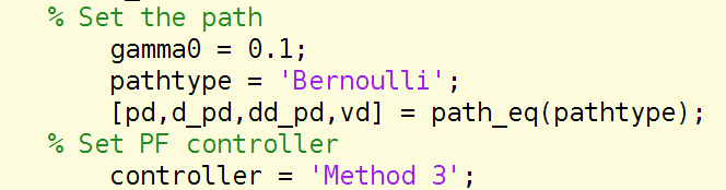
Figure 6.1: Path following toolbox main file: ’PFtool.m’

After running the “PFtool.m” file, the toolbox will animate and plot results as illustrated in Fig. 6.2. See also animation videos at https://youtu.be/XutfsXijHPE.

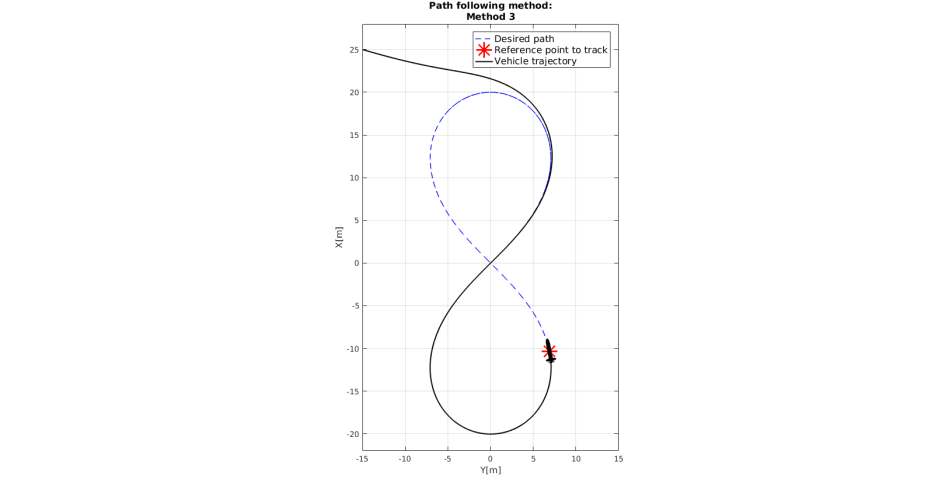
a) Example 1: Bernoulli path with Method 3
 

 
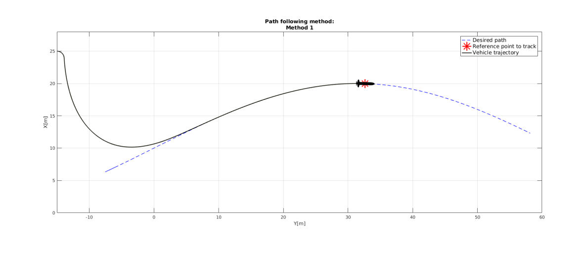
b) Example 2: Sinusoidal path with Method 1

Figure 6.2: Simulation example with different paths and path following methods

6.2 Gazebo/ROS packages

In order to test the path following algorithms with the Medusa vehicles in realistic a environment. We developed two efficient ROS packages in C++ that are used to run the algorithms on the on-board computers of the vehicles, namely i) a paths package for the generation of conveniently parameterized planar paths and ii) a path following algorithm package. These code libraries communicate with each other according to Fig. 6.3, using ROS topics. The paths library implements four simple parametric consisting of: arcs, lines, circles and Bernoulli lemniscates, as illustrated in Fig 6.4.

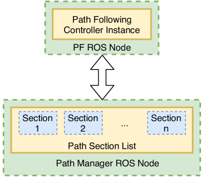
Figure 6.3: ROS node abstraction

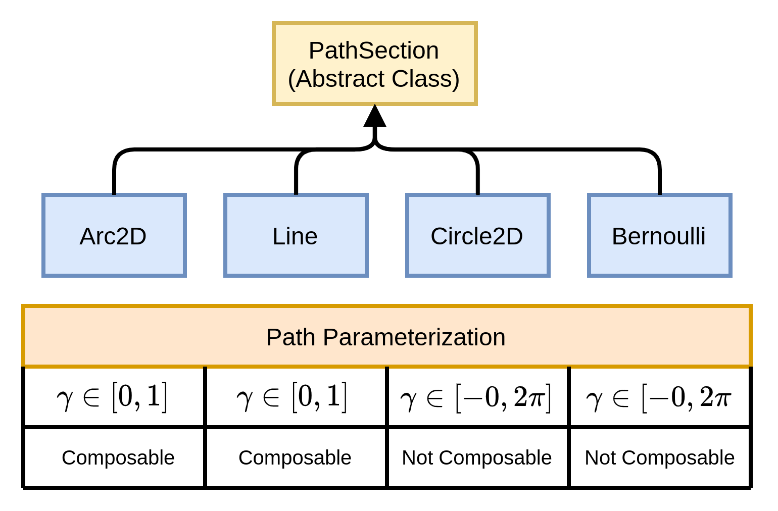
Figure 6.4: Paths Library

The paths library works as a state machine, such that multiple segments that are marked as “composable” can be added together to form more complex shapes. This flexible structure allows for the switching of the path following methods in use and the paths being followed in real time. The complete path following system implemented based on this structure is illustrated in Fig. 6.5.

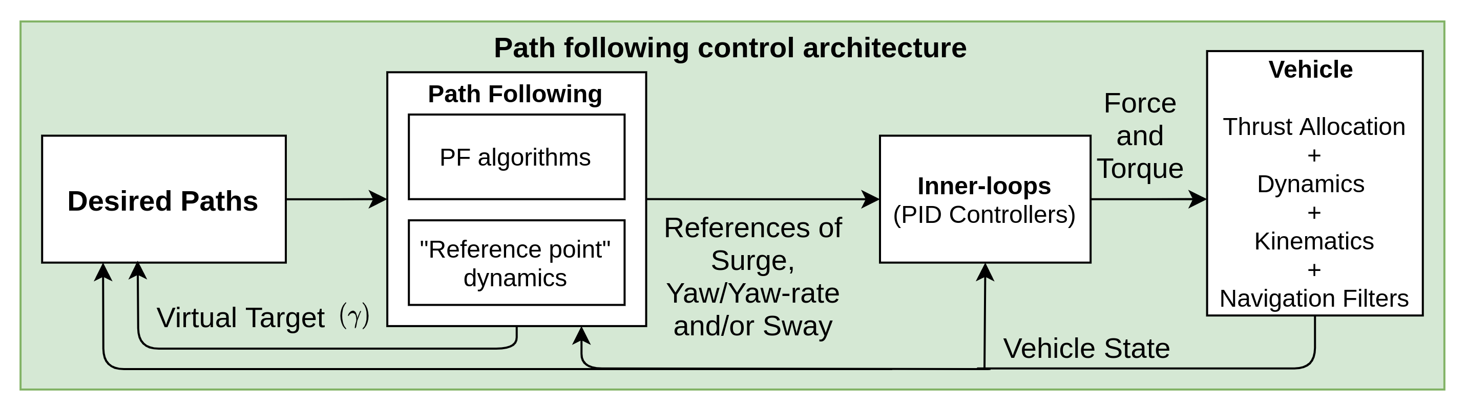
Figure 6.5: Complete path following control system implemented in Medusa vehicles

To allow the reader to perform experiments similar to the ones presented in this paper we provide in https://github.com/dsor-isr/Paper-PathFollowingSurvey a realistic simulation environment, resorting to the UUVSimulator Plugin and Gazebo 11 simulator [MSV⁺16], widely used in the robotics community. This makes it possible for the reader to simulate the real conditions found a the Olivais Dock at Parque das Nações, Lisbon, during field trials.

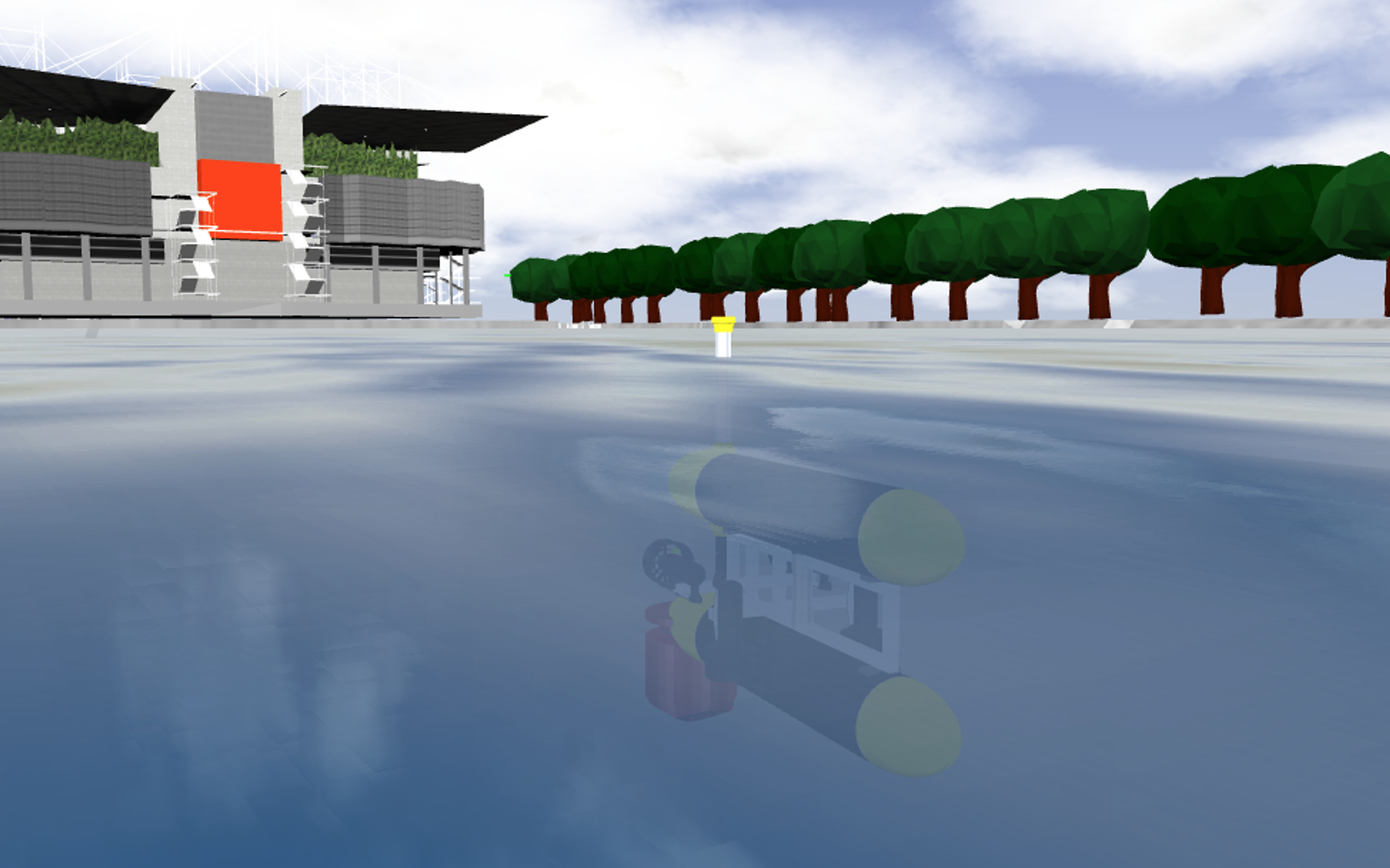
Figure 6.6: Medusa 3-D simulation using Gazebo

7 Simulation and experimental results

In this section, we start by introducing the test set-up adopted for conducting trials with the Medusa class of marine vehicles. Following suit, Hardware-in-the-Loop (HIL) simulation results obtained by resorting to Gazebo simulator are presented for the case of a an over-actuated Medusa vehicle, followed by real field trials results.

7.1 Test set-up

The field tests were conducted with two Medusa class autonomous surface vehicles built at IST. The first one is an under-actuated Medusa shown in Fig.2.4. This type of vehicle has played central roles in many European research projects such as Morph[CBB⁺15] and Wimust [AMP⁺16] to support the research in marine science and also in the area of guidance, navigation and control of single and networked multiple autonomous vehicle. The under-actuated Medusa vehicle is equipped with two thrusters located at starboard and portside that allow for the generation of longitudinal forces and torques about the vertical axis. The second Medusa that was used in the trial is over-actuated that is shown in Fig.2.5. This vehicle contain six thrusters. Two thrusters are mounted vertically and four thrusters are mounted horizontally. The thruster configuration in the over-actuated vehicle allows for the generation of longitudinal and lateral forces and torque about the vertical axis.
Each vehicle’s navigation system builds upon GPS-RTK and AHRS sensors that allow for the computation of its position and orientation. All software modules for navigation and control were implemented using the Robot Operating System (ROS, Melodic version), programmed with C++, and ran on an EPIC computer board (model NANO-PVD5251). More information about the specification of the Medusa class vehicle can be found in [ABG⁺16]. The implementation of the path following controllers follows the structure depicted in Fig. 2.2. The vehicle’s inner-loop controllers include four proportional integrator and derivative (PID)-type controllers to track the references in linear speed, heading, heading rate, and sway (only for over-actuated vehicles) that are generated by the path following controllers.
Snapshots showing the vehicle performing path following can be seen in Fig.7.1 while its operation can be monitored online with a console shown in 7.2.

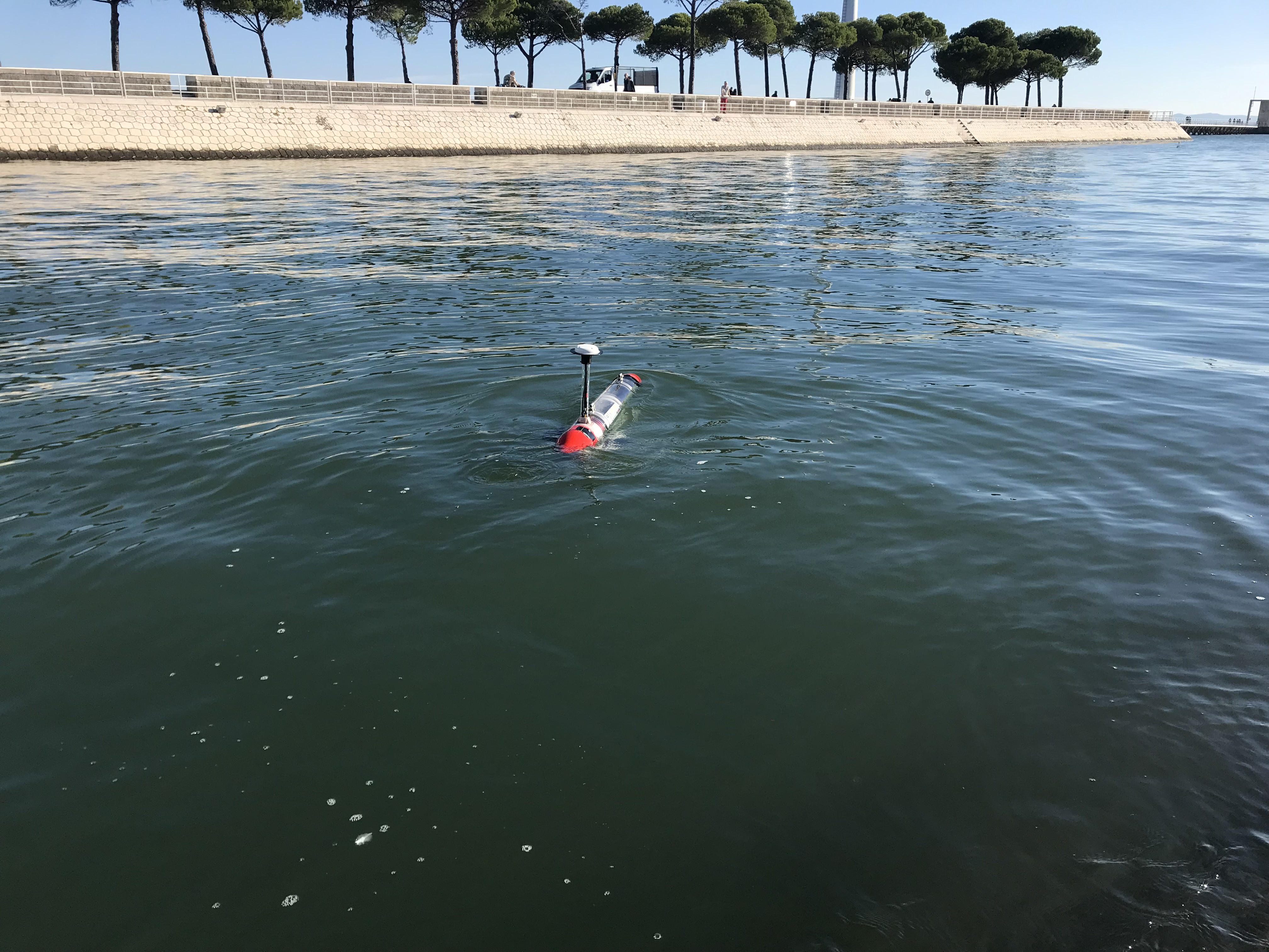
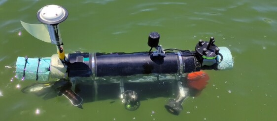
Figure 7.1: The Medusa vehicles performing path following during the trial. Left: under-actuated Medusa (a closer view can be seen in Fig. 2.4(a)), Right: over-actuated Medusa.

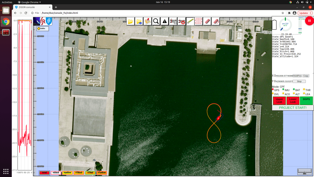
Figure 7.2: Console used to operate the Medusa class vehicles

7.2 Simulation results

Prior to operating any vehicle in a real world environment, it is common practice to resort to HIL simulations to analyse the performance of the controllers developed. In Figures 7.3 and 7.4 we can observe a lawn-mowing mission executed by an over-actuated Medusa vehicle, in the Gazebo simulator, using the path following method proposed in Section 5. In particular, Figure 7.3 shows the X-Y trajectory of the vehicle, that was requested to keep its yaw angle offset by $45^{\circ}$ from the tangent to the path.
Figure 7.3: Vehicle trajectory using the method described in Section 5. Figure 7.4: Cross-track and along-tracks errors and vehicle heading.  

In Figure 7.4 it can be observed that the along-track error converges to zero, while the cross-track and heading errors exhibit small static errors in the neighbourhood of zero. These errors result from the linear inner-loops implemented, a simplification in the design process which does not take into consideration the cross-terms in surge, sway and yaw in the dynamics of the vehicle.

7.3 Experimental results

7.3.1 Results with an under-actuated vehicle

This section describes the results of experimental tests whereby an under-actuated vehicle was requested to follow the same path repeatedly, using different path following algorithms. As shown in Fig. 7.5, during the tests the vehicle followed a lawnmowing path with a first leg of $30m$ heading east, then a half circumference turning clockwise with a radius of $10m$, a second leg of $20m$ heading west, another half circumference with a radius of $10m$ turning anticlockwise, and a final leg of $30m$ heading east. In another set of tests the vehicle was requested follow a Bernoulli lemniscate with a length of $20m$ as shown in 7.6. In all the tests, the assigned speed of the vehicles $U_{\rm d}$ is $0.5m/s$. The trials included the use of Method 1-4, 6, and the method in [MAP09].
Figures 7.5 and 7.6 show the paths of the vehicle during the trials, for the different methods. We observe that the vehicles follow their assigned paths and that the transient behavior and tracking performance vary according to the method used.

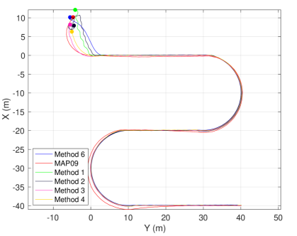
Figure 7.5: Vehicle’s paths using different path following methods to follow a lawnmower path in real trials. Filled circles are the positions of the vehicle at the beginning of each run.

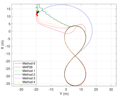
Figure 7.6: Vehicle’s paths using different path following methods to follow a Bernoulli lemniscate path in real trials. Filled circles are the positions of the vehicle at the beginning of each run.

The cross-track errors $y_{1}$ (defined in Section 3.2) of the vehicles performing a lawnmowing maneuver using different path following methods is shown in Figure 7.7. Identical results for the case where the path is a Bernoulli lemniscate are shown in 7.8.

Figure 7.7: Cross-track errors for different methods while performing lawnmower maneuvers.

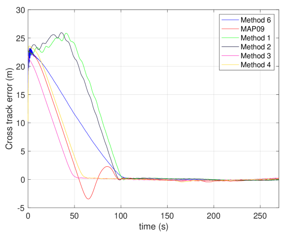
Figure 7.8: Cross-track errors for different methods while describing a Bernoulli lemniscate.

From Figures 7.7-7.8 one can observe that Methods 3-4 took less time to converge than the other methods.
The along-track errors $s_{1}$, defined in Section 3.2, of the vehicle performing a lawnmowing maneuver and following a Bernoulli lemniscate are shown in Fig. 7.9 and Fig. 7.10, respectively. Figures 7.9-7.10 show the data for Method 2, 4 and 6 since for all the other methods the “reference point” is the orthogonal projection of the vehicle’s position on the path which makes the along-track error equals to zero.

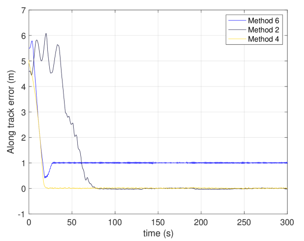
Figure 7.9: Along-track errors for different methods while performing lawn-mowing maneuvers.

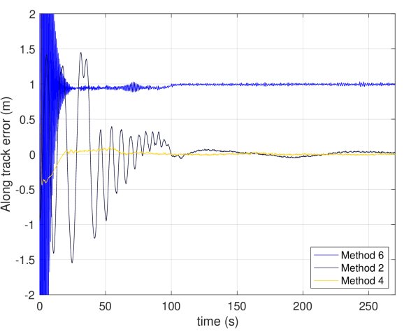
Figure 7.10: Along-track errors for different methods while describing a Bernoulli lemniscate.

From Figures 7.9-7.10 one can observe that the along track error converges to close to zero for Method 2 and 4 and for Method 6 stabilizes at $1m$ due to the effect of $\boldsymbol{\epsilon}$ on the particular definition of the position error, see (46). We can also observe, for the Bernoulli lemniscate mission with Method 6, large oscillations at the beginning.
Figures 7.11 and 7.12 show the surge speed $u$ of the vehicle for different methods for the lawnmower and Bernoulli lemniscate missions respectively, which clearly indicate that the vehicle asymptotically reaches the desired constant speed profile (0.5m/s). However they show that the surge speed converged faster to the desired speed for Method 3, 4 and the Method in [MAP09].

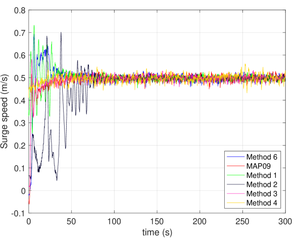
Figure 7.11: Surge speed for different methods while performing lawnmower maneuvers.

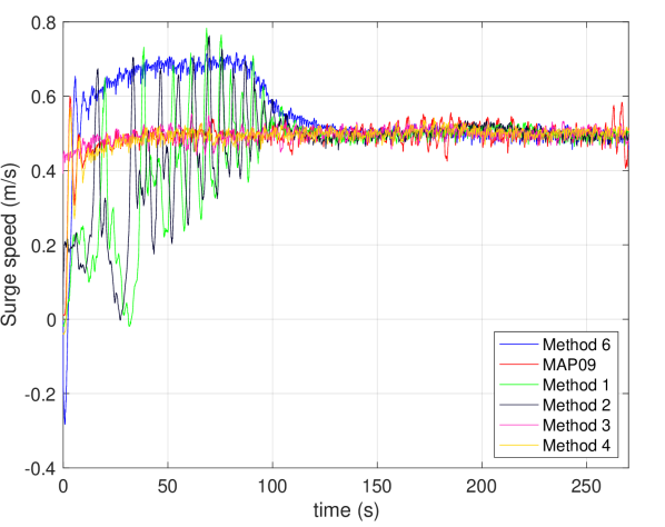
Figure 7.12: Surge speed for different methods while describing a Bernoulli lemniscate.

7.3.2 Results with an over-actuated vehicle

The method for over-actuated vehicles described in Section 5 was tested with a over-actuated Medusa class vehicle following a line due east (along the $Y$ axis) with a heading $\psi$ of $0^{\circ}$. The obtained path, along and cross track erros, and yaw are shown in Figures 7.13, 7.14 and 7.15, respectively.

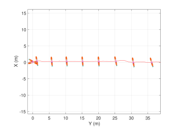
Figure 7.13: Vehicle path using the method described in Section 5. The initial positions of the vehicle is (0,0).

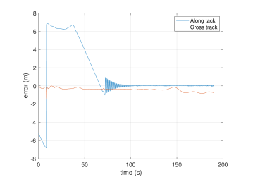
Figure 7.14: Along and cross track errors during the mission of Figure 7.13.

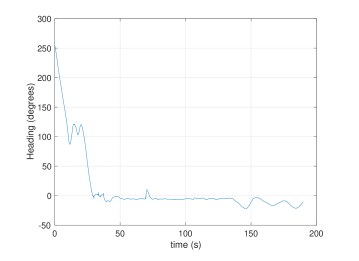
Figure 7.15: Yaw during the mission of Figure 7.13.

Given the coupling between surge, sway and yaw rate in the dynamics of the vehicle, the tunning of the PID inner loops of the real vehicle is a challenging task and we were not able to obtain adequate performance of circular maneuvers during the field trials with simple linear control laws. From Fig. 7.14 one can observe that the along-track error starts at around $5m$ because that is the distance from the initial position of the vehicle to the beginning of the path, but one can observe that the vehicle converges to the beginning of the path in around $70s$. Also one can observe that the cross-track error remains below $1m$ during the mission. Finally, from Fig. 7.15 the heading converges to within $15^{\circ}$ of the reference. Future work will involve the design of new nonlinear inner loop controllers to achieve better performance.

8 Discussions

8.1 Advantages and disadvantages of the different path following methods

In this section we discuss some of the benefits and drawbacks of the path following methods reviewed in the previous sections and compare them with other methods in the literature such as the vector field (VF) method described in [NBMB07]. A relative comparison in terms of complexity and flexibility is shown in Fig.8.1.
From an implementation standpoint, Methods 2,4, and 6 are the simplest and can therefore be considered as good candidates to solve path following problems. These methods are elegant in the sense that the “reference point” on the path that the vehicle must track in order to achieve path following is not necessary the closest to the vehicle. Instead, it can be initialized anywhere on the path, after which its evolution is controlled via $\dot{\gamma}$ or $\ddot{\gamma}$ to attract the vehicle to the path and make it follow that path with a desired speed. Among these methods, Method 4 is the simplest while Method 2 is the more complicated since it requires to know the knowledge of path’s curvature. However, it can be expected that for time varying curvature paths, Method 2 will outperform Method 4.
Methods 1 and 3, on the other hand, are more complex in general, as they consider “reference point” the one closest to the vehicle which, in the case of general paths requires solving an optimization on-line to find this point. Comparing the two methods, it can be said that Method 1 is more complicated as it requires to know the function of curvature along the path; however, one might expect that it outperforms Method 3 for paths with varying curvature.
VF methods are more flexible than those discussed above in the sense that they can be extended to deal with the problem of obstacle avoidance [WC19]. However, they are more complex in terms of derivation and proof of stability.
Methods 5 and 7 (NMPC-based approaches) are the most complicated, in terms of design and implementation, since they involve solving an optimization problem online that is non-convex, due to the kinematic constraints of the vehicles. However, these methods deal with the vehicle’s input constraints (eg. velocity and angular rate) explicitly, an important feature that none of the methods mentioned before has. For this reason, NMPC based-approaches are expected to outperform the others in path following missions that require the vehicle to maneuver more aggressively, pushing the actuation values close to their limits. Another advantage of NMPC-based methods is that they can incorporate easily other tasks such as obstacle avoidance in the path following problem [SSNS18].

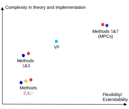
Figure 8.1: A comparison among the path following methods.

8.2 Other issues

As explained before, the main focus of this paper is on path following methods that can be designed by taking into consideration the vehicle kinematics only. It is tacitly assumed that inner control loops can be implemented to make the vehicle´s relevant variables track with good accuracy the commands issued by the outer path following control loop (e.g. speed, heading, heading rate, etc). This design approach is widely adopted by control practitioners because it simplifies considerably the design, analysis, and implementation steps. Experimental results reported in the literature, see for example [TMD⁺07, RHJ⁺19, BBCL09] and the results presented in Section 7, suggest that this should be the first candidate approach to solve path following control problems. From a theoretical standpoint, however it is generally not trivial to guarantee that the path following methods developed at the kinematic level also preserve adequate performance with non-ideal tracking inner-loop controllers. With Method 6, the conclusion is in the affirmative as reported in [RHJ⁺19, Van07, MAP09], where it is shown that the complete path following error system is ISS with respect to the tracking errors associated with speed and yaw-rate tracking controllers. This implies that as long as the tracking errors are bounded then the path following error is bounded. Relate results can be found in [KPX⁺17]. A similar property may very well hold with the other path following methods summarized in this paper; however, proofs for these methods are not available in the literature.
Another issue with the inner-outer loop approach is that it requires the inner-loop controllers to be fine tuned to guarantee that the complete path following system is stable and and achieves a desired degree of performance; the tuning process can be time-consuming and in many cases it is also expensive. In order to deal with this problem, the work in [KPX⁺10] suggests augmenting the inner-loop controllers with “Ł1 adaptive controllers”, that aim at eliminating the effect of inner-loop uncertainty on the total path following system. See [MCC15, XOG21] for applications of this strategy to an underwater robot and a surface ship, respectively.
Another type of path following methods involves including explicitly the vehicle dynamics in the design process. A typical example of this approach can be found in[LSP06, AH07] where the authors employ backstepping technique sto derive control laws for the vehicle force and toque to achieve path following. The main challenge of this approach is that it is harder to design as the vehicle model adopted for controller design is far more complex than the kinematic model. In addition, the dynamics of the vehicle normally exhibit large uncertainty in the parameters (e.g. mass, momentums of inertia, hydrodynamic or aerodynamic drag terms, etc.) thus making the design process quite challenging.
Finally, there is also a considerable interest in using learning-based methods for the path following problem in recent years. These type of method aims at dealing with vehicles model and environment uncertainty. Along this line, learning-based MPC methods suggested in [OSBC16, RMNM20] seem to be a promising approach while reinforcement learning-based methods described in [ML18, KZL19, WDWR21] are also worth considering. Although these methods are powerful, they are far complicated than the methods derived in Section 3. Furthermore these methods lack of stability guarantee and for RL-based methods, they lack of intuition underlying the controller and thus make it difficult to tune.

9 Conclusions

Path following of autonomous robotic vehicles is a fairly well understood and established technique for kinematic vehicle models, and a variety of solutions to the path following problem have been published in the literature. Motivated by the need to bring many of the methods under a common umbrella, this paper presented an in-depth review of the topic of path following for autonomous vehicle moving in 2D, showing clearly how many of the existing techniques can be derived under a unified mathematical framework that makes use of nonlinear control theory. The paper provided a rigorous analysis of the main classes of methodologies identified and discussed the advantages and disadvantages of each method, comparing them from a design and implementation standpoint. In addition, the paper described the steps involved in going from theory to practice through the introduction of Matlab and Gazebo/ROS simulation toolboxes that are helpful in testing path following methods prior to their integration in the combined guidance, navigation, and control systems of autonomous vehicles. Finally, the paper discussed the results of experimental field tests with underactuated and overactuated autonomous marine vehicles performing path following maneuvers.
The simulations and experimental results showed that as long as the inner-loop /dynamic) tracking controllers for speed, heading, or heading rate issued by the (outer loop/kinematic ) path following controller are well tuned and there is adequate time scale separation of the inner and outer loops systems, the methods exposed in the paper for kinematic models hold very good potential for real life applications.
For missions involving vehicles for which the inner and outer loop dynamics do not exhibit a clear two scale separation and yet require good path following performance, methods that take explicitly into account the vehicle dynamics in the design of path following strategies may be required. Considerable research has been done in this area, but to the space limitations this survey did not address them. See [LSP06] for a representative early example that resorts to backstepping and vehicle parameter adaptation strategies. The example shows clearly how the explicit intertwining of kinematics and dynamics in path following control system design complicates the design process, yields controllers with increased complexity that may be difficult to implement, and requires knowledge of the vehicle´s parameters (such as hydrodynamic or aerodynamic terms) and its actuators, which normally exhibit high degrees of uncertainty. A trending approach to deal with uncertainty in vehicle and actuator models is to use learning based techniques such as learning-MPC or reinforcement learning for path following. However, existing methods lack formal stability guarantees and fail to capture physically-based intuition that is often crucial in the design and tuning of advanced control systems. Clearly, further research is required to ascertain if such methods can be further developed to obtain proven performance guarantees, a significant step required to make a control systems applicable in practice.

Disclosure statement

The authors confirm that there are no known conflicts of interest associated with this publication.

10 Appendix

10.1 Basic results

The following lemma was used in the paper.

Lemma 10.1 (Rotation Matrix Differential Equation, Theorem 2.2 [Fos11]).

Let $R^{B}_{A}\in SO(n)$$(n=2,3)$ be the rotation matrix from frame $\{A\}$ to frame $\{B\}$. Then,

$$\dot{R}^{B}_{A}={R}^{B}_{A}S(\boldsymbol{\omega}^{A}_{A/B}),$$ (79)

where $S(\boldsymbol{\omega}^{A}_{A/B})$ is a Skew-symmetric matrix and $\boldsymbol{\omega}^{A}_{A/B}\in\mathbb{R}^{n}$ is the angular velocity vector of $\{A\}$ respect to $\{B\}$, expressed in $\{A\}$.

10.2 Proofs

10.2.1 Proof of Theorem 3.1

Consider the Lyapunov function candidate $V_{1}$ defined by

$$V_{1}=\frac{1}{2}y^{2}_{1}+\frac{1}{2k_{2}}\tilde{\psi}^{2}$$ (80)

Taking its time derivative yields

$$\dot{V}_{1}=y_{1}\dot{y}_{1}+\frac{1}{k_{2}}\tilde{\psi}\dot{\tilde{\psi}}\stackrel{{\scriptstyle\eqref{eq: y1dot},\eqref{eq: dot_tilde_psi},\eqref{eq: r samson}}}{{=}}y_{1}u\sin\delta-\frac{k_{1}}{k_{2}}\tilde{\psi}^{2}.$$ (81)

Because of Condition 1, $\dot{V}_{1}\leq 0$ for all $t$. Furthermore, the above equation shows that $\dot{V}_{1}$ is uniform continuous and therefore, using Barbalat’s Lemma [Has02], we conclude that $\dot{V}_{1}(t)$ converges to zero as $t\to\infty$. In view of (81) and Condition 1, this implies that $y_{1}(t),\tilde{\psi}(t)\to 0$ as $t\to\infty$. $\blacksquare$

10.2.2 Proof of Theorem 3.2

The proof can be done by employing the Lyapunov function candidate given by

$$V_{2}=\frac{1}{2}{\bf e}_{\scriptscriptstyle{\mathcal{P}}}^{2}+\frac{1}{2k_{2}}\tilde{\psi}^{2}.$$ (82)

Taking its time derivative yields

$$\dot{V}_{2}={\bf e}_{\scriptscriptstyle{\mathcal{P}}}^{\top}\dot{{\bf e}}_{\scriptscriptstyle{\mathcal{P}}}-\frac{1}{k_{2}}\tilde{\psi}\dot{\tilde{\psi}}\stackrel{{\scriptstyle\eqref{eq: dot eP},\eqref{eq: dot_tilde_psi}}}{{=}}{\bf e}_{\scriptscriptstyle{\mathcal{P}}}^{\top}\begin{bmatrix}u\cos(\psi_{\rm e})-u_{\scriptscriptstyle{\mathcal{P}}}\\ u\sin(\psi_{\rm e})\end{bmatrix}+\frac{1}{k_{2}}\tilde{\psi}(r-\kappa(\gamma)u_{\scriptscriptstyle{\mathcal{P}}}-\dot{\delta}).$$ (83)

In the above, we have used the fact that for any Skew-symmetric matrix $S$, ${\bf x}^{\top}S{\bf x}=0$ for all ${\bf x}$, thus ${\bf e}_{\scriptscriptstyle{\mathcal{P}}}^{\top}S(\boldsymbol{\omega}_{\scriptscriptstyle{\mathcal{P}}}){\bf e}_{\scriptscriptstyle{\mathcal{P}}}=0$. Substituting $r$ given by (30) and $u_{\scriptscriptstyle{\mathcal{P}}}$ given by (33) in $\dot{V}_{2}$, we obtain

$$\dot{V}_{2}=-k_{3}s^{2}_{1}+y_{1}u\sin\delta-\frac{k_{1}}{k_{2}}\tilde{\psi}^{2}.$$ (84)

Due to Condition 1, we conclude that $\dot{V}_{2}\leq 0$ for all $t$. Furthermore, the above equation shows that $\dot{V}_{2}$ is uniform continuous; thus, invoking Barbalat’s lemma [Has02], $\dot{V}_{2}(t)$ converges to 0 as $t\to\infty$. In view of (84) this implies that $s_{1}(t),y_{1}(t),\tilde{\psi}(t)\to 0$ as $t\to\infty$. Notice that because of Condition 1 once $y_{1},\tilde{\psi}\to 0$, $\psi_{e}\to 0$ as well. $\blacksquare$

10.2.3 Proof of Theorem 3.3

Consider the Lyapunov function candidate $V_{3}$, given by $V_{3}=y^{2}_{1}/2$. Taking its time derivative yields

$$\dot{V}_{3}=y_{1}\dot{y}_{1}\stackrel{{\scriptstyle\eqref{eq: y1dot},\eqref{eq: psie in PF method 3}}}{{=}}-u\frac{y^{2}_{1}}{\sqrt{y^{2}_{1}+\Delta^{2}_{\rm h}}}\stackrel{{\scriptstyle\eqref{eq: u samson}}}{{=}}-U_{\rm d}\frac{y^{2}_{1}}{\sqrt{y^{2}_{1}+\Delta^{2}_{\rm h}}}$$

Since $U_{\rm d}$ (the desired speed profile for the vehicle to track) is always positive, $\dot{V}_{3}\leq 0$ for all $y_{1}$. It can be seen that $\dot{V}_{3}$ is uniform continuous, and therefore invoking Barbalat’s lemma [Has02] $\dot{V}_{3}(t)$ converges to 0 as $t\to\infty$. This implies that $y_{1}(t)$ converges to zero as $t\to\infty$. $\blacksquare$

10.2.4 Proof of Theorem 3.4

First, substituting $u_{\scriptscriptstyle{\mathcal{P}}}$ given by (33) and $\psi_{\rm e}$ given by (35) in (23) yields the dynamics of the position error in the resulting closed-loop system as

$$\dot{{\bf e}}_{\scriptscriptstyle{\mathcal{P}}}=-S(\boldsymbol{\omega}_{\scriptscriptstyle{\mathcal{P}}}){\bf e}_{\scriptscriptstyle{\mathcal{P}}}-\begin{bmatrix}-k_{3}s_{1}\\ -uy_{1}/\sqrt{y^{2}_{1}+\Delta^{2}_{\rm h}}\end{bmatrix}.$$ (85)

Consider the Lyapunov function candidate, given by $V_{4}({\bf e}_{\scriptscriptstyle{\mathcal{P}}})=\frac{1}{2}{\bf e}^{\top}_{\scriptscriptstyle{\mathcal{P}}}{\bf e}_{\scriptscriptstyle{\mathcal{P}}}$. Taking its time derivative yields

$$\dot{V}_{4}={\bf e}^{\top}_{\scriptscriptstyle{\mathcal{P}}}\dot{{\bf e}}_{\scriptscriptstyle{\mathcal{P}}}\stackrel{{\scriptstyle\eqref{eq: doteP closed loop method 3}}}{{=}}-k_{3}s^{2}_{1}-u\frac{y^{2}_{1}}{\sqrt{y^{2}_{1}+\Delta^{2}_{\rm h}}}\stackrel{{\scriptstyle\eqref{eq: u samson}}}{{=}}-k_{3}s^{2}_{1}-U_{\rm d}\frac{y^{2}_{1}}{\sqrt{y^{2}_{1}+\Delta^{2}_{\rm h}}}.$$ (86)

Note that we used the fact that ${\bf e}^{\top}_{\scriptscriptstyle{\mathcal{P}}}S(\boldsymbol{\omega}_{\scriptscriptstyle{\mathcal{P}}}){\bf e}_{\scriptscriptstyle{\mathcal{P}}}=0$ for all ${\bf e}_{\scriptscriptstyle{\mathcal{P}}}$ because $S$ is a Skew-symmetric matrix. Furthermore, because $u=U_{\rm d}$, which is always positive, we conclude that $\dot{V}_{4}<0$ for ${\bf e}_{\scriptscriptstyle{\mathcal{P}}}$. Since $u$ is in general a function of time then the closed-loop position error system (85) is non-autonomous, therefore we conclude that the origin of ${\bf e}_{\scriptscriptstyle{\mathcal{P}}}$ is UGAS. $\blacksquare$

10.2.5 Proof of Theorem 3.6

Consider a Lyapunov function candidate for the path following system (51), given by

$$V_{6}({\bf x})=\frac{1}{2}{\left\|{\bf x}\right\|}^{2}=\frac{1}{2}{\bf e}^{\top}_{\scriptscriptstyle{\mathcal{B}}}{\bf e}_{\scriptscriptstyle{\mathcal{B}}}+\frac{1}{2}e^{2}_{\gamma}.$$ (87)

Taking its time derivative yields

$$\begin{split}\dot{V}_{6}&={\bf e}^{\top}_{\scriptscriptstyle{\mathcal{B}}}\dot{{\bf e}}_{\scriptscriptstyle{\mathcal{B}}}+e_{\gamma}\dot{e}_{\gamma}\\ &\stackrel{{\scriptstyle\eqref{eq: following error aguiar method},\eqref{eq: gamma dot}}}{{=}}{\bf e}^{\top}_{\scriptscriptstyle{\mathcal{B}}}\left(−S(\boldsymbol{\omega}){{\bf e}}_{\scriptscriptstyle{\mathcal{B}}}+\Delta{\bf u}−R^{\scriptscriptstyle{\mathcal{B}}}_{\scriptscriptstyle{\mathcal{I}}}(\psi){\bf p}^{\prime}_{\rm d}(\gamma)\dot{\gamma}\right)+e_{\gamma}\left(\ddot{\gamma}-\dot{v}_{\rm d}\right).\\ &\stackrel{{\scriptstyle\eqref{eq: Aguiar controller},\eqref{eq: e gamma}}}{{=}}-{\bf e}_{\scriptscriptstyle{\mathcal{B}}}^{\top}K_{\rm p}{\bf e}_{\scriptscriptstyle{\mathcal{B}}}-k_{\gamma}e^{2}_{\gamma}.\end{split}$$ (88)

Let $K={\rm diag}(K_{\rm p},k_{\gamma})$, then $\dot{V}_{6}=-{\bf x}^{\top}K{\bf x}\leq-\lambda_{\min}(K){\left\|{\bf x}\right\|}^{2}$ for all ${\bf x}\neq\boldsymbol{0}$. Thus, we conclude that the origin of $\bf x$ is GES. $\blacksquare$

10.2.6 Proof of Lemma 4.4

Consider again the Lyapunov function candidate $V_{6}$ given by (90). Substituting ${\bf u}$ in (74) and $\ddot{\gamma}$ in (52b) in (73) and (50) yields

$$\begin{split}\dot{V}_{6}&={\bf e}^{\top}_{\scriptscriptstyle{\mathcal{B}}}\dot{{\bf e}}_{\scriptscriptstyle{\mathcal{B}}}+e_{\gamma}\dot{e}_{\gamma}\\ &=-{\bf e}_{\scriptscriptstyle{\mathcal{B}}}^{\top}K_{\rm p}{\bf e}_{\scriptscriptstyle{\mathcal{B}}}-k_{\gamma}e^{2}_{\gamma}-{\bf e}_{\scriptscriptstyle{\mathcal{B}}}^{\top}R^{\scriptscriptstyle{\mathcal{B}}}_{\scriptscriptstyle{\mathcal{I}}}(\psi){\bf e}_{c}\\ &\leq-\lambda_{\rm min}(K){\left\|{{\bf x}}\right\|}^{2}+{\left\|{{\bf x}}\right\|}{\left\|{{\bf e}_{c}}\right\|}\end{split}$$ (89)

Thus, invoking Theorem 4.19 in [Has02] we conclude that the path following error system is ISS respect to the input ${\bf e}_{c}$. $\blacksquare$

10.2.7 Proof of Theorem 5.1

Consider a Lyapunov function candidate for the path following system (77), given by

$$V_{F}({\bf x})=\frac{1}{2}{\left\|{\bf x}\right\|}^{2}=\frac{1}{2}{\bf e}^{\rm T}_{\scriptscriptstyle{\mathcal{B}}}{\bf e}_{\scriptscriptstyle{\mathcal{B}}}+\frac{1}{2}e^{2}_{\gamma}.$$ (90)

Taking its time derivative yields

$$\begin{split}\dot{V}_{F}&={\bf e}^{\rm T}_{\scriptscriptstyle{\mathcal{B}}}\dot{{\bf e}}_{\scriptscriptstyle{\mathcal{B}}}+e_{\gamma}\dot{e}_{\gamma}\\ &\stackrel{{\scriptstyle\eqref{eq: following error aguiar method},\eqref{eq: gamma dot}}}{{=}}{\bf e}^{\rm T}_{\scriptscriptstyle{\mathcal{B}}}\left(−S(\boldsymbol{\omega}){{\bf e}}_{\scriptscriptstyle{\mathcal{B}}}+{\bf v}−R^{\scriptscriptstyle{\mathcal{B}}}_{\scriptscriptstyle{\mathcal{I}}}(\psi){\bf p}^{\prime}_{\rm d}(\gamma)\dot{\gamma}\right)+e_{\gamma}\left(\ddot{\gamma}-\dot{v}_{\rm d}\right).\\ &\stackrel{{\scriptstyle\eqref{eq: fully actuated controller},\eqref{eq: e gamma}}}{{=}}-{\bf e}_{\scriptscriptstyle{\mathcal{B}}}^{\rm T}K_{\rm p}{\bf e}_{\scriptscriptstyle{\mathcal{B}}}-k_{\gamma}e^{2}_{\gamma}.\end{split}$$ (91)

Let $K={\rm diag}(K_{\rm p},k_{\gamma})$, then $\dot{V}_{F}=-{\bf x}^{\rm T}K{\bf x}\leq-\lambda_{\min}(K){\left\|{\bf x}\right\|}^{2}$ for all ${\bf x}\neq\boldsymbol{0}$. Thus, we conclude that the origin of $\bf x$ is GES. $\blacksquare$

References

- [AAJ13] Andrea Alessandretti, A Pedro Aguiar, and Colin N Jones. Trajectory-tracking and path-following controllers for constrained underactuated vehicles using model predictive control. In Control Conference (ECC), 2013 European, pages 1371–1376. IEEE, 2013.
- [ABG+16] Pedro Caldeira Abreu, João Botelho, Pedro Góis, Antonio Pascoal, Jorge Ribeiro, Miguel Ribeiro, Manuel Rufino, Luís Sebastião, and Henrique Silva. The medusa class of autonomous marine vehicles and their role in eu projects. In OCEANS 2016, pages 1–10. IEEE, 2016.
- [AGH+19] Joel A E Andersson, Joris Gillis, Greg Horn, James B Rawlings, and Moritz Diehl. CasADi – A software framework for nonlinear optimization and optimal control. Mathematical Programming Computation, 11(1):1–36, 2019.
- [AH07] A Pedro Aguiar and Joao P Hespanha. Trajectory-tracking and path-following of underactuated autonomous vehicles with parametric modeling uncertainty. IEEE Transactions on Automatic Control, 52(8):1362–1379, 2007.
- [AML13] Anastasios M. Lekkas Anastasios M. Lekkas. Advanced in Marine Robotics, chapter 5. Lambert Academic Publishing, 2013.
- [AMP+16] Pedro Abreu, Hélio Morishita, António Pascoal, Jorge Ribeiro, and Henrique Silva. Marine vehicles with streamers for geotechnical surveys: Modeling, positioning, and control**this research was supported by the ec wimust project (grant no. 645141) and the portuguese fct funding program [pest-oe/eei/la0009/2011]. the second author was supported by the brasilian navy during his sabbatical leave at the isr/ist, lisbon, portugal. IFAC-PapersOnLine, 49(23):458–464, 2016. 10th IFAC Conference on Control Applications in Marine SystemsCAMS 2016.
- [AOO+06] J. Alves, P. Oliveira, R. Oliveira, A. Pascoal, M. Rufino, L. Sebastiao, and C. Silvestre. Vehicle and mission control of the delfim autonomous surface craft. In 2006 14th Mediterranean Conference on Control and Automation, pages 1–6, 2006.
- [AP02] A.P. Aguiar and A.M. Pascoal. Dynamic positioning and way-point tracking of underactuated auvs in the presence of ocean currents. In Proceedings of the 41st IEEE Conference on Decision and Control, 2002., volume 2, pages 2105–2110 vol.2, 2002.
- [AWN12] Adeel Akhtar, Steven L Waslander, and Christopher Nielsen. Path following for a quadrotor using dynamic extension and transverse feedback linearization. In 2012 IEEE 51st IEEE Conference on Decision and Control (CDC), pages 3551–3556. IEEE, 2012.
- [BBCL09] Marco Bibuli, Gabriele Bruzzone, Massimo Caccia, and Lionel Lapierre. Path-following algorithms and experiments for an unmanned surface vehicle. Journal of Field Robotics, 26(8), 2009.
- [BF05] M. Breivik and T. I. Fossen. Principles of guidance-based path following in 2d and 3d. In Proceedings of the 44th IEEE Conference on Decision and Control, pages 627–634, 2005.
- [BZAF19] Ivo Batkovic, Mario Zanon, Mohammad Ali, and Paolo Falcone. Real-time constrained trajectory planning and vehicle control for proactive autonomous driving with road users. In 2019 18th European Control Conference (ECC), pages 256–262, 2019.
- [CBB+15] P. Caldeira Abreu, M. Bayat, J. Botelho, P. Góis, J. Gomes, A. Pascoal, J. Ribeiro, M. Ribeiro, M. Rufino, L. Sebastião, and H. Silva. Cooperative formation control in the scope of the ec morph project: Theory and experiments. In OCEANS 2015 - Genova, pages 1–7, 2015.
- [CPB+16] W. Caharija, K. Y. Pettersen, M. Bibuli, P. Calado, E. Zereik, J. Braga, J. T. Gravdahl, A. J. Sørensen, M. Milovanović, and G. Bruzzone. Integral line-of-sight guidance and control of underactuated marine vehicles: Theory, simulations, and experiments. IEEE Transactions on Control Systems Technology, 24(5):1623–1642, 2016.
- [DLOS98] Alessandro De Luca, Giuseppe Oriolo, and Claude Samson. Feedback control of a nonholonomic car-like robot. Robot motion planning and control, pages 171–253, 1998.
- [DOO03] O.H. Dagci, U.Y. Ogras, and U. Ozguner. Path following controller design using sliding mode control theory. In Proceedings of the 2003 American Control Conference, 2003., volume 1, pages 903–908 vol.1, 2003.
- [EP00] P. Encarnacao and A. Pascoal. 3d path following for autonomous underwater vehicle. In Proceedings of the 39th IEEE Conference on Decision and Control (Cat. No.00CH37187), volume 3, pages 2977–2982 vol.3, 2000.
- [FBS03] Thor I. Fossen, Morten Breivik, and Roger Skjetne. Line-of-sight path following of underactuated marine craft. IFAC Proceedings Volumes, 36(21):211 – 216, 2003. 6th IFAC Conference on Manoeuvring and Control of Marine Craft (MCMC 2003), Girona, Spain, 17-19 September, 1997.
- [FBT97] D. Fox, W. Burgard, and S. Thrun. The dynamic window approach to collision avoidance. IEEE Robotics Automation Magazine, 4(1):23–33, 1997.
- [FJP09] Thor I. Fossen, Tor Arne Johansen, and Tristan Perez. A survey of control allocation methods for underwater vehicles. In Alexander V. Inzartsev, editor, Underwater Vehicles, chapter 7. IntechOpen, Rijeka, 2009.
- [Fos11] Thor I Fossen. Handbook of marine craft hydrodynamics and motion control. John Wiley & Sons, 2011.
- [FPG15] T. I. Fossen, K. Y. Pettersen, and R. Galeazzi. Line-of-sight path following for dubins paths with adaptive sideslip compensation of drift forces. IEEE Transactions on Control Systems Technology, 23(2):820–827, 2015.
- [GAS06] Alfred Gray, Elsa Abbena, and Simon Salamon. Modern differential geometry of curves and surfaces with Mathematica®. third edition, 2006.
- [GCC+19] Hongyan Guo, Dongpu Cao, Hong Chen, Zhenping Sun, and Yunfeng Hu. Model predictive path following control for autonomous cars considering a measurable disturbance: Implementation, testing, and verification. Mechanical Systems and Signal Processing, 118:41–60, 2019.
- [Gho17] M.T. Ghorbani. Some notes on trajectory tracking and path following control of marine vehicles. IST Technical Report, 2017.
- [Gho21] M.T. Ghorbani. A wall-following controller design method for underactuated auvs: An adaptive internal model approach. IFAC-PapersOnLine, 54(16):314–319, 2021. 13th IFAC Conference on Control Applications in Marine Systems, Robotics, and Vehicles CAMS 2021.
- [Has02] Khalil Hassan. Nonlinear systems. Prentice Hall, New Jewsey, 3rd edition, 2002.
- [HCC+04] Daniel M Helmick, Yang Cheng, Daniel S Clouse, Larry H Matthies, and Stergios I Roumeliotis. Path following using visual odometry for a mars rover in high-slip environments. In 2004 IEEE Aerospace Conference Proceedings (IEEE Cat. No. 04TH8720), volume 2, pages 772–789. IEEE, 2004.
- [HFD11] B. Houska, H.J. Ferreau, and M. Diehl. ACADO Toolkit – An Open Source Framework for Automatic Control and Dynamic Optimization. Optimal Control Applications and Methods, 32(3):298–312, 2011.
- [HM95] Andrew J. Hanson and Hui Ma. Parallel transport approach to curve framing. Technical report, 1995.
- [HPJ20] Nguyen T. Hung, Antonio M. Pascoal, and Tor A. Johansen. Cooperative path following of constrained autonomous vehicles with model predictive control and event triggered communications. International Journal of Robust and Nonlinear Control, 2020.
- [HRCP18] N. T. Hung, F. Rego, N. Crasta, and A.M. Pascoal. Input-constrained path following for autonomous marine vehicles with a global region of attraction. In 11th IFAC Conference on Control Applications in Marine Systems, Robotics, and Vehicles CAMS 2018, volume 51, pages 348 – 353, 2018.
- [Jac21] Marcelo Fialho Jacinto. Cooperative motion control of aerial and marine vehicles for environmental applications. Master’s thesis, Instituto Superior Tecnico, Av. Rovisco Pais 1, 1049-001 Lisboa, 2021. https://fenix.tecnico.ulisboa.pt/cursos/meec/dissertacao/1972678479054971.
- [JF13] Tor A. Johansen and Thor I. Fossen. Control allocation—a survey. Automatica, 49(5):1087–1103, 2013.
- [JH05] A. Jadbabaie and J. Hauser. On the stability of receding horizon control with a general terminal cost. IEEE Transactions on Automatic Control, 50(5):674–678, 2005.
- [KPX+10] Isaac Kaminer, Antonio Pascoal, Enric Xargay, Naira Hovakimyan, Chengyu Cao, and Vladimir Dobrokhodov. Path following for small unmanned aerial vehicles using l1 adaptive augmentation of commercial autopilots. Journal of Guidance, Control, and Dynamics, 33(2):550–564, 2010.
- [KPX+17] Isaac Kaminer, António Pascoal, Enric Xargay, Naira Hovakimyan, Venanzio Cichella, and Vladimir Dobrokhodov. Time-Critical Cooperative Control of Autonomous Air Vehicles. Butterworth-Heinemann, 2017.
- [KYD+] Isaac Kaminer, Oleg Yakimenko, Vladimir Dobrokhodov, Antonio Pascoal, Naira Hovakimyan, Vijay Patel, Chengyu Cao, and Amanda Young. Coordinated Path Following for Time-Critical Missions of Multiple UAVs via L1 Adaptive Output Feedback Controllers.
- [KZ09] Kiattisin Kanjanawanishkul and Andreas Zell. Path following for an omnidirectional mobile robot based on model predictive control. In 2009 IEEE International Conference on Robotics and Automation, pages 3341–3346, 2009.
- [KZL19] Danial Kamran, Junyi Zhu, and Martin Lauer. Learning path tracking for real car-like mobile robots from simulation. In 2019 European Conference on Mobile Robots (ECMR), pages 1–6, 2019.
- [LMC13] Cunjia Liu, Owen McAree, and Wen-Hua Chen. Path-following control for small fixed-wing unmanned aerial vehicles under wind disturbances. International Journal of Robust and Nonlinear Control, 23(15):1682–1698, 2013.
- [LSP03] L Lapierre, D Soetanto, and A Pascoal. Nonlinear path following with applications to the control of autonomous underwater vehicles. In Decision and Control, 2003. Proceedings. 42nd IEEE Conference on, volume 2, pages 1256–1261. IEEE, 2003.
- [LSP06] Lionel Lapierre, D Soetanto, and Antonio Pascoal. Nonsingular path following control of a unicycle in the presence of parametric modelling uncertainties. International Journal of Robust and Nonlinear Control, 16(10):485–503, 2006.
- [LWP16] Lu Liu, Dan Wang, and Zhouhua Peng. Path following of marine surface vehicles with dynamical uncertainty and time-varying ocean disturbances. Neurocomputing, 173:799–808, 2016.
- [MAP09] P. Maurya, A. Pedro Aguiar, and A. Pascoal. Marine vehicle path following using inner-outer loop control. IFAC Proceedings Volumes, 42(18):38–43, 2009. 8th IFAC Conference on Manoeuvring and Control of Marine Craft.
- [MCC15] Divine Maalouf, Ahmed Chemori, and Vincent Creuze. L1 adaptive depth and pitch control of an underwater vehicle with real-time experiments. Ocean Engineering, 98:66–77, 2015.
- [ML18] Andreas B. Martinsen and Anastasios M. Lekkas. Straight-path following for underactuated marine vessels using deep reinforcement learning. IFAC-PapersOnLine, 51(29):329–334, 2018. 11th IFAC Conference on Control Applications in Marine Systems, Robotics, and Vehicles CAMS 2018.
- [MRRS00] David Q Mayne, James B Rawlings, Christopher V Rao, and Pierre OM Scokaert. Constrained model predictive control: Stability and optimality. Automatica, 36(6):789–814, 2000.
- [MS93] Alain Micaelli and Claude Samson. Trajectory tracking for unicycle-type and two-steering-wheels mobile robots. 1993.
- [MSV+16] Musa Morena Marcusso Manhães, Sebastian A. Scherer, Martin Voss, Luiz Ricardo Douat, and Thomas Rauschenbach. UUV simulator: A gazebo-based package for underwater intervention and multi-robot simulation. In OCEANS 2016 MTS/IEEE Monterey. IEEE, sep 2016.
- [NBMB07] Derek R. Nelson, D. Blake Barber, Timothy W. McLain, and Randal W. Beard. Vector field path following for miniature air vehicles. IEEE Transactions on Robotics, 23(3):519–529, 2007.
- [NMM20] Dula Nad, Filip Mandic, and Nikola Miskovic. Using autonomous underwater vehicles for diver tracking and navigation aiding. Journal of Marine Science and Engineering, 8(6), 2020.
- [OSBC16] Chris J. Ostafew, Angela P. Schoellig, Timothy D. Barfoot, and Jack Collier. Learning-based nonlinear model predictive control to improve vision-based mobile robot path tracking. Journal of Field Robotics, 33(1):133–152, 2016.
- [PAP91] FOTIS A. PAPOULIAS. Bifurcation analysis of line of sight vehicle guidance using sliding modes. International Journal of Bifurcation and Chaos, 01(04):849–865, 1991.
- [PDH07] Sanghyuk Park, John Deyst, and Jonathan P. How. Performance and lyapunov stability of a nonlinear path following guidance method. Journal of Guidance, Control, and Dynamics, 30(6):1718–1728, 2007.
- [RAF+15] Alessandro Rucco, António Pedro Aguiar, Fernando ACC Fontes, Fernando Lobo Pereira, and João Borges de Sousa. A model predictive control-based architecture for cooperative path-following of multiple unmanned aerial vehicles. In Developments in Model-Based Optimization and Control, pages 141–160. Springer, 2015.
- [RGNR+09] Guilherme V. Raffo, Guilherme K. Gomes, Julio E. Normey-Rico, Christian R. Kelber, and Leandro B. Becker. A predictive controller for autonomous vehicle path tracking. IEEE Transactions on Intelligent Transportation Systems, 10(1):92–102, 2009.
- [RHJ+19] Francisco C. Rego, Nguyen T. Hung, Colin N. Jones, Antonio M. Pascoal, and A. Pedro Aguiar. Cooperative path-following control with logic-based communications: Theory and practice. Navigation and Control of Autonomous Marine Vehicles, chapter 8. IET, 2019.
- [Rib13] Miguel Filipe Silva Ribeiro. Computer-based cooperative motion planning, programming, and control of autonomous robotic vehicles. Master’s thesis, Instituto Superior Tecnico, Av. Rovisco Pais 1, 1049-001 Lisboa, 2013.
- [RMNM20] Mohammad Rokonuzzaman, Navid Mohajer, Saeid Nahavandi, and Shady Mohamed. Learning-based model predictive control for path tracking control of autonomous vehicle. In 2020 IEEE International Conference on Systems, Man, and Cybernetics (SMC), pages 2913–2918, 2020.
- [RMNM21] Mohammad Rokonuzzaman, Navid Mohajer, Saeid Nahavandi, and Shady Mohamed. Review and performance evaluation of path tracking controllers of autonomous vehicles. IET Intelligent Transport Systems, 15(5):646–670, 2021.
- [RPM19] Bartomeu Rubí, Ramon Pérez, and Bernardo Morcego. A survey of path following control strategies for uavs focused on quadrotors. Journal of Intelligent & Robotic Systems, pages 1–25, 2019.
- [Rys03] Rolf Rysdyk. UAV Path Following for Constant Line-of-Sight. 2003.
- [S+09] Jarrod M Snider et al. Automatic steering methods for autonomous automobile path tracking. Robotics Institute, Pittsburgh, PA, Tech. Rep. CMU-RITR-09-08, 2009.
- [SSNS18] Koji Shibata, Naoki Shibata, Kenichiro Nonaka, and Kazuma Sekiguchi. Model predictive obstacle avoidance control for vehicles with automatic velocity suppression using artificial potential field. IFAC-PapersOnLine, 51(20):313–318, 2018. 6th IFAC Conference on Nonlinear Model Predictive Control NMPC 2018.
- [SSS14] PB Sujit, Srikanth Saripalli, and Joao Borges Sousa. Unmanned aerial vehicle path following: A survey and analysis of algorithms for fixed-wing unmanned aerial vehicless. IEEE Control Systems Magazine, 34(1):42–59, 2014.
- [TMD+07] Sebastian Thrun, Mike Montemerlo, Hendrik Dahlkamp, David Stavens, Andrei Aron, James Diebel, Philip Fong, John Gale, Morgan Halpenny, Gabriel Hoffmann, Kenny Lau, Celia Oakley, Mark Palatucci, Vaughan Pratt, Pascal Stang, Sven Strohband, Cedric Dupont, Lars-Erik Jendrossek, Christian Koelen, Charles Markey, Carlo Rummel, Joe van Niekerk, Eric Jensen, Philippe Alessandrini, Gary Bradski, Bob Davies, Scott Ettinger, Adrian Kaehler, Ara Nefian, and Pamela Mahoney. Stanley: The Robot That Won the DARPA Grand Challenge, pages 1–43. Springer Berlin Heidelberg, Berlin, Heidelberg, 2007.
- [Van07] Francesco Vanni Vanni. Coordinated motion control of multiple autonomous underwater vehicles. Master’s thesis, Instituto Superior Tecnico, Av. Rovisco Pais 1, 1049-001 Lisboa, 2007.
- [WC19] Jay P. Wilhelm and Garrett Clem. Vector field uav guidance for path following and obstacle avoidance with minimal deviation. Journal of Guidance, Control, and Dynamics, 42(8):1848–1856, 2019.
- [WDWR21] Chao Wang, Jun Du, Jingjing Wang, and Yong Ren. Auv path following control using deep reinforcement learning under the influence of ocean currents. In 2021 5th International Conference on Digital Signal Processing, ICDSP 2021, page 225–231, New York, NY, USA, 2021. Association for Computing Machinery.
- [XOG21] Haitong Xu, P. Oliveira, and C. Guedes Soares. L1 adaptive backstepping control for path-following of underactuated marine surface ships. European Journal of Control, 58:357–372, 2021.
- [YLC+21] Jun Yang, Cunjia Liu, Matthew Coombes, Yunda Yan, and Wen-Hua Chen. Optimal path following for small fixed-wing uavs under wind disturbances. IEEE Transactions on Control Systems Technology, 29(3):996–1008, 2021.
- [YLCA15] Shuyou Yu, Xiang Li, Hong Chen, and Frank Allgöwer. Nonlinear model predictive control for path following problems. International Journal of Robust and Nonlinear Control, 25(8):1168–1182, 2015.
- [YP17] Leon Jung Darby Lim Yoonseok Pyo, Hancheol Cho. ROS Robot Programming (English). ROBOTIS, 12 2017.
- [ZWCW20] Shulong Zhao, Xiangke Wang, Hao Chen, and Yajing Wang. Cooperative path following control of fixed-wing unmanned aerial vehicles with collision avoidance. Journal of Intelligent & Robotic Systems, 100(3):1569–1581, 2020.