Bayesian information engine that optimally exploits noisy measurements
Abstract
We have experimentally realized an information engine consisting of an optically trapped, heavy bead in water. The device raises the trap center after a favorable “up” thermal fluctuation, thereby increasing the bead’s average gravitational potential energy. In the presence of measurement noise, poor feedback decisions degrade its performance; below a critical signal-to-noise ratio, the engine shows a phase transition and cannot store any gravitational energy. However, using Bayesian estimates of the bead’s position to make feedback decisions can extract gravitational energy at all measurement noise strengths and has maximum performance benefit at the critical signal-to-noise ratio.
Information engines are a new class of engine that use information as fuel to convert heat from a thermal bath into useful energy. They exploit knowledge of thermal fluctuations to apply feedback and extract energy from the thermal bath, while paying costs required by the second law of thermodynamics to process that information [1]. In the past decade, information engines have been realized in a wide range of physical systems [2, 3, 4, 5, 6, 7, 8]. For practical application, it is important to understand how to maximize the engine’s output [9, 10] and efficiency [11, 12, 13, 10].
One obstacle that degrades the output of an information engine is inaccurate information about the system that arises from measurement noise. Since information engines respond to measurements of thermal fluctuations, measurement noise can lead to wrong feedback decisions. Feedback actions chosen based on inaccurate measurements reduce the work extracted from the surrounding thermal bath and can even, at high noise levels, lead to a net heating of the thermal bath [14].
Previous efforts to account for noisy measurements in information engines have all used “naive” feedback algorithms based directly on the most recent noisy measurement [14, 15]. Here we show that such information engines, with unidirectional ratchets, have a phase transition between working and non-working regimes: Below a critical level of signal-to-noise ratio for measurements of the engine state, a “pure” information engine—one that requires no work input beyond that needed to run the measurement and control apparatus—is not possible.
Although previous studies noted the degradation of performance due to measurement noise, they did not attempt to alter the feedback algorithm to compensate. Yet theoretical studies have indicated that incorporating the information contained in past measurements via optimal feedback control could greatly improve the performance of an information engine [15, 16, 17, 18]. Indeed, experiments in other areas of physics have used feedback that incorporates Bayesian estimators to demonstrate spectacular results, even in the presence of high measurement noise; significant achievements include trapping a single fluorescent dye molecule that is freely diffusing in water [19] and cooling a nanoparticle to the quantum regime of dynamics [20, 21].
In this Letter, we present an experimental realization of an optimal Bayesian information engine that retains the relevant memory of all past measurements in a single summary statistic. Using the extra information from past measurements and correctly compensating for delays in the feedback loop via predictive estimates, we extract and store significant amounts of energy, even in the presence of high measurement noise.
Our implementation of the Bayesian filter uses the optimal affine feedback control algorithm [22], at optimal experimental parameters [10], to maximize the engine’s rate of gravitational-energy storage. The relevant information from past observations is used to minimize the uncertainty in the bead’s position. This Bayesian information engine extracts energy even at low signal-to-noise ratio (SNR), avoiding the phase transition in the naive information engine that leads to zero output. Under any conditions, this engine extracts at least as much work as the naive engine and, indeed, reaches the upper bound on the performance of Gaussian information engines.
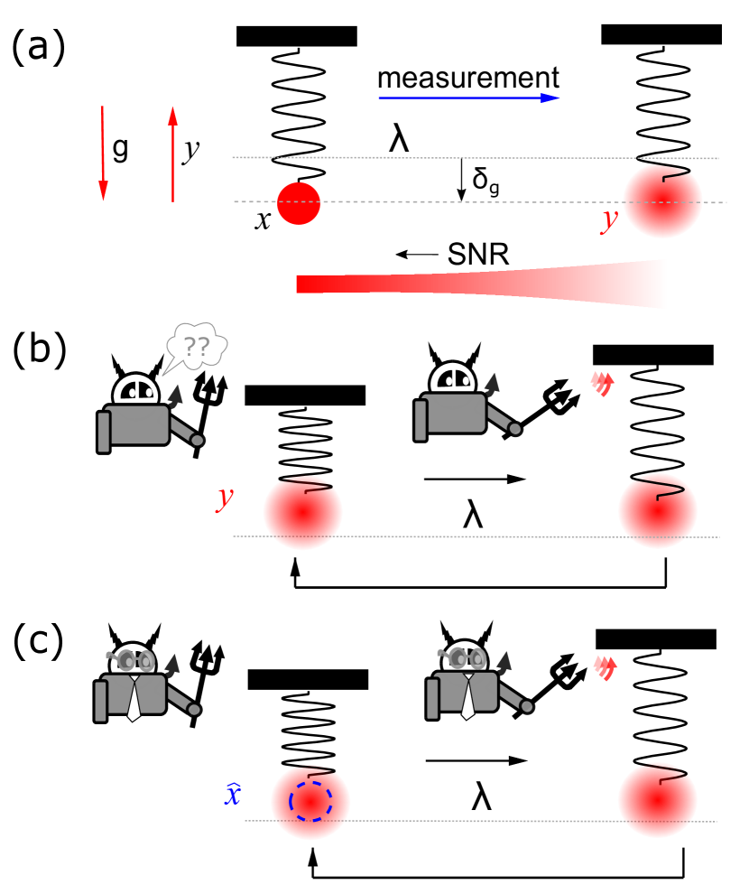
Experimental setup.—Our information engine consists of a 4-µm heavy bead trapped in a horizontally aligned optical trap. Because of the surrounding heat bath, the bead’s position fluctuates about an equilibrium average. The heavy bead is also subject to gravity. The bead’s position is measured with a sampling time µs using the scattered light from a detection laser.
In the operation of the engine, an observed “up” fluctuation increases the bead’s gravitational potential energy and can be captured (“rectified”) by a quick feedback response that shifts up the trap position. The response takes place after a one-time-step delay µs, with the shift chosen so that the trap does zero work on the bead. For this “pure” information engine, the work to run the motor is associated only with the measuring device and feedback controller, not the engine itself.
The optically trapped bead can be modeled by a spring-mass system [Fig. 1(a)]. The true position of the bead is estimated from a noisy measurement . Measurement noise is increased by reducing the intensity of the detection laser beam.
Figure 1(b) shows a naive information engine that directly uses a noisy measurement to apply feedback. By contrast, the Bayesian information engine bases its feedback on the best estimate of the bead’s position [Fig. 1(c)]. The bead’s position is estimated using a Bayesian filter that explicitly models the measurement noise and feedback delay 111The delay is also termed “feedback latency,” which refers explicitly to the sum of delays in the feedback loop, which include contributions from measurements, computations, and output to the actuator (the acousto-optic deflector, which moves the trap center). We use the more familiar informal language in the text..
The information engine can extract energy at high measurement noise because feedback decisions based on filtered estimates of the bead’s position are more likely to ratchet to a “true” upward fluctuation rather than to measurement noise.
Equations of motion.—The dynamics of the optically trapped bead obey an overdamped Langevin equation,
| (1) |
where is the position at time of a bead of diameter and effective (buoyant) mass in a trap of stiffness and center . The friction coefficient is , and is a Gaussian random variable with zero mean and covariance . We denote time derivatives by overdots. Scaling all lengths by the equilibrium position standard deviation and times by the bead relaxation time gives the nondimensionalized Langevin equation
| (2) |
for scaled effective mass .
Integrating Eq. (2) between measurements from to gives the discrete dynamics
| (3) |
for and . The variance of thermal force fluctuations depends on the sampling interval , and is a Gaussian random variable with zero mean and covariance .
The effect of measurement noise is modeled by a measurement variable that is the sum of the bead’s true position and additive white Gaussian noise,
| (4) |
with a Gaussian random variable with zero mean and covariance . We also assume that the thermal noise affecting the bead’s position is independent of the measurement noise: , for all and .
The trap position is updated at each time step using a “ratcheting rule,”
| (5) |
where denotes the Heaviside function, the feedback gain, and the estimate of the bead’s position (using either the naive measurement or the Bayesian estimate ). Because of delays, both the naive and Bayesian estimates of position use information from but not ; however, the Bayesian estimate also implicitly incorporates past information and uses the deterministic component of system dynamics to predict (see Eq. (6), below).
Estimating the bead position.—Since the actual bead position fluctuates on a scale and the measurement noise fluctuates on a scale , it is convenient to define a signal-to-noise ratio 222SNR is often alternately defined as a ratio of signal-to-noise power, .. In a first, naive approach to designing feedback based on noisy measurements, the feedback rule, Eq. (5), directly uses the measurement to update the trap position . Notice that this method implicitly estimates the position by . The naive method performs well at high SNR () but poorly at low SNR (), where a unidirectional ratchet (implemented via the Heaviside function) often responds to noise rather than actual bead movements.
In a second, filtering approach, we improve the estimate of by using a Fokker-Planck equation to predict the position probability given , which is itself calculated from measurements up to . One then updates (or “corrects”) the prediction for time by incorporating the measurement , using Bayes’ rule (see Appendix). For systems evolving according to linear dynamics and subject to Gaussian noise, remains Gaussian for all (if is initialized as Gaussian, see Appendix) and can be summarized by update equations for the mean and variance. The Bayesian filter is then known as the predictive Kalman filter, and one finds [compare Eq. (3)],
| (6) |
where the filter gain “corrects” the naive prediction using the difference between the previous estimate and actual observation (see Appendix and Ref. [25, Ch. 8]). The gain is chosen to minimize the variance between the true position and its estimate, and the resulting value is a function of the SNR. This variance is always less than that of the measurement noise ; it is optimal in that it incorporates all relevant past information contained in the (long) time series , and no other unbiased estimator—linear or not—has lower variance [26].
Engine thermodynamics.—Given an estimate of the bead’s position, we infer the thermodynamic quantities that characterize this engine’s performance. The rate at which we extract gravitational energy (i.e., change in bead free energy) during the time interval is [22]
| (7) |
and the time-averaged rate of free-energy change (more informally, the output power) is , where is the total duration of an -step protocol. We estimate the incremental input work (of the trap on the bead) as
| (8) |
which estimates input work based on the noisy measurement and not on the true position . The Appendix shows that this input-work estimator is unbiased—as a result of feedback delay.
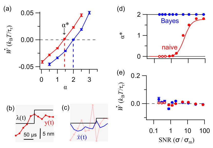
Results.—A “pure” information engine has zero input trap power: . For error-free measurements and no feedback delays, this criterion is satisfied at the critical feedback gain (see Appendix and Ref. [10]). Physically, this corresponds to translating the trap to a position opposite its minimum, so that the trap energy is unchanged. Feedback delay and measurement noise reduce . For our experimental conditions with delay of one time step and SNR = 10, is satisfied at the lower feedback gain [Fig. 2(a-b)].
The Bayesian information engine applies feedback based on the filtered predictive estimate of the bead’s position. As such, it accounts in its internal model for feedback delays and measurement noise.
Figure 2(a) shows the input trap power, at fixed SNR (=10), as a function of feedback gain . Despite the delay and finite SNR, the input trap power is zero for the “ideal” feedback gain . Figure 2(c) illustrates the operation of the Bayesian filter with a trajectory of the Bayesian information engine at lower SNR (). In contrast to the naive information engine, the trap ratchets only when the estimated position (blue) crosses the trap center (black), and not necessarily when the noisy measurement (light red) crosses the trap center.
Next, we investigate how depends on SNR, for the naive and Bayesian information engines. For the naive engine, decreases drastically at low SNR [Fig. 2(d)]. For , where denotes the critical vale of the SNR, a non-zero could not be found experimentally using the procedure outlined in Fig. 2(a). The Appendix shows that the vanishing of corresponds to a kind of phase transition between a regime where one can set while maintaining and a regime where one cannot.
By contrast, the critical feedback gain remains near 2 for the Bayesian engine [Fig. 2(d)]. The corresponding measured input trap powers for both the naive and Bayesian information engines are close to zero relative to the maximum output power () of the engine, at all SNR [Fig. 2(e)].
Taking advantage of predictions in our estimation algorithm thus simplifies the experiments, as it eliminates the need to empirically tune the feedback gain, ensuring that the zero-work condition is always satisfied at . Above, we saw that it also simplifies the work calculations needed to realize a pure information engine, as the value calculated directly from the noisy measurement is an unbiased estimator of the true work.
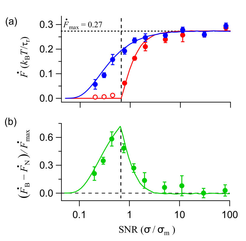
Finally, Fig. 3(a) compares the performance of the naive and Bayesian information engines, as quantified by the rate of stored gravitational power while keeping . Both output powers increase monotonically with SNR and saturate at the same power level at high SNR ().
Although the performance of Bayesian and naive information engines is similar at low and high SNR, there is a striking contrast at intermediate . Indeed, the difference of output powers (Bayesiannaive), normalized by , significantly exceeds zero for and reaches a maximum at (Fig. 3b).
At high SNR, the Bayesian filter “trusts the observation” and returns an estimate close to the instantaneous measurement, corrected for the expected bias due to the time delay. Since this bias is small for frequent measurements, both engines have similar performance and extract all the favorable thermal fluctuations, saturating at the maximum output power . At low SNR, the measurements are so noisy that they exceed the scale of the trap. The Bayesian information engine then extracts negligible power (see Appendix), while the naive engine extracts zero power. Therefore, at SNR and , the difference of output powers () tends to zero. But at intermediate SNR, the effective noise averaging in the Bayesian (Kalman) filter produces more accurate estimates, leading to better feedback decisions and thus improved engine performance.
To understand why the naive information engine shows a phase transition at a critical signal-to-noise ratio, we numerically solve a self-consistent equation for the SNR at which trap power vanishes. Enforcing the condition that is the unique solution (see Appendix), we find , consistent with both numerical simulations and experiments.
We also find that the phase transition arises from the biased estimate of the bead’s position from the noisy measurements. This bias has two origins: the delay due to feedback latency and the failure of the naive measurement to account for the fact that fluctuations above threshold are rare while noise fluctuations of either sign are equally likely. Because fluctuations up to the threshold are rare, the bead is usually below the observed value whenever an apparent threshold crossing is observed.
By contrast, a phase transition does not occur for the Bayesian information engine. The Bayesian filter gives an unbiased prediction of the bead’s position, accounting for both feedback delay and the “prior” associated with observations near the threshold. As a result, the bead is equally likely to be on either side of the predicted position, allowing one to tune for zero trap power and extract at least some power at any SNR value (see Appendix).
Conclusion.—Information engines that decide whether to ratchet using single noisy measurements have a phase transition at a critical signal-to-noise ratio and cannot function for . By contrast, if its feedback uses a Bayesian estimate of bead position that incorporates prior measurements, an information engine can operate at all values of SNR. The maximum performance benefit over the naive engine occurs at the critical value .
The ability to increase the performance of an information engine at low SNR is important for experimental investigations of motor mechanisms that use fluorescent probes [27]. In such applications, lower light intensities for monitoring fluorescent probes reduce photobleaching and allow longer measurements of motor behavior.
In addition, using a filtering algorithm to reduce the required accuracy of information while maintaining a given performance may decrease the thermodynamic costs of processing position measurements. Generally, a lower measurement accuracy reduces the minimum thermodynamic costs of running the controller [28, 14]. However, keeping a memory of past observations should increase those costs. Further work is needed to understand the efficiency of a feedback strategy that incorporates a memory of past measurements with one based purely on the most recent measurement. Such studies could evaluate the potential performance trade-offs encountered when varying the measurement accuracy.
Acknowledgements.
This research was supported by grant FQXi-IAF19-02 from the Foundational Questions Institute Fund, a donor-advised fund of the Silicon Valley Community Foundation. Additional support was from Natural Sciences and Engineering Research Council of Canada (NSERC) Discovery Grants (D.A.S. and J.B.) and a Tier-II Canada Research Chair (D.A.S.), an NSERC Undergraduate Summer Research Award, a BC Graduate Scholarship, and an NSERC Canadian Graduate Scholarship – Masters (J.N.E.L.).Appendix
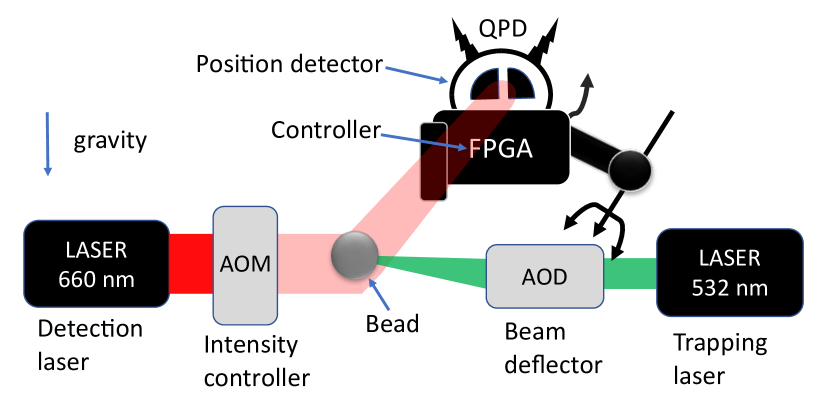
Appendix A Experimental apparatus
The experimental apparatus is designed to optically trap a bead in water. The optical trap is built by focusing a green laser using a water-immersion objective (Olympus, 60x 1.2 NA). The position of the trap is controlled using an acousto-optic deflector (AOD, AA opto-electronics). The position of the trapped bead is measured by a red detection laser, propagating anti-parallel to the trapping laser, that is loosely focused in the trapping plane using an air objective. The intensity of the detection bead is controlled using an acousto-optic modulator (AOM, AA opto-electronics) to vary the measurement noise. More details about the experimental apparatus can be found in [10, 29].
Appendix B Experimental parameter estimation
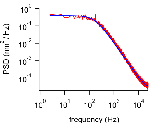
The trap stiffness, diffusion constant, and measurement noise are measured by fitting the power spectrum of the bead’s position to a discrete aliased Lorentzian [30]. The discrete equation of motion of the bead can be re-written as (cf. Eq. (3) in the main text)
| (S1) |
where is measured with respect to . The parameters are
| (S2) |
and
| (S3) |
where is the diffusion constant of the bead, the corner frequency, and the sampling time. Applying the discrete Fourier transform to the discrete equation of motion of the bead and calculating the expected value of the power spectrum , the discrete aliased Lorentzian is
| (S4) |
where indexes the discrete non-negative frequencies. For noisy measurements
| (S5) |
where the measurement noise is Gaussian white noise, the power spectrum of is
| (S6) |
where is the frequency-independent noise floor, and the variance of the measurement noise. Equation (S6) uses the property that the measurement noise is independent of both the bead’s position and thermal noise .
Appendix C Performance of Bayesian-filter estimator
When the measurement noise is additive Gaussian white noise and the system dynamics are linear, as is closely approximated in this experimental setup, an exactly solvable Bayesian filter can be designed to minimize the least-squares error between the filter’s state prediction and the true bead position. To derive the optimal filter for the information engine, we note that the bead’s motion is a first-order Markov process: its next position is conditionally independent of its history given its current position and the trap position , . Here, the probability is obtained from Eq. (3),
| (S7) | ||||
where denotes a normal distribution over with mean and variance . We also assume that the measurements of the bead’s position are memoryless: the measurement at the current time depends only on the current state, . Measurements with additive Gaussian white noise satisfy a distribution of the form
| (S8) |
The standard deviation of the noise distribution is the reciprocal of the signal-to-noise ratio, , and as such can be interpreted as a “noise-to-signal” ratio. Using Bayes’ rule, the update distribution is
| (S9) |
where is the set of measurements made up to and including time , and is a normalizing distribution. From this updated distribution and the dynamics (S7), the predicted distribution at the next discrete time is
| (S10) |
The measurement update and prediction steps for the information engine can be formulated as a sequence of transformations of univariate Gaussian probability densities. Since all densities are Gaussian, we need propagate only their means and variances:
| (S11a) | |||
| (S11b) | |||
Intuitively, the filter generates a prediction mean and variance (S11b), and . The stochastic bead dynamics increase the uncertainty of the bead’s position. This position uncertainty is reduced by the information obtained from the previous measurement . The reduction in prediction uncertainty and corresponding change to the prediction mean is achieved by feedback based on the discrepancy between the actual measurement and the prediction, . The Kalman gain multiplying this discrepancy accounts for the unreliability of the measurements, given the scale of measurement noise. The information engine uses this filter’s prediction mean as the estimate of the bead’s position in the feedback decision.
Appendix D Steady-state Bayesian-filter gain
In experiments, we assume that the experimental parameters do not change with time. As a result, the means and variances in the time-dependent Eqs. (S11) quickly approach steady-state values. To obtain the steady-state Bayesian-filter gain, we first solve the associated Riccati equation [25, Ch. 8] for the predictive variance,
| (S12) |
where superscript “SS” without time subscript indicates a steady-state quantity. The relevant solution to this quadratic equation is
| (S13) | ||||
We discard the other solution, as it is negative and variances must be positive. The resulting steady-state Bayesian (Kalman) filter gain is
| (S14) |
Finally, the Kalman-filtered position estimate is
| (S15) |
Appendix E Experimental implementation of the Bayesian filter
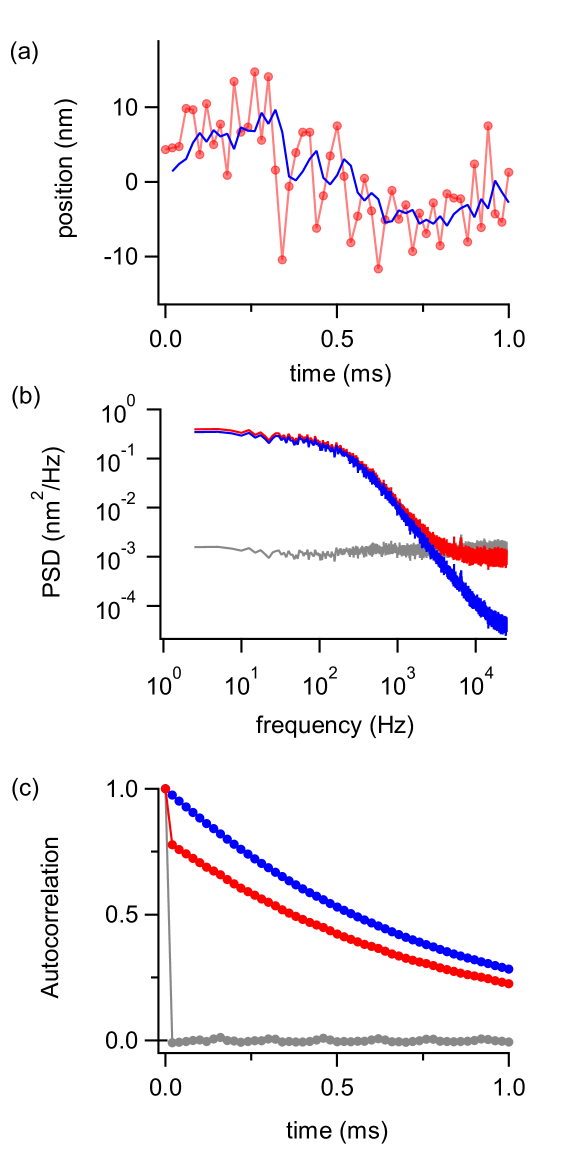
Experiments on the Bayesian information engine were performed using the Kalman-filtered position estimate obtained from Eq. (S15). Figure S3 shows the performance of the experimental implementation of the Kalman filter for a bead in a static trap. The experiment was performed at SNR 2, where the experimental parameters were estimated by fitting the power spectral density using Eq. (S6). Figure S3(a) shows the trajectory of the estimated bead position (blue), inferred using Eq. (S15) from the noisy measurements (red).
Figure S3(b) shows the power spectral densities of the noisy measurements (red) and Bayesian estimates (blue). The power spectral density of the noisy measurements saturates at a finite noise floor (PSD nm2/Hz). The filter-estimated position (blue) has a noise floor less then a tenth that of the individual noisy measurements (red). The power spectral density of the innovation is flat, showing that the innovations follow a white-noise distribution, and hence all the position correlations arising from the bead’s relaxation in the harmonic trap are extracted by the estimator.
Figure S3(c) shows the normalized autocorrelation of the noisy measurements (red), Bayesian estimates (blue), and innovations (gray). From Eq. (S5), the autocorrelation of the noisy measurements is
| (S16a) | ||||
| (S16b) | ||||
where we have again used the property that the measurement noise is independent of the true bead position.
The noisy measurements (red curve) show a delta-function peak at on top of a broader exponential decay, reflecting two processes: First, there is the contribution of measurement noise, which is delta correlated; second, there is the contribution of the dynamics, which has an exponential decay of correlations.
By contrast, the Bayesian estimate (blue curve) has only an exponential decay due to the dynamics—as would the autocorrelation function of noise-free dynamics. In other words, the Bayesian estimator distills the dynamical information in the correlated signal. The innovations (gray curve) are almost entirely delta correlated. Indeed, the degree to which the innovations approximate a delta function serves as a measure of the quality of the Bayesian filter. For example, deviations between a parameter value in the physical system and the corresponding model used for the Bayesian filter produce dynamical correlations in the innovations autocorrelation function [25]. Indeed, this mismatch has been used as a way to empirically tune parameters for Bayesian (Kalman) filters (“innovation whitening”) [31].
Appendix F Numerical-simulation methods
The numerical simulations generate multiple long trajectories of the bead using the discrete-time dynamics,
| (S17) |
where and . The corresponding noisy measurement is , where is a Gaussian random variable with zero mean and covariance . For the naive information engine, the trap position is updated using the feedback rule
| (S18) |
For the Bayesian information engine, the trap position is updated using the feedback rule
| (S19) |
using the Bayesian estimate (S15) of the bead’s position. For each engine type, the free-energy change is estimated using Eq. (7) and the work using the unbiased estimator Eq. (8) in the main text.
Appendix G Trap-work estimates are unbiased
Here, we show that our empirical estimator for the input trap work
| (S20) |
is an unbiased estimator when the feedback rule follows
| (S21) |
Note that this feedback rule updates the value of the control parameter at time according to the estimate of the bead’s position at the previous time , not the measurement that is made at the current time . In other words, there is a delay of one cycle between when a measurement is taken and when the corresponding feedback is applied.
For convenience, we introduce a new notation where the superscript on the thermodynamic quantities (e.g., ) denotes the type of measurement used in the estimation of the thermodynamic quantity. In this notation, we write (S20) as
| (S22) |
and the true estimate of the work from stochastic thermodynamics [32] given by the actual potential-energy change when updating to ,
| (S23) |
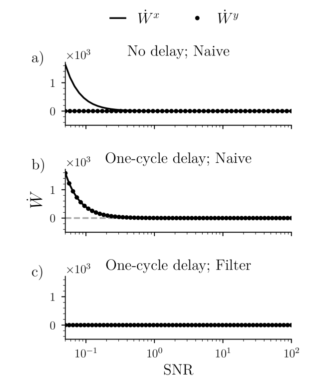
Now we compare the empirical estimates to the true values of the thermodynamic quantities. Expanding the definition of the empirical input work (S20) using , where is a zero-mean Gaussian random variable with variance , gives
| (S24a) | ||||
| (S24b) | ||||
| (S24c) | ||||
| (S24d) | ||||
Averaging over the noise at time , when the trap position has a nonnegative update (when , the work is trivially regardless of which position estimate is used), we find that
| (S25a) | ||||
| (S25b) | ||||
| (S25c) | ||||
| (S25d) | ||||
where, in the last step, we have used the property that both the position estimate (which denotes the noisy measurement in the naive case and the predictive estimate in the Bayesian case), and the trap position at time step are independent of the future measurement noise . Without the delay, the variables are correlated and the measurements are biased (Fig. S4a). This calculation suggests that feedback delay actually eliminates the bias in the empirical estimate of the trap work. Using numerical simulations, we compute the empirical power and find that it agrees well with the true values for both the naive (Fig. S4b) and Bayesian (Fig. S4c) information engines.
We also note that the trap work could alternatively be estimated using the Bayesian filtered position; however, the estimator in Eq. (S20) is robustly unbiased: It is unbiased even if the dynamical model used in the Kalman filter uses parameters that differ from those describing the physical system. The calculation of the trap position is based on past information and—whatever the algorithm used to compute its value—will always be independent of the current measurement.
Appendix H Experiment and simulation of the critical feedback gain
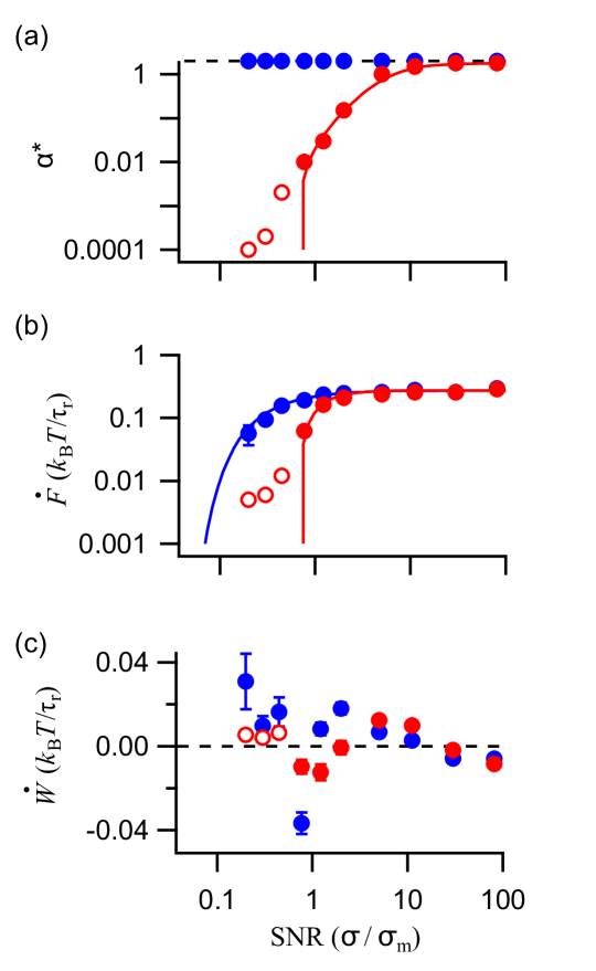
Figure S5 presents Fig. 2 in the main text, but with a logarithmic ordinate. According to simulations, for the naive information engine the critical feedback gain is the only solution below a critical signal-to-noise ratio , as shown in Fig. S5(a). At low SNR, experimental determinations of the critical feedback gain do not agree with numerical simulations (Fig. S5(a)), denoted as red hollow markers. Although experiments find , the naive output powers are still an order of magnitude smaller than those of the Bayesian information engine (Fig. S5(b)). Figure S5(c) shows the corresponding input trap powers , which remain small at low SNR.
Appendix I Theoretical arguments for the phase transition in the naive information engine
Empirically, the naive estimator can extract free energy only above a critical signal-to-noise ratio .
We define the critical SNR as the highest value for which is the only solution for which . Note that corresponds to never moving the trap and therefore not doing any work on the bead. When no feedback is performed, the stationary distribution of the bead inside the trap is the equilibrium Boltzmann distribution,
| (S26) |
This equation, the bead’s propagator in Eq. (S7), and the measurement distribution in Eq. (S8) together allow us to evaluate the input work,
| (S27a) | ||||
| (S27b) | ||||
| (S27c) | ||||
| (S27d) | ||||
| (S27e) | ||||
| (S27f) | ||||
where we substituted , , and in line (S27d), and used the normalization of the unknown in line (S27f).
Solving for yields solutions , and
| (S28) |
At the critical , the solution bifurcates. We determine the critical SNR from Eq. (S28) by solving
| (S29) |
for , which can only be done numerically. For and , the parameters used in Figs. 2 and 3,
| (S30) |
Figure 2 in the main text shows that this critical SNR indeed empirically coincides with the emergence of a positive . We note that the accuracy of this theoretical estimate (and thus the numerical precision we give) is limited by the accuracy of experimental parameters such as and which depend on the bead size.
Appendix J Experimental evidence supporting a phase transition in the naive information engine
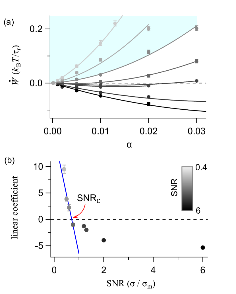
In this section, we present detailed experimental evidence for a phase transition in the naive information engine. Figure S6 (a) shows the trap power as a function of the feedback gain for different SNR, where the markers in the blue shaded region represent SNR values for which only positive trap powers () were measured. The experimental points are fit to a quadratic function; Fig. S6 (b) shows the linear coefficients of the fits in Fig. S6 (a) as a function of SNR. The measured slope switches from negative at high to positive at , consistent with determined in Eq. (S30). To measure the critical signal-to-noise ratio (where the linear coefficient is zero), the linear coefficients for SNRs 0.4–0.8 are linearly fit, giving an estimated zero linear coefficient and hence at . In the naive information engine experiments, for , we set because we cannot find an that leads to . Thus, the we report in such cases (red hollow markers in Fig. 3, main text) is an upper bound on the that satisfies : Either there is a smaller positive that we could not detect experimentally because differences in are too close to zero, or the only value that (always) enforces is . The corresponding measured using the upper-bound value of then is an upper bound on the output power for .
Appendix K The Bayesian information engine has no phase transition
Here, we present theoretical arguments to support the claim that there is no corresponding “phase transition” for the information engine that estimates the bead position using filtered measurements.
K.1 Feedback gain
First, we show that feedback gain generally produces vanishing input work. Using the predictive Kalman filter [Eq. (6)] in the feedback rule [Eq. (5)] with , the trap work is
| (S31a) | ||||
| (S31b) | ||||
| (S31c) | ||||
| (S31d) | ||||
| (S31e) | ||||
where (S31d) used the fact that the posterior distribution of the true bead position is symmetric around the filter estimate , which in this case is the mean of the Gaussian posterior. Figure S7 shows the input work as a function of the feedback gain for different signal-to-noise ratios. makes the input work vanish.
K.2 Free-energy gain
With feedback gain and the feedback rule in Eq. (5), the free energy-gain per time step, Eq. (7), becomes
| (S32a) | |||
| (S32b) | |||
| (S32c) | |||
where we used the fact that the probability density is positive and always has a tail (however small) reaching into the region . Hence, there is no phase transition in the Bayesian information engine. Note that for the naive engine
| (S33) |
which vanishes for .
To corroborate the finding that the Bayesian information engine has no phase transition, we calculate the low-SNR limit of the free-energy gain per time step. When SNR is low, feedback is applied rarely and hence the stationary distribution of bead positions approximates the equilibrium Boltzmann distribution, . Hence, the distribution of filter estimates is also approximately Gaussian,
| (S34) |
The mean and variance (S11b) of the predictive Kalman filter dictate the steady-state the posterior distribution, of the true bead position given the filter estimate ,
| (S35) |
allowing us to solve for ,
| (S36) |
such that
| (S37a) | ||||
| (S37b) | ||||
are the mean and variance of the filter state in Eq. (S36).
Inserting these cumulants into Eq. (S34) and evaluating Eq. (S32b) again using the normalization of gives
| (S38) |
Expanding the stationary filter variance (S13) for small yields
| (S39) |
Then, with for ,
| (S40) |
illustrating that the Bayesian information ratchet extracts free energy at all signal-to-noise ratios.
References
- Parrondo et al. [2015] J. M. Parrondo, J. M. Horowitz, and T. Sagawa, Thermodynamics of information, Nat. Phys. 11, 131 (2015).
- Toyabe et al. [2010] S. Toyabe, T. Sagawa, M. Ueda, E. Muneyuki, and M. Sano, Experimental demonstration of information-to-energy conversion and validation of the generalized Jarzynski equality, Nat. Phys. 6, 988 (2010).
- Camati et al. [2016] P. A. Camati, J. P. Peterson, T. B. Batalhão, K. Micadei, A. M. Souza, R. S. Sarthour, I. S. Oliveira, and R. M. Serra, Experimental rectification of entropy production by Maxwell’s demon in a quantum system, Phys. Rev. Lett. 117, 240502 (2016).
- Koski et al. [2015] J. V. Koski, A. Kutvonen, I. M. Khaymovich, T. Ala-Nissila, and J. P. Pekola, On-chip Maxwell’s demon as an information-powered refrigerator, Phys. Rev. Lett. 115, 260602 (2015).
- Chida et al. [2017] K. Chida, S. Desai, K. Nishiguchi, and A. Fujiwara, Power generator driven by Maxwell’s demon, Nat. Commun. 8, 1 (2017).
- Kumar et al. [2018] A. Kumar, T.-Y. Wu, F. Giraldo, and D. S. Weiss, Sorting ultracold atoms in a three-dimensional optical lattice in a realization of Maxwell’s demon, Nature 561, 83 (2018).
- Thorn et al. [2008] J. J. Thorn, E. A. Schoene, T. Li, and D. A. Steck, Experimental realization of an optical one-way barrier for neutral atoms, Phys. Rev. Lett. 100, 240407 (2008).
- Vidrighin et al. [2016] M. D. Vidrighin, O. Dahlsten, M. Barbieri, M. Kim, V. Vedral, and I. A. Walmsley, Photonic Maxwell’s demon, Phys. Rev. Lett. 116, 050401 (2016).
- Saha and Bechhoefer [2021] T. K. Saha and J. Bechhoefer, Trajectory control using an information engine, in Optical Trapping and Optical Micromanipulation XVIII, Vol. 11798 (International Society for Optics and Photonics, 2021) p. 117980L.
- Saha et al. [2021] T. K. Saha, J. N. E. Lucero, J. Ehrich, D. A. Sivak, and J. Bechhoefer, Maximizing power and velocity of an information engine, Proc. Natl. Acad. Sci. U.S.A. 118 (2021).
- Paneru et al. [2018] G. Paneru, D. Y. Lee, T. Tlusty, and H. K. Pak, Lossless Brownian information engine, Phys. Rev. Lett. 120, 020601 (2018).
- Admon et al. [2018] T. Admon, S. Rahav, and Y. Roichman, Experimental realization of an information machine with tunable temporal correlations, Phys. Rev. Lett. 121, 180601 (2018).
- Ribezzi-Crivellari and Ritort [2019] M. Ribezzi-Crivellari and F. Ritort, Large work extraction and the Landauer limit in a continuous Maxwell demon, Nat. Phys. 15, 660 (2019).
- Paneru et al. [2020] G. Paneru, S. Dutta, T. Sagawa, T. Tlusty, and H. K. Pak, Efficiency fluctuations and noise induced refrigerator-to-heater transition in information engines, Nat. Commun. 11, 1 (2020).
- Taghvaei et al. [2022] A. Taghvaei, O. M. Miangolarra, R. Fu, Y. Chen, and T. T. Georgiou, On the relation between information and power in stochastic thermodynamic engines, IEEE Control Syst. Lett. 6, 434 (2022).
- Nakamura and Kobayashi [2021] K. Nakamura and T. J. Kobayashi, Connection between the bacterial chemotactic network and optimal filtering, Phys. Rev. Lett. 126, 128102 (2021).
- Horowitz et al. [2013] J. M. Horowitz, T. Sagawa, and J. M. Parrondo, Imitating chemical motors with optimal information motors, Phys. Rev. Lett. 111, 010602 (2013).
- Rupprecht and Vural [2020] N. Rupprecht and D. C. Vural, Predictive Maxwell’s demons, Phys. Rev. E 102, 062145 (2020).
- Fields and Cohen [2011] A. P. Fields and A. E. Cohen, Electrokinetic trapping at the one nanometer limit, Proc. Natl. Acad. Sci. U.S.A. 108, 8937 (2011).
- Magrini et al. [2021] L. Magrini, P. Rosenzweig, C. Bach, A. Deutschmann-Olek, S. G. Hofer, S. Hong, N. Kiesel, A. Kugi, and M. Aspelmeyer, Real-time optimal quantum control of mechanical motion at room temperature, Nature 595, 373 (2021).
- Conangla et al. [2019] G. P. Conangla, F. Ricci, M. T. Cuairan, A. W. Schell, N. Meyer, and R. Quidant, Optimal feedback cooling of a charged levitated nanoparticle with adaptive control, Phys. Rev. Lett. 122, 223602 (2019).
- Lucero et al. [2021] J. N. E. Lucero, J. Ehrich, J. Bechhoefer, and D. A. Sivak, Maximal fluctuation exploitation in Gaussian information engines, Phys. Rev. E 104, 044122 (2021).
- Note [1] The delay is also termed “feedback latency,” which refers explicitly to the sum of delays in the feedback loop, which include contributions from measurements, computations, and output to the actuator (the acousto-optic deflector, which moves the trap center). We use the more familiar informal language in the text.
- Note [2] SNR is often alternately defined as a ratio of signal-to-noise power, .
- Bechhoefer [2021] J. Bechhoefer, Control Theory for Physicists (Cambridge University Press, 2021).
- Kailath et al. [2000] T. Kailath, A. H. Sayed, and B. Hassibi, Linear Estimation (Prentice Hall, 2000).
- Veigel and Schmidt [2011] C. Veigel and C. F. Schmidt, Moving into the cell: single-molecule studies of molecular motors in complex environments, Nat. Rev. Mol. Cell Biol. 12, 163 (2011).
- Horowitz and Sandberg [2014] J. M. Horowitz and H. Sandberg, Second-law-like inequalities with information and their interpretations, New J. Phys. 16, 125007 (2014).
- Kumar and Bechhoefer [2018] A. Kumar and J. Bechhoefer, Nanoscale virtual potentials using optical tweezers, Appl. Phys. Lett. 113, 183702 (2018).
- Berg-Sørensen and Flyvbjerg [2004] K. Berg-Sørensen and H. Flyvbjerg, Power spectrum analysis for optical tweezers, Rev. Sci. Instrum. 75, 594 (2004).
- Wang and Moerner [2011] Q. Wang and W. E. Moerner, An adaptive anti-Brownian electrokinetic trap with real-time information on single-molecule diffusivity and mobility, ACS Nano 7, 5792 (2011).
- Sekimoto [2010] K. Sekimoto, Stochastic Energetics (Springer, 2010).