A Geometric Approach on Circular Photon Orbits and Black Hole Shadow

Abstract

Circular photon orbit and black hole shadow are significantly important issues in physics and astronomy, and a number of breakthroughs have been witnessed in recent years. Conventionally, the stable and unstable circular photon orbits are obtained using the effective potential of test particles moving in black hole spacetime. In this work, a pure geometric approach is developed to calculate these circular photon orbits and black hole shadow radius. Furthermore, it can be proved that our geometric approach is completely equivalent to the conventional approach based on effective potentials of test particles.

Backgrounds and Introduction: Black holes are massive compact objects predicted by Einstein’s general theory of relativity. They have attracted large numbers of interests in high-energy physics, astrophysics and astronomy over the past decades. Significantly important information on gravitation, galaxies, thermodynamics and quantum effects in curved spacetime can be revealed from black holes [1, 2, 3, 4, 5]. Recently, huge progresses in black hole physics have been witnessed. The gravitational wave signals from binary black hole mergers were detected by LIGO and Virgo [6, 7]. The high resolution images of supermassive black hole at the center of galaxy M87 were captured by Event Horizon Telescope (EHT) [8, 9].

The circular photon orbit and shadow radius are important features for black holes. The particle motions, gravitational lensing, optical imaging and other aspects of black hole can be studied from these quantities. Since the observation of black hole image in galaxy M87 by EHT collaboration, the circular photon orbits and black hole shadow have became extremely hot topics in physics and astronomy. Conventionally, these circular photon orbits and black hole shadow radius can be calculated from the effective potential of test particles moving in black hole spacetime [10, 11, 12, 13, 14, 15, 17, 18, 16]. In recent years, other approaches on circular photon orbits (photon sphere, light rings) using topological and geometric techniques also emerged [19, 20, 21, 22].

In the present work, a pure geometric approach is developed to obtain the stable and unstable circular photon orbits, as well as black hole shadows. Our approach is implemented in the optical geometry of black hole spacetime. In this approach, the geodesic curvature and Gauss curvature in optical geometry turn out to be crucial quantities to determine the circular photon orbits. The stability of circular photon orbits is reflected by an elegant theorem in differential geometry and topology —— the Hadamard theorem. Furthermore, in this work, we also prove that the geometric approach developed in this work is completely equivalent to the conventional approach based on effective potential of test particles.

Optical Geometry of Black Hole Spacetime: The optical geometry is a powerful tool to study the motions of photons (or other massless particles which travel along null geodesics) in gravitational field. [23, 24, 25, 26]. For a four dimensional spacetime, its optical geometry can be constructed from the null constraint $d\tau^{2}=0$.

$$\underbrace{d\tau^{2}=g_{\mu\nu}dx^{\mu}dx^{\nu}}_{\text{Spacetime Geometry}}\ \ \overset{d\tau^{2}=0}{\Longrightarrow}\ \ \underbrace{dt^{2}=g^{\text{OP}}_{ij}dx^{i}dx^{j}}_{\text{Optical Geometry}}$$ (1)

The properties of optical geometry are strongly depend on the symmetries of gravitational field and black hole spacetime. For a spherically symmetric black hole, its optical geometry gives a Riemannian manifold [23, 24, 25]. However, for a rotational black hole, the correspond optical geometry is a Randers-Finsler manifold [26, 27, 29, 28]. Further, if we consider particle motions in the equatorial plane, a two dimensional manifold can be constructed from the optical geometry.

$$\underbrace{dt^{2}=g^{\text{OP}}_{ij}dx^{i}dx^{j}}_{\text{Optical Geometry}}\ \ \overset{\theta=\pi/2}{\Longrightarrow}\ \ \underbrace{dt^{2}=\tilde{g}^{\text{OP}}_{ij}dx^{i}dx^{j}}_{\text{Optical Geometry (Two Dimensional)}}$$ (2)

In two dimensional manifold, a number of elegant and classical theorems in surface theory and differential geometry could provide useful tools to study the particle motions. In this work, our new geometric approach on circular photon orbits and black hole shadow is implemented in two dimensional optical geometry. A detailed description of optical geometry is given in supplemental material.

Gauss Curvature and Geodesic Curvature: There are several key quantities which describe the geometric properties of optical geometry. It would be turned out that Gauss curvature and geodesic curvature in optical geometry play central roles in determining the circular photon orbits for black holes. The Gauss curvature is the intrinsic curvature of a two dimensional surface. The geodesic curvature is the curvature of one dimensional curves lived in two dimensional curved surface, which measures how far these curves are from being geodesics. If $\gamma$ is a geodesic curve in surface $S$, its geodesic curvature $\kappa_{g}(\gamma)$ automatically vanishes. Notably, both Gauss curvature and geodesic curvature only rely on the intrinsic metric of two dimensional surface $S$, regardless of the embedding of this surface into higher dimensional spacetime [30]. More discussions on Gauss curvature and geodesic curvature can be found in the supplemental material.

Circular Photon Orbit: The circular photon orbits are important features of black holes. They are closely connected with particle motions, gravitational lensing and black hole shadows. The circular photon orbits are classified into two categories: the stable and unstable circular photon orbits. They may exhibit significantly different features, especially for the geodesics nearby. For unstable circular photon orbit, when photon beams have a departure from the circular orbit, they would either fall into black hole or move to infinity. No bound photon orbits are admitted near the unstable circular photon orbit. Conversely, there are many bound photon orbits near the stable circular photon orbit. These bound photon orbits may have different shapes. The stable and unstable circular photon orbits are illustrated in figure 1.

In this work, a pure geometric approach is developed to obtain these circular photon orbits. We choose a class of stationary and spherically symmetric black holes to show our geometric approach. For spherically symmetric black hole with the metric

$$d\tau^{2}=f(r)dt^{2}-\frac{1}{f(r)}dr^{2}-r^{2}(d\theta^{2}+r^{2}\sin^{2}\theta d\phi^{2})$$ (3)

the optical geometry restricted in the equatorial plane $\theta=\pi/2$ gives

$$dt^{2}=\tilde{g}^{\text{OP}}_{ij}dx^{i}dx^{j}=\frac{1}{[f(r)]^{2}}dr^{2}+\frac{r^{2}}{f(r)}d\phi^{2}$$ (4)

Here, we only restrict to a subclass of static and spherically symmetric black hole such that the spacetime metric satisfies $g_{tt}\times g_{rr}=-1$ and $g_{\theta\theta}=r^{2}$. The cases of more general spherically symmetric and rotational (axisymmetric) black holes are left to incoming studies.

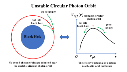
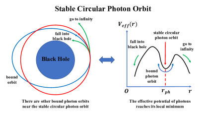
Figure 1: The schematic plot of the stable and unstable circular photon orbits near black holes. In this figure, we choose the spherically symmetric black hole as a typical example, and the region covered by blue is the interior of black hole.

The circular photon orbits could be determined by Gauss curvature and geodesic curvature in optical geometry. Firstly, for circular photon orbit $r=r_{ph}$, which is a geodesic curve in optical geometry, its geodesic curvature vanishes naturally [32, 33, 40]

$$\kappa_{g}(r=r_{ph}) = \frac{1}{2\sqrt{\tilde{g}^{\text{OP}}_{rr}}}\frac{\partial\ log(\tilde{g}^{\text{OP}}_{\phi\phi})}{\partial r}\bigg{|}_{r=r_{ph}}$$ (5)

$$= \bigg{[}\frac{f(r)}{r}-\frac{1}{2}\cdot\frac{\partial f(r)}{\partial r}\bigg{]}_{r=r_{ph}}=0$$

In this way, the radius of circular photon orbit is obtained. Here, we should emphasize that an important property of optical geometry is used in deriving this relation. The null geodesic curve $\gamma=\gamma(\tau)$ in the spacetime geometry $d\tau^{2}=g_{\mu\nu}dx^{\mu}dx^{\nu}$ maintains geodesic in the optical geometry $dt^{2}=g^{\text{OP}}_{ij}dx^{i}dx^{j}$ [25]. Actually, it can be viewed as the generalization of Fermat’s principle in curved stationary spacetime [25, 26, 38].

The following question is how to distinguish stable photon orbits from unstable photon orbits. The following Hadamard theorem in differential geometry would answer this question appropriately.

Hadamard Theorem: For a two dimensional complete Riemannian manifold with nonpositive Gauss curvature, there is only one geodesic curve from $p$ to $q$ belong to the same homotopy class, and this geodesic curve minimizes the length in this homotopy class [34, 35].

For spherically symmetric black hole, if we restrict the optical geometry in two dimensional equatorial plane, the Gauss curvature in the Hadamard theorem can be calculated through [32, 33]

$$\mathcal{K} = -\frac{1}{\sqrt{\tilde{g}^{\text{OP}}}}\bigg{[}\frac{\partial}{\partial\phi}\bigg{(}\frac{1}{\sqrt{\tilde{g}^{\text{OP}}_{\phi\phi}}}\frac{\partial\sqrt{\tilde{g}^{\text{OP}}_{rr}}}{\partial\phi}\bigg{)}+\frac{\partial}{\partial r}\bigg{(}\frac{1}{\sqrt{\tilde{g}^{\text{OP}}_{rr}}}\frac{\partial\sqrt{\tilde{g}^{\text{OP}}_{\phi\phi}}}{\partial r}\bigg{)}\bigg{]}$$ (6)

$$= \frac{1}{2}f(r)\cdot\frac{d^{2}f(r)}{dr^{2}}-\bigg{[}\frac{1}{2}\cdot\frac{df(r)}{dr}\bigg{]}^{2}$$

where $\tilde{g}^{\text{OP}}=det(\tilde{g}^{\text{OP}}_{ij})$ is determinant of optical metric.

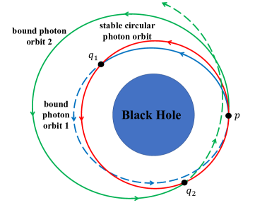
Figure 2: This figure shows several possible bound photon orbits near the stable circular photon orbits. These bound photon orbits could be obtained by perturbation of circular photon orbit at point $p$, and they may have different shapes. The bound photon orbit $1$ labeled in blue is a closed orbit, and the bound photon orbit $2$ labeled in green is an unclosed orbit (just like the Mercury procession around the Sun). In the equatorial plane of optical geometry, we can find another point $q$ (we denote the $q_{i}$ for bound orbit $i=1,2$). When we considering photon orbits starting from $p$ ending with $q$, there are at least two different photon orbits (one is the stable circular photon orbit, and the other is a bound photon orbit) that can be continuously deformed to each other. Therefore, in the equatorial plane of optical geometry, there are two different geodesic curves from $p$ to $q$ belong to the same homotopy class.

For stable circular photon orbit, there are bound photon orbits nearby, which may have different shapes. In the equatorial plane of optical geometry, we can find two points $p$ and $q$ such that there are at least two geodesic curves (one is the stable photon orbit, the other is a bound photon orbit) belong to the same homotopy class. Figure 2 illustrates two possible bound photon orbits and the corresponding choice of points $p$ and $q$. In such cases, the Gauss curvature of optical geometry should be positive, otherwise it would violate the Hadamard theorem. On the contrary, for unstable circular photon orbit, no bound photon orbits homotopic to this circular photon orbit exist. Then unstable circular photon orbit itself forms the whole homotopy class, which correspond to the negative Gauss curvature in the Hadamard theorem (we assume the Gauss curvature of optical geometry is nonzero, otherwise the black hole spacetime would by flat). Based on the above discussions, we obtain the following criterion to determine the stable and unstable circular photon orbits [39].

$$\mathcal{K}<0 \Rightarrow r=r_{ph}$$ The circular photon orbit is unstable

$$\mathcal{K}>0 \Rightarrow r=r_{ph}$$ The circular photon orbit is stable

Black Hole Shadow: Black hole shadow is the dark silhouette of black hole image in a bright background. The size and shape of black hole shadow depends not only on black hole parameters, but also on the position of observers [17]. In this work, we concentrate on the idealized situation where observer is located at infinity, and there are no light sources between the observer and black hole. In this case, the radius of black hole shadow detected by observer is just the critical value of impact parameter $b_{\text{critical}}$. In the gravitational field, light beams emitted from infinity with impact parameter $b=b_{\text{critical}}$ would reach the unstable circular photon orbit exactly, as illustrated in figure 3

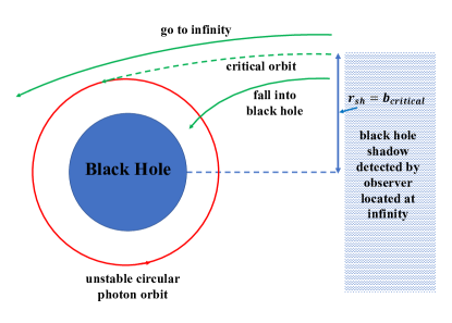
Figure 3: The black hole shadow and unstable circular photon orbit. The light beam emitted from infinity with impact parameter $b=b_{\text{critical}}$ would reach the unstable circular photon orbit exactly. The light beam emitted with impact parameter $b<b_{\text{critical}}$ would fall into the black hole.

Table 1: The circular photon orbit and black hole shadow radius detected by observer at infinity. This table summarize the results for Schwarzschild black hole and Reissner-Nordström black hole. All quantities calculated using our new geometric approach agree with the results obtained using conventional approach based on effective potential.

	Type of Black Hole	Schwarzschild Black Hole	Reissner-Nordström Black Hole
	Metric	$f(r)=1-2M/r$	$f(r)=1-2M/r+Q^{2}/r^{2}$
	Geodesic Curvature	$\kappa_{g}=1/r-3M/r^{2}$	$\kappa_{g}=1/r-3M/r^{2}+2Q^{2}/r^{3}$
	Circular Photon Orbit	$r_{ph}=3M$	$r_{ph}=(3M+\sqrt{9M^{2}-8Q^{2}})/2$
	Gauss Curvature	$\mathcal{K}=-2M/r^{3}+3M^{2}/r^{4}<0$	$\mathcal{K}=-2M/r^{3}+3(M^{2}+Q^{2})/r^{4}-6MQ^{2}/r^{5}+2Q^{4}/r^{6}<0$
		(outside black hole horizon, $r>2M$)	(outside black hole horizon, $r>M+\sqrt{M^{2}-Q^{2}}$)
	Stability	$r_{ph}=3M$ is unstable circular orbit.	$r_{ph}=(3M+\sqrt{9M^{2}-8Q^{2}})/2$ is unstable circular orbit.
	Black Hole Shadow	$r_{sh}=b_{\text{critical}}=3\sqrt{3}M$	$r_{sh}=b_{\text{critical}}=\frac{(3M+\sqrt{9M^{2}-8Q^{2}})^{2}}{\sqrt{8(3M^{2}-2Q^{2}+M\sqrt{9M^{2}-8Q^{2}})}}$

Following the conventional definition, the impact parameter can be expressed as [15]

$$b\equiv\bigg{|}\frac{L}{E}\bigg{|}=\bigg{|}\frac{r^{2}\sin^{2}\theta\cdot d\phi/d\lambda}{f(r)\cdot dt/d\lambda}\bigg{|}$$ (7)

where $E$ and $L$ is the conserved energy and angular momentum per unit mass

$$E=f(r)\cdot\frac{dt}{d\lambda}$$ (8a)

$$L=r^{2}\sin^{2}\theta\cdot\frac{d\phi}{d\lambda}$$ (8b)

Since the impact parameter $b\equiv L/E$ is a conserved quantity along the geodesics, we can calculate the critical impact parameter $b_{\text{critical}}$ at any specific point along the photon trajectory. A simple and convenient choice are the points in the unstable circular photon orbit $r=r_{\text{unstable}}$

$$b_{\text{critical}}=\bigg{|}\frac{L}{E}\bigg{|}_{r=r_{\text{unstable}}}=\bigg{|}\frac{r^{2}}{f(r)}\cdot\frac{d\phi/d\lambda}{dt/d\lambda}\bigg{|}_{r=r_{\text{unstable}}}$$ (9)

where $\theta=\pi/2$ has been used in the equatorial plane.

The radius of black hole shadow detected by observer at infinity can be calculated in the optical geometry. In the spacetime geometry, photon orbits are along lightlike / null geodesics, and their tangent vector satisfies $T\cdot T=g_{\mu\nu}\frac{dx^{\mu}}{d\lambda}\frac{dx^{\nu}}{d\lambda}=0$, with $\lambda$ to be any affine parameter of null geodesics. However, when transformed into the optical geometry, the photon orbits become spatial geodesics with vanishing geodesic curvature $\kappa_{g}=0$, as we have emphasized previously [40]. The stationary time coordinate $t$ in spacetime geometry exactly reduces to the arc-length parameter / spatial distance parameter in optical geometry. In the optical geometry, the tangent vector of arbitrary photon orbits $T^{\text{OP}}=d/dt$ with respect to arc-length parameter $t$ becomes a unit vector ($|T^{\text{OP}}|=1$). Here, we restrict the optical geometry in the equatorial plane, the tangent vector of photon orbits reduce to $T^{\text{OP}}=(\frac{dr}{dt},\frac{d\phi}{dt})$. Furthermore, for unstable circular photon orbit, we have the result

$$r=r_{\text{unstable}}=\text{constant}\ \Rightarrow\ \frac{dr}{dt}\bigg{|}_{r=r_{\text{unstable}}}=0$$

$$\Rightarrow |T^{\text{OP}}\cdot T^{\text{OP}}|=\bigg{|}\tilde{g}^{\text{OP}}_{\phi\phi}\cdot\frac{d\phi}{dt}\cdot\frac{d\phi}{dt}\bigg{|}$$

$$\ \ \ \ \ \ \ \ \ \ \ \ \ \ \ \ =\bigg{|}\frac{r^{2}}{f(r)}\cdot\frac{d\phi}{dt}\cdot\frac{d\phi}{dt}\bigg{|}_{r=r_{\text{unstable}}}=1$$

$$\Rightarrow r_{sh}=b_{\text{critical}}=\bigg{|}\frac{r^{2}}{f(r)}\cdot\frac{d\phi/d\lambda}{dt/d\lambda}\bigg{|}_{r=r_{\text{unstable}}}=\sqrt{\frac{r_{\text{unstable}}^{2}}{f(r_{\text{unstable}})}}$$

This is the analytical expression for black hole shadow radius detected by observer located at infinity, and it is consistent with previous results [13, 17]. Based on above procedures, the shadow radius for arbitrary spherically symmetric black hole with metric from in equation (3) can be calculated. In the present work, we choose two typical examples in general relativity —— Schwarzschild black hole and Reissner-Nordström black hole. The circular photon orbits and black hole shadow radius for these black holes are summarized in table 2.

Equivalence between Our Geometric Approach and Conventional Approach: The geometric approach developed in this work is completely equivalent to the conventional approach based on effective potentials of test particles moving in the gravitational field. In conventional approach, the circular photon orbit can be solved by analyzing the extreme points of effective potential $V_{\text{eff}}(r)$. Particularly, the unstable circular photon orbit $r=r_{\text{unstable}}$ corresponds to local maximum of effective potential, and the stable circular photon orbit $r=r_{\text{stable}}$ is the local minimum of effective potential.

Table 2: The features of our geometric approach developed in this work and the conventional approach.

	Approach	Our Geometric Approach	Conventional Approach
	Geometry	Optical Geometry of Spacetime	Spacetime Geometry
		(Riemannian / Randers-Finsler Geometry)	(Lorentz Geometry)
	Key Quantities	Gauss Curvature $\mathcal{K}(r)$	Effective Potential $V_{\text{eff}}(r)$
		Geodesic Curvature $\kappa_{g}(r)$
	Photon Orbit	Conditions	Conditions
	circular photon orbit	zero geodesic curvature	extreme point of effective potential
		$\kappa_{g}(r)=0$	$\frac{dV_{\text{eff}}(r)}{dr}=0$
	unstable circular photon orbit	zero geodesic curvature and negative Gauss curvature	local maximum of effective potential
		$\kappa_{g}(r)=0$ and $\mathcal{K}(r)<0$	$\frac{dV_{\text{eff}}(r)}{dr}=0$ and $\frac{d^{2}V_{\text{eff}}(r)}{dr^{2}}<0$
	stable circular photon orbit	zero geodesic curvature and positive Gauss curvature	local minimum of effective potential
		$\kappa_{g}(r)=0$ and $\mathcal{K}(r)>0$	$\frac{dV_{\text{eff}}(r)}{dr}=0$ and $\frac{d^{2}V_{\text{eff}}(r)}{dr^{2}}>0$

We now demonstrate the equivalence between these two approaches. In spherically symmetric black hole spacetime, if we restrict test particles moving in the equatorial plane $\theta=\pi/2$, the equation of motion eventually reduces to [14]

$$\frac{1}{2}\cdot\bigg{(}\frac{dr}{d\lambda}\bigg{)}^{2}+V_{\text{eff}}(r)=\frac{1}{2}\cdot E^{2}$$ (11)

where effective potential of test particles is defined by

$$V_{\text{eff}}(r)\equiv\frac{f(r)}{2}\cdot\bigg{(}\frac{L^{2}}{r^{2}}+\epsilon\bigg{)}$$ (12)

Here, for massless particles $\epsilon=0$, and for massive particles $\epsilon=1$. The circular photon orbit $r=r_{ph}$ correspond to the extreme point of effective potential [14, 15]

$$\frac{dV_{\text{eff}}(r)}{dr}\bigg{|}_{r=r_{ph}}=0$$ (13)

$$\Rightarrow \bigg{[}\frac{L^{2}}{2r^{2}}\cdot\frac{df(r)}{dr}-\frac{L^{2}\cdot f(r)}{r^{3}}\bigg{]}_{r=r_{ph}}=0$$

where we have used $\epsilon=0$ for massless photons. Note that the angular momentum $L$ is a conserved quantity along photon orbit, which is independent of $r$. Comparing equation (13) with equation (5), it is clearly demonstrated that they are equivalent to each other. When $r=r_{ph}$ is the extreme point of effective potential $V_{\text{eff}}(r)$, the geodesic curvature along the circle $r=r_{ph}$ vanishes precisely, which makes it to be the circular photon orbit for spherically symmetric black holes.

Then we analyze the stability of circular photon orbits. For unstable circular photon orbit $r=r_{\text{unstable}}$, the effective potential should reach its local maximum [15, 18]

$$\frac{d^{2}V_{\text{eff}}(r)}{dr^{2}}\bigg{|}_{r=r_{\text{unstable}}}<0$$ (14)

$$\Rightarrow \bigg{[}\frac{L^{2}}{2r^{2}}\cdot\frac{d^{2}f(r)}{dr^{2}}-\frac{2L^{2}}{r^{3}}\cdot\frac{df(r)}{dr}+\frac{3L^{2}\cdot f(r)}{r^{4}}\bigg{]}_{r=r_{\text{unstable}}}<0$$

$$\Rightarrow \bigg{[}\frac{L^{2}}{2r^{2}}\cdot\frac{d^{2}f(r)}{dr^{2}}-\frac{L^{2}\cdot f(r)}{r^{4}}\bigg{]}_{r=r_{\text{unstable}}}<0$$

$$\Rightarrow \bigg{[}\frac{f(r)}{2}\cdot\frac{d^{2}f(r)}{dr^{2}}-\frac{f(r)\cdot f(r)}{r^{2}}\bigg{]}_{r=r_{\text{unstable}}}<0$$

$$\Rightarrow \bigg{[}\frac{f(r)}{2}\cdot\frac{d^{2}f(r)}{dr^{2}}-\bigg{(}\frac{1}{2}\frac{df(r)}{dr}\bigg{)}^{2}\bigg{]}_{r=r_{\text{unstable}}}<0$$

In the derivation, we have used the relation $df(r)/dr=2f(r)/r$ in equation (13) for unstable circular photon orbit repeatedly. Recall the expression for Gauss curvature in equation (6), the last line of this inequality implies that Gauss curvature must be negative ($\mathcal{K}<0$). On the contrary, the stable photon orbit, which correspond to the local minimum of effective potential, would imply the Gauss curvature to be positive ($\mathcal{K}>0$). In this way, the equivalence between our geometric approach developed in this work and the conventional approach is demonstrated. The features of these two approaches and their equivalence are summarized in table 2.

Summary and Prospects: In this work, a pure geometric approach is developed to calculate the circular photon orbit and black hole shadow radius. This approach is quite simple and general, regardless of particular metric forms of black hole spacetime. The Gauss curvature, geodesic curvature in optical geometry and Hadamard theorem in differential geometry offer a new pathway to calculate the circular photon orbits and black hole shadows. This approach indicates that the optical geometry may give us profound insights on black hole properties, and it is worthy of extensive investigations. Furthermore, we demonstrate that our approach is completely equivalent to the conventional approach based on effective potentials of test particles.

There are several possible extensions of our geometric approach in the near future. Firstly, the similar algorithm can be apply to rotational black holes, whose optical geometry is a Randers-Finsler manifold. Secondly, the approach developed in this work, which is given for massless photons, can also be generated to the cases of massive particles. For circular orbits of massive particles, the utilization of Gauss curvature, geodesic curvature and Hadamard theorem may take place in the Jacobi geometry of black hole spacetime, rather than the optical geometry. The Jacobi geometry can be constructed from the action principle and constrained canonical momenta of massive test particles [36, 37].

- [1] S. W. Hawking, Nature 248, 30-31 (1974).
- [2] E. Witten, Adv. Theor. Math. Phys. 2 253-291 (1998).
- [3] L. Ferrarese and D. Merritt, Astrophys. J. Lett. 539, L9 (2000).
- [4] S. Ryu and T. Takayanagi, Phys. Rev. Lett. 96, 181602 (2006).
- [5] Black Hole Physics, edited by V. de Sabbata and Z.-J. Zhang, Springer, Netherlands (1992).
- [6] B. P. Abbott et al. (LIGO Scientific Collaboration and Virgo Collaboration), Phys. Rev. Lett. 116, 061102 (2016).
- [7] B. P. Abbott et al. (LIGO Scientific Collaboration and Virgo Collaboration), Phys. Rev. X 6, 041015 (2016); Erratum: Phys. Rev. X 8, 039903 (2018).
- [8] K. Akiyama et al. (The Event Horizon Telescope Collaboration), Astrophys. J. 875, L1 (2019).
- [9] K. Akiyama et al. (The Event Horizon Telescope Collaboration), Astrophys. J. Lett. 875, L4 (2019).
- [10] K. Hioki and U. Miyamoto, Phys. Rev. D 78, 044007 (2008).
- [11] D. Pugliese, H. Quevedo, R. Ruffini, Phys. Rev. D 83, 024021 (2011).
- [12] Tim Johannsen, Astrophys. J. 777, 170 (2013).
- [13] M. Guo and P.- C. Li, Eur. Phys. J. C 80, 588 (2020).
- [14] S. M. Carroll, Spacetime and Geometry: An Introduction to General Relativity, Cambridge University Press, Cambridge (2019).
- [15] J. B. Hartle, Gravity: An Introduction to Einstein’s General Relativity, Cambridge University Press, Cambridge (2021).
- [16] Q. Gan, P. Wang, H. Wu and H. Yang, Phys. Rev. D 104, 024003 (2021).
- [17] V. Perlick and O. Y. Tsupko, Phys. Rep. 947, 1-39 (2021).
- [18] B. Raffaelli, J. High Energ. Phys. 2022, 125 (2022).
- [19] Clarissa-Marie Claudel, K. S. Virbhadra and G. F. R. Ellis, J. Math. Phys. 42, 818-838 (2001).
- [20] P. V. P. Cunha, E. Berti and C. A. R. Herdeiro, Phys. Rev. Lett. 119, 251102 (2017).
- [21] P. V. P. Cunha and C. A. R. Herdeiro, Phys. Rev. Lett. 124, 181101 (2020).
- [22] R. Ghosh and S. Sarkar, Phys. Rev. D 104, 044019 (2021).
- [23] M. A. Abramowicz, B. Carter and J. P. Lasota, Gen. Relat. Gravit. 20, 1173–1183 (1988).
- [24] G. W. Gibbons and M. C. Werner, Class. Quantum Grav. 25, 235009 (2008).
- [25] G. W. Gibbons and C. M. Warnick, Phys. Rev. D 79, 064031 (2009).
- [26] M. C. Werner, Gen. Relativ. Gravit. 44, 3047-3057 (2012).
- [27] T. Ono, A. Ishihara and H. Asada, Phys. Rev. D 96, 104037 (2017).
- [28] K. Jusufi and A. Övgün, Phys. Rev. D 97, 024042 (2018).
- [29] K. Jusufi, A. Övgün, J. Saavedra, Y. Vásquez and P. A. González, Phys. Rev. D 97, 124024 (2018).
- [30] M. Berger, A Panoramic View of Riemannian Geometry, Springer-Verlag, Berlin (2003).
- [31] Z. Li, G. Zhang and A. Övgün Phys. Rev. D 101, 124058 (2020).
- [32] M. Do Carmo, Differential Geometry of Curves and Surfaces, Prentice-Hall (1976).
- [33] W. -H. Chern, Differential Geometry, Peking University Press, Beijing (2006).
- [34] M. Berger and B. Gostiaux, Differential Geometry: Manifolds, Curves, and Surfaces, Springer-Verlag, New York (1988).
- [35] J. Jost, Riemannian Geometry and Geometric Analysis, Springer-Verlag, Berlin (2011).
- [36] G W Gibbons, Class. Quantum Grav. 33 025004 (2016).
- [37] S. Chanda, G. W. Gibbons, P. Guha, P. Maraner and M. C. Werner, J. Math. Phys. 60, 122501 (2019).
- [38] The Fermat’s principle in optics states that: light rays always travel along particular spatial curves such that the optical distance (or light propagation time ) is minimal. This principle is hold in flat space for classical optics. For light rays travel in a curved and stationary spacetime with a given choice of time coordinate , spatial light orbits starting at a fixed light emission event would be the spatial curves that makes the stationary arrival time minimal (namely is satisfied). In the optical geometry of black hole spacetime , since the stationary time becomes arc length (spatial distance), the variation condition indicates that light rays always travel along spatial geodesics in optical geometry. In this way, the observation —— the null geodesic curve in spacetime geometry maintains geodesic in the optical geometry —— is the generalization of Fermat’s principle in curved stationary spacetime. The readers could find discussion of generalized Fermat’s principle in references [25, 26, 29].
- [39] Although black hole spacetime has singularities, its optical geometry is defied outside the horizons, so it is usually a geodesic complete manifold. Since time coordinate in spacetime geometry becomes arc length parameter in optical geometry, the endless of time coordinate outside horizons would imply the geodesic completeness of optical geometry.
- [40] In a recent work, Z. Li, G. Zhang and A. Övgün calculated circular orbits using the same geodesic curvature condition [31]. However, they did not distinguish the stable circular orbits from unstable circular orbits. Their discussion is about the circular orbits for massive particles (whose geodesic curvature is calculated in the Jacobi geometry of black hole spacetime).