Unsupervised Probabilistic Models for Sequential Electronic Health Records

Abstract

We develop an unsupervised probabilistic model for heterogeneous Electronic Health Record (EHR) data. Utilizing a mixture model formulation, our approach directly models sequences of arbitrary length, such as medications and laboratory results. This allows for subgrouping and incorporation of the dynamics underlying heterogeneous data types. The model consists of a layered set of latent variables that encode underlying structure in the data. These variables represent subject subgroups at the top layer, and unobserved states for sequences in the second layer. We train this model on episodic data from subjects receiving medical care in the Kaiser Permanente Northern California integrated healthcare delivery system. The resulting properties of the trained model generate novel insight from these complex and multifaceted data. In addition, we show how the model can be used to analyze sequences that contribute to assessment of mortality likelihood.

1 Introduction

The use of Electronic Health Record (EHR) data collected during routine clinical care is critical to the aspirations of precision medicine [9, 15]. EHR repositories contain large amounts of wide-ranging patient and treatment information and are essential for the development of individualized treatments in the context of disease progression [14]. With the broad adoption of EHR in the US, a large variety of data types are now routinely collected over long periods of time. This has ushered in an era of research focused on the applications and development of data-analytic tools for mining historical records of medical data to drive novel insight. Broadly, the extraction of meaningful patterns through unsupervised learning [31, 23, 17, 10] and the prediction of outcomes through supervised learning [22, 43, 41, 40, 37, 16, 13, 34, 3] are two important directions.

Unsupervised methods can be applied towards many different tasks, such as prediction, imputation, and simulation; and often contain a model of the underlying structure in the data [29]. This underlying structure is not directly observed and can lead to insights that are otherwise difficult to produce, especially for large and complex data sets. Subgroup identification is one particular aspect of unsupervised learning that is of high relevance to precision medicine, since subgroups are often a driving aspect of treatment planning. In particular, probabilistic versions of unsupervised learning models are appealing because they contain a representation of the uncertainty attached to subgroup identification [8].

The goal of this work is to develop a general model capable of uncovering patterns within EHR sequences, with respect to learned subgroups. The probabilistic formulation leads to the ability to compute likelihoods of subgroup membership and likely EHR sequences. In this work, we explore the trained model with respect to its learned subgroups. This model can be used in many different applications, including:

• Disease phenotyping. Given a definition for disease (such as a diagnosis code, or combination of codes), a trained model could be used to generate sequence-level phenotypes.

• Resource allocation. Since the model includes the likelihood of the length of sequences, it is possible to infer the length of, for example, the Beds sequence given partial values of other sequences. This could be used to estimate future demand for hospital resources (e.g., ICU beds).

• Prediction. For a specific application, outcome definitions could be defined at discharge-time and included as variables in the model. Then these variables can be inferred probabilistically using the model, given input sequence data

However, EHR data do not readily conform to rectangular shapes required by many of these modeling approaches. Common characteristics of EHR include non-uniformly sampled and variable length sequences, known as heterogeneous data [38]. This includes, for example, collections of vital signs or laboratory results. Many existing machine learning approaches require data to be rectangular in shape, and therefore transforming the data to fit existing methods is one avenue for predictive modeling [35]. One way of accomplishing this would be to summarize sequence statistics in binned time intervals. A difficulty with this approach is selecting the width of time window and the loss of granularity within each window. In summary, information can be lost in transformation.

Mixture models are flexible and powerful latent variable formulations that provide many benefits of unsupervised learning [25]. Of clinical importance, the latent variable probabilistically associates individuals with one of several subgroups that are learned from the data. Methods based on the mixture model have been investigated in many applications using EHR data [30, 39, 4, 19, 11]. While this provides a solid foundation, it does not inherently provide a way to track changes occurring over time.

Dynamic systems models, such as the Hidden Markov Model (HMM), or predictive methods such as Recurrent Neural Networks (RNN) could address this limitation by directly incorporating temporal dynamics. HMM methods can be formulated as continuous-time models, where transition probabilities depend on inter-measurement intervals [36, 21]. Gaussian Process (GP) models capture temporal dynamics and have been developed for EHR data [7, 1, 27, 18]. RNN approaches can be used by predicting the time until an event from the current input and the time since the last input [5]. Versions of the RNNs, such as Long Short-Term Memory (LSTM) for capturing long-term dynamics have also been applied to EHR data [12]. However, these dynamic predictive approaches do not offer the ease of subgroup interpretation that the mixture model affords.

Methods that combine mixture model structures allowing for subgrouping and dynamic modeling include mixtures of HMM and mixtures of GP models [33, 26]. This includes a model for patient risk scoring [2], clustering gene expression data [24] and COVID-19 trajectory subgrouping [6]. Several methods have been developed for application areas outside of the biomedical domain [42, 32]. Although these methods allow for subgrouping, they do not handle heterogeneous data types, including categorical items and simultaneous observations (i.e., multiple medications administered). This heterogeneous quality of EHR of data types is an important aspect that our model is designed to work with. In our approach, we develop a model that: 1) utilizes mixtures for probabilistic subgroup analysis, 2) captures temporal dynamics of data elements, and 3) conforms to the heterogeneity of data types.

Our method combines both the mixture model and temporal dynamics into one model, where entire sequences are modeled simultaneously as observations in the mixture model. This leads to each latent state representing an entire temporal trajectory. A layered set of latent variables are used that express membership across population subgroups and categorize observed data elements. As in the mixture model approach, the top-layer latent variable is an indicator that assigns subjects to one of a set of groupings. In addition to grouping by subjects, the second layer of latent variables categorizes each data type. These latent variables are indicators for sequence categories. This results in a set of states for each data type (Medications, Laboratory Tests, etc.), each one describing probabilities for all possible sequences of the associated data type. In this way, we decompose the dataset simultaneously across subject states and data states.

2 Data

Kaiser Permanente Northern California (KPNC) is a highly integrated healthcare delivery system with 21 medical centers caring for an overall population of 4 million members. For this work, we use a dataset consisting of 244,248 in-patient hospitalization visits with a suspected or confirmed infection and sepsis diagnosis, drawn from KPNC medical centers between 2009 and 2013 [20]. There can be multiple episodes per subject. There were 203,357 subjects in this dataset. The median number of stays per subject is 1, the mean is 1.6 and the standard deviation is 1.4. The range of the number of episodes per subject is 1 to 65.

We consider time-dependent data elements that appear along a subject’s timeline. Upon hospitalization (at time 0), Age, Sex, and Admission Diagnoses are collected. The Admission Diagnoses are ICD9 codes that are assigned early in the hospitalization, typically at the transition between emergency department and inpatient care. As the patient moves through the hospital, we record the sequence of Beds that they are admitted to. We capture sequences of both Laboratory Tests and Neurological Tests, in which multiple tests may occur at the same timepoint. From the Laboratory Tests, we extract the test type, but not the test result. The Neurological Tests consist of neurological evaluations and mental status nursing-based flowsheet assessments including relevant assessment (e.g., Glasgow Coma Score) and the result.

Medications are recorded throughout the episode and are categorized by therapy class (a grouping of specific medications). As in the case of Laboratory Tests and Neurological Tests, multiple instances may be given at a single timepoint. For this work, we did not extract the dosage or frequency of usage.

Table 1 shows the minimum, mean, standard deviation and maximum number of items in each sequence. The Laboratory Tests, Medications, and Neurological Tests can have multiple items per timepoint. Table 2 shows the same statistics for each administration of these categories.

Sequence	Min	Mean	Std	Max
Beds	1	2.83	1.68	60
Admission Diagnoses	0	13.63	8.12	90
Discharge Diagnoses	0	8.81	6.87	143
Laboratory Tests	0	12.73	17.89	964
Neurological Tests	0	27.19	58.35	8729
Medications	0	15.68	10.18	193

Table 1: Length of Sequences

Sequence	Min	Mean	Std	Max
Laboratory Tests	1	14.50	11.65	102
Neurological Tests	1	2.84	1.74	13
Medications	1	1.31	0.84	18

Table 2: Number of Items per Timepoint

Notation used for these data streams associated with each episode are shown in Table 3. Bold symbols indicate vectors of values. In cases where we refer to any of these streams, we use the symbol $\boldsymbol{x}$. The number of values in $\boldsymbol{x}$ is $|\boldsymbol{x}|$. Note that for Laboratory Tests, Neurological Tests, and Medications, more than one item is possible at each time point. This means that in general $\boldsymbol{\lambda},\boldsymbol{\nu}$, and $\boldsymbol{\mu}$ contain sequences of varying length. The complete collection of data for one episode is: $\boldsymbol{y}=\left(\phi_{a},\phi_{s},\phi_{d},\boldsymbol{\beta},\boldsymbol{\alpha},\boldsymbol{\delta},\boldsymbol{\lambda},\boldsymbol{\nu},\boldsymbol{\mu}\right)$. Table 4 shows permissible values for each of these sequences.

Stream	Notation
Age	$\phi_{a}$
Sex	$\phi_{s}$
Death	$\phi_{d}$
Beds	$\boldsymbol{\beta}=\{\beta_{1},\ldots,\beta_{|\boldsymbol{\beta}|}\}$
Admission Diagnoses	$\boldsymbol{\alpha}=\{\alpha_{1},\ldots,\alpha_{|\boldsymbol{\alpha}|}\}$
Discharge Diagnoses	$\boldsymbol{\delta}=\{\delta_{1},\ldots,\delta_{|\boldsymbol{\delta}|}\}$
Laboratory Tests	$\boldsymbol{\lambda}=\{\boldsymbol{\lambda}_{1},\ldots,\boldsymbol{\lambda}_{|\boldsymbol{\lambda}|}\}=\{\{\lambda_{1,1},\ldots,\lambda_{1,|\boldsymbol{\lambda}_{1}|}\},\ldots,\{\lambda_{|\boldsymbol{\lambda}|,1},\ldots,\lambda_{|\boldsymbol{\lambda}|,|\boldsymbol{\lambda}_{|\boldsymbol{\lambda}|}|}\}\}$
Neurological Tests	$\boldsymbol{\nu}=\{\boldsymbol{\nu}_{1},\ldots,\boldsymbol{\nu}_{|\boldsymbol{\nu}|}\}=\{\{\nu_{1,1},\ldots,\nu_{1,|\boldsymbol{\nu}_{1}|}\},\ldots,\{\nu_{|\boldsymbol{\nu}|,1},\ldots,\nu_{|\boldsymbol{\nu}|,|\boldsymbol{\nu}_{|\boldsymbol{\nu}|}|}\}\}$
Medications	$\boldsymbol{\mu}=\{\boldsymbol{\mu}_{1},\ldots,\boldsymbol{\mu}_{|\boldsymbol{\mu}|}\}=\{\{\mu_{1,1},\ldots,\mu_{1,|\boldsymbol{\mu}_{1}|}\},\ldots,\{\mu_{|\boldsymbol{\mu}|,1},\ldots,\mu_{|\boldsymbol{\mu}|,|\boldsymbol{\mu}_{|\boldsymbol{\mu}|}|}\}\}$

Table 3: Notation for data streams.

Data Components	Permissible Values
Age	integer (years)
Sex	0,1
Death	0,1
Beds	FLR, ICU, OR, TCU, OB, ED
Admission Diagnoses	ICD9
Discharge Diagnoses	ICD9
Laboratory Tests	ICD9
Neurological Tests	(test, result)
Medications	therapy class

Table 4: Permissible Values

3 Model Structure

In this section we describe the probabilistic model that computes the likelihood of an episode, $f\left(\boldsymbol{y}\right)$. Our model for this collection of data keeps intact its structure and does not require any reformatting or time binning. Figure 1 shows the structure of the model. Blue shapes represent latent variables and arrows indicate conditional dependencies. Each leaf in this figure is a sub-model for that specific data sequence (further illustrated in Figure 2).

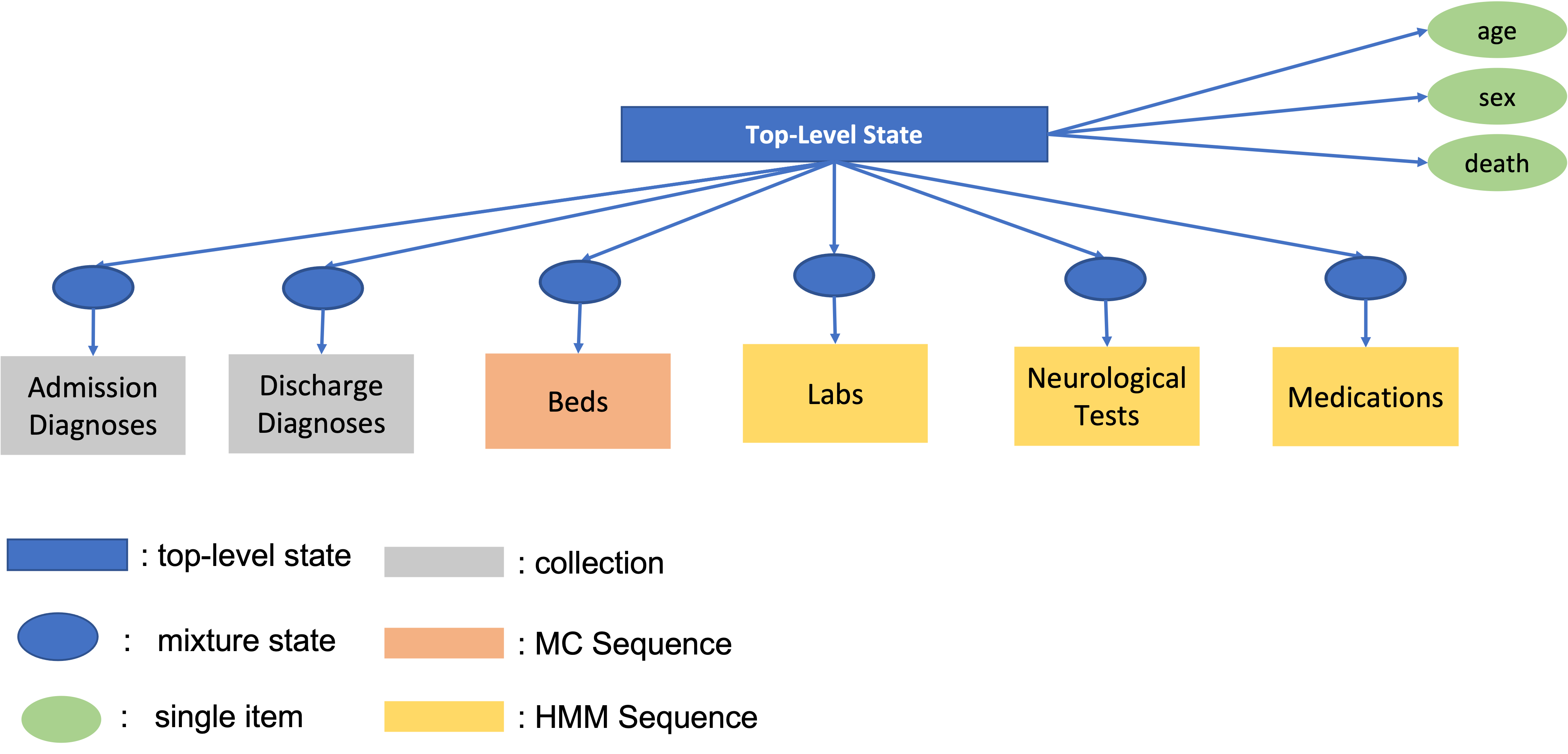
Figure 1: Structure of the model. Arrows indicate dependencies in the model. Blue shapes are latent variables and colors correspond to specific model structure types.

The model consists of a top-layer latent state ($Z$) that links the different data elements and sequences. Under the model, the variables and sequences of an episode are conditionally independent given the latent variable, so that

$$\begin{split}f\left(\boldsymbol{y}|Z=z\right)=&f\left(\phi_{a}|Z=z\right)f\left(\phi_{s}|Z=z\right)f\left(\boldsymbol{\beta}|Z=z\right)f\left(\boldsymbol{\alpha}|Z=z\right)\\ &f\left(\boldsymbol{\delta}|Z=z\right)f\left(\boldsymbol{\lambda}|Z=z\right)f\left(\boldsymbol{\nu}|Z=z\right)f\left(\boldsymbol{\mu}|Z=z\right).\end{split}$$

Each term in this expression is a distribution with learned parameters used to model individual data streams. The distribution of the overall model is formed by summing over the latent variable,

$$f\left(\boldsymbol{y}\right)=\sum_{z}\alpha_{z}f\left(\boldsymbol{y}|Z=z\right),$$

where $\alpha_{z}\geq 0$ is a mixing coefficient such that $\sum_{z}\alpha_{z}=1$. Note that since the latent variable is unknown, the components of the episode are not independent under the model. For example, the likelihood of Age given Sex under this model is $f\left(\phi_{a}|\phi_{s}\right)=\frac{\sum_{z}p_{z}f\left(\phi_{a}|Z=z\right)f\left(\phi_{s}|Z=z\right)}{\sum_{z}p_{z}f\left(\phi_{s}|Z=z\right)}\propto\sum_{z}p_{z}f\left(\phi_{a}|Z=z\right)f\left(Z=z|\phi_{s}\right)$. On the other hand, if the model treated all components to be independent, then this would evaluate to the marginal, $f\left(\phi_{a}\right)$, without considering Sex.

An important aspect of the model is the use of mixture models for the constituent sub-models. This leads to a layered model structure, resulting in a mixture of mixture models. Each sub-model has mixing coefficients dependent on the top-layer component. The model can be interpreted as building up a representation of the multi-sequence data, starting with states for individual sequences at the lower layer. The top layer states captures dependencies between these lower layer states.

Figure 2 shows the sub-model structures used to model the individual data sequences. The colors in this figure correspond to the colors used in Figure 1. Each green circle represents a single data element (e.g., one laboratory result or medication). The sequences can be of differing lengths. In addition, for Laboratory Tests, Neurological Tests, and Medications, the number of items for each timepoint can also vary. The model captures the length of these sequences, as depicted by the # symbol. In this way the model can be trained with sequences of differing and arbitrary lengths. See Appendix A for the generative process describing how episodes can be sampled using the model and Appendix B for a full description of its probability density function.

Collection Model Structure

Admission Diagnoses contain a set of ICD9 codes given at hospital admission, and Discharge Diagnoses contain a set of ICD9 codes given at discharge. For each of these data elements there is no sequence or temporal information, as they occur simultaneously. A mixture is used to capture these sets of codes, where each state contains a probability distribution over sets of codes (see Figure 2a). The number of items (for each state) is described by a Poisson distribution. Within each state, the likelihood of the codes themselves are given by a categorical distribution over the ICD9 codes.

Sequence Model Structures

The Beds, Laboratory Tests, Neurological Tests, and Medications sequences are temporal and have items occurring throughout the hospital stay. For these, we use model structures that distinguish the different collection times, rather than lumping them into one collection. Two distinctions between Beds and the other sequential streams motivate using different sequence model structures. First, only one instance of Beds can occur at a time. And secondly, there are a small number of possible Beds, whereas there are a much larger set of possible items withing the Laboratory Tests, Neurological Tests, and Medications sequences.

The model structure used to describe the Beds sequence is a mixture of Markov chains, where each state contains a Markov chain (see Figure 2b). The length of the sequence is characterized by a Poisson distribution. The Markov chain includes an initial distribution over the set of possible values describing the first item and transition probabilities between sequential items.

For Laboratory Tests, Neurological Tests, and Medications, we use a mixture of Hidden Markov Models (HMMs) (see Figure 2c). Similarly to the Beds model, a Poisson distribution describes the length of the sequence. Within each state of the HMM, multiple items can occur simultaneously. Therefore, each state contains its own length distribution governed by a Poisson rate, and a categorical distribution to describe the collection of items.

Parameter sharing is used to reduce complexity and improve interpretation of the trained model: parameters within the HMM states are shared across mixture states. This leads to an interpretation of a fixed vocabulary that describes each multi-item instance of Laboratory Tests, Neurological Tests, and Medications. The initial and transition probabilities are different across sub-model states to capture a range of different likely sequences.

Top-Layer Latent State

The top-layer latent state selects the subgroup for a patient. Given data, we can infer this variable to compute probabilities of subgroup membership. In addition, mixing coefficients of the underlying mixture models are dependent on the top-layer state. This is a construction of the model. For example, the mixing parameters for the Beds sub-model are $p_{(}\beta,z)$, which is the conditional probability of the Beds state given the top-layer latent variable: $\Pr\left(z_{\beta}|z\right)=p_{\beta,z}$ The same structure is used for all of the sequences. See Appendix A for definitions for the probability distributions and Table 10 for notation of the parameters.

Each of the sub-models have common parameters across the top-level components. For example, the Markov chain parameters for Beds state #2 is the same for all top-layer states. The only parameters that change in this example are the mixing coefficients for the Beds mixture. See Appendices A and B for complete details of the generative model and probability density function. Table 5 summarizes the three types of latent variables included in the model.

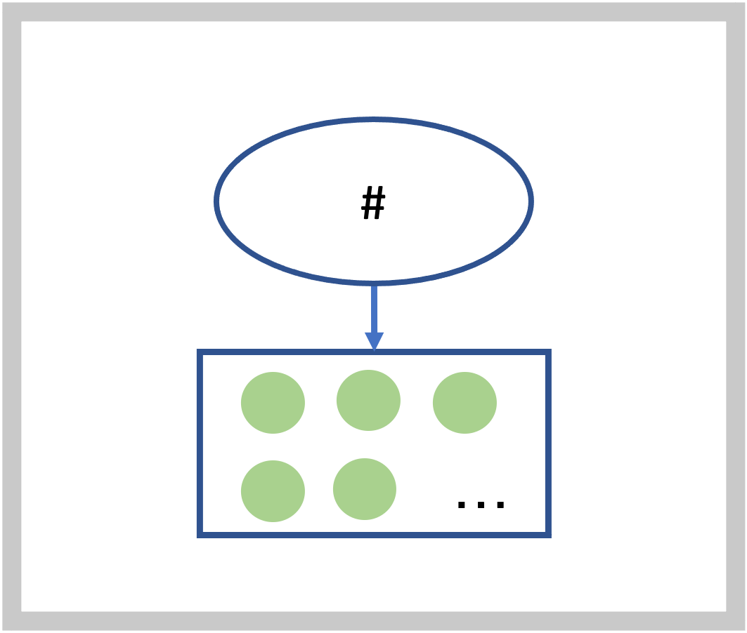
(a) Collection Model

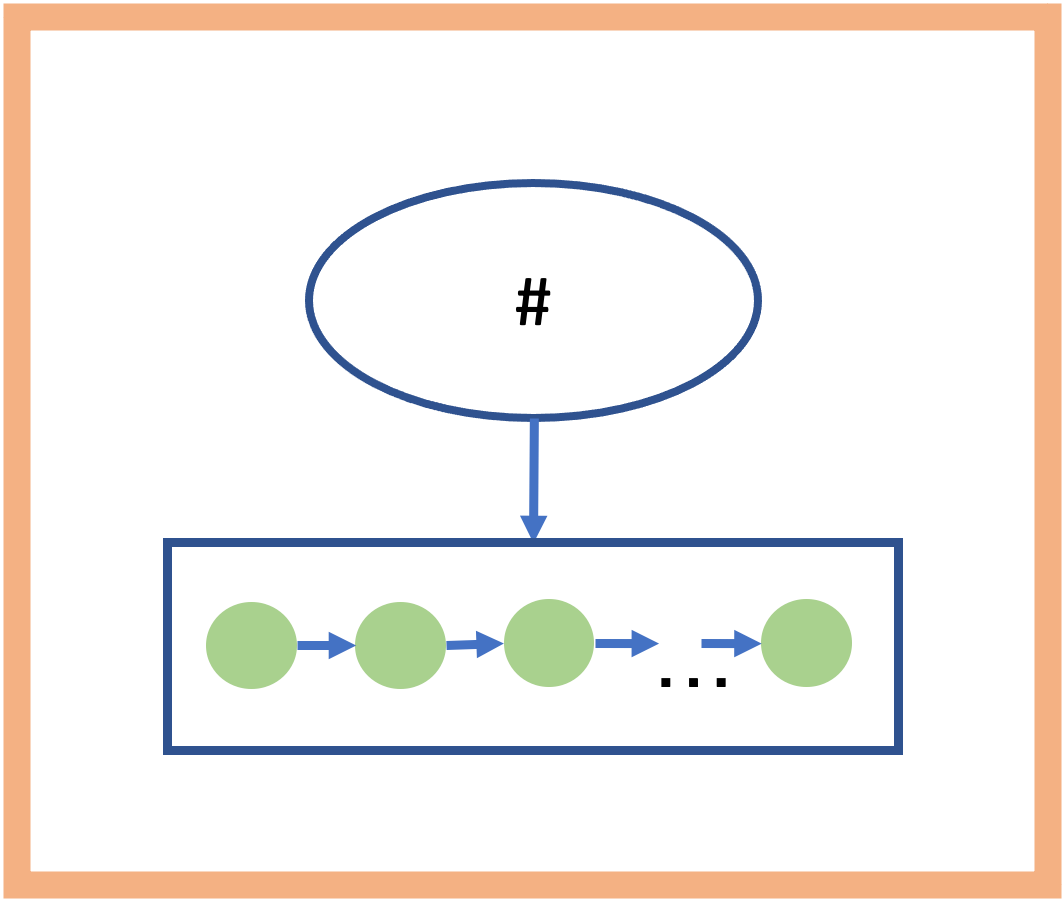
(b) MC Sequence Model

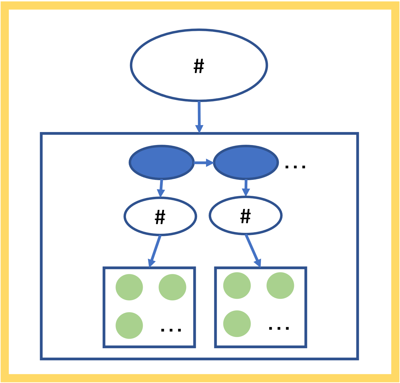
(c) HMM Sequence Model

Figure 2: Three model structures used for the data streams. Admission Diagnoses, Discharge Diagnoses use the collection model (a), Beds use the MC sequence model (b), and Laboratory Results, Medications, and Neurological Tests use the HMM sequence model (c). Colors correspond to those in Figure 1. The # symbols represents the length of the sequence and are captured by Poisson distributions.

Layer	Name	Notation	Data Elements
1	Top-layer states	$z$	All
2	Sub-model states	$z_{\beta},z_{\alpha},z_{\delta},z_{\lambda},z_{\nu},z_{\mu}$	All
3	HMM states	$\boldsymbol{s}_{\lambda},\boldsymbol{s}_{\nu},\boldsymbol{s}_{\mu}$	Laboratory Tests, Neurological Tests, Medications

Table 5: Ontology of Latent States. Each layer contains some number of states in the next lower level.

4 Estimation

The estimation of the model parameters follows the standard Expectation Maximization (EM) procedure, see e.g. [28, 25]. Because the conditional dependence structure is a tree, message passing algorithms can be used to compute the required quantities. Given a set of episodes, $\boldsymbol{y_{1},\ldots,y_{N}}$ we seek to maximize the log-likelihood $\sum_{i=1}^{N}\log\sum_{z}p_{z}f\left(\boldsymbol{y_{i}}|Z=z\right)$. The complete data consists of the episodes, $\boldsymbol{y_{1},\ldots,y_{N}}$, the latent variables, $Z$, $Z_{\alpha}$, $Z_{\delta}$, $Z_{\beta}$, $Z_{\lambda}$, $Z_{\nu}$, $Z_{\mu}$, and the HMM state sequences $\boldsymbol{S}_{\lambda}$, $\boldsymbol{S}_{\nu}$, $\boldsymbol{S}_{\mu}$. We refer to all of the latent variables as $\boldsymbol{Z}$. The complete data log-likelihood is, $\log f\left(\boldsymbol{y},\boldsymbol{Z}\right)=\sum_{i=1}^{N}\sum_{z}I\left(k_{i}=z\right)\left(\log p_{z}+\log f\left(\boldsymbol{y_{i}},\boldsymbol{Z}|Z=z\right)\right),$ where the indicator $I\left(\cdot\right)$ equals 1 when $\cdot$ is true, and otherwise 0. The expected complete data log-likelihood is,

$$\log f\left(\boldsymbol{y},\boldsymbol{Z}\right)=\sum_{i=1}^{N}\sum_{z}\gamma_{i}\left(z\right)\left(\log p_{z}+\mathbb{E}\log f\left(\boldsymbol{y_{i}},\boldsymbol{Z}|Z=z\right)\right),$$

where $\gamma_{i}\left(z\right)=f\left(z|\boldsymbol{y}\right)$. In turn, this likelihood can be written in terms of expected sub-model complete data log-likelihoods,

$$\begin{split}\mathbb{E}\log f\left(\boldsymbol{y_{i}},\boldsymbol{Z}|Z=z\right)&=\sum_{z_{\alpha}}\gamma_{\alpha,i}\left(z_{\alpha}\right)\log f\left(\boldsymbol{\alpha}|Z_{\alpha}=z_{\alpha}\right)\\ &+\sum_{z_{\delta}}\gamma_{\delta,i}\left(z_{\delta}\right)\log f\left(\boldsymbol{\delta}|Z_{\delta}=z_{\delta}\right)\\ &+\sum_{z_{\beta}}\gamma_{\beta,i}\left(z_{\beta}\right)\log f\left(\boldsymbol{\beta}|Z_{\beta}=z_{\beta}\right)\\ &+\sum_{z_{\lambda}}\gamma_{\lambda,i}\left(z_{\lambda}\right)\mathbb{E}\log f\left(\boldsymbol{\lambda},\boldsymbol{S}_{\lambda}|Z_{\lambda}=z_{\lambda}\right)\\ &+\sum_{z_{\nu}}\gamma_{\nu,i}\left(z_{\nu}\right)\mathbb{E}\log f\left(\boldsymbol{\nu},\boldsymbol{S}_{\nu}|Z_{\nu}=z_{\nu}\right)\\ &+\sum_{z_{\mu}}\gamma_{\mu,i}\left(z_{\mu}\right)\mathbb{E}\log f\left(\boldsymbol{\mu},\boldsymbol{S}_{\mu}|Z_{\mu}=z_{\mu}\right),\end{split}$$

where $\gamma_{x,i}\left(z_{x}\right)=f\left(z_{x}|\boldsymbol{y}\right)$ for model $x$. The expected complete data log-likelihoods for $\boldsymbol{\lambda}$, $\boldsymbol{\nu}$, and $\boldsymbol{\mu}$ are the same as for HMMs and are omitted in this description. The EM algorithms proceeds by iterating between calculating gamma and maximizing the expected complete data log-likelihood function.

4.1 Model Selection

In this section, we describe the approach used for model selection. The hyperparameters of the model are:

• the number of top-layer latent states: $|Z|$,

• the number of each sub-model latent states: $|Z_{\alpha}|,|Z_{\delta}|,|Z_{\beta}|,|Z_{\lambda}|,|Z_{\nu}|,|Z_{\mu}|$,

• the number of HMM states: $|\boldsymbol{S}_{\lambda}|,|\boldsymbol{S}_{\nu}|,|\boldsymbol{S}_{\mu}|$.

Note that the number of HMM states is the same across sub-model latent states. This leads to a total of 10 hyperparameters. Model selection is performed using the Bayesian Information Criterion (BIC) as a guide. The BIC penalizes the model fit by a function of the number of parameters: $BIC\left(d\right)=d\ln N-2\ln f\left(\boldsymbol{y}\right)$, where $d$ is the total parameter count and $N$ is the number of episodes. To aid in selecting hyperparameters, we first determine those relating to the lower layers, followed by the top-layer.

To determine these hyperparameters, we first perform linear searches for each sub-model individually. For the mixture of HMM sequence models (Laboratory Tests, Neurological Tests, and Medications), we employ the following strategy:

• Train a sequence of HMMs with increasing state space,

• Compute the BIC for each model, and select the number of HMM states with the lowest corresponding BIC value,

• Train a sequence of mixtures of HMMs with increasing state space using the number of HMM states determined previously,

• Compute the BIC for each model, and select the number of mixture components with the lowest corresponding BIC value.

For the Beds model we perform the following:

• Train a sequence of mixtures of Markov chains with increasing state space,

• Compute the BIC for each model, and select the number of mixture components with the lowest corresponding BIC value.

The collection models (Admission Diagnoses and Discharge Diagnoses) use a similar procedure:

• Train a sequence of collection mixtures with increasing state space,

• Compute the BIC for each model, and select the number of mixture components with the lowest corresponding BIC value.

Once these hyperparameters are determined, we can use them to train the entire model. The number of top-level states can then either be determined again using a linear search over BIC values, or assigned to a pre-selected value. When training the full model, we do not use model parameters determined previously and re-train the entire model, fixing only the hyperparameters.

5 Results

5.1 Training

We used 195,398 episodes to train the model. Following the procedure outlined in Section 4.1, we determined the number of HMM states for the Laboratory Tests, Neurological Tests, and Medications. Then, fixing those hyperparameters, we optimized for the number of mixture states for each sub-model. Both of these were done by searching over every 10 values, e.g., 10, 20, 30, etc. Table 6 shows the optimal number of states found using the model selection approach. To enable more straightforward interpretation of the model, we set the number of top-layer states to 10. We then train all parameters of the final model using these hyperparameters.

Category	Sub-model States	HMM States
Diagnoses	10	N/A
Beds	10	N/A
Laboratory Tests	10	90
Neurological Tests	10	70
Medications	10	40

Table 6: Number of HMM states (for Laboratory Tests, Neurological Tests, and Medications) and mixture states determined by evaluating the BIC score on the training data. The Diagnoses states are shared between Admission Diagnoses and Discharge Diagnoses.

5.2 Top-layer Components with Age, Sex, and Death Probabilities

The top-layer component probabilities are shown in Figure 3(a) in decreasing order. This ordering of the components is preserved throughout the paper. Figures 3(b), 3(c), and 3(d) show learned parameters for scalar variables (Age, Sex, Death) across these 10 components. Components with the highest probability of Death are 4, 5, and 10.

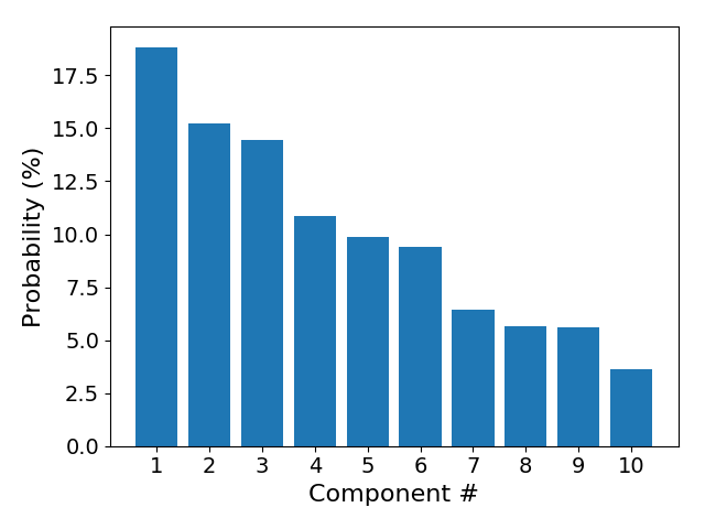
(a) Component Probabilities

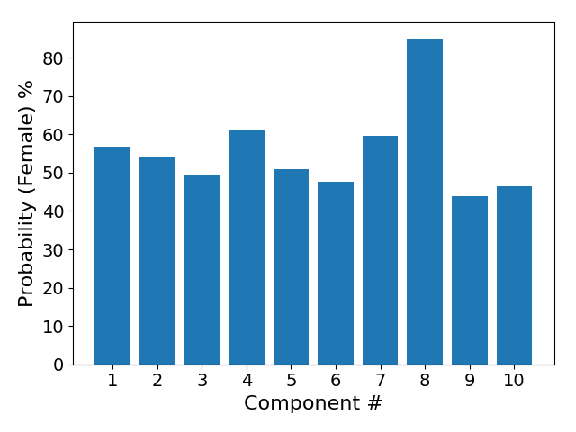
(b) Sex

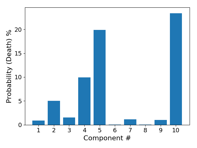
(c) Death

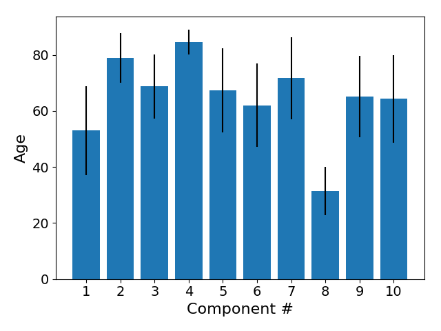
(d) Age

Figure 3: Top-level component probabilities (3(a)), probability of Sex (3(b)), Death (3(c)), and Age mean and spread (3(d)) for each learned component. The components are sorted from highest to lowest probability and correspond across charts.

5.3 Enrichment Analysis- Mortality

Figure 3(c) shows that the probability of Death varies across components. Enrichment of mortality can be defined with respect to each top-layer component. Further, we can determine sub-model states (corresponding to e.g. Beds, Medications, etc.) that are enriched for mortality. This is done by computing

$$f\left(\textsf{Death}|z_{x}\right)\propto\sum_{z}\alpha_{z}f\left(z_{x}|z\right)f\left(\textsf{Death}{}|z\right),$$

where $z$ is the top-layer state and $z_{x}$ is the state for sub-model $x$. This is performed for each sub-model to determine which states have the greatest and least contribution to Death. Table 7 shows the probability of Death given the state for each model.

Sub-Model	1	2	3	4	5	6	7	8	9	10
Beds	0.03	0.08	0.90	4.18	4.43	5.09	8.35	20.72	23.67	32.55
Laboratory Tests	0.10	3.34	3.61	3.66	6.09	6.60	6.61	19.95	24.63	25.38
Neurological Tests	1.22	2.00	2.18	4.46	8.20	8.37	14.20	18.33	20.34	20.70
Medications	0.04	0.08	1.51	2.22	3.12	3.46	5.84	15.84	31.37	36.52

Table 7: Probability of Death (%) for each sub-model state for Beds, Laboratory Tests, Neurological Tests and Medications. States are sorted from lowest to highest probability.

The likelihood of Beds sequences for the lowest Death risk state is shown in Figure 4(a). These sequences are determined from the Markov chain for that state. Probabilities in the tree graph indicate the likelihood of Beds sequences terminating at the corresponding edge. For example, the OB $\rightarrow$ FLR sequence has a likelihood of 15%. Only sequences with likelihood of 1% or greater are shown. Figure 4(b) shows the sequence likelihoods for the highest risk state.

Figures 4(c), 4(d), and 4(e) show the most likely progression through the Laboratory Tests, Neurological Tests, and Medications sequences for the lowest and highest risk states. Each row corresponds to an HMM state, with the three most prevalent items in the first column. Each numbered column represents the time step, and the arrows indicate the most likely sequence through the HMM states for the high and low risk HMM states.

In our trained models, after some number of timepoints, the underlying Hidden Markov Model (HMM) enters an HMM state (rows in Figures 4(c), 4(d), and 4(e)) that has itself as the next most likely HMM state. Thus, for the two risk states considered in the Figure (low and high mortality risk), the models have a terminal HMM state, where it the subject is most likely to remain in. For this reason, we show the initial sequence the states until this phenomenon occurs, after which the most likely HMM state does not change.

For Neurological Tests, Table 4(d) shows the likelihood ratio between Normal and Abnormal results for each Neurological Tests test. Within each cell, the top value is the ratio for the high risk state, and the bottom value is the ratio for the low risk state. Entries with ‘$-$’ indicate that the test is unlikely to be administered (probability $<$ 1%). For example, initially (at timestep 0), Consciousness Level is approximately 25 (1/0.04) times as likely to be normal than abnormal for both the high and low risk groups. At timestep 1, however, abnormal results are 26 times as likely for the high risk state, while the test is unlikely to be administered for the low risk state.

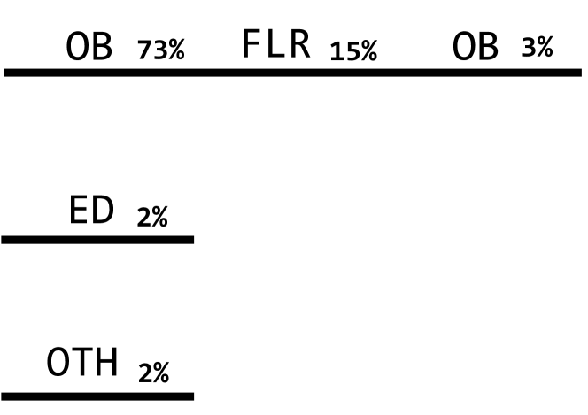
(a)

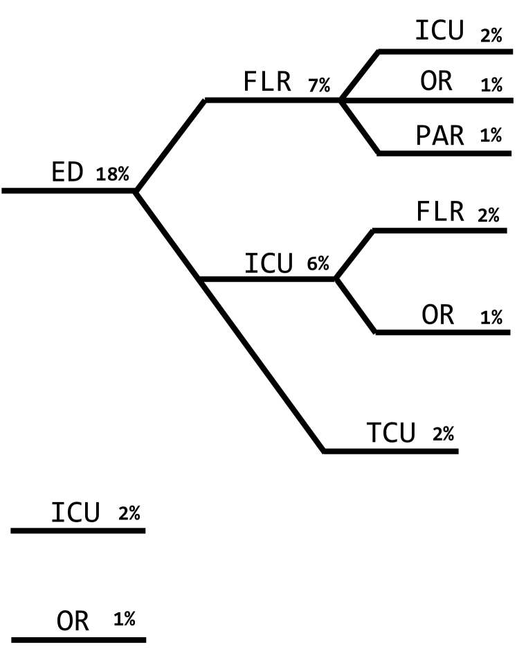
(b)

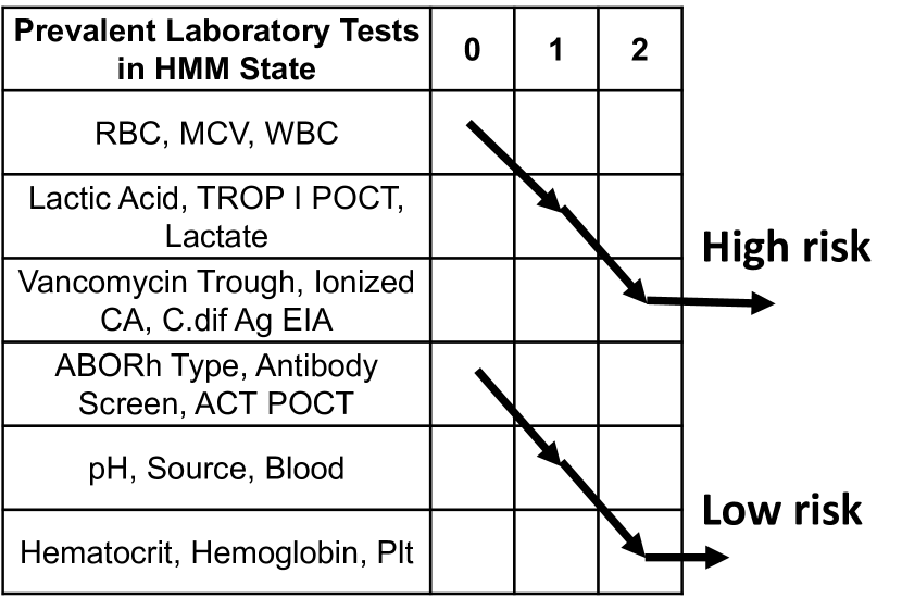
(c)

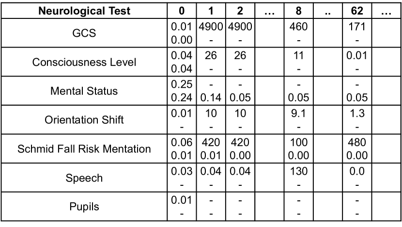
(d)

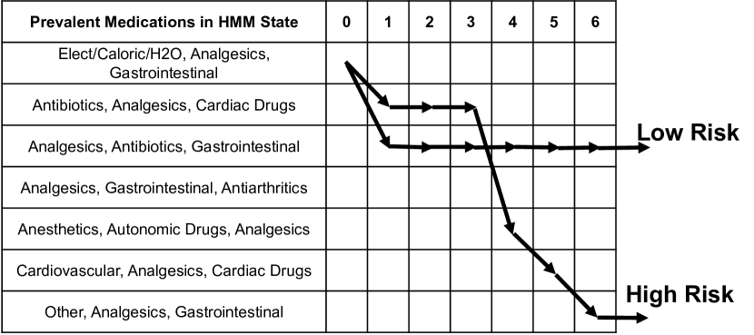
(e)

Figure 4: Lowest and Highest risk states for Death enrichment. Figure 4(a) shows the Beds sequences with the lowest enrichment. Figure 4(b) shows the sequences with the highest enrichment. Figure 4(c) shows the most likely sequences through HMM states for the lowest and highest enrichment. Figure 4(d) shows likelihood ratios for abnormal vs normal Neurological Tests results for the low risk (bottom) and high risk (top) states. Figure 4(e) shows the most likely Medications sequences through he HMM states for the two states.

5.4 Sub-model State Distributions

Figure 5 shows the distributions of the sub-model states for each of the top-layer components. The height of each bar is the probability $\alpha_{z}$ of each component (same as Figure 5). Within each bar are 10 sections, each one corresponding to a sub-model state. The height of these bars are the probabilities of the sub-model state for the given top-layer state, $\alpha_{z}f(z_{x}|z)$. They are ranked and color-coded by the mortality enrichment probabilities computed in Section 5.3, from lowest risk (light red) to highest risk (dark red). Figure 6 shows the state distributions across these 10 components for Admission Diagnoses and Discharge Diagnoses.

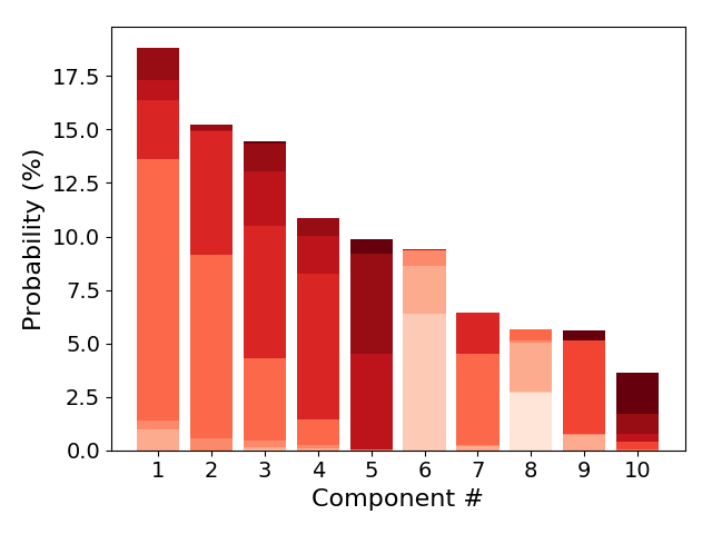
(a) Beds

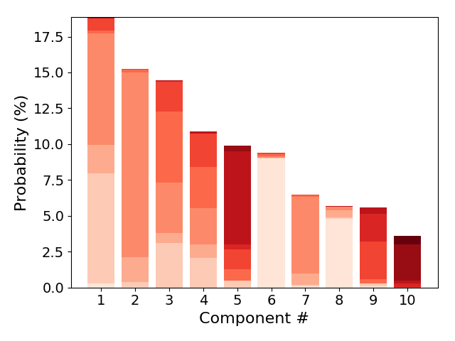
(b) Laboratory Tests

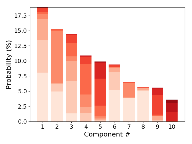
(c) Neurological Tests

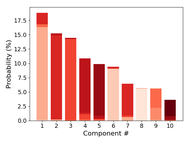
(d) Medications

Figure 5: State distributions across the component states. Each component has a distribution across the 10 underlying states.

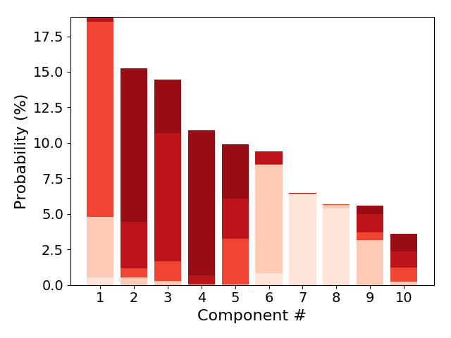
(a) Admission Diagnoses

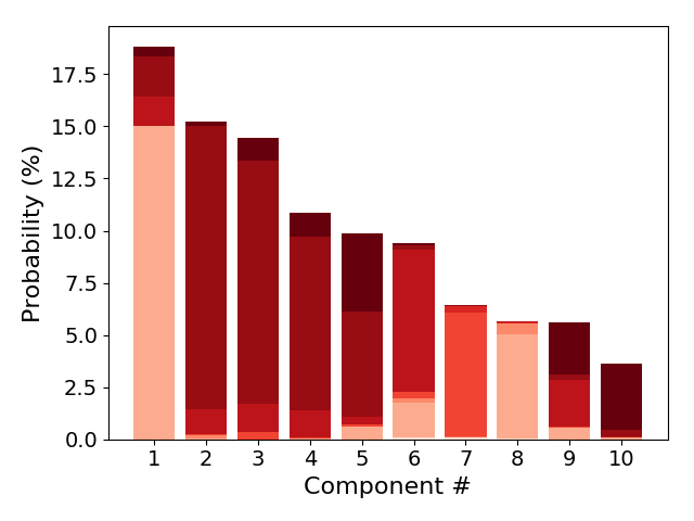
(b) Discharge Diagnoses

Figure 6: Admission Diagnoses and Discharge Diagnoses state distributions across the component states. Each component has a distribution across the 10 underlying states.

5.5 Sequence lengths

The length parameters, which are the mean number (Poisson rate) of items in each state for Beds, Laboratory Tests, Neurological Tests, and Medications are shown in Figure 7. The same color-coding by mortality enrichment is used in these figures as in Figures 5 and 6.

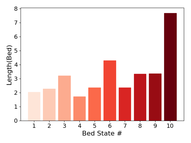
(a)

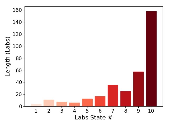
(b)

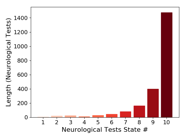
(c)

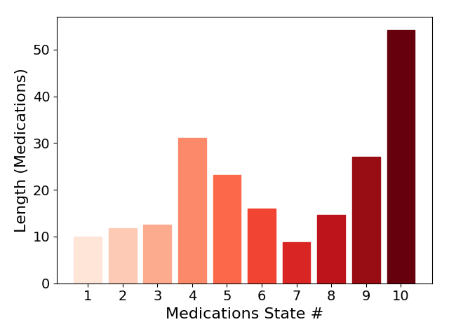
(d)

Figure 7: Learned mean length parameters for the 10 states in each of Beds, Laboratory Tests, Neurological Tests, and Medications. The colors correspond to those in Figure 5.

5.6 Admission Diagnoses and Discharge Diagnoses

Of the 10 states shared across Admission Diagnoses and Discharge Diagnoses, 5 were predominantly associated with Admission Diagnoses and 5 with Discharge Diagnoses. Table 8 shows the 5 most likely ICD9 diagnosis codes for each state associated with Admission Diagnoses. Each column corresponds to a state and column headings contain the prevalence of the state, $\sum_{z}w_{z_{s}}$. The states are sorted in ascending order according to their mortality enrichment. Similarly, Table 9 shows the 5 most likely ICD9 codes for states associated with Discharge Diagnoses.

Diagnosis \Prevalence	13.2%	16.3%	20.6%	19.4%	30.5%
(648.91) Other current conditions classifiable elsewhere of mother, delivered, with or without mention of antepartum condition	X	-	-	-	-
(278.00) Obesity	X	X	-	-	-
(V221) Supervision of other normal pregnancy	X	-	-	-	-
(644.21) Early onset of delivery, delivered, with or without mention of antepartum condition	X	-	-	-	-
(493.90) Asthma	X	-	-	-	-
(401.9) Unspecified essential hypertension	-	X	X	X	X
(272.4) Other and unspecified hyperlipidemia	-	X	X	X	X
(530.81) Esophageal reflux	-	X	X	-	-
(305.1) Tobacco use disorder	-	X	-	-	-
(038.9) Unspecified septicemia	-	-	X	-	-
(995.91) Sepsis	-	-	X	-	-
(250.40) Diabetes with renal manifestations	-	-	-	X	-
(357.2) Polyneuropathy in diabetes	-	-	-	X	-
(403.90) Hypertensive chronic kidney disease	-	-	-	X	X
(427.31) Atrial fibrillation	-	-	-	-	X
(428.0) Congestive heart failure	-	-	-	-	X

Table 8: Most likely (top 5) ICD codes for the states predominantly in Admission Diagnoses. Column headings contain the prevalence of the state.

Diagnosis \Prevalence	22.9%	6.9%	14.7%	41.5%	12.4%
(V15.82) Personal history of tobacco use	X	X	X	X	X
(789.00) Abdominal pain	X	-	-	-	-
(780.60) Fever	X	-	-	-	-
(V27.0) Outcome of delivery, single liveborn	X	-	-	-	-
(682.9) Cellulitis and abscess of unspecified sites	X	-	-	-	-
(272.4) Other and unspecified hyperlipidemia	-	X	-	-	-
(401.9) Unspecified essential hypertension	-	X	-	-	-
(530.81) Esophageal reflux	-	X	-	-	-
(599.0) Urinary tract infection	-	X	-	-	-
(E849.0) Home accidents	-	-	X	-	-
(E849.7) Accidents occurring in residential institution	-	-	X	-	X
(V58.66) Long-term use of aspirin	-	-	X	X	X
(E849.9) Accidents occurring in unspecified place	-	-	X	-	-
(V58.67) Long-term use of insulin	-	-	-	X	X
(V58.61) Long-term use of anticoagulants	-	-	-	X	X
(412) Old myocardial infarction	-	-	-	X	-

Table 9: Most likely (top 5) ICD codes for the states predominantly in Discharge Diagnoses. Column headings contain the prevalence of the state.

5.7 Beds sequences

Beds sequences for each states are shown in Figure 8. Each subfigure is a tree which shows the likelihood of the sequence formed by tracing from the initial bed. This is computed by taking the initial state probabilities and forward simulating the Markov chain for each state. The likelihood of the sequence terminating at a node in the graph is specified in the figures. We stopped once the likelihood dropped below 1%. The states are sorted in ascending order according to their mortality enrichment.

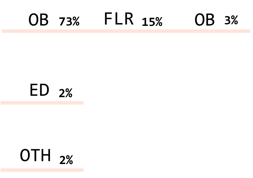
(a) S1

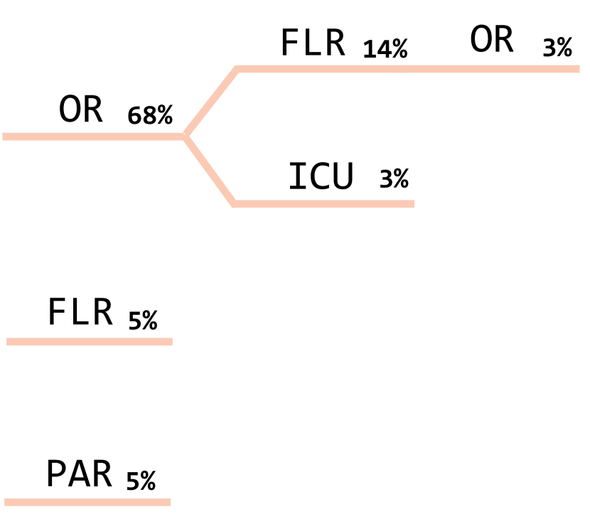
(b) S2

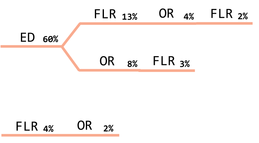
(c) S3

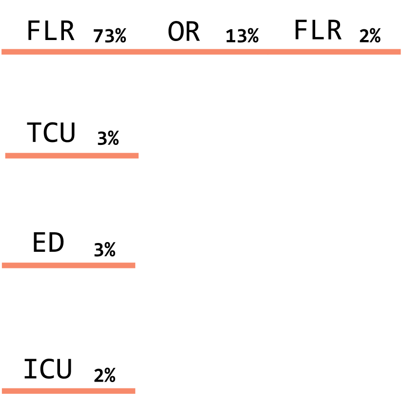
(d) S4

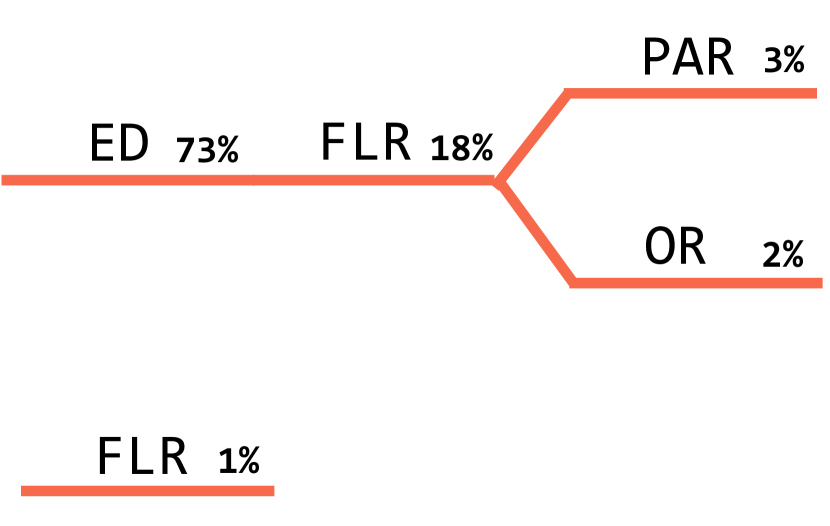
(e) S5

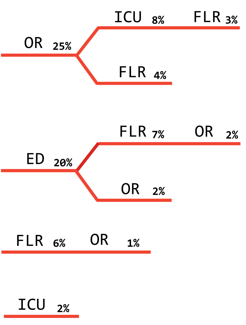
(f) S6

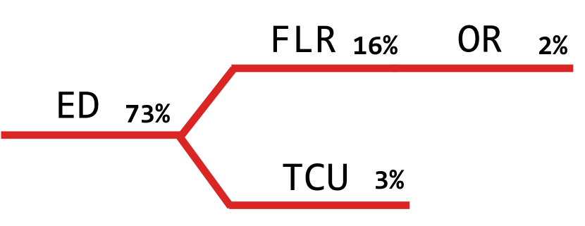
(g) S7

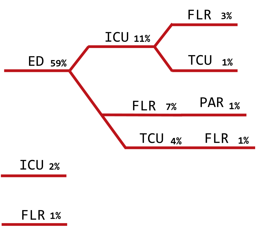
(h) S8

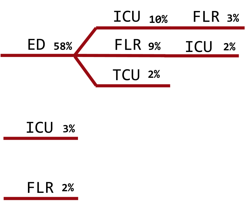
(i) S9

(j) S10

Figure 8: Most likely Beds sequences for each of the Beds states. Likelihoods of the sequences are indicated by the values in the tree graphs. Only sequences with likelihood greater than or equal to 1% are shown. The states are sorted in ascending order according to mortality enrichment.

5.8 Medications sequences

The most likely Medications sequences for are shown in Figure 9. Each row corresponds to an HMM state, with the three most likely therapy classes listed in the first column. Each label column corresponds to a timestep, and arrows through the HMM states over time indicate the most likely sequence for each state. These states are ordered roughly in order of their temporal appearance in these most likely sequences. Colors correspond to the ordering of mortality enrichment by state.

Figure 9: Most likely medication sequences for Medications states. Each row corresponds to an HMM state, showing the three most likely therapy classes for each state.

6 Discussion

The model selection procedure resulted in 10 mixture states for each sequence (Table 6). For the Laboratory Tests, Neurological Tests, and Medications sub-models, the number of HMM states was higher (90, 70, 40, respectively). In our results, we estimated models increasing the number of states by 10 each time. Further granularity would be possible, at higher computational cost.

Distributions of scalar values by top-layer component are shown in Figure 3. The Sex distribution (Figure 3(b)) is fairly consistent around 0.5, with the exception of component 8. Death varies significantly (Figure 3(c)) across components, with the highest probabilities in components 4, 5, and 10. Components 6 and 8 have very low probability of Death. Age profiles also vary (Figure 3(d)), with component 4 having the oldest population with high probability and component 8 having the lowest Age.

Going a layer below these top-layer results, we examine mortality enrichment by computing the likelihood of Death given a sub-model state. This results in 10 likelihoods for each sub-model (Figure 7. States are sorted in increasing order of Death probability. Note that the states are distinct across sub-models (state 1 is not the same state for Beds and Laboratory Tests). These distributions generally start near 0% and rise to 20% - 30%. Generally there is a sharp increase in risk from state S7 to S8, although this is less apparent with Neurological Tests.

Figure 4 characterizes the lowest and highest risk states for Death enrichment. For Beds, the lowest risk state is mostly related to Obstetrics (Figure 4(a)). The highest risk state (Figure 4(b)) is likely to start at the emergency department (ED). The HMM sub-models (Laboratory Tests, Neurological Tests, and Medications) have an additional layer of latent states. The temporal dynamics is described by likelihoods through these HMM states. Likelihood of abnormal Neurological Tests results is generally much higher for the high mortality risk state (Figure 4(d)). The low risk Medications state is most likely to proceed through two states, whereas the high risk state passes through five different states (Figure 4(e)). Note that this is only the single most likely trajectory through the HMMs, and many other state sequences are also possible.

Figure 5 shows how the sub-model states distribute across each top-layer component. These are ranked and color-coded by the mortality risk computed in Section 5.3. The total probability of each component is the component probability $\alpha_{z}$ (same as in Figure 3(a)). It can be seen that components 5 and 10 (highest Death probability) tend to have darker colored states. The same is shown in Figure 6 for Admission Diagnoses and Discharge Diagnoses.

Figures 3 and 5 can be used to link sub-model states with the top layer-components. For example, Figure 3(b) shows that component 8 has the highest likelihood of female Sex. Examining the Beds states that make up this component from Figure 5(a), we see that this component includes the lowest mortality risk state (lightest color). Figure 8(a) shows that OB is a likely visit in this state.

From the mean lengths shown in Figure 7, we can see that for Laboratory Tests and Neurological Tests there is generally an increase in the mean length as the mortality risk increases. The length of the Beds sequence is the number of transitions, rather than an indication of the total time in the hospital. So, if a patient stays in one location (e.g., ICU) for a long time, it will not appear as additional items in the Beds sequence. In the Medications, it may be the case that some mid-risk states receive a large number of Medications (e.g., there are clinical conditions that are not life-threatening, but still require significant extensive medication). In all cases, the highest risk state has the largest length. In general, the states are highly heterogeneous, and we do not necessarily expect a continuous progression of utilization as we progress from low to high mortality risk.

Tables 8 and 9 show the most likely (top 5) ICD codes for Admission Diagnoses and Discharge Diagnoses, respectively. The Admission Diagnoses and Discharge Diagnoses sub-models share the same set of 10 diagnosis states, but only 5 distinct states for each have significant probabilities greater than 0%. These tables show only those 5 states that have significant probabilities. The 5 states in Table 9 for Discharge Diagnoses total 98.4%, so there is a small likelihood of the other states to be in the Discharge Diagnoses. These states are sorted by mortality enrichment. For example, the highest mortality risk Admission Diagnoses state contains Atrial fibrillation and Congestive heart failure in the top 5 codes.

Figures 8 and 9 show the likelihood of Beds and Medications sequences across states, respectively. These are sorted and color coded by mortality risk as well. Note that the states contain probabilistic representations and the results in Figure 9 shows only the most likely trajectory through the HMM state space.

6.1 Limitations

Our model defines the conditional independence between sequences given the top-layer latent state. While it would be possible to extend this method to other structures that do not have this property, doing so may have detrimental consequences. Using our model structure, we are able to control the model complexity by increasing or decreasing the state space of the top-layer latent variable. If instead we directly model interactions between sequences, the parameter count may be too high to enable fine-tuning of the model complexity. In addition, we may find that even second-order statistics between sequences results in a model that does not provide subgrouping properties that are desired. However, there are many other model structures that can be explored.

As described in Section 2, we model the Laboratory Tests, but not the results of the tests. In our modeling framework, it is possible to augment the model with additional sequences. We decided to only model Laboratory Tests because while it would enrich the model, our methodological development would be unaffected. In addition, there is a level of redundancy between the Laboratory Tests, Admission Diagnoses, Discharge Diagnoses, and Medications. The added benefit of including laboratory test results is an open question and application dependent.

In this work, we chose not to include vitals such as heart-rate and respiratory-rate. Although it is possible to include vitals as another sequence, they were left out because they are often sampled at a high rate and would require significant additional model training. In general, there are many sources of data that could be incorporated. We had to make a decision to include enough data that can generate interesting results, while not overburdening our computational resources while developing this novel methodology.

An aspect of the data that is not captured by our model is the explicit time-dependence. We do incorporate sequence order for Beds and Medications sequences, but the distribution of time point is not captured. This can be accomplished in a number of different ways, ranging from modeling the average arrival times (for example, with Exponential distributions) to full time-dependent sequence models. Additional model complexity comes at the cost of requiring more data, and the choice should depend on the specific application at hand.

Our model is geared towards characterizing episodic sequences, rather than patient-centric modeling for following patient trajectories over time. It assumes that each episode is drawn independently from the model, even when the same individual has 2 episodes. Repeat episodes from the same individual may have differing characteristics from the initial episode. Also, our data are selected from a specific timeframe, and are not guaranteed to have all episodes for any given subject. However, the model as developed can capture differing characteristics between initial and repeat visits. In addition, it is possible that specific mixture components are more representative of repeat visits This analysis, and the inclusion of additional parameters to link episodes, however, is beyond the scope of this work.

7 Conclusions

In this work we formulated a statistical model for sequences of varying length, as commonly found in EHR data. An important characteristic of the model is a layered set of latent variables. The top-layer latent variable controls dependence between the sequences, and can be interpreted as a subject subgroup indicator. Sub-model states express subgroupings in the sequence space. Having both layers of latent variables provides an intuitive way of explored the trained model, through subgroups of subjects and subgroups of likely sequences. The intersection of these subgroups can be examined to uncover phenotypes for specific conditions of interest. Sequence lengths are explicitly modeled through Poisson distributions, enabling us to distinguish sequences of varying lengths. We trained the model using EHR data and explored its internal representations through probability distributions.

The purpose of the method developed in this work is a general model capable of subgrouping and subtyping for heterogeneous sequence EHR data. In addition to uncovering patterns in the data, this approach can be used to study disease phenotypes, since relationships between hospitalization data and certain disease states are included in the model. To the extent that disease states are captured by diagnosis codes, this can be seen in our results relative to admission and discharge diagnosis codes (Section 5.6, Table 8, and Table 9). For example, there are specific diagnosis states where Sepsis or Polyneuropathy in diabetes are most common. These could then be traced back through the top-level components to determine likely trajectories of the other sequences (e.g., Beds, Laboratory Tests, etc.) that are most likely to be linked with the disease.

We perform such an analysis for mortality (Section 5.3 and Figure 4), where the probability of Death is computed for each top-layer state and related to underlying sequences sub-models. For these analyses, however, we are using a separate variable (Death) to perform the analysis. In general, the model could be augmented to incorporate variables describing a particular disease state of interest. In that case, this analysis can be performed to learn phenotypes for the disease.

Using and applying this method is dependent on the data types being modeled and the computational resources necessary to train the model. For sequence types that differ in format significantly from the ones we consider in this work, corresponding sub-model structures would need to be implemented. The computational resources required are primarily for training the model. Once trained, modest resources are required to perform subgroup analysis and inference.

As the ability to integrate heterogeneous data streams is an important aspect of precision medicine, we believe that this methodology hold promise towards the development of decision support systems. Using data from Kaiser Permanente Northen California, we have shown how the models described can be used to subgroup patients and interpret these subgroups based on likely trajectories of data elements such as Laboratory Tests, Medications, and Beds. Such patterns are often difficult to uncover because they are hidden within long sequences. We showed how we can analyze sequences that contribute to the assessment of mortality risk. In future work, this inference can be expanded to other areas, such as risk of disease, or length of hospital stay. Also, since the model is a full likelihood function of the data, conditional probabilities can be computed between any subsets of the sequences to flexibly infer future sequence values.

8 Acknowledgments

This work was performed under the auspices of the U.S. Department of Energy by Lawrence Livermore National Laboratory under Contract DE-AC52-07NA27344 and was supported by the LLNL LDRD Program under Project 19-ERD-009. VXL was supported in part by NIH R35GM128672.

Appendix A Generative Description

The generative picture hinges on an underlying and unobserved state $z$. Under the model an episode $\boldsymbol{y}$ may be sampled by performing the following:

• Draw a state $z$ from a categorical distribution: $z\sim Categorical\left(\boldsymbol{p}\right)$

• Draw an Age using a quantized Gaussian distribution, conditioned on the top-layer state: $\phi_{a}\sim\mathcal{N}_{q}\left(\mu_{z},\sigma_{z}^{2}\right)$

• Draw the Sex using a Bernoulli distribution conditioned on the top-layer state: $\phi_{s}\sim Bern\left(p_{s,z}\right)$

• Draw the Death flag using a Bernoulli distribution conditioned on the top-layer state: $\phi_{d}\sim Bern\left(p_{d,z}\right)$

• Draw the Beds sub-model latent state from a categorical distribution, conditional on the top-layer state: $z_{\beta}\sim Categorical\left(\boldsymbol{p}_{\beta,z}\right)$

  • Draw the number of Beds from a Poisson distribution, conditioned on the state: $k_{\beta}\sim Poisson\left(l_{\beta,z_{\beta}}\right)$

  • Draw $k_{\beta}$ Beds from a Markov Chain, conditioned on the state: $\boldsymbol{\beta}\sim MarkovChain\left(\boldsymbol{p}_{\beta,z_{\beta}},\boldsymbol{q}_{\beta,z_{\beta}}\right)$

• Draw the Admission Diagnoses sub-model state from a categorical distribution, conditioned on the state: $z_{\alpha}\sim Categorical\left(\boldsymbol{p}_{\alpha,z}\right)$

  • Draw the number of Admission Diagnoses from a Poisson distribution, conditioned on the state: $k_{\alpha}\sim Poisson\left(l_{\alpha,z_{\alpha}}\right)$

  • Draw $k_{\alpha}$ Admission Diagnoses by taking repeated draws from a categorical distribution, conditioned on the state: $\boldsymbol{\alpha}\sim Categorical\left(\boldsymbol{p}_{D,z_{\alpha}}\right)$

• Draw the Discharge Diagnoses sub-model state from a categorical distribution, conditioned on the state: $z_{\delta}\sim Categorical\left(\boldsymbol{p}_{\delta,z}\right)$

  • Draw the number of Discharge Diagnoses from a Poisson distribution, conditioned on the state: $k_{\delta}\sim Poisson\left(l_{\delta,z_{\delta}}\right)$

  • Draw $k_{\delta}$ Discharge Diagnoses by taking repeated draws from a categorical distribution, conditioned on the state: $\boldsymbol{\delta}\sim Categorical\left(\boldsymbol{p}_{D,z_{\delta}}\right)$

• Draw the Laboratory Tests sub-model state from a categorical distribution, conditioned on the state: $z_{\lambda}\sim Categorical\left(\boldsymbol{p}_{\lambda,z}\right)$

  • Draw the number of distinct Laboratory Tests instances from a Poisson distribution, conditioned on the state: $k_{\lambda}\sim Poisson\left(l_{\lambda,z_{\lambda}}\right)$

  • Draw a Laboratory Tests HMM state sequence from a Markov Chain: $\boldsymbol{s}_{\lambda}\sim MarkovChain\left(\boldsymbol{p}_{\lambda,z_{\lambda}},\boldsymbol{q}_{\lambda,z_{\lambda}}\right)$

  • Draw the number of Laboratory Tests given for each instance from a Poisson distribution, conditioned on the state: $k_{\lambda,s_{\lambda}}\sim Poisson\left(l_{L,s_{\lambda}}\right)$

  • Draw a set of $k_{\lambda,s_{\lambda}}$ Laboratory Tests for each instance by taking repeated draws of a Categorical distribution, conditioned on the state: $\boldsymbol{\lambda}_{s_{\lambda}}\sim Categorical\left(\boldsymbol{p}_{L,s_{\lambda}}\right)$

• Draw the Neurological Tests sub-model state from a categorical distribution, conditioned on the state: $z_{\nu}\sim Categorical\left(\boldsymbol{p}_{\nu,z}\right)$

  • Draw the number of distinct Neurological Tests instances from a Poisson distribution, conditioned on the state: $k_{\nu}\sim Poisson\left(l_{\nu,z_{\nu}}\right)$

  • Draw a Neurological Tests HMM state sequence from a Markov Chain: $\boldsymbol{s}_{\nu}\sim MarkovChain\left(\boldsymbol{p}_{\nu,z_{\nu}},\boldsymbol{q}_{\nu,z}\right)$

  • Draw the number of Neurological Tests given for each instance from a Poisson distribution, conditioned on the state: $k_{\nu,s_{\nu}}\sim Poisson\left(l_{N,s_{\nu}}\right)$

  • Draw a set of $k_{\nu,s_{\nu}}$ Neurological Tests for each instance by taking repeated draws of a Categorical distribution, conditioned on the state: $\boldsymbol{\nu}_{s_{\nu}}\sim Categorical\left(\boldsymbol{p}_{N,s_{\nu}}\right)$

• Draw the Medications sub-model state from a categorical distribution, conditioned on the state: $z_{\mu}\sim Categorical\left(\boldsymbol{p}_{\mu,z}\right)$

  • Draw the number of distinct Medications instances from a Poisson distribution, conditioned on the state: $k_{\mu}\sim Poisson\left(l_{\mu,z_{\mu}}\right)$

  • Draw a Medications HMM state sequence from a Markov Chain: $\boldsymbol{s}_{\mu}\sim MarkovChain\left(\boldsymbol{p}_{\mu,z_{\mu}},\boldsymbol{q}_{\mu,z_{\mu}}\right)$

  • Draw the number of Medications given for each instance from a Poisson distribution, conditioned on the state: $k_{\mu,s_{\mu}}\sim Poisson\left(l_{M,s_{\mu}}\right)$

  • Draw a set of $k_{\mu,s_{\mu}}$ Medications for each instance by taking repeated draws of a Categorical distribution, conditioned on the state: $\boldsymbol{\mu}_{s}\sim Categorical\left(\boldsymbol{p}_{M,s_{\mu}}\right)$

Appendix B Probability Density Functions

For Age, we use a quantized and truncated Gaussian distribution. This conditional distribution is,

$$f\left(\phi_{a}|Z=z\right)=\frac{1}{C\sqrt{2\pi\sigma_{z}^{2}}}e^{\frac{\left(m_{z}-\phi_{a}\right)^{2}}{2\sigma_{z}^{2}}},$$

where the normalizing value ensures that the distribution sums to 1, $C=\sum_{\phi_{a}}\frac{1}{\sqrt{2\pi\sigma_{z}^{2}}}e^{\frac{\left(m_{z}-\phi_{a}\right)^{2}}{2\sigma_{z}^{2}}}$.

For Sex and Death, we we use Bernoulli distributions,

$$f\left(\phi_{s}|Z=z\right)=p_{s,z}^{1-\phi_{s}}\left(1-p_{s,z}\right)^{\phi_{s}},$$

$$f\left(\phi_{d}|Z=z\right)=p_{d,z}^{1-\phi_{d}}\left(1-p_{d,z}\right)^{\phi_{d}}.$$

For the Beds sequence we use a mixture of Markov chains, where the length of the sequence is captured by Poisson distribution. The distribution is,

$$f\left(\boldsymbol{\beta}|Z=z\right)=\sum_{z_{\beta}}p_{z,z_{\beta}}\frac{l_{z_{\beta}}^{|\boldsymbol{\beta}|}}{|\boldsymbol{\beta}|!}e^{-l_{\beta,z_{\beta}}}p_{\beta,z_{\beta},\beta_{1}}\prod_{i=1}^{|\boldsymbol{\beta}|-1}q_{\beta,z_{\beta},\beta_{i},\beta_{i+1}},$$

where $p_{\beta,z_{\beta},i}$ is the probability that the first item is $i$ conditioned on $Z_{\beta}=z_{\beta}$, and $q_{\beta,z_{\beta},i,j}$ is the probability of transitioning from item $i$ to $j$ conditioned on $Z\beta=z_{\beta}$.

For Admission Diagnoses and Discharge Diagnoses we use mixtures over products of categorical distributions. The length of each of these sequences for the entire episode ($|\boldsymbol{\alpha}|$ for Admission Diagnoses and $|\boldsymbol{\delta}|$ for Discharge Diagnoses) is modeled using a Poisson distribution. For these sets we have,

$$f\left(\boldsymbol{\alpha}|Z=z\right)=\sum_{z_{\alpha}}p_{z,z_{\alpha}}\frac{l_{\alpha,z_{\alpha}}^{|\boldsymbol{\alpha}|}}{|\boldsymbol{\alpha}|!}e^{-l_{\alpha,z_{\alpha}}}\prod_{i=1}^{|\boldsymbol{\alpha}|}p_{\alpha,z_{\alpha},\alpha_{i}},$$

$$f\left(\boldsymbol{\delta}|Z=z\right)=\sum_{z_{\delta}}p_{z,z_{\delta}}\frac{l_{\delta,z_{\delta}}^{|\boldsymbol{\delta}|}}{|\boldsymbol{\delta}|!}e^{-l_{\delta,z_{\delta}}}\prod_{i=1}^{|\boldsymbol{\delta}|}p_{\delta,z_{\delta},\delta_{i}},$$

where $p_{x,z_{\alpha},i}$ is the probability of item $i$ in sequence $x$ for sub-model latent state $z_{\alpha}$, and $p_{x,z_{\delta},i}$ is the probability of item $i$ in sequence $x$ for sub-model latent state $z_{\delta}$

The Laboratory Tests, Neurological Tests, and Medications sub-models can have multiple items at any timepoint. This is modeled using HMMs, where where the HMM transitions there a latent state sequence, $\boldsymbol{S}$, over time. Each state can have any number of observations, drawn from a categorical distribution. The number of observations is captured with a Poisson distribution conditioned on the state. In this way we are able to model the ordered sequence and express multiple simultaneous observations. A mixture of these HMM models is used for the Laboratory Tests, Neurological Tests, and Medications observations. This distributions for these are,

$$f\left(\boldsymbol{\lambda}|Z=z\right)=\sum_{z_{\lambda}}p_{z,z_{\lambda}}\frac{l_{\lambda,z_{\lambda}}^{|\boldsymbol{\lambda}|}}{|\boldsymbol{\lambda}|!}e^{-l_{\lambda,z_{\lambda}}}\sum_{\boldsymbol{S}}\left(p_{\lambda,z_{\lambda},s_{1}}\prod_{i=1}^{|\boldsymbol{\lambda}|-1}q_{\lambda,z_{\lambda},s_{i},s_{i+1}}\right)\left(\prod_{i=1}^{|\boldsymbol{\lambda}|}\frac{l_{\lambda,z_{\lambda},s_{i}}^{|\boldsymbol{\lambda}_{i}|}}{|\boldsymbol{\lambda}_{i}|!}e^{-l_{\lambda,z_{\lambda},s_{i}}}\prod_{j=1}^{|\boldsymbol{\lambda}_{i}|}p_{\lambda,z_{\lambda},s_{i},\lambda{i,j}}\right),$$

$$f\left(\boldsymbol{\nu}|Z=z\right)=\sum_{z_{\nu}}p_{z,z_{\nu}}\frac{l_{\nu,z_{\nu}}^{|\boldsymbol{\nu}|}}{|\boldsymbol{\nu}|!}e^{-l_{\nu,z_{\nu}}}\sum_{\boldsymbol{S}}\left(p_{\nu,z_{\nu},s_{1}}\prod_{i=1}^{|\boldsymbol{\nu}|-1}q_{\nu,z_{\nu},s_{i},s_{i+1}}\right)\left(\prod_{i=1}^{|\boldsymbol{\nu}|}\frac{l_{\nu,z_{\nu},s_{i}}^{|\boldsymbol{\nu}_{i}|}}{|\boldsymbol{\nu}_{i}|!}e^{-l_{\nu,z_{\nu},s_{i}}}\prod_{j=1}^{|\boldsymbol{\nu}_{i}|}p_{\nu,z_{\nu},s_{i},\nu{i,j}}\right),$$

$$f\left(\boldsymbol{\mu}|Z=z\right)=\sum_{z_{\mu}}p_{z,z_{\mu}}\frac{l_{\mu,z_{\mu}}^{|\boldsymbol{\mu}|}}{|\boldsymbol{\mu}|!}e^{-l_{\mu,z_{\mu}}}\sum_{\boldsymbol{S}}\left(p_{\mu,z_{\mu},s_{1}}\prod_{i=1}^{|\boldsymbol{\mu}|-1}q_{\mu,z_{\mu},s_{i},s_{i+1}}\right)\left(\prod_{i=1}^{|\boldsymbol{\mu}|}\frac{l_{\mu,z_{\mu},s_{i}}^{|\boldsymbol{\mu}_{i}|}}{|\boldsymbol{\mu}_{i}|!}e^{-l_{\mu,z_{\mu},s_{i}}}\prod_{j=1}^{|\boldsymbol{\mu}_{i}|}p_{\mu,z_{\mu},s_{i},\mu_{i,j}}\right),$$

where $p_{z,z_{\lambda}}$ is the probability of sub-model state $z_{\lambda}$ given the top-layer state $z$, $p_{\lambda,z_{\lambda},i}$ is the probability that state $i$ is the initial state, $q_{\lambda,z_{\lambda},i,j}$ is the transition probability from HMM state $i$ to HMM state $j$, and $p_{\lambda,z_{\lambda},i,j}$ is the probability of medication $j$ conditioned on HMM state $i$ and sub-model state $z_{\lambda}$. And the same holds (substituting $\nu$ or $\mu$ for $\lambda$) for the Neurological Tests and Medications models.

The complete set of parameters is shown in Table 10, along with the number of parameters in each category. In this Table, $|Z|$ is the number of top-layer latent states, $|Z_{x}|$ is the number of sub-model latent states for model $x$, $\mathcal{C}_{x}$ is the number of possible items in $x$. The number of HMM states is $\mathcal{C}_{S,x}$ for HMM model $x$.

Data Element	Parameters	Count
Top-layer latent state $Z$	$p_{z}$	$|Z|$
Admission Diagnoses latent state $Z_{\alpha}$	$p_{z,z_{\alpha}}$	$|Z|\times|Z_{\alpha}|$
Discharge Diagnoses latent state $Z_{\delta}$	$p_{z,z_{\delta}}$	$|Z|\times|Z_{\delta}|$
Beds latent state $Z_{\beta}$	$p_{z,z_{\beta}}$	$|Z|\times|Z_{\beta}|$
Laboratory Tests latent state $Z_{\lambda}$	$p_{z,z_{\lambda}}$	$|Z|\times|Z_{\lambda}|$
Neurological Tests latent state $Z_{\nu}$	$p_{z,z_{\nu}}$	$|Z|\times|Z_{\nu}|$
Medications latent state $Z_{\mu}$	$p_{z,z_{\mu}}$	$|Z|\times|Z_{\mu}|$
Age	$m_{z},\sigma_{z}^{2}$	$2|Z|$
Sex	$p_{s,z}$	$|Z|$
Death	$p_{d,z}$	$|Z|$
Admission Diagnoses	$l_{\alpha,z_{\alpha}},p_{\alpha,z_{\alpha},i}$	$\left(1+\mathcal{C}_{\alpha}\right)|Z_{\alpha}|$
Discharge Diagnoses	$l_{\delta,z_{\delta}},p_{\delta,z_{\delta},i}$	$\left(1+\mathcal{C}_{\delta}\right)|Z_{\delta}|$
Beds	$l_{\beta,z_{\beta}},p_{\beta,z_{\beta},i},q_{\beta,z_{\beta},i,j}$	$\left(1+\mathcal{C}_{\beta}+\mathcal{C}_{\beta}^{2}\right)|Z_{\beta}|$
Laboratory Tests	$l_{\lambda,z_{\lambda}},p_{\lambda,z_{\lambda},i},q_{\lambda,z_{\lambda},i,j},p_{\lambda,z_{\lambda},s,i}$	$\left(1+\mathcal{C}_{S,\lambda}+\mathcal{C}_{S,\lambda}^{2}+\mathcal{C}_{S,\lambda}\mathcal{C}_{\lambda}\right)|Z_{\lambda}|$
Neurological Tests	$l_{\nu,z_{\nu}},p_{\nu,z_{\nu},i},q_{\nu,z_{\nu},i,j},p_{\nu,z_{\nu},s,i}$	$\left(1+\mathcal{C}_{S,\nu}+\mathcal{C}_{S,\nu}^{2}+\mathcal{C}_{S,\nu}\mathcal{C}_{\nu}\right)|Z_{\nu}|$
Medications	$l_{\mu,z_{\mu}},p_{\mu,z_{\mu},i},q_{\mu,z_{\mu},i,j},p_{\mu,z_{\mu},s,i}$	$\left(1+\mathcal{C}_{S,\mu}+\mathcal{C}_{S,\mu}^{2}+\mathcal{C}_{S,\mu}\mathcal{C}_{\mu}\right)|Z_{\mu}|$

Table 10: Model parameters for each data element and the parameter count.

References

- Alaa and van der Schaar [2017] Alaa, A.M., van der Schaar, M., 2017. Bayesian inference of individualized treatment effects using multi-task gaussian processes. Adv. Neural Inf. Process. Syst. 30.
- Alaa et al. [2018] Alaa, A.M., Yoon, J., Hu, S., van der Schaar, M., 2018. Personalized risk scoring for critical care prognosis using mixtures of gaussian processes. IEEE Trans. Biomed. Eng. 65, 207–218.
- Barak-Corren et al. [2017] Barak-Corren, Y., Castro, V.M., Javitt, S., Hoffnagle, A.G., Dai, Y., Perlis, R.H., Nock, M.K., Smoller, J.W., Reis, B.Y., 2017. Predicting suicidal behavior from longitudinal electronic health records. Am. J. Psychiatry 174, 154–162.
- Cheung et al. [2017] Cheung, L.C., Pan, Q., Hyun, N., Schiffman, M., Fetterman, B., Castle, P.E., Lorey, T., Katki, H.A., 2017. Mixture models for undiagnosed prevalent disease and interval-censored incident disease: applications to a cohort assembled from electronic health records. Stat. Med. 36, 3583–3595.
- Choi et al. [2016] Choi, E., Bahadori, M.T., Schuetz, A., Stewart, W.F., Sun, J., 2016. Doctor AI: Predicting clinical events via recurrent neural networks. JMLR Workshop Conf. Proc. 56, 301–318.
- Cui et al. [2022] Cui, S., Yoo, E.C., Li, D., Laudanski, K., Engelhardt, B.E., 2022. Hierarchical gaussian processes and mixtures of experts to model COVID-19 patient trajectories. Pac. Symp. Biocomput. 27, 266–277.
- Futoma et al. [2017] Futoma, J., Hariharan, S., Heller, K., 2017. Learning to detect sepsis with a multitask gaussian process RNN classifier, in: International Conference on Machine Learning, proceedings.mlr.press. pp. 1174–1182.
- Ghahramani [2015] Ghahramani, Z., 2015. Probabilistic machine learning and artificial intelligence. Nature 521, 452–459.
- Ginsburg and Phillips [2018] Ginsburg, G.S., Phillips, K.A., 2018. Precision medicine: From science to value. Health Aff. 37, 694–701.
- Huang et al. [2018] Huang, Z., Ge, Z., Dong, W., He, K., Duan, H., 2018. Probabilistic modeling personalized treatment pathways using electronic health records. J. Biomed. Inform. 86, 33–48.
- Hubbard et al. [2017] Hubbard, R.A., Johnson, E., Chubak, J., Wernli, K.J., Kamineni, A., Bogart, A., Rutter, C.M., 2017. Accounting for misclassification in electronic health records-derived exposures using generalized linear finite mixture models. Health Serv. Outcomes Res. Methodol. 17, 101–112.
- Jin et al. [2018] Jin, B., Che, C., Liu, Z., Zhang, S., Yin, X., Wei, X., 2018. Predicting the risk of heart failure with EHR sequential data modeling. IEEE Access 6, 9256–9261.
- Kam and Kim [2017] Kam, H.J., Kim, H.Y., 2017. Learning representations for the early detection of sepsis with deep neural networks. Comput. Biol. Med. 89, 248–255.
- Kim et al. [2019] Kim, E., Rubinstein, S.M., Nead, K.T., Wojcieszynski, A.P., Gabriel, P.E., Warner, J.L., 2019. The evolving use of electronic health records (EHR) for research. Semin. Radiat. Oncol. 29, 354–361.
- Kosorok and Laber [2019] Kosorok, M.R., Laber, E.B., 2019. Precision medicine. Annu. Rev. Stat. Appl. 6, 263–286.
- Levine et al. [2018] Levine, M.E., Albers, D.J., Hripcsak, G., 2018. Methodological variations in lagged regression for detecting physiologic drug effects in EHR data. J. Biomed. Inform. 86, 149–159.
- Li et al. [2016] Li, C., Rana, S., Phung, D., Venkatesh, S., 2016. Hierarchical bayesian nonparametric models for knowledge discovery from electronic medical records. Knowl. Based Syst. 99, 168–182.
- Li et al. [2021] Li, Y., Rao, S., Hassaine, A., Ramakrishnan, R., Canoy, D., Salimi-Khorshidi, G., Mamouei, M., Lukasiewicz, T., Rahimi, K., 2021. Deep bayesian gaussian processes for uncertainty estimation in electronic health records. Sci. Rep. 11, 20685.
- Liu et al. [2016] Liu, S., Liu, H., Chaudhary, V., Li, D., 2016. An infinite mixture model for coreference resolution in clinical notes. AMIA Jt Summits Transl Sci Proc 2016, 428–437.
- Liu et al. [2017] Liu, V.X., Fielding-Singh, V., Greene, J.D., Baker, J.M., Iwashyna, T.J., Bhattacharya, J., Escobar, G.J., 2017. The timing of early antibiotics and hospital mortality in sepsis. Am. J. Respir. Crit. Care Med. 196, 856–863.
- Liu et al. [2015] Liu, Y.Y., Li, S., Li, F., Song, L., Rehg, J.M., 2015. Efficient learning of Continuous-Time hidden markov models for disease progression. Adv. Neural Inf. Process. Syst. 28, 3599–3607.
- Luz et al. [2020] Luz, C.F., Vollmer, M., Decruyenaere, J., Nijsten, M.W., Glasner, C., Sinha, B., 2020. Machine learning in infection management using routine electronic health records: tools, techniques, and reporting of future technologies. Clin. Microbiol. Infect. 26, 1291–1299.
- Mayhew et al. [2018] Mayhew, M.B., Petersen, B.K., Sales, A.P., Greene, J.D., Liu, V.X., Wasson, T.S., 2018. Flexible, cluster-based analysis of the electronic medical record of sepsis with composite mixture models. J. Biomed. Inform. 78, 33–42.
- McDowell et al. [2018] McDowell, I.C., Manandhar, D., Vockley, C.M., Schmid, A.K., Reddy, T.E., Engelhardt, B.E., 2018. Clustering gene expression time series data using an infinite gaussian process mixture model. PLoS Comput. Biol. 14, e1005896.
- McLachlan and Peel [2004] McLachlan, G.J., Peel, D., 2004. Finite Mixture Models. John Wiley & Sons.
- Meeds and Osindero [2005] Meeds, E., Osindero, S., 2005. An alternative infinite mixture of gaussian process experts. Adv. Neural Inf. Process. Syst. 18.
- Meng et al. [2021] Meng, R., Soper, B., Lee, H.K.H., Liu, V.X., Greene, J.D., Ray, P., 2021. Nonstationary multivariate gaussian processes for electronic health records. J. Biomed. Inform. 117, 103698.
- Moon [1996] Moon, T.K., 1996. The expectation-maximization algorithm. IEEE Signal Process. Mag. 13, 47–60.
- Murphy [2012] Murphy, K.P., 2012. Machine Learning: A Probabilistic Perspective. MIT Press.
- Najjar et al. [2015] Najjar, A., Gagné, C., Reinharz, D., 2015. Two-Step heterogeneous finite mixture model clustering for mining healthcare databases, in: 2015 IEEE International Conference on Data Mining, ieeexplore.ieee.org. pp. 931–936.
- Pivovarov et al. [2015] Pivovarov, R., Perotte, A.J., Grave, E., Angiolillo, J., Wiggins, C.H., Elhadad, N., 2015. Learning probabilistic phenotypes from heterogeneous EHR data. J. Biomed. Inform. 58, 156–165.
- Piyathilaka and Kodagoda [2013] Piyathilaka, L., Kodagoda, S., 2013. Gaussian mixture based HMM for human daily activity recognition using 3D skeleton features, in: 2013 IEEE 8th Conference on Industrial Electronics and Applications (ICIEA), ieeexplore.ieee.org. pp. 567–572.
- Rasmussen and Ghahramani [2001] Rasmussen, C., Ghahramani, Z., 2001. Infinite mixtures of gaussian process experts, in: Dietterich, T., Becker, S., Ghahramani, Z. (Eds.), Advances in Neural Information Processing Systems, MIT Press.
- Rasmy et al. [2018] Rasmy, L., Wu, Y., Wang, N., Geng, X., Zheng, W.J., Wang, F., Wu, H., Xu, H., Zhi, D., 2018. A study of generalizability of recurrent neural network-based predictive models for heart failure onset risk using a large and heterogeneous EHR data set. J. Biomed. Inform. 84, 11–16.
- Shickel et al. [2018] Shickel, B., Tighe, P.J., Bihorac, A., Rashidi, P., 2018. Deep EHR: A survey of recent advances in deep learning techniques for electronic health record (EHR) analysis. IEEE J Biomed Health Inform 22, 1589–1604.
- Stella and Amer [2012] Stella, F., Amer, Y., 2012. Continuous time bayesian network classifiers. J. Biomed. Inform. 45, 1108–1119.
- Su et al. [2020] Su, C., Aseltine, R., Doshi, R., Chen, K., Rogers, S.C., Wang, F., 2020. Machine learning for suicide risk prediction in children and adolescents with electronic health records. Transl. Psychiatry 10, 413.
- Wang [2017] Wang, L., 2017. Heterogeneous data and big data analytics. Automatic Control and Information Sciences 3, 8–15.
- Wang et al. [2011] Wang, W., Wang, H., Hempel, M., Peng, D., Sharif, H., Chen, H.H., 2011. Secure stochastic ECG signals based on gaussian mixture model for -Healthcare systems. IEEE Syst. J. 5, 564–573.
- Wu et al. [2010] Wu, J., Roy, J., Stewart, W.F., 2010. Prediction modeling using EHR data: challenges, strategies, and a comparison of machine learning approaches. Med. Care 48, S106–13.
- Xie et al. [2020] Xie, F., Chakraborty, B., Ong, M.E.H., Goldstein, B.A., Liu, N., 2020. AutoScore: A machine Learning–Based automatic clinical score generator and its application to mortality prediction using electronic health records. JMIR Medical Informatics 8, e21798.
- Yuksel and Gader [2012] Yuksel, S.E., Gader, P.D., 2012. Mixture of HMM experts with applications to landmine detection, in: 2012 IEEE International Geoscience and Remote Sensing Symposium, pp. 6852–6855.
- Zhou et al. [2016] Zhou, S.M., Fernandez-Gutierrez, F., Kennedy, J., Cooksey, R., Atkinson, M., Denaxas, S., Siebert, S., Dixon, W.G., O’Neill, T.W., Choy, E., Sudlow, C., UK Biobank Follow-up and Outcomes Group, Brophy, S., 2016. Defining disease phenotypes in primary care electronic health records by a machine learning approach: A case study in identifying rheumatoid arthritis. PLoS One 11, e0154515.