auton-survival: an Open-Source Package for Regression, Counterfactual Estimation, Evaluation and Phenotyping with Censored Time-to-Event Data

Abstract

Applications of machine learning in healthcare often require working with time-to-event prediction tasks including prognostication of an adverse event, re-hospitalization, and mortality. Such outcomes are typically subject to censoring due to loss of follow up. Standard machine learning methods cannot be applied in a straightforward manner to datasets with censored outcomes. In this paper, we present auton-survival, an open-source repository of tools to streamline working with censored time-to-event or survival data. auton-survival includes tools for survival regression, adjustment in the presence of domain shift, counterfactual estimation, phenotyping for risk stratification, evaluation, as well as estimation of treatment effects. Through real world case studies employing a large subset of the SEER oncology incidence data, we demonstrate the ability of auton-survival to rapidly support data scientists in answering complex health and epidemiological questions.

autonlab.github.io/auton-survival

Introduction

Machine learning is being increasingly applied to address challenges across multiple areas of healthcare. Healthcare data is inherently complex and thus offers a multitude of challenges to traditional machine learning. The advent of deep neural networks has especially catalyzed interest in the use of machine learning for healthcare as these models can be used to learn nonlinear representations of complex clinical data.

Modern machine learning approaches inherently involve reasoning and inference in terms of binary or categorical outcomes. In reality, healthcare outcomes often are continuous time-to-events, such as mortality, stroke, onset of cancer, and re-hospitalization. The challenges of working with time-to-event data are further compounded by the fact that data typically includes individuals whose outcomes are missing, or censored due to loss of follow up. Standard classification and regression approaches do not provide a straightforward way to deal with such censored data.

Bio-statistics and medical informatics literature has extensively dealt in methodology to deal with censored time-to-event outcomes. However, such methodology is relatively understudied in modern machine learning. As a result, there is limited support in terms of robust, reproducible software that is equipped to handle censored data. In this paper, we present the package auton-survival, a comprehensive python repository of user-friendly utilities for application of machine learning in the presence of censored time-to-event data.

Generalizable Insights about Machine Learning in the Context of Healthcare:

Healthcare research is replete with problems involving assessment of time-to-events. From critical care, oncology, and epidemiology to cardio-vascular, mental, and public health, problems involving analysis of time-to-event outcomes are ubiquitous. Examples include mortality, hospital discharge, and onset of an adverse clinical conditions such as stroke and cancer. The analysis of such time-to-event data, especially when subjected to censoring, requires a specialized set of tools different from standard classification or regression.

Technical Significance:

Current popular machine learning frameworks involve modelling problems as classification or regression. Applying these existing frameworks to healthcare problems often involves discretizing time-to-event outcomes as binary classification. However, this approach neglects temporal context which could result in models with misestimation and poor generalization. While bio-statistics literature has extensively dealt with methodology and corresponding software for censored time-to-event outcomes, support support for survival outcomes through modern representation and machine learning techniques is limited. auton-survival is one step towards providing support to work with time-to-event data and includes an exclusive suite of workflows that allow for a multitude of experiments from data pre-processing and regression modelling to model evaluation. Additionally, auton-survival uses an API similar to scikit-learn (Pedregosa et al., 2011), making adoption easy for users already familiar with machine learning in Python.

auton-survival includes thorough documentation of utilities as well as example code notebooks to facilitate rapid prototyping. auton-survival is open source and hosted on GitHub to promote widespread use of the package for reproducible machine learning for healthcare research.

Related Work and Contributions

Modelling of censored time-to-event outcomes is recently gaining attention in the machine learning community. There have been successful attempts to incorporate deep non-linear representations in the classic Cox Proportional Hazards model (Faraggi and Simon, 1995; Katzman et al., 2018). Considerable attention has been given to the problem of easing the strong restrictive assumptions of the proportional hazards model involving discrete time (Yu et al., 2011; Lee et al., 2018) as well as parametric (Ranganath et al., 2016; Nagpal et al., 2021b) and adversarial (Chapfuwa et al., 2018) approaches.

There have been other attempts at reproducible machine learning pipelines with Python: the lifelines (Davidson-Pilon, 2019) and scikit-survival (Pölsterl, 2020) packages offer support for classical standard survival regression methods and pycox (Kvamme et al., 2019) attempts to streamline the application of torch based deep learning models with simpler APIs. A broad comparison of the extended functionalities offered by auton-survival is in Appendix A.

auton-survival builds upon many of the software design choices of existing Python packages for machine learning and survival analysis (Davidson-Pilon, 2019; Paszke et al., 2019; Pölsterl, 2020). It offers functionality for rapid experimentation with multiple classes of survival regression models and corresponding metrics to evaluate model discriminative capability and calibration. Additionally, auton-survival uniquely offers easy to use APIs for counterfactual and treatment effect estimation as well as subgroup discovery, among other utilities, to solve the following real world problems involving censored time-to-events:

Counterfactual and Treatment Effect Estimation:

Clinical decision support often requires reasoning about what if? scenarios. In situations where outcomes maybe confounded, such inference requires estimating counterfactuals by adjusting for confounding.

Survival Regression with Time-Varying Covariates:

Real world health data often consists of multiple time-dependent observations per individual, or time-varying covariates. auton-survival has support for auto-regressive deep learning models that allow learning temporal dependencies when estimating time-to-event outcome.

Subgroup and Phenotype Discovery and Evaluation:

Inherent heterogeneity in patient populations results in differential event incidence rates conditioned on covariates and interventions. Identifying patient subgroups with differential risk can provide insight into best practices that benefit such phenogroups.

Contents

1. 1 Time-to-event or Survival Regression
   1. 1.1 Fitting Survival Estimators
   2. 1.2 Importance Weighting
   3. 1.3 Counterfactual Survival Regression
   4. 1.4 Time-Varying Survival Regression
2. 2 Phenotyping Survival Data
   1. 2.1 Intersectional Phenotyping
   2. 2.2 Unsupervised Phenotyping
   3. 2.3 Supervised Phenotyping
   4. 2.4 Counterfactual Phenotyping
3. 3 Evaluation
   1. 3.1 Censoring-Adjusted Evaluation Metrics
   2. 3.2 Comparing Treatment Arms
   3. 3.3 Propensity Adjusted Treatment Effects
4. 4 Case Study: Regional disparities in Breast Cancer Incidence
   1. 4.1 The Effect of Geographical Region on Breast Cancer Mortality
   2. 4.2 Domain Adaptation
5. A Comparison to Other Packages
6. B Additional details on the SEER case study

1 Time-to-event or Survival Regression

Throughout this paper, we will work with a dataset of right censored instances $\mathcal{D}:=\{({\bm{x}}_{i},{\bm{t}}_{i},\delta_{i})\}_{i=1}^{n}$ where ${\bm{x}}_{i}$ is the set of covariates of an individual. ${\bm{t}}_{i}$ is the time to event or censoring $\mathbb{R}^{+}$ as indicated by the indicator $\delta_{i}\in\{0,1\}$. Time-to-event or survival estimation problem thus reduces to estimating the conditional distribution of survival notated as

$$\mathbb{E}[\bm{1}\{T>{\bm{t}}\}|X ={\bm{x}}]$$

$$=\mathbb{P}(T>{\bm{t}}|X={\bm{x}})$$

$$=1-\mathbb{P}(T\leq{\bm{t}}|X={\bm{x}}).$$ (1)

Figure 1: Conditional Independence of the True Time-to-Event $T^{*}$ and the censoring times $C$. Only $X,T$ and $\Delta$ are observed.

Here, $T$ refers to the distribution of the censored survival time $T=\textrm{min}(T^{*},C)$, where $T^{*}$ is the distribution of the true time-to-event and $C$ is the distribution of the censoring time (Figure 1). $\Delta$ is the distribution of the censoring indicator $\Delta=\bm{1}\{T^{*}<C\}$. Typically we do not observe the true event times for individuals lost to follow up as in Figure 2.

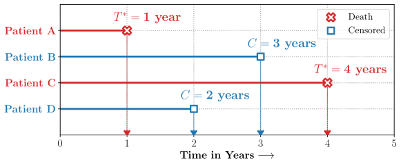
Figure 2: Censoring and Time-to-Event Predictions: Patients A and C died 1 and 4 years from entry into the study, whereas Patients B and D exited the study without experiencing death (were lost to follow up) at 2 and 3 years from entry in the study. Time-to-Event or Survival Regression thus involves estimates that are adjusted for individuals whose outcomes were censored.

For these individuals, we observe the censored survival time, $T$ and an indicator of if they were censored, $\Delta=T<C$. Assuming conditional independence between $T$ and $C$ ie. $T\perp C|X$ allows identification of the distribution of $\mathbb{P}(T|X)$.

For the censored individuals, we maximize the probability corresponding to the survival function. The likelihood, $\ell(\cdot)$ under censoring is thus given as

$$\bm{\ell}(\{{\bm{x}},{\bm{t}},\bm{\delta}\})\propto\mathbb{P}(T={\bm{t}}|X={\bm{x}})^{\delta}\mathbb{P}(T>{\bm{t}}|X={\bm{x}})^{1-\delta}.$$ (2)

Often in survival analysis literature likelihoods are expressed in terms of instantaneous hazard rates $\bm{\lambda}(t)$. The instantaneous hazard maybe defined as the event rate at a time $t$, conditional on survival $(T>t)$ till that time. Thus,

$$\bm{\lambda}(t)=\lim_{\textrm{d}t\rightarrow 0}\frac{\mathbb{P}(t\leq T<t+\textrm{d}t)}{\textrm{d}t\cdot S(t)}=\frac{\mathbb{P}(T=t)}{\bm{S}(t)}\quad\text{or, }\quad\bm{\lambda}(t)=-\frac{\textrm{d}}{\textrm{d}t}\log{\bm{S}}(t).$$ (3)

Now reasoning in terms of hazard rates, we can rewrite Equation 2 equivalently as

$$\bm{\ell}(\{{\bm{x}},{\bm{t}},\bm{\delta}\})\propto\bm{\lambda}({\bm{t}}|X={\bm{x}})^{\delta}{\bm{S}}({\bm{t}}|X={\bm{x}}).$$ (4)

Broadly the popular approaches for maximizing the likelihood above are classified as,

Parametric

Assumes the distribution of the time-to-event $\mathbb{P}(T|X={\bm{x}})$ is parametric like Weibull or Log-Normal. Examples includes the popular Accelerated Failure Time model.

Non-Parametric

Involves learning kernels or similarity functions of the input covariates followed by a non-parametric (Kaplan-Meier or Nelson-Aalen) estimation of the survival rate weighted with the learnt kernel.

Semi-Parametric

the Cox Proportional Hazards model and its extensions arguably, remain the most popular approaches and are classified as semi-parametric. The Cox model involves a two step estimation where the feature interactions are learnt through a parametric model followed by non-parametric estimation of the base survival (hazard) rate.

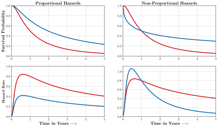
Figure 3: Non-Proportional Hazards: When the Proportional Hazards assumptions are satisfied, the Survival Curves and their corresponding Hazard Rates dominate each other and do not intersect. In many real world scenarios however, the survival curves. auton-survival includes flexible estimators of Time-to-Events in the presence of non-proportional hazards.

1.1 Fitting Survival Estimators

auton-survival includes the standard Cox Proportional Hazards (CPH) (Cox, 1972) to estimate time-to-event regression models. auton-survival allows the use of deep representation learning approaches to learn the Cox model as in Faraggi and Simon (1995); Katzman et al. (2018). Note that the standard Cox model is sensitive to the strong assumptions of Proportional Hazards which maybe mis-specified in real world scenarios (Figure 3). auton-survival thus includes deep latent variable survival regression models Deep Cox Mixtures (DCM) and Deep Survival Machines (DSM) (Nagpal et al., 2021b, c) that ease this restrictive assumption by modeling the conditional time-to-event distributions as mixtures of fixed size.

We demonstrate the use of auton-survival to predict long term mortality for 9,105 critically ill hospitalized patients from the SUPPORT (Study to Understand Prognoses Preferences Outcomes and Risks of Treatment) (Knaus et al., 1995; Connors et al., 1995) study; consisting of demographics, physiological measurements and outcomes followed up over a 5 year period.

⬇

1from auton_survival import datasets, preprocessing, models

2# Load the SUPPORT Dataset

3outcomes, features = datasets.load_dataset("SUPPORT")

4# Preprocess (Impute and Scale) the features

5features = preprocessing.Preprocessor().fit_transform(features)

6# Train a Deep Cox Proportional Hazards (DCPH) model

7model = models.cph.DeepCoxPH(layers=[100])

8model.fit(features, outcomes.time, outcomes.event)

9# Predict risk at specific time horizons.

10predictions = model.predict_risk(features, t=[8, 12, 16])

auton-survival also provides the convenient, SurvivalModel class that enables rapid experimentation via a consistent API by wrapping multiple regression estimators. In addition to the models above, SurvivalModel class also includes Random Survival Forests (RSF) (Ishwaran et al., 2008) a popular non-parametric survival model.

⬇

1from auton_survival import estimators A [Demo Notebook]

2# Train a Deep Survival Machines model using the SurvivalModel class.

3model = estimators.SurvivalModel(model=’dsm’)

4model.fit(features, outcomes)

5# Predict risk at time horizons.

6predictions = model.predict_risk(features, times=[8, 12, 16])

Additionally, the SurvivalRegressionCV class can be used to optimize survival regression models in a $K$-fold cross validation fashion over a user specified hyperparameter grid. Model selection is performed by selecting the model that minimizes the Integrated Brier Score.

⬇

1from auton_survival.experiments import SurvivalRegressionCV A [Demo Notebook]

2# Define the Hyperparameter grid to perform Cross Validation

3hyperparam_grid = {’n_estimators’ : [50, 100], ’max_depth’ : [3, 5],

4 ’max_features’ : [’sqrt’, ’log2’]}

5# Train a RSF model with cross-validation using the SurvivalRegressionCV class

6model = SurvivalRegressionCV(model=’rsf’, cv_folds=5, hyperparam_grid=hyperparam_grid)

7model.fit(features, outcomes)

1.2 Importance Weighting

Frequently in survival regression, we need to perform inference over a test dataset subject to distribution shift. Distribution shift can arise in multiple ways and affect the generalizability of a model. For simplicity, consider the covariate shift problem where, $\mathbb{P}_{\text{train}}(T,\Delta|X)=\mathbb{P}_{\text{test}}(T,\Delta|X)$ but $\mathbb{P}_{\text{train}}(X)\neq\mathbb{P}_{\text{test}}(X)$. auton-survival allows a flexible API to adjust for distribution shift involving Importance Weighted Empirical Risk Minimization (IWERM) (Sugiyama et al., 2007; Shimodaira, 2000) by weighted resampling of the training data with replacement at training time.

$$\mathop{\mathbb{E}}_{({\bm{x}},{\bm{t}},\bm{\delta})\sim\mathcal{D}_{\text{test}}}[\mathcal{L}({\bm{x}},{\bm{t}},\bm{\delta})] =\mathop{\mathbb{E}}_{({\bm{x}},{\bm{t}},\bm{\delta})\sim\mathcal{D}_{\text{test}}}\bigg{[}\ln\big{(}\bm{\lambda}(t|X={\bm{x}})^{\delta}\bm{S}(t|X={\bm{x}})\big{)}\bigg{]}$$ (5)

$$=\mathop{\int}_{{\bm{x}}\in\mathcal{X}}\mathop{\int}_{{\bm{t}}\in\mathcal{T}}\mathop{\int}_{\delta\in\{0,1\}}\ln\bigg{(}\bm{\lambda}(t|X={\bm{x}})^{\delta}\bm{S}(t|X={\bm{x}})\bigg{)}\mathbb{P}_{\text{test}}({\bm{x}},{\bm{t}},\delta)$$ (6)

$$=\mathop{\mathbb{E}}_{({\bm{x}},{\bm{t}},\bm{\delta})\sim\mathcal{D}_{\text{train}}}\big{[}\bm{w}({\bm{x}})\cdot\ln\big{(}\bm{\lambda}(t|X={\bm{x}})^{\delta}\bm{S}(t|X={\bm{x}})\big{)}\big{]},$$ (7)

$$\text{here, }\bm{w}(\bm{x}) \propto\frac{\mathbb{P}_{\text{test}}({\bm{x}})}{\mathbb{P}_{\text{train}}({\bm{x}})}\text{ are the estimated importance weights.}$$

⬇

1# Estimate Importance Weights with Logistic Regression

2from sklearn.linear_model import LogisticRegression

3p_target = LogisticRegression().fit(features, domains).predict_proba(features_source)

4imp_weights = p_target/(1-p_target) # Propensity Weighting

5# Train the Survival Regression Model

6from auton_survival.estimators import SurvivalEstimator

7model = SurvivalEstimator("dcph", layers=[100]) # Cox PH Model with 1 Hidden Layer

8model.fit(features=features_source, outcomes=outcomes_source, weights=imp_weights)

Cautionary Note (Censoring and Distribution Shift)

Label Shift

Covariate Shift

Figure 4: Prior probability and Covariate Shift in Time-to-Event (Survival) Regression. In situations where $A\rightarrow C$ the censoring rates, $C$ are dependent on the domain $A$, it may not be possible adjust for domain shift with standard importance weighting. Readers are thus advised to exercise caution in scenarios where shifts result in such complex interactions.

For the above covariate shift adjustment to work, the conditional distribution of the censoring times must be the same across the source and target domains. Additionally, is common to use importance weighting for adjustment in situations where $\mathbb{P}_{\textrm{train}}(T)\neq\mathbb{P}_{\textrm{test}}(T)$ This is commonly referred to as label shift or prior probability shift in Machine Learning (Figure 4). As in the case of covariate shift adjustment, this requires additional assumptions on the censoring distributions which might be violated in real-world situations. Readers are thus recommended to exercise appropriate caution when reasoning about whether importance weighting is an appropriate approach to adjust for distribution shift. A thorough discussion of the implications of this is beyond the current scope of this manuscript.

1.3 Counterfactual Survival Regression

Survival outcomes are often used to answer ‘what if?’ questions requiring inference of counterfactuals. We notate an intervention with an indicator ${\bm{a}}\in\{0,1\}$ and assume Strong Ignorability (Unconfoundedness) that the potential outcomes $T(1)$ and $T(0)$ are independent of the treatment assignment, ($A={\bm{a}}$) conditioned on the set of confounders ($X={\bm{x}}$) (Rubin, 2005). The estimated time-to-event outcome under intervention ($A={\bm{a}}$) is

$$\widehat{{\bm{S}}}\big{(}t|\text{do}(A={\bm{a}})\big{)}=\mathop{\mathbb{E}}_{{\bm{x}}\sim\mathcal{D}}\big{[}\widehat{\mathbb{E}}[\mathbf{1}\{T>t\}|X={\bm{x}},A={\bm{a}}]\big{]}.$$ (8)

Note that $\widehat{\mathbb{E}}[\mathbf{1}\{T>t\}|X={\bm{x}},A={\bm{a}}]$ is just a conditional estimator of survival learnt on the population under intervention ${\bm{a}}$. In practice thus, the counterfactual survival regression involves fitting separate regression models on the treated and control populations. auton-survival allows learning counterfactual models with $K$-fold cross-validation using the CounterfactualSurvivalCV class.

⬇

1from auton_survival.experiments import CounterFactualSurvivalRegressionCV

2grid = {’layers’ : [[], [100]], ’learning_rate’ : [1e-3, 1e-4]} # Hyperparameter Grid

3# Train a counterfactual Cox model with cross-validation.

4model = CounterfactualSurvivalRegressionCV(’dcph’, 5, hyperparam_grid=grid)

5model.fit(features, outcomes)

1.4 Time-Varying Survival Regression

Additionally auton-survival also includes time-varying implementations of Deep Survival Machines (Nagpal et al., 2021a) and Deep Cox Proportional Hazards model (Lee et al., 2021) thats involves the use of RNNs, LSTMs or GRUs (Chung et al., 2014; Hochreiter and Schmidhuber, 1997). Figure 5 presents time varying survival regression in auton-survival. For an individual with

Figure 5: Time Varying Survival Regression

time-to-event $\mathcal{T}_{i}$, we observe covariates ${\bm{x}}^{j}_{i}$ at multiple time points $t^{j}_{i}$. At each time-step, $j$ we estimate the distribution of the remaining time-to-event $T_{i}-t^{j}_{i}$. The representations of the input covariates $\widetilde{{\bm{x}}}^{(j+1)}_{i}$ at time-step $(j+1)$ are functions of the covariates, ${{\bm{x}}}^{(j+1)}_{i}$ and the representation of the preceeding time-step $\widetilde{{\bm{x}}}^{j}_{i}$. auton-survival automatically handles appropriate padding and batching for sequences of different lengths providing a convenient external API for time-varying survival regression.

⬇

1features, times, events = datasets.load_dataset(’PBC’, sequential = True)

2model = DeepRecurrentSurvivalMachines(k = 3, hidden = [100], typ = ’RNN’, layers = 2)

3model.fit(features, times, events)

2 Phenotyping Survival Data

Unsupervised Phenotyper

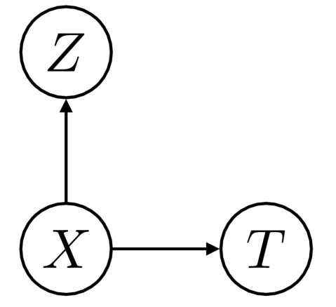
(a) Phenotype $Z$ is completely determined by the covariates $X$. The outcome is independent of the phenotype conditioned on the covariates. $(T\perp Z)|X$.

Supervised Phenotyper

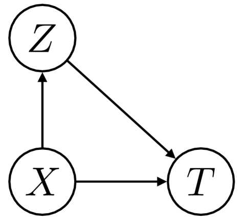
(b) The phenotype $Z$ effects the outcome, hence $T\not\perp Z|X$ . In this case, inference for $Z$ requires knowledge of the distribution of time-to-events $T$.

Counterfactual Phenotyper

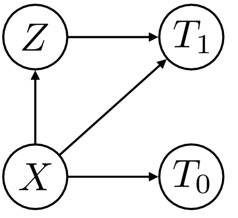
(c) The counterfactual phenotype effects the potential outcome under treatment, $T_{(1)}$, but is independent of the outcome under control, $T_{(0)}$.

Figure 6: DAG representations of the probabilitic phenotypers in auton-survival: $X$ represents the covariates, $T$ the time-to-event and $Z$ is the phenotype to be inferred.

Event incidence (survival) rates differ across groups of individuals with heterogeneous characteristics. Identifying groups of patients with similar survival rates can be used to derive insight about practices and interventions that can help improve longevity for such groups. While domain knowledge can help identify such subgroups, in practice there could be potentially complex, non-linear feature interactions that determine assignment to such groups, making identifiability difficult. In auton-survival, we refer to this group identification and survival assessment as phenotyping.

auton-survival offers multiple approaches to phenotyping that involve either the use of specific domain knowledge as in the case of the intersectional phenotyper, or a completely unsupervised approach that clusters based on the observed covariates. Additionally, auton-survival also offers phenotypers that explicitly involve supervision in the form of the observed outcomes and counterfactual to better inform the learnt phenotypes. Figure 6 demonstrates the probabilistic phenotypers offered by auton-survival as well as the corresponding assumption of conditional independence encoded in the models.

2.1 Intersectional Phenotyping

The IntersectionalPhenotyper class recovers groups, or phenotypes, of individuals over exhaustive combinations of user-specified categorical and numerical features. Numeric covariates are binned based on user-specified quantiles. The intersectional phenotyper is unsupervised, but does not have an explicit probabilistic interpretation. Figure 7 presents the intersectional phenogroups of cancer status and age group extracted on SUPPORT.

Figure 7: Intersectional Phenotypes.

⬇

1from auton_survival.phenotyping import IntersectionalPhenotyper A [Demo Notebook]

2# ’ca’ is cancer status. ’age’ is binned into two quantiles.

3phenotyper = IntersectionalPhenotyper(num_vars_quantiles=(0, .5, 1.0),

4 cat_vars=[’ca’], num_vars=[’age’])

5phenotypes = phenotyper.fit_phenotype(features)

6# Plot the phenogroup specific Kaplan-Meier survival estimate.

7auton_survival.reporting.plot_kaplanmeier(outcomes, phenotypes)

2.2 Unsupervised Phenotyping

Unsupervised phenotyping identifies groups based on structured similarity in the space of features. The ClusteringPhenotyper class achieves this by first performing dimensionality reduction of the input covariates ${\bm{x}}$, followed by clustering. The estimated probability of an individual to belong to a latent group $Z$ is computed as the distance to the cluster normalized by the sum of distance to other clusters. Thus,

$$\mathbb{P}(Z=k|X={\bm{x}})=\frac{\mathbf{d}({\bm{x}},\bar{{\bm{x}}}_{k})}{\mathop{\sum}_{j}\mathbf{d}({\bm{x}},\bar{{\bm{x}}}_{j})}.$$ (9)

Here $\mathbf{d}(\cdot)$ is the distance function corresponding to the underlying clustering method (for instance, ‘euclidean’ for $K$-means and ‘mahalonobis’ for a Gaussian Mixture Model.)

⬇

1from auton_survival.phenotyping import ClusteringPhenotyper A [Demo Notebook]

2# Dimensionality reduction using Principal Component Analysis (PCA) to 8 dimensions.

3dim_red_method, = ’pca’, 8

4# We use a Gaussian Mixture Model (GMM) with 3 components and diagonal covariance.

5clustering_method, n_clusters = ’gmm’, 3

6# Initialize the phenotyper with the above hyperparameters.

7phenotyper = ClusteringPhenotyper(clustering_method=clustering_method,

8 dim_red_method=dim_red_method,

9 n_components=n_components,

10 n_clusters=n_clusters)

11# Fit and infer the phenogroups.

12phenotypes = phenotyper.fit_phenotype(features)

13# Plot the phenogroup specific Kaplan-Meier survival estimate.

14auton_survival.reporting.plot_kaplanmeier(outcomes, phenotypes)

2.3 Supervised Phenotyping

Unsupervised Phenotyping

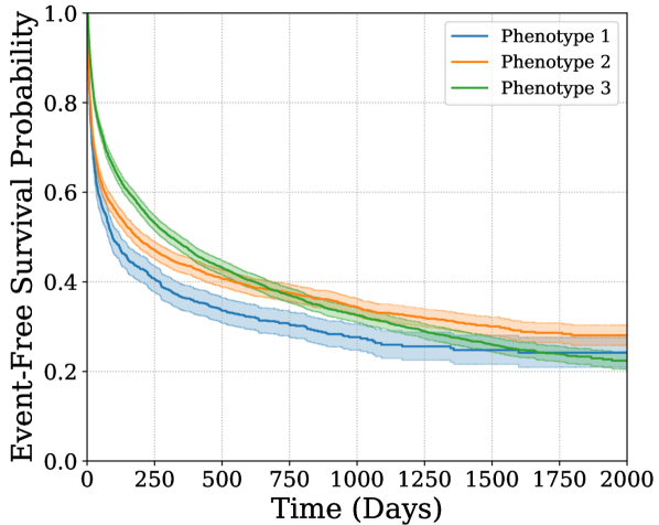
Supervised Phenotyping

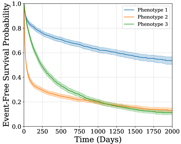
Phenotyping Purity Phenotyper Brier Score (BS) Integrated BS 1 year 2 years 5 years 5 years Unsupervised 0.246 $\pm$ 0.001 0.230 $\pm$ 0.004 0.187 $\pm$ 0.015 0.218 $\pm$ 0.004 Supervised 0.234 $\pm$ 0.002 0.219 $\pm$ 0.004 0.177 $\pm$ 0.014 0.207 $\pm$ 0.004

Figure 8: Supervised phenotyping with auton-survival extracts phenogroups in SUPPORT with higher discriminative power as indicated by the Kaplan-Meier curves and the lower Phenotyping Purity. The intersecting survival curves suggest the phenotypers’ ability to recover phenogroups that do not strictly adhere to assumptions of Proportional Hazards.

Supervised phenotyping seeks to explicitly identify latent groups of individuals with similar survival outcomes. Unlike unsupervised clustering, inferring supervised phenotypes requires time-to-events and the corresponding censoring indicators along with the covariates.

auton-survival provides utilities to perform supervised phenotyping as a direct consequence of training the Deep Survival Machines and Deep Cox Mixtures latent variable survival regression estimators. The inferred phenotypes can be obtained after learning these models using the predict_latent_z method. Note that these methods differ in the semantic meaning of the phenotypes they recover. DSM recovers phenotypes with similar parametric characteristics while DCM recovers phenotypes that adhere to proportional hazards.

⬇

1from auton_survival.models.dcm import DeepCoxMixtures A [Demo Notebook]

2# Instantiate a DCM Model with 3 phenogroups and a single hidden layer with size 100.

3model = DeepCoxMixtures(k = 3, layers = [100])

4model.fit(features, outcomes.time, outcomes.event, iters = 100, learning_rate = 1e-4)

5# Infer the latent Phenotpyes

6latent_z_prob = model.predict_latent_z(features)

7# Plot the phenogroup specific Kaplan-Meier survival estimate.

8auton_survival.reporting.plot_kaplanmeier(outcomes, latent_z_prob.argmax(axis=1))

Quantitative Evaluation of Phenotyping

We measure a phenotyper’s ability to extract subgroups, or phenogroups, with differential survival rates by fitting a Kaplan-Meier estimator within each phenogroup followed by estimating the (Integrated) Brier Score within each phenogroup. We refer to this as the phenotyping purity. Figure 8 demonstrates the use of phenotyping purity to compare discriminative power between unsupervised and supervised phenotyping.

⬇

1from auton_survival.metrics import phenotype_purity A [Demo Notebook]

2# Measure phenotype purity at event horizons of 1, 2 and 5 years.

3phenotype_purity(phenotypes, outcomes, strategy=’instantaneous’, time=[365,730,1825])

4# Measure phenotype purity at an event horizon of 5 years.

5phenotype_purity(phenotypes, outcomes, strategy=’integrated’, time=1825)

2.4 Counterfactual Phenotyping

In real world clinical scenarios, individuals demonstrate heterogeneous treatment effects to an intervention. Thus, clinical decision support often requires reasoning about which groups of individuals benefit least (or most) from a certain intervention. Such identification is often referred to as subgroup discovery or subgroup analysis. While there has been extensive study in subgroup recovery with binary or continuous outcomes (Dusseldorp and Van Mechelen, 2014; Lipkovich et al., 2011; Foster et al., 2011; Nagpal et al., 2020; Wang and Rudin, 2022), censored time-to-event outcomes are less studied in the context of phenotyping.

More formally we can describe counterfactual phenotyping as estimating a function $f({\bm{x}}):\mathbb{R}^{d}\to\{0,1\}$

$$f=\mathop{\textrm{arg min}}_{f\in\mathcal{F}}\mathbb{CATE}(\mathcal{D}|f(X)=1)\quad\textrm{such that}\quad\mathbb{E}[f(X)]>\alpha.$$ (10)

The first term here refers to the (Conditional) Average Treatment Effect within the discovered phenotype, while the second term controls the size of the phenotype.

Virtual Twins Survival Regression: auton-survival includes a Virtual Twins model (Foster et al., 2011) involving first estimating the potential outcomes under treatment and control using a counterfactual Deep Cox Proportional Hazards model, followed by regressing the difference in the estimated counterfactual Restricted Mean Survival Times using a Random Forest regressor.

⬇

1from auton_survival.phenotyping import SurvivalVirtualTwins

2# Instantiate the Survival Virtual Twins

3model = SurvivalVirtualTwins(horizon=365)

4model.fit(features, outcomes.time, outcomes.event, interventions)

5# Infer the estimated counterfactual phenotype probability.

6phi_probs = model.predict_latent_phi(features)

Cox Mixture Latent Variable Model: auton-survival also includes an implementation of the Cox Mixtures with Heterogenous Effects (CMHE) (Nagpal et al., 2022) model for counterfactual phenotyping. The CMHE model involves modelling the individual hazard rate under an intervention $(A={\bm{a}})$ as

$$\underbrace{\bm{\lambda}(t|X={\bm{x}},{\color[rgb]{0,0,0}Z=k},{\color[rgb]{0,0,0}\bm{\phi}=m},A=\bm{a})}_{\textrm{Conditional Hazard Rate}}=\overbrace{\bm{\lambda}_{k}(t)}^{\mathclap{\text{\shortstack{Base Survival Rate}}}}{\color[rgb]{0,0,0}\underbrace{\exp\big{(}h^{k}_{\bm{\theta}}({\bm{x}})\big{)}}_{\mathclap{\text{\shortstack{Effect of Confounders}}}}}{\color[rgb]{0,0,0}\overbrace{\exp(\omega_{m})^{\color[rgb]{0,0,0}\bm{a}}}^{\mathclap{\text{\shortstack{Treatment Effect}}}}},$$ (11)

where $(Z=k)$ is the base survival rate, $(\bm{\phi}=m)$ is the latent subgroup memberships that mediates the treatment effect.

⬇

1from auton_survival.models import cmhe A [Demo Notebook]

2# Instantiate the Cox Mixture with Heterogenous Effects model

3model = cmhe.DeepCoxMixturesHeterogenousEffects(k=1, g=2, layers=[100])

4model.fit(features, outcomes.time, outcomes.event, interventions,

5 iters=iters, learning_rate=learning_rate, batch_size=batch_size)

6# Infer the estimated counterfactual phenotypes.

7latent_phi_probs = model.predict_latent_phi(features)

3 Evaluation

3.1 Censoring-Adjusted Evaluation Metrics

The survival model performance can be evaluated using the following metrics, among others. auton-survival offers utilities to compute these metrics along with bootstrapped confidence intervals with a convenient API.

Brier Score (BS): The Brier Score involves computing the Mean Squared Error of the estimated survival probabilities, $\widehat{\mathbb{P}}(T>t|X={\bm{x}})=f({\bm{x}},t)$ at a specified time horizon, $t$. As a proper scoring rule, Brier Score gives a sense of both discrimination and calibration.

Under the assumption that the censoring distribution is independent of the time-to-event, we can obtain an unbiased, censoring adjusted estimate of the Brier Score $\widehat{\text{BS}}_{\text{IPCW}}(t)$ using inverse probability of censoring weights (IPCW) from a Kaplan-Meier estimator of the censoring distribution, $\hat{G}(.)$ as proposed in Graf et al. (1999); Gerds and Schumacher (2006).

$$\text{BS}(t) =\mathbb{E}_{\mathcal{D}}\big{[}\big{(}\bm{1}\{T_{i}>t\}-\widehat{\mathbb{P}}(T>t|X={\bm{x}})\big{)}^{2}\big{]}$$

$$\widehat{\text{BS}}_{\text{IPCW}}(t) =\frac{1}{n}\sum_{i=1}^{n}\bigg{[}\frac{f({\bm{x}}_{i},t)^{2}\bm{1}\{T\leq t,\delta_{i}=1\}}{\hat{G}_{i}(T_{i})}+\frac{\big{(}1-f({\bm{x}}_{i},t))^{2}\bm{1}\{T>t\}}{\hat{G}_{i}(t)}\bigg{]}.$$

Area under ROC Curve (AUC): ROC Curves are extensively used in classification tasks where the true positive rate (TPR) is plotted against the false positive rate (1-true negative rate, or TNR) to measure the in model discriminative power over all output thresholds.

To enable the use of ROC curves to assess the performance of survival models subject to censoring, we employ the technique proposed by Uno et al. (2007); Hung and Chiang (2010), which treats the TPR as time-dependent on a specified horizon, $t$ and adjusts survival probabilities, $f({\bm{x}},t)$, using the IPCW from a Kaplan-Meier estimator of the censoring distribution, $\hat{G}(t)$. Estimating the TNR requires observing outcomes for each individual, only uncensored instances are used. Refer to Kamarudin et al. (2017) for details on computing ROC curves in the presence of censoring.

$$\widehat{\text{TPR}}(c,t)=\frac{\sum\limits_{i=1}^{n}\frac{\delta_{i}}{\hat{G}(T_{i})}\cdot\bm{1}\{f({\bm{x}}_{i},t)>c,T_{i}\leq t\}}{\sum\limits_{i=1}^{n}\frac{\delta_{i}}{\hat{G}(T_{i})}\cdot\bm{1}\{T_{i}<t\}\cdot};\quad\widehat{\text{TNR}}(c,t)=\frac{\sum\limits_{i=1}^{n}\bm{1}\{f({\bm{x}}_{i},t)\leq c,T_{i}>t\}}{\sum\limits_{i=1}^{n}\bm{1}\{T_{i}>t\}}$$

Time Dependent Concordance Index ($C^{\text{td}}$): Concordance Index compares risks across all pairs of individuals within a fixed time horizon, $t$, to estimate ability to appropriately rank instances relative to each other in terms of their risks, $f({\bm{x}},t)$.

$$C^{td}(t)=\mathbb{P}\big{(}f({\bm{x}}_{i},t)\leq f({\bm{x}}_{j},t)|\delta_{i}=1,T_{i}<T_{j},T_{i}\leq t\big{)}$$

We employ the censoring adjusted estimator for $C^{\text{td}}$ that exploits IPCW estimates from a Kaplan-Meier estimate of the censoring distribution. Further details can be found in Uno et al. (2011) and Gerds et al. (2013).

⬇

1from auton_survival.metrics import survival_regression_metric

2# Infer event-free survival probability from model

3predictions = model.predict_survival(features, times)

4# Compute Brier Score, Integrated Brier Score

5# Area Under ROC Curve and Time Dependent Concordance Index

6metrics = [’brs’, ’ibs’, ’auc’, ’ctd’]

7for metric in metrics

8 score = survival_regression_metric(metric, outcomes_train, outcomes_test, predictions_test, times=times)

3.2 Comparing Treatment Arms

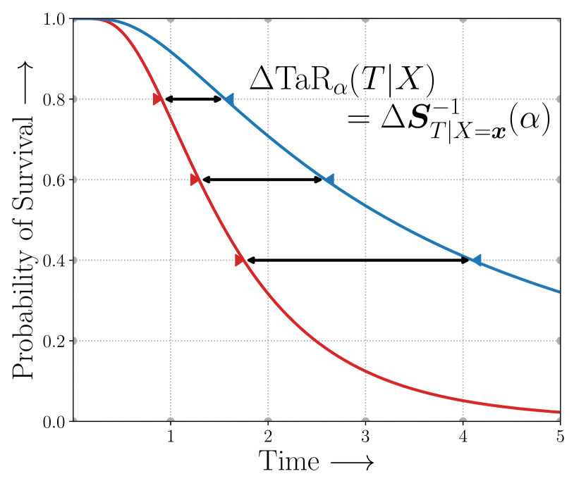
(a) Time at Risk (TaR)

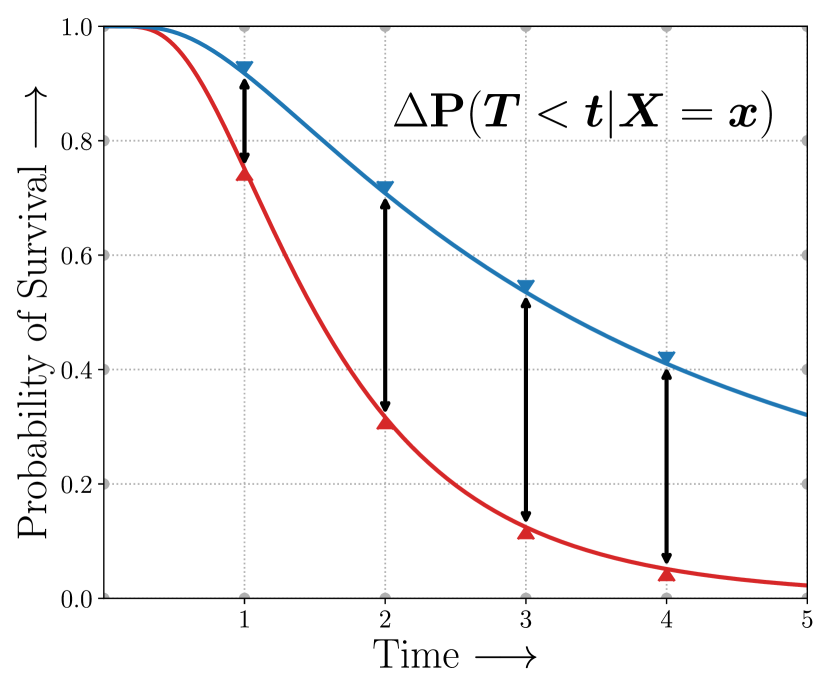
(b) Risk at Time

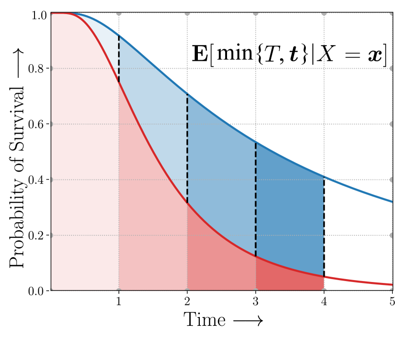
(c) RMST

Figure 9: Treatment effects measured in terms of the difference in metrics computed for treatment and control groups including (a) the time at a specified level of risk (b) risk at a certain time and (c) the expected survival time over a truncated time horizon.

Hazard Ratio

Assuming the proportional hazards assumptions holds, the treatment effect can be modelled as the ratio of hazard rates between the treatment and control arms. This corresponds to fitting a univariate Cox Proportional Hazards model and is arguably the most popular approach in estimating treatment effects for censored time-to-events.

Time at Risk (TaR)

Time at Risk (TaR) (Figure 9) measures time-to-event at a specified level of risk. Computing TaR may be of interest when maximum permissible outcome risk is predefined and the corresponding time-to-event is the deciding factor for assessing treatment benefit at that risk level.

$$\operatorname{TaR}_{\alpha}(T|X)=\sup_{t}\big{\{}t\in\mathbb{R}^{+}:\bm{S}_{T|X}(t)<\alpha\big{\}}=\bm{S}^{-1}_{T|X}(\alpha)$$ (12)

Risk at Time

Risk at Time (Figure 9) measures risk at a specified time horizon. This metric may be of interest when treating survival as a binary outcome over a specific time horizon.

$$\textrm{Risk-at-Time}(t|X={\bm{x}})=\mathbb{P}(T<t|X={\bm{x}})=1-{\bm{S}}(t|X={\bm{x}})$$ (13)

Restricted Mean Survival Time (RMST)

The RMST (Figure 9) is the expected (or mean) time-to-event conditioned on a specified time horizon. Mathematically, the RMST is $\mathbb{E}[\mathrm{min}\{T,{\bm{t}}\}|X={\bm{x}}]$ and translates into the area under the survival curve till time ${\bm{t}}$.

$$\mathrm{RMST}_{{\bm{t}}}(T|X={\bm{x}}) =\mathbb{E}[\mathrm{min}\{T,{\bm{t}}\}|X={\bm{x}}]$$ (14)

$$=\int_{0}^{t}{\bm{S}}(\bm{t}|X={\bm{x}})\textrm{d}\bm{t}.$$

RMST might be preferred over Hazard Ratio in comparing treatment arms where there is reason to believe that the proportional hazards assumption is violated.

⬇

1from auton_survival.metrics import treatment_effect

2# Compute the difference in RMST between treatment and control groups

3effect = treatment_effect(metric=’restricted_mean’, outcomes=outcomes

4 treatment_indicator=treatment_indicator,

5 weights=None, horizon=120, n_bootstrap=500)

3.3 Propensity Adjusted Treatment Effects

Differences in the values of metrics specified in Section 3.2 across treatment arms is often averaged over the population to estimate net benefit or the average treatment $(\mathbb{ATE})$,

$$\mathbb{ATE}(\mathcal{D},f)=\mathop{\mathbb{E}}_{{\bm{x}}\sim\mathcal{D}}\big{[}\mathbb{E}[f_{1}(x)-f_{0}(x)|X={\bm{x}}]\big{]}$$

Directly computing the metrics in above in an observational settings would result in mis-estimations of treatment effects as it would not adjust for potential confounders that influence both treatment assignment and the outcome. auton-survival supports the computation of propensity-adjusted treatment effects in terms of the above metrics through bootstrap resampling the dataset, $\mathcal{D}$ with replacement. Here the resampling weights are obtained using inverse propensity of treatment weighting (IPTW). The bootstrapped treatment effect thus converges to the Thompson-Horvitz estimate of the Treatment Effect.

$$\mathbb{ATE}(\mathcal{D}^{*},f)=\mathop{\mathbb{E}}_{{\bm{x}}\sim\mathcal{D}^{*}}\big{[}\mathbb{E}[f_{1}(x)-f_{0}(x)|X={\bm{x}}]\big{]};\quad\mathcal{D}^{*}\sim\frac{1}{\widehat{\mathbb{P}}(A|X)}\cdot\mathbb{P}^{*}(\mathcal{D})$$ (15)

The auton-survival function treatment_effect function supports sample weight inputs in the form of treatment propensity scores, such as obtained from scaled classification model scores that estimate probability of treatment.

⬇

1from auton_survival.metrics import treatment_effect

2from sklearn.linear_model import LogisticRegression

3# Train a classification model to compute "treatment" propensity scores

4model = LogisticRegression(penalty=’l2’).fit(features, treatment_indicator)

5treatment_propensity = model.predict_proba(features)[:, 1]

6# Compute the treatment effect after adjusting for treatment propensity

7adjusted_effect = treatment_effect(metric=’hazard_ratio’, outcomes=outcomes

8 treatment_indicator=treatment_indicator,

9 weights=treatment_propensity, n_bootstrap=500)

4 Case Study: Regional disparities in Breast Cancer Incidence

Sample Size and RMST by Region Region Size RMST Greater California 47,757 108.9 $\pm$ 0.261 New Jersey 27,665 107.3 $\pm$ 0.352 Greater Georgia 14,212 106.8 $\pm$ 0.559 Louisiana 11,837 104.1 $\pm$ 0.598 Kentucky 11,581 106.4 $\pm$ 0.610 All Regions 113,052 107.5 $\pm$ 0.189

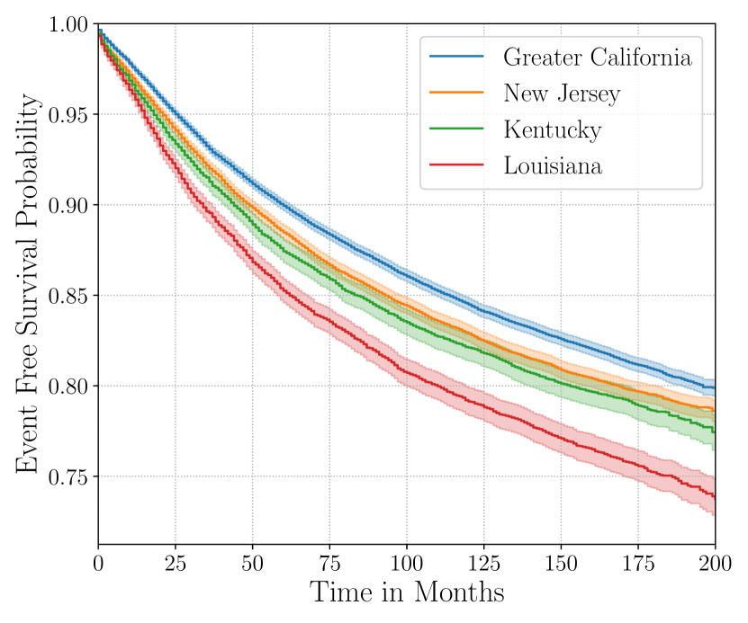
Figure 10: Breast cancer survival from the cohort subset of the SEER study. Notice discrepancies in the Kaplan-Meier estimated survival rates when stratified by the geographic region. Similarly, regional discrepancies in expected time-to-event are highlighed by mean (95% CI) RMST computed for bootstrap samples conditioned on a 10-year horizon.

The SEER registry established by the National Cancer Institute consists of patient demographic and tumour morphology data and long term incidence information of approximately one-third of the U.S. population (Ries et al., 2008). This study is a retrospective analysis of the SEER data. For this study, we consider a subset of 113,052 patients from Greater California, Kentucky, Louisiana, New Jersey and Georgia diagnosed with breast cancer between a four year period from January 2000 to December 2003. We consider all-cause mortality as the outcome of interest with a maximum follow up period of 18 years from January, 2000. Along with outcomes we also consider additional variables including age, race, tumour morphology and treatments administered. A complete list of the variables considered in this study can be found in Appendix B.

4.1 The Effect of Geographical Region on Breast Cancer Mortality

It is evident that there are discrepancies between the observed mortality rates stratified by the geographic region (Figure 10). A natural question arises as to whether this discrepancy can be attributed to geographic region or other socio-economic or physiological confounding factors that effect both belonging to these regions and the outcome.

We attempt to provide insight into this question by assessing the effect size via the Potential Outcomes framework by considering the region as an intervention. We first estimate the counterfactual survival rates across treatment arms to evaluate the effect of treatment on event-free survival rates. We further verify our findings by comparing treatment effects before and after adjusting for treatment propensity by inverse propensity weighting.

Counterfactual Survival Estimation

To adjust estimates of survival with counterfactual estimation, we train two separate Deep Cox models as described in Section 1.3 on data from Greater California and Louisiana as counterfactual regressors. The fitted regressors are then applied to estimate the survival curves for each instance, which are then averaged over treatment groups to compute the domain-specific survival rate.

Figure 11 presents the counterfactual survival rates compared with the survival rates obtained from a Kaplan-Meier estimator. The Kaplan-Meier estimator does not adjust for confounding and so overestimates treatment effect as evidenced from the extent that survival rates differ between regions. Counterfactual regression adjusts for confounding factors and predicts more similar survival rates between regions.

Figure 11: The Kaplan-Meier estimator overestimates effect of region on mortality compared with the counterfactual regression model, which reduces discrepancy in survival rates between regions.

Propensity Adjusted Treatment Effects

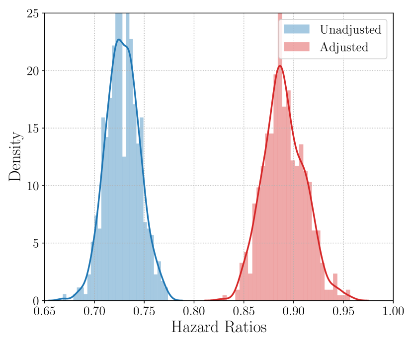
(a) Hazard Ratios

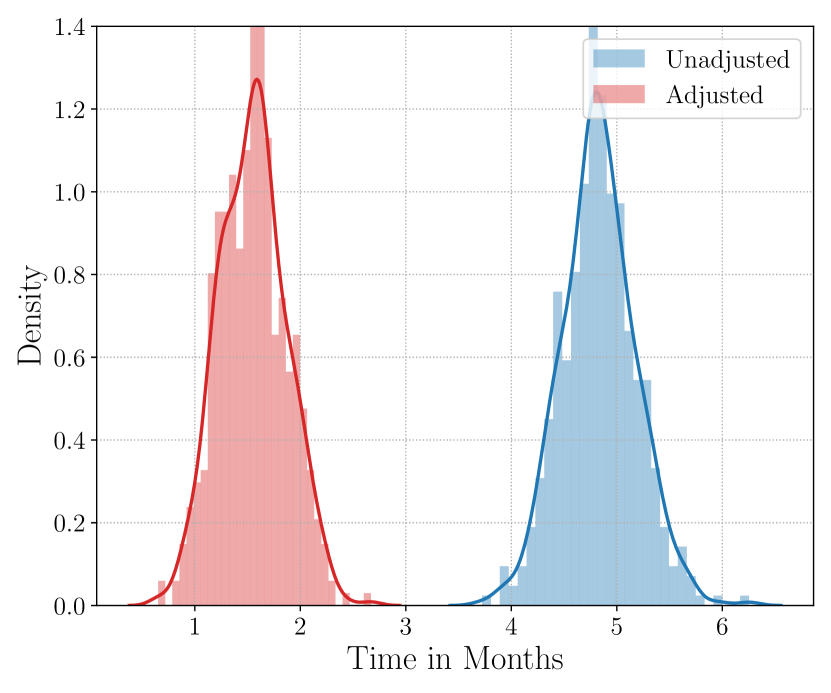
(b) RMST

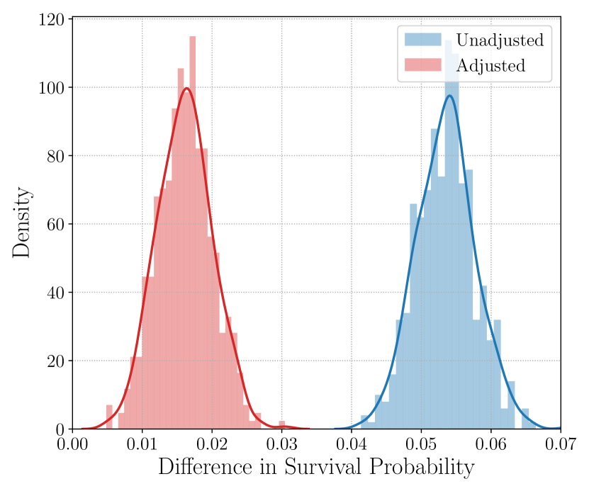
(c) Risk Difference

Treatment Effect	10-year Event Horizon
	Hazard Ratio	RMST	Risk Difference
Unadjusted	0.728 $\pm$ 0.032	4.829 $\pm$ 0.684	0.054 $\pm$ 0.008
Adjusted	0.890 $\pm$ 0.040	1.549 $\pm$ 0.618	0.016 $\pm$ 0.008

Figure 12: Estimated probability densities of the bootstrapped treatment effects to assess discrepancies in survival across regions. When bootstrapping is performed with weighted sampling based on region propensity to adjust for confounders, the discrepancies in survival between Greater California and Louisiana are much less pronounced. Bootstrap mean (standard deviation) results shown in the table summarize the observed mitigated difference.

A alternative method to assess effect size of the geographical region on survival involves comparing differences after adjusting for treatment propensity. We trained a Logistic Regression with an $\ell_{2}$ penalty by regression the Geographical Region on the set of confounding variables. The propensity scores were then employed as sampling weights for the treatment effects in terms of hazard ratios, restricted mean survival time (RMST), and risk difference as in Figure 12. Adjusting for region propensity noticeably mitigates differences in treatment effects, indicating that mortality due to breast cancer is likely explained by confounding socio-economic and physiological factors rather than solely geographic region.

⬇

1from auton_survival.metrics import treatment_effect

2from sklearn.linear_model import LogisticRegression

3# Create "treatment" labels

4domain = regions==’Louisiana’

5# Train a logistic regression model to compute "domain" propensity scores

6model = LogisticRegression(penalty=’l2’).fit(features, domain)

7propensity = model.predict_proba(features)[:, 1]

8# Compute the treatment effect before and after adjusting for treatment propensity

9effect = treatment_effect(metric=’hazard_ratio’, outcomes, domain,

10 n_bootstrap=500)

11adjusted_effect = treatment_effect(metric=’hazard_ratio’, outcomes, domain, weights=propensity, n_bootstrap=500)

4.2 Domain Adaptation

Area under ROC Curve

Louisiana $\rightarrow$ Greater California

Horizon	1-Year	2-Year	5-Year
Unadjusted	0.8398	0.8177	0.8010
Adjusted	0.8449	0.8220	0.8063

Greater California $\rightarrow$ Louisiana

Horizon	1-Year	2-Year	5-Year
Unadjusted	0.8598	0.8343	0.8163
Adjusted	0.8603	0.8348	0.8182

Brier Score

Louisiana $\rightarrow$ Greater California

Horizon	1-Year	2-Year	5-Year
Unadjusted	0.0675	0.0967	0.1154
Adjusted	0.0673	0.0963	0.1148

Greater California $\rightarrow$ Louisiana

Horizon	1-Year	2-Year	5-Year
Unadjusted	0.0858	0.1119	0.1312
Adjusted	0.0856	0.1118	0.1307

Table 1: Domain Adaptation with importance weighting improves both calibration and discriminative performance when applying models trained on one domain to the other.

Consider a scenario when training data is available from Greater California (Lousiana) and is to be used to train models to estimate risk for patients in Lousiana (Greater California). Discrepancies in the data distributions would naturally also translate into poorer generalization when using these models for individual level survival regression.

It would thus help adjusting for these distributional differences using IWERM as introduced Section 1.2. We train a logistic regression with an $\ell_{2}$ penalty to estimate the probability of an individual belonging to one of the two regions. The estimated probabilities are then used as importance weights to resample th individuals when training a Cox Model.

Table 1 present the performance of a linear Cox model in terms of discriminative performance (Area under ROC curve) and well as calibration (Brier Score) at predicting all cause mortality within 5, 10 and 15 years of entry into the study. Notice that the importance weighted Cox model has better discriminative performance and calibration as compared to the the unadjusted model.

⬇

1from auton_survival.estimators import SurvivalModel

2from sklearn.linear_model import SGDClassifier

3regions=[’Greater California’, ’Louisiana’]

4for source in regions:

5 for target in regions:

6 # Train a Logistic Regression to estimate treatment propensity scores

7 domain_model = SGDClassifier(loss=’log’, penalty=’l2’, alpha=.1)

8 domain_model.fit(features, regions==target)

9 probs = domain_model.predict_proba(features[regions==source])[:, 1]

10 # Use propensity scores to compute sample weights

11 weights = ((probs)/(1-probs))**0.2

12 # Fit DCPH model with weighted resampling

13 model = SurvivalModel(model=’dcph’, layers=[100])

14 model.fit(features[regions==source], outcomes[regions==source],

15 weights, resample_size=10.0)

Conclusion

We presented auton-survival, an open source Python package encapsulating multiple pipelines to analyze censored time-to-event data ubiquitous in healthcare. Through the use of multiple code examples, notebooks, and illustrations we demonstrate the efficacy of auton-survival to analyze complex healthcare data and answer clinical and epidemiological questions including real-world case studies.

We acknowledge auton-survival as one step towards promoting reproducible machine learning research for healthcare. We believe that the broader use of software packages such as ours will help accelerate and systematize impactful machine learning research for healthcare. We expect that ongoing and future collaborations with the machine learning and healthcare communities will allow us to further enhance the collection of open-source survival regression methodologies that can support reproducible analysis of censored time-to-event data.

Appendix A Comparison to Other Packages

In the code snippets below we will compare the API of auton-survival with the popular alternative, pycox to train a Deep Cox PH model on the SUPPORT dataset.

⬇

1from auton_survival import datasets, preprocessing

2# Load the SUPPORT Dataset

3outcomes, features = datasets.load_dataset("SUPPORT")

4# Preprocess (Impute and Scale) the features

5features = preprocessing.Preprocessor().fit_transform(features)

Training a Deep Cox Proportional Hazards model with pycox

⬇

1from torchtuples.tt.practical import MLPVanilla

2from pycox.models import CoxPH

3net = MLPVanilla(features.shape[1], [100], 1, output_bias=False) # Instantiate an MLP

4model = CoxPH(net, tt.optim.Adam) # Instantiate a pycox model.

5# Fit the pycox model.

6model.fit(features, (outcomes.time, outcomes.event), batch_size=256, epochs=10)

Training a Deep Cox Proportional Hazards model with $\href https://www.cs.cmu.edu/\leavevmode\nobreak\ chiragn/redirects/auton_survival/main.html{}$.

⬇

1from auton_survival import models

2# Train a Deep Cox Proportional Hazards (DCPH) model

3model = models.cph.DeepCoxPH(layers=[100])

4model.fit(features, outcomes.time, outcomes.event, batch_size=256,)

5# Predict risk at specific time horizons.

6predictions = model.predict_risk(features, t=[8, 12, 16])

Utility / Package	lifelines	pycox	scikit-survival	auton-survival
Deep Survival Models	✗	✓	✗	✓
Time-Varying Survival Analysis	✓	✗	✗	✓
Counterfactual Estimation	✗	✗	✗	✓
Subgroup Identification (Phenotyping)	✗	✗	✗	✓
Treatment Effect Estimation	✓	✗	✗	$\bigcirc$
Regression Metrics	✓	✓	✓	$\bigcirc$
Cross-Validation	✗	✗	✗	✓
Preprocessing	✗	✓	✓	✓
Documentation and Examples	✓	✓	✓	✓

Table 2: A comparison of auton-survival to other open-source python packages for survival analysis. $\bigcirc$ indicates that the utility depends on one of other survival analysis packages.

Appendix B Additional details on the SEER case study

Name	Description
AGE	Age of participant
SEX	Sex of participant
RACE1V	Race/Ethnicity of participant
PRIMSITE	Site in which the primary tumor originated.
LATERAL	Side of a paired organ or body on which the tumor originated.
HISTO3V	Histologic Type ICD-O-3.
BEHO3V	Behavior Code ICD-O-3.
DX_CONF	Diagnostic Confirmation.
SURGPRIF	Surgery of Primary Site.
SURGSITF	The surgical removal of distant tissue beyond the primary site.
NUMNODES	Number of Examined Nodes
NO_SURG	Reason for no surgery.
SURGSITE	The removal of distant tissue beyond the primary site.
EOD10_SZ	Tumor size.
EOD10_EX	Tumor extension.
EOD10_ND	The highest specific lymph node chain that is involved by the tumor.
EOD10_PN	Regional nodes positive.
EOD10_NE	regional nodes examined.
MALIGCOUNT	Total number of In Situ/malignant tumors for patient.
BENBORDCOUNT	Total number of benign/borderline tumors.

Table 3: List of confounding features used for experiments involving the the SEER dataset.

References

- Chapfuwa et al. (2018) Paidamoyo Chapfuwa, Chenyang Tao, Chunyuan Li, Courtney Page, Benjamin Goldstein, Lawrence Carin Duke, and Ricardo Henao. Adversarial time-to-event modeling. In International Conference on Machine Learning, pages 735–744. PMLR, 2018.
- Chung et al. (2014) Junyoung Chung, Caglar Gulcehre, KyungHyun Cho, and Yoshua Bengio. Empirical evaluation of gated recurrent neural networks on sequence modeling. arXiv preprint arXiv:1412.3555, 2014.
- Connors et al. (1995) Alfred F Connors, Neal V Dawson, Norman A Desbiens, William J Fulkerson, Lee Goldman, William A Knaus, Joanne Lynn, Robert K Oye, Marilyn Bergner, Anne Damiano, et al. A controlled trial to improve care for seriously iii hospitalized patients: The study to understand prognoses and preferences for outcomes and risks of treatments (support). Jama, 274(20):1591–1598, 1995.
- Cox (1972) D. R. Cox. Regression models and life-tables. Journal of the Royal Statistical Society. Series B (Methodological), 34(2):187–220, 1972.
- Davidson-Pilon (2019) Cameron Davidson-Pilon. lifelines: survival analysis in python. Journal of Open Source Software, 4(40):1317, 2019.
- Dusseldorp and Van Mechelen (2014) Elise Dusseldorp and Iven Van Mechelen. Qualitative interaction trees: a tool to identify qualitative treatment–subgroup interactions. Statistics in medicine, 33(2):219–237, 2014.
- Faraggi and Simon (1995) David Faraggi and Richard Simon. A neural network model for survival data. Statistics in medicine, 14(1):73–82, 1995.
- Foster et al. (2011) Jared C Foster, Jeremy MG Taylor, and Stephen J Ruberg. Subgroup identification from randomized clinical trial data. Statistics in medicine, 30(24):2867–2880, 2011.
- Gerds and Schumacher (2006) Thomas A Gerds and Martin Schumacher. Consistent estimation of the expected brier score in general survival models with right-censored event times. Biometrical Journal, 48(6):1029–1040, 2006.
- Gerds et al. (2013) Thomas A Gerds, Michael W Kattan, Martin Schumacher, and Changhong Yu. Estimating a time-dependent concordance index for survival prediction models with covariate dependent censoring. Statistics in Medicine, 32(13):2173–2184, 2013.
- Graf et al. (1999) Erika Graf, Claudia Schmoor, Willi Sauerbrei, and Martin Schumacher. Assessment and comparison of prognostic classification schemes for survival data. Statistics in medicine, 18(17-18):2529–2545, 1999.
- Hochreiter and Schmidhuber (1997) Sepp Hochreiter and Jürgen Schmidhuber. Long short-term memory. Neural computation, 9(8):1735–1780, 1997.
- Hung and Chiang (2010) Hung Hung and Chin-tsang Chiang. Optimal composite markers for time-dependent receiver operating characteristic curves with censored survival data. Scandinavian journal of statistics, 37(4):664–679, 2010.
- Ishwaran et al. (2008) H. Ishwaran, Udaya B. Kogalur, Eugene H. Blackstone, and Michael S. Lauer. Random survival forests. The Annals of Applied Statistics, 2(3), 2008.
- Kamarudin et al. (2017) Adina Najwa Kamarudin, Trevor Cox, and Ruwanthi Kolamunnage-Dona. Time-dependent roc curve analysis in medical research: current methods and applications. BMC medical research methodology, 17(1):53, 2017.
- Katzman et al. (2018) Jared L Katzman, Uri Shaham, Alexander Cloninger, Jonathan Bates, Tingting Jiang, and Yuval Kluger. Deepsurv: personalized treatment recommender system using a cox proportional hazards deep neural network. BMC medical research methodology, 18(1):1–12, 2018.
- Knaus et al. (1995) W. A. Knaus, Harrell F. E., Lynn J, and et al. The support prognostic model: Objective estimates of survival for seriously ill hospitalized adults. Annals of Internal Medicine, 122:191–203, 1995.
- Kvamme et al. (2019) Håvard Kvamme, Ørnulf Borgan, and Ida Scheel. Time-to-event prediction with neural networks and cox regression. arXiv preprint arXiv:1907.00825, 2019.
- Lee et al. (2018) Changhee Lee, William Zame, Jinsung Yoon, and Mihaela Van Der Schaar. Deephit: A deep learning approach to survival analysis with competing risks. In Proceedings of the AAAI conference on artificial intelligence, volume 32, 2018.
- Lee et al. (2021) Hyun Gi Lee, Evan Sholle, Ashley Beecy, Subhi Al’Aref, and Yifan Peng. Leveraging deep representations of radiology reports in survival analysis for predicting heart failure patient mortality. arXiv preprint arXiv:2105.01009, 2021.
- Lipkovich et al. (2011) Ilya Lipkovich, Alex Dmitrienko, Jonathan Denne, and Gregory Enas. Subgroup identification based on differential effect search—a recursive partitioning method for establishing response to treatment in patient subpopulations. Statistics in medicine, 30(21):2601–2621, 2011.
- Nagpal et al. (2020) Chirag Nagpal, Dennis Wei, Bhanukiran Vinzamuri, Monica Shekhar, Sara E Berger, Subhro Das, and Kush R Varshney. Interpretable subgroup discovery in treatment effect estimation with application to opioid prescribing guidelines. In Proceedings of the ACM Conference on Health, Inference, and Learning, pages 19–29, 2020.
- Nagpal et al. (2021a) Chirag Nagpal, Vincent Jeanselme, and Artur Dubrawski. Deep parametric time-to-event regression with time-varying covariates. In Survival Prediction-Algorithms, Challenges and Applications, pages 184–193. PMLR, 2021a.
- Nagpal et al. (2021b) Chirag Nagpal, Xinyu Li, and Artur Dubrawski. Deep survival machines: Fully parametric survival regression and representation learning for censored data with competing risks. IEEE Journal of Biomedical and Health Informatics, 25(8):3163–3175, 2021b.
- Nagpal et al. (2021c) Chirag Nagpal, Steve Yadlowsky, Negar Rostamzadeh, and Katherine Heller. Deep cox mixtures for survival regression. In Machine Learning for Healthcare Conference, pages 674–708. PMLR, 2021c.
- Nagpal et al. (2022) Chirag Nagpal, Mononito Goswami, Keith Dufendach, and Artur Dubrawski. Counterfactual phenotyping with censored time-to-events. arXiv preprint arXiv:2202.11089, 2022.
- Paszke et al. (2019) Adam Paszke, Sam Gross, Francisco Massa, Adam Lerer, James Bradbury, Gregory Chanan, Trevor Killeen, Zeming Lin, Natalia Gimelshein, Luca Antiga, et al. Pytorch: An imperative style, high-performance deep learning library. Advances in neural information processing systems, 32, 2019.
- Pedregosa et al. (2011) Fabian Pedregosa, Gaël Varoquaux, Alexandre Gramfort, Vincent Michel, Bertrand Thirion, Olivier Grisel, Mathieu Blondel, Peter Prettenhofer, Ron Weiss, Vincent Dubourg, et al. Scikit-learn: Machine learning in python. the Journal of machine Learning research, 12:2825–2830, 2011.
- Pölsterl (2020) Sebastian Pölsterl. scikit-survival: A library for time-to-event analysis built on top of scikit-learn. J. Mach. Learn. Res., 21(212):1–6, 2020.
- Ranganath et al. (2016) Rajesh Ranganath, Adler Perotte, Noémie Elhadad, and David Blei. Deep survival analysis. In Machine Learning for Healthcare Conference, pages 101–114. PMLR, 2016.
- Ries et al. (2008) LAG Ries, D Melbert, M Krapcho, DG Stinchcomb, N Howlader, MJ Horner, A Mariotto, BA Miller, EJ Feuer, SF Altekruse, et al. Seer cancer statistics review, 1975–2005. Bethesda, MD: National Cancer Institute, 2999, 2008.
- Rubin (2005) Donald B Rubin. Causal inference using potential outcomes: Design, modeling, decisions. Journal of the American Statistical Association, 100(469):322–331, 2005.
- Shimodaira (2000) Hidetoshi Shimodaira. Improving predictive inference under covariate shift by weighting the log-likelihood function. Journal of statistical planning and inference, 90(2):227–244, 2000.
- Sugiyama et al. (2007) Masashi Sugiyama, Matthias Krauledat, and Klaus-Robert Müller. Covariate shift adaptation by importance weighted cross validation. Journal of Machine Learning Research, 8(5), 2007.
- Uno et al. (2007) Hajime Uno, Tianxi Cai, Lu Tian, and Lee-Jen Wei. Evaluating prediction rules for t-year survivors with censored regression models. Journal of the American Statistical Association, 102(478):527–537, 2007.
- Uno et al. (2011) Hajime Uno, Tianxi Cai, Michael J Pencina, Ralph B D’Agostino, and LJ Wei. On the c-statistics for evaluating overall adequacy of risk prediction procedures with censored survival data. Statistics in medicine, 30(10):1105–1117, 2011.
- Wang and Rudin (2022) Tong Wang and Cynthia Rudin. Causal rule sets for identifying subgroups with enhanced treatment effects. INFORMS Journal on Computing, 2022.
- Yu et al. (2011) Chun-Nam Yu, Russell Greiner, Hsiu-Chin Lin, and Vickie Baracos. Learning patient-specific cancer survival distributions as a sequence of dependent regressors. Advances in neural information processing systems, 24, 2011.