Numerical evaluation of dual norms via the MM algorithm

Abstract

We deal with the problem of numerically computing the dual norm, which is important to study sparsity-inducing regularizations (Jenatton et al.,, 2011; Bach et al.,, 2012). The dual norms find application in optimization and statistical learning, for example, in the design of working-set strategies, for characterizing dual gradient methods, for dual decompositions and in the definition of augmented Lagrangian functions. Nevertheless, the dual norm of some well-known sparsity-inducing regolarization methods are not analytically available. Examples are the overlap group $\ell_{2}$-norm of Jenatton et al., (2011) and the elastic net norm of Zou and Hastie, (2005). Therefore we resort to the Majorization-Minimization principle of Lange, (2016) to provide an efficient algorithm that leverages a reparametrization of the dual constrained optimization problem as unconstrained optimization with barrier. Extensive simulation experiments have been performed in order to verify the correctness of operation, and evaluate the performance of the proposed method. Our results demonstrate the effectiveness of the algorithm in retrieving the dual norm even for large dimensions.

1 Introduction

In this paper we deal with the problem of computing the dual norm, which is important to study sparsity-inducing regularizations (Jenatton et al.,, 2011; Bach et al.,, 2012). For any vector $\mathbf{x}=(x_{1},\dots,x_{p})^{\intercal}\in\mathbb{R}^{p}$ the dual norm $\Omega^{\ast}(\mathbf{x})$ of the norm $\Omega(\mathbf{x})\in\mathbb{R}^{+}$ (defined over the euclidean space $\mathcal{X}$) is defined as $\Omega^{\ast}(\mathbf{x})=\sup_{\mathbf{z}\in\mathbb{R}^{p}}\big{\{}\mathbf{z}^{\intercal}\mathbf{x}\,|\,\Omega(\mathbf{z})\leq 1\big{\}}$. The previous optimization problem can be equivalently rewritten as

$$\Omega^{\ast}(\mathbf{x})=\inf_{\mathbf{z}\in\mathbb{R}^{p}}-\mathbf{z}^{\intercal}\mathbf{x}$$ (1)

$$\upsilon(\mathbf{z})\geq 0,$$ (2)

where $\upsilon(\mathbf{z})=1-\Omega(\mathbf{z})\in(0,1)$. Moreover, the dual norm of $\Omega^{\ast}(\mathbf{x})$ is $\Omega(\mathbf{x})$ itself, and as a consequence, the formula above holds also if the roles of $\Omega(\mathbf{x})$ and $\Omega^{\ast}(\mathbf{x})$ are exchanged. The dual norms find application in several contexts: in the design of working-set strategies, for characterizing dual gradient methods, for dual decompositions and in the definition of augmented Lagrangian functions that arises in the context of optimization methods (see, e.g. Boyd et al.,, 2011). Two further interesting applications of dual norms are to verify if the irrepresentable condition holds in the context of model selection consistency of sparsity-inducing penalties, (see, e.g. Bühlmann and van de Geer,, 2011) and for computing optimality conditions of sparse regularized problems (see, e.g. Osborne et al.,, 2000). In the latter case, sparse regularized problems involve convex optimizations of the form

$$\max_{\mathbf{x}\in\mathbb{R}^{p}}h(\mathbf{x})+\lambda\Omega(\mathbf{x}),$$ (3)

for any $\lambda>0$, where $f:\mathbb{R}^{p}\to\mathbb{R}$ is a convex differentiable function and $\Omega:\mathbb{R}^{p}\to\mathbb{R}$ is a sparsity-inducing—typically nonsmooth and non-euclidean—norm. Simple calculations show that $\mathbf{x}^{\star}\in\mathbb{R}^{p}$ is optimal for (3) if and only if $\lambda^{-1}\nabla f(\mathbf{x}^{\star})\in\partial\Omega(\mathbf{x}^{\star})$ where

$$\partial\Omega(\mathbf{x}^{\star})=\begin{cases}\{\mbox{\boldmath$\omega$}\in\mathbb{R}^{p};\,\Omega^{\ast}(\mbox{\boldmath$\omega$})\leq 1\};&\mathrm{if}\quad\mathbf{x}^{\star}=0\\ \{\mbox{\boldmath$\omega$}\in\mathbb{R}^{p};\,\Omega^{\ast}(\mbox{\boldmath$\omega$})\leq 1,\,\&\,\mbox{\boldmath$\omega$}^{\intercal}\mathbf{x}^{\star}=\Omega(\mathbf{x}^{\star})\};&\mathrm{if}\quad\mathbf{x}^{\star}\neq 0.\end{cases}$$ (4)

From previous conditions it is possible to derive interesting properties of the problem (3), as well as efficient algorithms for solving it. Consider now the problem of checking the irrepresentable condition for (3) where, for example, $h(\mathbf{x})=\|\mathbf{A}\mathbf{x}-\mathbf{y}\|_{2}$ and $\mathbf{A}\in\mathbb{R}^{n\times p}$ is a given design matrix and $\mathbf{y}\in\mathbb{R}^{n}$ is known. We need to calculate the dual norm $\Omega^{\ast}\big{(}{\mathbf{A}}_{0}^{\intercal}{\mathbf{A}}_{1}({\mathbf{A}}_{1}^{\intercal}{\mathbf{A}}_{1})^{-1}\mathbf{r}_{1}\big{)}$, where $\mathbf{A}_{0}$ and $\mathbf{A}_{1}$ are partitions of the design matrix that corresponds to the true zeros and non-zeros of $\mathbf{x}$, respectively, and $\mathbf{r}_{1}$ is the the first derivative of the norm $\Omega(\mathbf{x})$, $\Omega^{\prime}(\mathbf{x})$, evaluated at the optimal solution of (3), $\mathbf{x}^{\star}$. The irrepresentable condition is important to study sparse-inducing norms for model selection purposes, (see, e.g. Zhao and Yu,, 2006; Bühlmann and van de Geer,, 2011, for an overview).

Special cases of sparsity-inducing norms are, the $\ell_{1}$-norm (Tibshirani,, 1996) $\Omega_{1}(\mathbf{x})=\|\mathbf{x}\|_{1}=\sum_{j=1}^{p}|x_{j}|$, the $\ell_{\infty}$-norm $\Omega_{\infty}(\mathbf{x})=\max_{j=1,\dots,p}|x_{j}|$, the $\ell_{2}$-norm (Hoerl and Kennard,, 2000), $\Omega_{2}(\mathbf{x})=\|\mathbf{x}\|_{2}$, the Group $\ell_{2}$-norm (Yuan and Lin,, 2006) $\Omega_{G}(\mathbf{x})=\sum_{g=1}^{G}\sqrt{w_{g}}\|\mathbf{x}_{g}\|_{2}$, where $\mathbf{x}=\{\mathbf{x}_{(1)},\dots,\mathbf{x}_{(G)}\}$ and each $\mathbf{x}_{(g)}$ for $1\leq g\leq G$ represents a group from $\mathbf{x}$ and $w_{g}$ represents the number of weights in $\mathbf{x}_{g}$ for $1\leq g\leq G$. In all those cases an analytical solution for the dual norm is available. In particular, the $\ell_{1}$- and $\ell_{\infty}$-norms are dual to each other, and the $\ell_{2}$-norm is self-dual (dual to itself). As concerns the Group $\ell_{2}$-norm $\Omega_{G}(\mathbf{x})$ we have instead that $\Omega^{\ast}_{G}(\mathbf{x})=\max_{g=1,\dots,G}\frac{1}{\sqrt{w_{g}}}\|\mathbf{x}_{g}\|_{2}$. However, for the overlap group $\ell_{2}$-norm, introduced by Jenatton et al., (2011) as a relaxation of the group $\ell_{2}$-norm that allows for groups to share the same components of the vector $\mathbf{x}$, an analytical solution for the dual norm does not exists. The overlap group LASSO norm finds application in many relevant applied contexts of statistical learning to induce sparse solutions, (see Jenatton et al.,, 2011, for extensive examples). When an analytical solution to the dual norm does not exist we can retrieve optimization methods for solving problem (1)-(2). However, the computational cost of performing the constrained optimziation in (1)-(2) is especially high when $p$ is large, (see Jenatton et al.,, 2011).

Previous considerations motivate our idea to provide an efficient algorithm for computing the dual norm for the case where an analytical solution does not exist or direct optimization of (1)-(2) is not feasible. The proposed algorithm relies on the Majorization-Minimization (MM, hereafter) principle of Lange, (2013, 2016) for dealing with the constrained optimization problem with penalties or barriers.

The remaining of the paper is organized as follows. Section 2 introduces barrier methods for efficiently dealing with constrained optimization problems and presents the usual Newton-Raphson solution. Section 3 introduces the MM algorithm and Section 4 applies the MM algorithm to the overlap group $\ell_{2}$-norm of Jenatton et al., (2011). Section 5 concludes.

2 Barrier methods for constrained optimization

Let us consider the constrained optimization problem

$$\Omega^{\ast}(\mathbf{x})=\inf_{\mathbf{z}\in\mathbb{R}^{p}}-\mathbf{z}^{\intercal}\mathbf{x},\quad\text{s.t.}\quad\upsilon(\mathbf{z})\geq 0,$$ (5)

where $\mathbf{z}\in\mathbb{R}^{p}$, $\mathbf{x}\in\mathbb{R}^{p}$ and $\upsilon(\mathbf{z})=1-\Omega(\mathbf{z})\in(0,1)$. Optimization (5) falls into the class of linear programming problems subject to nonlinear constraints, for which there exists lots of efficient solvers (See, e.g. Nocedal and Wright,, 2006). However, the huge number of constraints may be a crucial issue that even the most sophisticated tools in the linear programming literature are not able to manage easily. Here, we adopt a different strategy, avoiding reparametrizations and transforming (5) onto an unconstrained problem (see Luenberger and Ye,, 2021). Now, let us define the Lagrangian function

$$\mathcal{L}_{\varrho}(\mathbf{z})\equiv\mathcal{G}(\mathbf{z})+\varrho\mathcal{J}(\mathbf{z}),$$ (6)

as the sum of the objective function $\mathcal{G}(\mathbf{z})$ and of the penalization term $\mathcal{J}(\mathbf{z})$ weighted by a positive penalization parameter $\varrho>0$. And, in particular, $\mathcal{J}(\mathbf{z})$ is chosen to be the negative of the logarithmic transformation of the constraint violation, namely:

$$\mathcal{J}(\mathbf{z})=-\log(\upsilon(\mathbf{z})).$$ (7)

Then, assuming that $\varrho$ is big enough and requiring other technical but mild conditions (Nocedal and Wright,, 2006, Theorem 17.3, Page 507), the constrained problem (5) shares the same solution of the penalized unrestricted optimization of the Lagrangian function, that is $\widehat{\mathbf{z}}=\arg\min_{\mathbf{z}}\mathcal{L}_{\varrho}(\mathbf{z})$. Therefore, the unconstrained optimization problem becomes

$$\Omega^{\ast}(\mathbf{x}) =\inf_{\mathbf{z}\in\mathbb{R}^{p}}\mathcal{L}_{\varrho}(\mathbf{z})$$ (8)

$$\mathcal{L}_{\varrho}(\mathbf{z}) =\mathcal{G}(\mathbf{z})-\varrho\log(\upsilon(\mathbf{z})),$$ (9)

for $\varrho\in\mathbb{R}^{+}$.

2.1 Newton-Raphson solution

Newton-Raphson-type algorithms require the evaluation of the gradient and the hessian matrix of the objective function

$$\mathcal{L}_{\varrho}^{\prime}(\mathbf{z}) =-\mathbf{x}-\varrho\frac{\upsilon^{\prime}(\mathbf{z})}{\upsilon(\mathbf{z})}$$ (10)

$$\mathcal{L}_{\varrho}^{\prime\prime}(\mathbf{z}) =-\varrho\frac{\upsilon^{\prime\prime}(\mathbf{z})}{\upsilon(\mathbf{z})}+\varrho\frac{\upsilon^{\prime}(\mathbf{z})\big{(}\upsilon^{\prime}(\mathbf{z})\big{)}^{\intercal}}{(\upsilon(\mathbf{z}))^{2}},$$ (11)

where $\upsilon^{\prime}(\mathbf{z})=-\Omega^{\prime}(\mathbf{z})$ and $\upsilon^{\prime\prime}(\mathbf{z})=-\Omega^{\prime\prime}(\mathbf{z})$. In the following section, we provide some examples of calculation of the main ingredients of the Newton-Raphson algorithm (e.g., the first and second derivative of the norm, $\Omega^{\prime}(\mathbf{z})$ and $\Omega^{\prime\prime}(\mathbf{z})$) for the numerical optimization with barrier, in the special cases of the $\ell_{2}$ and group $\ell_{2}$ norms. For those norms, the dual solution is available analytically. For the $\ell_{1}$-norm, $\Omega_{1}(\mathbf{x})=\|\mathbf{x}\|_{1}=\sum_{j=1}^{p}|x_{j}|$ which corresponds to the LASSO penalty (see Tibshirani,, 1996), the dual solution exist $\Omega_{1}^{\ast}(\mathbf{x})=\|\mathbf{x}\|_{\infty}$, for any $\mathbf{x}\in\mathbb{R}^{p}$. However, in such case the second derivative of the norm is not available since $\Omega_{1}(\mathbf{x})\in\mathcal{C}^{1}$ and the Newton-Raphson algorithm fails.

2.1.1 Examples: $\ell_{2}$ and group $\ell_{2}$ norms

Let $\mathbf{x}\in\mathbb{R}^{p}$, for the $\ell_{2}$-norm $\Omega_{2}(\mathbf{x})=\|\mathbf{x}\|_{2}$ which corresponds to the RIDGE penalty of Hoerl and Kennard, (2000), we have:

$$\Omega_{2}^{\prime}(\mathbf{x}) =\frac{\mathbf{x}}{\|\mathbf{x}\|_{2}}$$ (12)

$$\Omega_{2}^{\prime\prime}(\mathbf{x}) =-\frac{\mathbf{x}\mathbf{x}^{\intercal}}{\big{(}\|\mathbf{x}\|_{2}\big{)}^{3}}+\frac{1}{\|\mathbf{x}\|_{2}}\mathbf{I}_{p}.$$ (13)

For the Group $\ell_{2}$-norm which corresponds to the Group-LASSO penalty of Yuan and Lin, (2006), we have $\Omega_{G}(\mathbf{x})=\sum_{g=1}^{G}\sqrt{w_{g}}\|\mathbf{x}_{g}\|_{2}$, where $\mathbf{x}=\{\mathbf{x}_{(1)},\dots,\mathbf{x}_{(G)}\}$ and each $\mathbf{x}_{(g)}$ for $1\leq g\leq G$ represents a group from $\mathbf{x}$ and $w_{g}$ represents the number of weights in $\mathbf{x}_{g}$ for $1\leq g\leq G$. Therefore:

$$\Omega_{G}^{\prime}(\mathbf{x}) =\begin{bmatrix}\frac{\sqrt{w_{1}}\mathbf{x}_{1}}{\|\mathbf{x}_{1}\|_{2}}\\ \vdots\\ \frac{\sqrt{w_{G}}\mathbf{x}_{G}}{\|\mathbf{x}_{G}\|_{2}}\end{bmatrix}$$ (14)

$$\Omega_{G}^{\prime\prime}(\mathbf{x}) =\mathsf{diag}\big{(}\sqrt{w_{1}}\Omega_{2}^{\prime\prime}(\mathbf{x}_{1}),\dots,\sqrt{w_{G}}\Omega_{2}^{\prime\prime}(\mathbf{x}_{G})\big{)}.$$ (15)

Both the $\ell_{2}$-norm $\Omega_{2}(\mathbf{x})$ and the group $\ell_{2}$-norm $\Omega_{G}(\mathbf{x})$ admit an analytical closed form expressions for the corresponding dual norms $\Omega_{2}^{\ast}(\mathbf{x})$ and $\Omega_{G}^{\ast}(\mathbf{x})$, therefore optimization methods for finding the numerical solution of the optimization problem in equations (1)-(2) are not required for these norms. In the following section we introduce a Newton-Raphson-type algorithm for dealing with the problem of finding the dual norm of the group $\ell_{2}$-norm with overlapping groups. The analytical solution for the overlap-group $\ell_{2}$-norm is not available, (see, e.g. Jenatton et al.,, 2011).

2.1.2 Overlap group $\ell_{2}$-norm

Let $\mathbf{x}\in\mathbb{R}^{p}$, then the overlap-group-LASSO norm (Jenatton et al.,, 2011), is defined as

$$\Omega_{OG}(\mathbf{x})=\sum_{g=1}^{G}\|\mathbf{w}_{g}\odot\mathbf{x}\|_{2},$$ (16)

where $\mathbf{w}_{g}=\widetilde{\mathbf{w}}\odot\mathbf{s}_{g}\in\mathbb{R}^{p}$ and $\mathbf{s}_{g}\in\mathbb{R}^{p}$ is a group selection vector that selects the elements of $\mathbf{x}$ belonging to the $g$-th group in such a way that $\mathbf{x}_{g}=\mathbf{s}_{g}^{\intercal}\mathbf{x}$ for $g=1,\dots,G$ and $\mathbf{S}\in\mathbb{R}^{G\times p}$ is a group selection matrix obtained by collecting the group selection vectors by row, i.e. $\mathbf{S}=\big{(}\mathbf{s}_{1},\mathbf{s}_{2},\dots,\mathbf{s}_{G}\big{)}^{\intercal}$. Unlike the group-LASSO, $\widetilde{\mathbf{w}}\in\mathbb{R}^{p}$ is a vector that specifies the weight assigned to each element of $\mathbf{x}$ and it is not group specific. Specifically, for $1\leq g\leq G$, $\mathbf{s}_{g}=\big{(}s_{1}^{(g)},\dots,s_{p}^{(g)}\big{)}^{\intercal}\in\mathbb{R}^{p}$ has general entry $s^{(g)}_{l}$ defined as $1$ if the $l$-th component of $\mathbf{x}$, $x_{l}$, belongs to group $g$ and $0$ otherwise and $\widetilde{\mathbf{w}}=\big{(}\widetilde{w}_{1},\dots,\widetilde{w}_{p}\big{)}^{\intercal}$ with general entry $\widetilde{w}_{l}=\big{(}\sum_{g=1}^{G}s^{(g)}_{l}\big{)}^{-1}$ for $l=1,\dots,p$. The previous overlap-group $\ell_{2}$-norm can be easily rewritten as

$$\Omega_{OG}(\mathbf{z})=\sum_{g=1}^{G}\|\mathbf{c}_{g}\odot\mathbf{x}_{g}\|_{2},$$ (17)

where $\mathbf{x}_{g}=(x_{g,1},\dots,x_{g,n_{g}})=\mathbf{s}_{g}^{\intercal}\mathbf{x}\in\mathbb{R}^{n_{g}}$ has $g$-th entry corresponding to the elements of $\mathbf{x}\in\mathbb{R}^{p}$ that belong to the $g$-th group, $\mathbf{c}_{g}=\big{(}c_{g,1},\dots,c_{g,n_{g}})\in\mathbb{R}^{n_{g}}$ with $n_{g}=\sum_{l=1}^{p}s_{l}^{(g)}$ and $\mathbf{c}_{g}=\widetilde{\mathbf{w}}\big{[}\mathbbm{1}_{[0,\infty)}(\widetilde{\mathbf{w}})\big{]}$ where $\mathbbm{1}_{[0,\infty)}(\widetilde{\mathbf{w}}_{g})=\begin{bmatrix}\mathbbm{1}_{[0,\infty)}(\widetilde{w}_{1})&\cdots&\mathbbm{1}_{[0,\infty)}(\widetilde{w}_{p})\end{bmatrix}$ denotes the element-wise indicator function, for $g=1,\dots,G$. When some of the groups overlap, the penalty $\Omega_{OG}(\mathbf{x})$ is still a norm (if all covariates are in at least one group) whose ball has singularities when some $\mathbf{x}_{g}$ are equal to zero, (which is not our case).

For the overlap-group $\ell_{2}$-norm defined in equation (17), we have

$$\Omega_{OG}^{\prime}(\mathbf{x}) =\begin{bmatrix}x_{1}\widetilde{w}_{1}^{2}\sum_{g=1}^{G}\frac{1}{\|\mathbf{c}_{g}\odot\mathbf{x}_{g}\|_{2}}\\ \vdots\\ x_{p}\widetilde{w}_{p}^{2}\sum_{g=1}^{G}\frac{1}{\|\mathbf{c}_{g}\odot\mathbf{x}_{g}\|_{2}}\end{bmatrix},$$ (18)

and

$$\Omega_{G}^{\prime\prime}(\mathbf{x}) =\begin{bmatrix}\Omega_{OG,(1,1)}^{\prime\prime}(\mathbf{x})&\Omega_{OG,(1,2)}^{\prime\prime}(\mathbf{x})&\cdots&\Omega_{OG,(1,p)}^{\prime\prime}(\mathbf{x})\\ \Omega_{OG,(2,1)}^{\prime\prime}(\mathbf{x})&\Omega_{OG,(2,2)}^{\prime\prime}(\mathbf{x})&\cdots&\Omega_{OG,(2,p)}^{\prime\prime}(\mathbf{x})\\ \vdots&\vdots&\ddots&\vdots\\ \Omega_{OG,(p,1)}^{\prime\prime}(\mathbf{x})&\Omega_{OG,(p,2)}^{\prime\prime}(\mathbf{x})&\cdots&\Omega_{OG,(p,p)}^{\prime\prime}(\mathbf{x})\\ \end{bmatrix},$$ (19)

where

$$\Omega_{OG,(j,j)}^{\prime\prime}(\mathbf{x}) =\widetilde{w}_{j}^{2}\Bigg{(}\sum_{g=1}^{G}\frac{1}{\|\mathbf{c}_{g}\odot\mathbf{x}_{g}\|_{2}}-x_{j}^{2}\widetilde{w}_{j}^{2}\sum_{g=1}^{G}\frac{1}{\big{(}\|\mathbf{c}_{g}\odot\mathbf{x}_{g}\|_{2}\big{)}^{3}}\Bigg{)}$$ (20)

$$\Omega_{OG,(j,k)}^{\prime\prime}(\mathbf{x}) =x_{j}x_{k}\widetilde{w}_{j}^{2}\widetilde{w}_{k}^{2}\sum_{g=1}^{G}\frac{1}{\big{(}\|\mathbf{c}_{g}\odot\mathbf{x}_{g}\|_{2}\big{)}^{3}}.$$ (21)

Note that the hessian matrix is singular if and only if there exists a $j\in\{1,\dots,p\}$ such that $x_{j}$ does not belong to any group, e.g., $g\notin j$ for $g=1,\dots,G$.

3 MM algorithm for barrier methods

Now the challenge is to find an efficient way to optimize $\mathcal{L}_{\varrho}(\mathbf{z})$. Fortunately, $\mathcal{J}(\mathbf{z})$ is concave, then it can be minorized by a linear function, making so possible to implement a minorization-maximization (MM) scheme. Before proceeding let us briefly introduce the MM algorithm and its basic properties.

Suppose we want to minimise the objective function $\mathcal{L}_{\varrho}\big{(}\mathbf{z}\big{)}:\Re^{p+1}\to\Re$ and denote with $\widehat{\mathbf{z}}^{(k)}$ the current iterate, the MM algorithm proceeds in two steps:

• create a surrogate (majorizer) function $g\big{(}\mathbf{z}|\widehat{\mathbf{z}}^{(k)}\big{)}:\mathbb{R}^{p}\times\mathbb{R}^{p}\to\mathbb{R}$ that satisfies

  1. $g\big{(}\widehat{\mathbf{z}}^{(k)}|\widehat{\mathbf{z}}^{(k)}\big{)}=\mathcal{L}_{\varrho}\big{(}\widehat{\mathbf{z}}^{(k)}\big{)}$;

  2. $g\big{(}\mathbf{z}|\widehat{\mathbf{z}}^{(k)}\big{)}\geq\mathcal{L}_{\varrho}\big{(}\mathbf{z}\big{)}$, for all $\mathbf{z}$;

• $\widehat{\mathbf{z}}^{(k+1)}=\arg\min_{\mathbf{z}\in\Re^{p+1}}g\big{(}\mathbf{z}|\widehat{\mathbf{z}}^{(k)}\big{)}$.

Therefore, $g\big{(}\mathbf{z}^{(k+1)}|\vartheta^{(k)}\big{)}\leq g\big{(}\widehat{\mathbf{z}}^{(k)}|\widehat{\mathbf{z}}^{(k)}\big{)}$, with conditions (i) and (ii) entails the descent property, i.e., $\mathcal{L}_{\varrho}\big{(}\mathbf{z}^{(k+1)}\big{)}\leq\mathcal{L}_{\varrho}\big{(}\widehat{\mathbf{z}}^{(k)}\big{)}$. For further references we refer to Lange, (2010), Hunter and Lange, (2004), Lange et al., (2014) and to Wu and Lange, (2010) for a comparison between EM and MM.

One way of improving the barrier method is to change the barrier constant as the iterations proceed. This sounds vague, but matters simplify enormously if we view the construction of an adaptive barrier method from the perspective of the MM algorithm. Proposition 3.1 provide the analytic expression for the majorizer function $\mathcal{L}_{\varrho}(\mathbf{z}|\widehat{\mathbf{z}}^{(k)})$, that is the basic ingredient to derive our MM update.

Proposition 3.1.

Consider the Lagrangian functions $\mathcal{L}_{\varrho}(\mathbf{z})$ as given in equation (6), and define

$$g(\mathbf{z}|\widehat{\mathbf{z}}^{(k)})=-\mathbf{z}^{\intercal}\mathbf{x}-\varrho\upsilon(\widehat{\mathbf{z}}^{(k)})\log(\upsilon(\mathbf{z}))+\varrho\upsilon^{\prime}(\widehat{\mathbf{z}}^{(k)})(\mathbf{z}-\widehat{\mathbf{z}}^{(k)}),$$ (22)

where $\upsilon^{\prime}(\widehat{\mathbf{z}}^{(k)})$ is the gradient of the function $\upsilon(\mathbf{z})$ evaluated at $\widehat{\mathbf{z}}^{(k)}$ defined in equation (2). Then $\mathcal{L}_{\varrho}(\mathbf{z}|\widehat{\mathbf{z}}^{(k)})$ majorizes $\mathcal{L}_{\varrho}(\mathbf{z})$, which means that for any pair $(\mathbf{z},\widehat{\mathbf{z}}^{(k)})$ we have $\mathcal{L}_{\varrho}(\mathbf{z})\leq\mathcal{L}_{\varrho}(\mathbf{z}|\widehat{\mathbf{z}}^{(k)})$, and $\mathcal{L}_{\varrho}(\mathbf{z})=\mathcal{L}_{\varrho}(\mathbf{z}|\widehat{\mathbf{z}}^{(k)})$ if and only if $\mathbf{z}=\widehat{\mathbf{z}}^{(k)}$.

Proof.

See Lange, (2013). The proof is reported here for the sake of completeness Consider the following inequalities

$$-\upsilon(\widehat{\mathbf{z}}^{(k)})\log(\upsilon(\mathbf{z}))+\upsilon(\widehat{\mathbf{z}}^{(k)})\log(\upsilon(\widehat{\mathbf{z}}^{(k)}))+\upsilon^{\prime}(\widehat{\mathbf{z}}^{(k)})(\mathbf{z}-\widehat{\mathbf{z}}^{(k)})$$

$$\geq -\frac{\upsilon(\widehat{\mathbf{z}}^{(k)})}{\upsilon(\widehat{\mathbf{z}}^{(k)})}\big{(}\upsilon(\mathbf{z})-\upsilon(\widehat{\mathbf{z}}^{(k)})\big{)}+\upsilon^{\prime}(\widehat{\mathbf{z}}^{(k)})(\mathbf{z}-\widehat{\mathbf{z}}^{(k)})$$

$$= -\upsilon(\mathbf{z})+\upsilon(\widehat{\mathbf{z}}^{(k)})+\upsilon^{\prime}(\widehat{\mathbf{z}}^{(k)})(\mathbf{z}-\widehat{\mathbf{z}}^{(k)})$$

$$\geq 0,$$ (23)

based on the concavity of the functions $\log(y)$ and $\upsilon(\mathbf{z})$. Because equality holds throughout when $\mathbf{z}=\widehat{\mathbf{z}}^{(k)}$, we have identified a novel function majorizing $0$ and incorporating a barrier for $\upsilon(\mathbf{z})$. The significance of this discovery is that the surrogate function

$$g(\mathbf{z}|\widehat{\mathbf{z}}^{(k)})=-\mathbf{z}^{\intercal}\mathbf{x}-\varrho\upsilon(\widehat{\mathbf{z}}^{(k)})\log(\upsilon(\mathbf{z}))+\varrho\upsilon^{\prime}(\widehat{\mathbf{z}}^{(k)})(\mathbf{z}-\widehat{\mathbf{z}}^{(k)}),$$ (24)

majorizes $\mathcal{L}_{\varrho}(\mathbf{z})$ up to an irrelevant additive constant. Minimization of the surrogate function drives $\mathcal{L}_{\varrho}(\mathbf{z})$ downhill while keeping the inequality constraints inactive. In the limit, one or more of the inequality constraints may become active. ∎

As described by, for instance, Lange, (2013), Lange, (2016) and Sun et al., (2017), if $\mathcal{L}_{\varrho}(\mathbf{z}|\widehat{\mathbf{z}}^{(k)})$ is a majorizer of the convex function $\mathcal{L}_{\varrho}(\mathbf{z})$, then the sequence $\{\widehat{\mathbf{z}}^{(k)}\}$, defined through the recursion formula $\widehat{\mathbf{z}}^{(k+1)}=\arg\max_{\mathbf{z}}\mathcal{L}_{\varrho}(\mathbf{z}|\widehat{\mathbf{z}}^{(k)})$, converges to the global minimum of $\mathcal{L}_{\varrho}(\mathbf{z})$. Unfortunately, in our case, the optimization step of the surrogate function $g(\mathbf{z}|\widehat{\mathbf{z}}^{(k)})$ in equation (24) does not admit a closed form expression, therefore, we must revert to the MM gradient algorithm. The Newton-Raphson’s update for a fixed length $\gamma>0$ is

$$\widehat{\mathbf{z}}^{(k+1)}=\widehat{\mathbf{z}}^{(k)}-\gamma\big{(}d^{2}g(\widehat{\mathbf{z}}^{(k)}|\widehat{\mathbf{z}}^{(k)})\big{)}^{-1}dg(\widehat{\mathbf{z}}^{(k)}|\widehat{\mathbf{z}}^{(k)}),$$ (25)

and requires the first and second differentials

$$dg(\widehat{\mathbf{z}}^{(k)}|\widehat{\mathbf{z}}^{(k)}) =df(\widehat{\mathbf{z}}^{(k)})$$ (26)

$$d^{2}g(\widehat{\mathbf{z}}^{(k)}|\widehat{\mathbf{z}}^{(k)}) =d^{2}f(\widehat{\mathbf{z}}^{(k)})-\varrho\upsilon^{\prime\prime}(\widehat{\mathbf{z}}^{(k)})+\frac{\varrho}{\upsilon(\widehat{\mathbf{z}}^{(k)})}\upsilon^{\prime}(\widehat{\mathbf{z}}^{(k)})\big{(}\upsilon^{\prime}(\widehat{\mathbf{z}}^{(k)})\big{)}^{\intercal},$$ (27)

where $\upsilon^{\prime}(\widehat{\mathbf{z}}^{(k)})-\Omega^{\prime}(\widehat{\mathbf{z}}^{(k)})$ and $\upsilon^{\prime\prime}(\widehat{\mathbf{z}}^{(k)})-\Omega^{\prime\prime}(\widehat{\mathbf{z}}^{(k)})$ in Section 2. Algorithm 1 provides a short description of the main steps required by the MM method for solving the constrained optimization problem in equation (5).
Figure 1 provides the results of two simulation experiments for the $\ell_{2}$-norm (1a) and the group $\ell_{2}$-norm (1b). For the $\ell_{2}$-norm $\Omega_{2}(\mathbf{x})$ we simulated $n=50$ vectors $\mathbf{x}\in\mathbb{R}^{p}$ of varying dimensions $p=(5,10,50,100,200,500)$ and Figure (1a) provides the boxplots of the difference between the analytical (true) dual norm $\Omega^{\ast}_{2}(\mathbf{x})=\Omega_{2}(\mathbf{x})$ and the value obtained by running algorithm 1. For the group $\ell_{2}$-norm we instead considered groups of dimensions $p_{G}=(2,5,8,10)$ and let also vary the number of groups $n_{G}=(2,5,10,20)$. Therefore we simulated $n=50$ vectors $\mathbf{x}\in\mathbb{R}^{p}$ of varying dimensions $p=p_{G}\times n_{G}$ and Figure (1b) provides the boxplots of the difference between the analytical (true) dual norm $\Omega^{\ast}_{G}(\mathbf{x})=\max_{g=1,\dots,G}\frac{1}{\sqrt{w_{g}}}\|\mathbf{x}_{g}\|_{2}$ and the value obtained by running algorithm 1.

1 Initialise the regression parameters: $\widehat{\mathbf{z}}^{(0)}$ and evaluate the objective function $\mathcal{L}_{\varrho}\big{(}\widehat{\mathbf{z}}^{(0)}\big{)}$ and set $k=0$ and set $\mathsf{maxiter}$, $\epsilon>0$, and $\varrho\gg 0$;

2 while $\big{|}\mathcal{L}_{\varrho}\big{(}\widehat{\mathbf{z}}^{(k)}\big{)}-\mathcal{L}_{\varrho}\big{(}\widehat{\mathbf{z}}^{(k-1)}\big{)}\big{|}>\epsilon$ and $k>1$ do

3       for $j$ from $1$ to $\mathsf{maxiter}$ do

4             update $\widehat{\mathbf{z}}^{(k+1)}$, using the Newton-Raphson update in equation (25);

5            

6       end for

7      evaluate $\mathcal{L}_{\varrho}\big{(}\widehat{\mathbf{z}}^{(k+1)}\big{)}$;

8      

9 end while

Algorithm 1 MM algorithm for dual norm evaluation

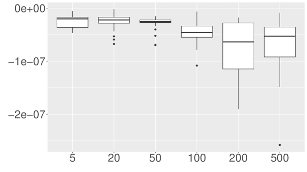
(a) $\ell_{2}$-norm

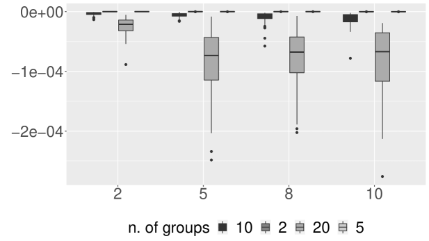
(b) group $\ell_{2}$-norm

Figure 1: Box plots of the difference between the analytical dual norm and that obtained by running Algorithm 1 over $50$ replications of random vectors of varying dimension (for the $\ell_{2}$-norm) and varying group-length and number of groups (for the group $\ell_{2}$-norm).

Figure 2: Box plots of the difference between the $\Omega_{OG}(\mathbf{x})$ dual norm obtained by running Algorithm 1 over $50$ replications of random vectors of varying dimension and varying group-length and number of groups.

4 Application

In this application we consider the dual norm of overlap group $\ell_{2}$-norm, $\Omega_{OG}(\mathbf{x})$ introduced by Bernardi et al., (2021) for kernel penalization in the functional regression context. The norm is defined as

$$\Omega^{c}_{\cal I}(u_{\mathcal{I}^{c}})=\sum_{b\in{\cal B}^{c}}\|c_{b}^{({\cal I}^{c})}\odot u_{\mathcal{I}^{c}}\|_{2},$$ (28)

where ${\cal B}\subset\{1,\dots,B,B+1\}$ is the set of indices of the true non-zero groups and ${\cal I}\subset\{(m,l):m=1,\dots,M;\,l=1,\dots,L\}$ is the set of the indices of the non-zero coefficients $\psi_{m,l}$, $c_{b}=\mathsf{vec}(\mathbf{S}_{b}\odot\mathbf{C})$, where $\mathbf{S}_{b}$ is the $M\times L$ selection matrix with general entry $s_{m,l}^{(b)}$, defined as $1$ if the parameter $\psi_{m,l}$ belongs to group $b$ and 0 otherwise and $\mathbf{C}$ is the matrix with general element $c_{m,l}$ defined as $c_{ml}=\big{(}\sum_{b=1}^{B+1}s_{m,l}^{(b)}\big{)}^{-1}$.

To check for the irrepresentable condition condition, we need to calculate the dual norm $\big{(}\Omega^{c}_{\cal B}\big{)}^{*}\big{(}{\mathbf{Z}}_{0}^{\intercal}{\mathbf{Z}}_{1}({\mathbf{Z}}_{1}^{\intercal}{\mathbf{Z}}_{1})^{-1}\mathbf{r}_{1}\big{)}$, where $\mathbf{r}_{1}$ is the vector containing, for $(m,l)\in\cal I$, the elements $\psi_{m,l}c^{2}_{m,l}\sum_{b\in{\cal B},b:\psi_{b}\ni\psi_{m,l}}\|c_{b}\odot\mbox{\boldmath$\psi$}\|_{2}^{-1}$.

5 Conclusion

In this paper we provide a new algorithm for solving numerically the dual norm optimization problem. The methods relies on the Majorization-Minimization principle of Lange, (2016) combined with barrier methods that efficiently convert a constrained optimization problem into an unconstrained one. Extensive simulation experiments have been performed in order to verify the correctness of operation, and evaluate the performance of the proposed method. Our results demonstrate the effectiveness of the algorithm in retrieving the dual norm even for large dimensions.

References

• Bach et al., (2012) Bach, F., Jenatton, R., Mairal, J., and Obozinski, G. (2012). Optimization with sparsity-inducing penalties. Foundations and Trends® in Machine Learning, 4(1):1–106.
• Bernardi et al., (2021) Bernardi, M., Canale, A., and Stefanucci, M. (2021). Locally sparse function on function regression.
• Boyd et al., (2011) Boyd, S., Parikh, N., Chu, E., Peleato, B., and Eckstein, J. (2011). Distributed optimization and statistical learning via the alternating direction method of multipliers. Foundations and Trends® in Machine Learning, 3(1):1–122.
• Bühlmann and van de Geer, (2011) Bühlmann, P. and van de Geer, S. (2011). Statistics for high-dimensional data. Springer Series in Statistics. Springer, Heidelberg. Methods, theory and applications.
• Hoerl and Kennard, (2000) Hoerl, A. E. and Kennard, R. W. (2000). Ridge regression: Biased estimation for nonorthogonal problems. Technometrics, 42(1):80–86.
• Hunter and Lange, (2004) Hunter, D. R. and Lange, K. (2004). A tutorial on MM algorithms. Amer. Statist., 58(1):30–37.
• Jenatton et al., (2011) Jenatton, R., Audibert, J.-Y., and Bach, F. (2011). Structured variable selection with sparsity-inducing norms. The Journal of Machine Learning Research, 12:2777–2824.
• Lange, (2010) Lange, K. (2010). Numerical analysis for statisticians. Statistics and Computing. Springer, New York, second edition.
• Lange, (2013) Lange, K. (2013). Optimization, volume 95 of Springer Texts in Statistics. Springer, New York, second edition.
• Lange, (2016) Lange, K. (2016). MM optimization algorithms. Society for Industrial and Applied Mathematics, Philadelphia, PA.
• Lange et al., (2014) Lange, K., Chi, E. C., and Zhou, H. (2014). A brief survey of modern optimization for statisticians. International Statistical Review, 82(1):46–70.
• Luenberger and Ye, (2021) Luenberger, D. G. and Ye, Y. ([2021] ©2021). Linear and nonlinear programming, volume 228 of International Series in Operations Research & Management Science. Springer, Cham, fifth edition.
• Nocedal and Wright, (2006) Nocedal, J. and Wright, S. J. (2006). Numerical optimization. Springer Series in Operations Research and Financial Engineering. Springer, New York, second edition.
• Osborne et al., (2000) Osborne, M. R., Presnell, B., and Turlach, B. A. (2000). On the LASSO and its dual. J. Comput. Graph. Statist., 9(2):319–337.
• Sun et al., (2017) Sun, Y., Babu, P., and Palomar, D. P. (2017). Majorization-minimization algorithms in signal processing, communications, and machine learning. IEEE Transactions on Signal Processing, 65(3):794–816.
• Tibshirani, (1996) Tibshirani, R. (1996). Regression shrinkage and selection via the lasso. Journal of the Royal Statistical Society: Series B (Methodological), 58(1):267–288.
• Wu and Lange, (2010) Wu, T. T. and Lange, K. (2010). The MM alternative to EM. Statist. Sci., 25(4):492–505.
• Yuan and Lin, (2006) Yuan, M. and Lin, Y. (2006). Model selection and estimation in regression with grouped variables. J. R. Stat. Soc. Ser. B Stat. Methodol., 68(1):49–67.
• Zhao and Yu, (2006) Zhao, P. and Yu, B. (2006). On model selection consistency of lasso. Journal of Machine Learning Research, 7(90):2541–2563.
• Zou and Hastie, (2005) Zou, H. and Hastie, T. (2005). Addendum: “Regularization and variable selection via the elastic net” [J. R. Stat. Soc. Ser. B Stat. Methodol. 67 (2005), no. 2, 301–320; mr2137327]. J. R. Stat. Soc. Ser. B Stat. Methodol., 67(5):768.