Semiclassical WKB Problem for the non-self-adjoint Dirac operator with an analytic rapidly oscillating potential

Abstract.

In this paper we examine the semiclassical behavior of the scattering data of a non-self-adjoint Dirac operator with a rapidly oscillating potential that is complex analytic in some neighborhood of the real line. Some of our results are rigorous and quite general. On the other hand, complete and concrete understanding requires the investigation of the WKB geometry of specific examples. For such detailed computations we use a particular example that has been investigated numerically more than 20 years ago by Bronski and Miller and rely heavily on their numerical computations. Mostly employing the exact WKB method, we provide the complete rigorous uniform semiclassical analysis of the Bohr-Sommerfeld condition for the location of the eigenvalues across unions of analytic arcs as well as the associated norming constants. For the reflection coefficient as well as the eigenvalues near 0 in the spectral plane, we employ instead an older theory that has been developed in great detail by Olver. Our analysis is motivated by the need to understand the semiclassical behaviour of the focusing cubic NLS equation with initial data $A\exp\{iS/\epsilon\}$, in view of the well-known fact discovered by Zakharov and Shabat that the spectral analysis of the Dirac operator enables the solution of the NLS equation via inverse scattering theory.

1. Introduction

1.1. Motivation

Consider the semiclassical limit ($\epsilon\downarrow 0$) of the solution to the initial value problem of the one-dimensional nonlinear Schrödinger equation with cubic nonlinearity

$$\left\{\begin{array}[]{l}i\epsilon\partial_{t}\psi+\frac{\epsilon^{2}}{2}\partial_{x}^{2}\psi+|\psi|^{2}\psi=0,\quad(x,t)\in{\mathbb{R}}\times{\mathbb{R}}\\ \psi(x,0)=A(x)\exp\{iS(x)/\epsilon\},\quad x\in{\mathbb{R}}\end{array}\right.$$ (1.1)

where $A$ and $S$ are real valued integrable functions defined on the real line.

According to the seminal discovery in [28], this initial value problem can be studied via the so-called inverse scattering method. In order for one to do so, the first ingredient is the $direct$ spectral and scattering analysis of the associated Dirac (or Zakharov-Shabat) operator $\mathfrak{D}_{\epsilon}$ given by

$$\mathfrak{D}_{\epsilon}=\begin{bmatrix}-\frac{\epsilon}{i}\frac{d}{dx}&-iA(x)\exp\{iS(x)/\epsilon\}\\ -iA(x)\exp\{-iS(x)/\epsilon\}&\frac{\epsilon}{i}\frac{d}{dx}\end{bmatrix}.$$

Our main goal in this paper is to provide a rigorous investigation of the semiclassical behavior of the scattering data (reflection coefficient, eigenvalues and their associated norming constants) for the operator $\mathfrak{D}_{\epsilon}$ and apply our conclusions to the semiclassical investigation of the solutions to the focusing NLS equation.

We are interested in $A(x)$ and $S(x)$ that are real analytic functions which can be extended holomorphically to at least a region in the whole complex plane . Although a good deal of our analysis will be fairly general, we will eventually focus on a very particular choice of $A(x)$ and $S(x)$ so that we have a concrete configuration of the geometry of turning points and Stokes lines. Our model will be the $A(x)=S(x)=\sech(2x)$ since this has been the first case considered in detail: a very careful numerical analysis of the eigenvalue problem was done by Bronski [1] in $1996$ and a first investigation of the formal WKB theory, involving numerical computations of turning points and Stokes lines, was conducted by Miller [22] in $2001$. Another model has been studied numerically recently in [18]; there, the authors use $A(x)=30/(1+x^{4})$ and $S(x)=15x^{2}$.

If the parameter $\epsilon$ is not too small, then of course the solution is described by a nonlinear superposition of breathers (corresponding to purely imaginary eigenvalues of $\mathfrak{D}_{\epsilon}$), traveling solitons (corresponding to all other eigenvalues of $\mathfrak{D}_{\epsilon}$) and a background radiation contribution (corresponding to the continuous spectrum of $\mathfrak{D}_{\epsilon}$). This is in a sense the content of the inverse scattering method.

On the other hand, as $\epsilon\downarrow 0$, the solution attains a special form which in particular regions attains a highly oscillatory behavior. Often in such problems one expects the validity of the so-called finite gap ansatz for the semiclassical asymptotics.

Finite Gap Ansatz.

Let $(x_{0},t_{0})$ be a generic point with $x_{0}\in\mathbb{R}$ and $t_{0}>0$. The solution $\psi$ of (1.1) is asymptotically ($\epsilon\downarrow 0$) described (locally) as a slowly modulated $G$ phase wavetrain. More precisely, setting $x=x_{0}+\epsilon\hat{x}$ and $t=t_{0}+\epsilon\hat{t}$ (so that $x_{0},t_{0}$ are “slow” variables while $\hat{x},\hat{t}$ are “fast” variables), there exist parameters (all of which depend on the slow variables $x_{0}$, $t_{0}$ but not on $\hat{x},\hat{t}$)

• $a,U_{0},k_{0},w_{0}$ in ${\mathbb{C}}$ and

• ${\bf U}=[U_{1},\dots,U_{G}]^{T}$, ${\bf k}=[k_{1},\dots,k_{G}]^{T}$, ${\bf w}=[w_{1},\dots,w_{G}]^{T}$, ${\bf Y}=[Y_{1},\dots,Y_{G}]^{T}$, ${\bf Z}=[Z_{1},\dots,Z_{G}]^{T}$ in ${\mathbb{C}}^{G}$

such that as $\epsilon\downarrow 0$,

$$\psi(x,t)=\psi(x_{0}+\epsilon\hat{x},t_{0}+\epsilon\hat{t}\hskip 2.0pt)$$

has the following leading order asymptotics

$$\psi(x,t)\sim a(x_{0},t_{0})\exp\Big{\{}i\Big{(}\tfrac{U_{0}(x_{0},t_{0})}{\epsilon}+k_{0}(x_{0},t_{0})\hat{x}-w_{0}(x_{0},t_{0})\hat{t}\Big{)}\Big{\}}\\ \cdot\frac{\Theta\bigg{(}{\bf Y}(x_{0},t_{0})+i\Big{(}\frac{{\bf U}(x_{0},t_{0})}{\epsilon}+{\bf k}(x_{0},t_{0})\hat{x}-{\bf w}(x_{0},t_{0})\hat{t}\Big{)}\bigg{)}}{\Theta\bigg{(}{\bf Z}(x_{0},t_{0})+i\Big{(}\frac{{\bf U}(x_{0},t_{0})}{\epsilon}+{\bf k}(x_{0},t_{0})\hat{x}-{\bf w}(x_{0},t_{0})\hat{t}\Big{)}\bigg{)}}.$$ (1.2)

All parameters here are defined in terms of an underlying Riemann surface $X$ which depends solely on $x_{0},t_{0}$. The moduli of $X$ vary slowly with $x,t$, i.e. they depend on $x_{0},t_{0}$ but not on $\epsilon,\hat{x},\hat{t}$. $\Theta$ is the G-dimensional Jacobi theta function associated with $X$. The genus of $X$ can vary with $x_{0},t_{0}$. In fact, the $(x,t)$-plane is divided into open regions in each of which G is constant.

On the boundaries of such regions (sometimes called “caustics”; they are unions of analytic arcs), some degeneracies appear in the mathematical analysis (we may have “pinching” of the surfaces $X$ for example).

The above formula (1.2) gives asymptotics which is pointwise in $x,t$. We refer to [19] and [20], for the justification of the above “finite gap” formula in the case of special “bell-like” initial data $A(x)$ [and $S(x)=0$], as well as the exact formulae for the parameters and the definition of the theta functions. The formula is actually uniformly valid in compact $(x,t)$-sets not containing points on the caustics. The mathematical theory leading to the asymptotic formula is the well-known non-linear steepest descent method. Near the caustics, boundary layers separating regions of different genus appear. For an analysis of the somewhat more delicate behavior (especially for higher order terms in $\epsilon$) near the first caustic one can consult [5].

The following two pictures (prepared for us by Nikos Efremidis) exemplify this behavior in two separate cases. In both cases $A(x)=2\sech x$; but in the first picture $S$ is identically 0 while in the second one $S(x)=\sech x$. Here $\epsilon=0.1$ and the time is actually rescaled (divided by 0.1). We only show plots for $|\psi|^{2}$.

One observes the following:

• There is no qualitative difference between the two cases, at least for not very large times.

• The behavior of the solution is quite different in three distinct regions in the $(x,t)$-plane.

• In the first region (for smaller times t) things are fairly “smooth”. There are no oscillations. In the intermediate region fast oscillations appear. The curve separating these two regions appears to be fairly continuous. There is also a third region where the nature of the fast oscillations changes. Again the intermediate and third regions are separated by a seemingly continuous curve.

Figure 1. A solution of the initial value problem (1.1) for $\epsilon=0.1$ with initial data $\psi(x,0)=2\sech x$ [i.e. $A(x)=2\sech x$ and $S(x)=0$]. In this figure $|\psi|^{2}(x,t)$ is being plotted. The horizontal axis represents $x$ while $t$ runs on the vertical axis (as shown on the left). The bar on the right of the plot shows a graduated scale for the values of $|\psi|^{2}$ ranging from deep black (where $|\psi|^{2}$ is small) to bright white (where $|\psi|^{2}$ is big).

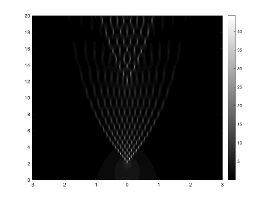
Figure 2. A solution of the initial value problem (1.1) for $\epsilon=0.1$ with initial data $\psi(x,0)=2(\sech x)\exp\big{\{}\tfrac{\sech x}{0.1}\big{\}}$ [i.e. $A(x)=2\sech x$ and $S(x)=\sech x$]. The figure shows the plot of $|\psi|^{2}(x,t)$. On the horizontal axis lies $x$ while $t$ runs on the vertical axis (as shown on the left). Also on the right of the plot there is a bar showing a graduated scale for the values of $|\psi|^{2}$ ranging from deep black (where $|\psi|^{2}$ is small) to bright white (where $|\psi|^{2}$ is big).

In [19] we have been able to identify the first region in Figure 1 with the genus 0 region. The intermediate region is the genus 2 region and then comes the genus 4 region. The separating curves are the “caustics”. In principle, there can be a very large number of such caustics. But it is also worth pointing out that the $2\sech x$ data, being a nonlinear superposition of many (of order $\epsilon^{-1}$) breathers, is actually periodic in time with period $\mathcal{O}(\epsilon^{-1})$. Of course, this is not seen in our picture, since what happens at such large times is not shown.

If we were to run our numerics in Figure 2 for larger times, we would also observe many separated traveling solitons at different non-zero speeds, since (as we shall see later) the initial data give rise to many eigenvalues with non-zero real part.

The question of the semiclassical approximation of the scattering data has a deeper significance in view of the instabilities of the problem which apper in many levels. In fact even in the non-semiclassical regime, the focusing NLS is the main model for the so-called “modulational instability” (see [3] and [4]), although for positive fixed $\epsilon$ the initial value problem is well-posed. Semiclassically the instabilities become more pronounced. One way to see this, is related to the underlying ellipticity of the formal semiclassical limit. To be more specific, consider the well-known Madelung transformation (see [21])

$$\begin{cases}\rho=|\psi|^{2}\\ \mu=\epsilon\Im(\psi^{*}\psi_{x})\end{cases}$$

where $\psi^{*}$ denotes the complex conjugate of $\psi$. Then the initial value problem (1.1) becomes

$$\begin{cases}\rho_{t}+\mu_{x}=0\\ \mu_{t}+\Big{(}\frac{\mu^{2}}{\rho}+\frac{\rho^{2}}{2}\Big{)}_{x}=\frac{\epsilon^{2}}{4}\partial_{x}[\rho(\log\rho)_{xx}]\\ \rho(x,0)=A^{2}(x)\\ \mu(x,0)=A^{2}(x)S^{\prime}(x).\end{cases}$$

The formal limit, as $\epsilon\downarrow 0$, is

$$\begin{cases}\rho_{t}+\mu_{x}=0\\ \mu_{t}+\Big{(}\frac{\mu^{2}}{\rho}+\frac{\rho^{2}}{2}\Big{)}_{x}=0\\ \rho(x,0)=A^{2}(x)\\ \mu(x,0)=A^{2}(x)S^{\prime}(x).\end{cases}$$

This is an initial value problem for an elliptic system of equations; and so one expects that small perturbations of the initial data (independent of $\epsilon$) can lead to large changes in the solution at any given time.

Instabilities also appear, independently, at the spectral analysis of the related non-self-adjoint Dirac operator: indeed, small changes of the potential are expected to result in relatively large changes in the discrete spectrum; this is not true when the phase $S=0$ but it is true otherwise. We refer to [2] for a numerical investigation of this fact in the special case $A(x)=S(x)=sech(2x)$ and to [8] for the discussion of the more general phenomenon in the theory of pseudo-differential operators. Instabilities are evident also at the related equilibrium measure problem (it is a “max-min” problem; see [20]), the related Whitham equations (they are also elliptic) and even in the numerical studies of the problem. What was initially called the modulational instability is just the tip of the iceberg!

One might even question whether the whole project is worthwhile studying in detail, at least as a valid physical model, in view of all these instabilities. To this, a first response is that the semiclassical analysis turns out in practice to be relevant even for not so small values of the semi-classical parameter $\epsilon$ (for example in applications to nonlinear optics). From a mathematical point of view, it is a fascinating instance of a difficult unstable problem that can be approximated by solvable stable problems; this approximation is very singular and non-trivial and its study involves important connections to different areas of mathematics (namely PDE theory, spectral theory of non-self-adjoint operators, WKB analysis, potential theory (cf. [20]), Riemann surface theory, hydrodynamic instability theory).

Going back to the pictures presented above, in the first (genus 0) region there are no fast oscillations and actually strong semiclassical limits exist for both $\rho$ and $\mu$. They actually satisfy the formally limiting PDE. In the other (higher genus) regions, violent oscillations of frequency order $\epsilon^{-1}$ appear and a strong pointwise limit does not exist. But to the extent that we can perform a full asymptotic analysis, both at the direct scatterring and the inverse scattering stage, we can show that there is at least a weak limit and we are able to provide complete asymptotic formulae (as above).

The semiclassical analysis of the NLS solution $\psi$ in [19] undertook the asymptotic ($\epsilon\downarrow 0$) analysis of the inverse scattering problem, to which Zakharov and Shabat have reduced the solution of the equation; in particular, we worked on the formulation of that problem as a Riemann-Hilbert factorisation problem and we applied and extended ideas and calculations going back to the seminal work of Deift, Venakides and Zhou ([6], [7]). But no careful semiclassical analysis of the $direct$ scattering problem had been undertaken until recently. Instead, an ad hoc approximation of the eigenvalues by their Bohr-Sommerfeld approximants was used as a starting point (and the reflection coefficient was set identically to 0, in the same formal spirit).

In [14] the rigorous semiclassical analysis of the scattering data of the related Dirac (or Zakharov-Shabat) operator was completed in the case where $A$ is real analytic, integrable, positive, symmetric, with only one local maximum (and where for simplicity the second derivative of $A$ is non-zero). We applied the so-called exact WKB theory, which will also be applied in the present work.

In [15] the analyticity assumption was replaced by a mild smoothness assumption and a different method was employed, going back to Langer and Olver [23]. In a sequel [16], the general case with several local maxima and minima was also completed, under the assumption that potentials are smooth and positive. In all the above cases the initial phase $S(x)$ is identically zero. Of course, even with an initial phase zero, the Madelung system above shows that a non-trivial phase will appear immediately for any small time $t$. But it is also reasonable to postulate a non-zero initial phase especially in cases where the discrete spectrum is no more imaginary and the instability due to the non-self-adjointness of the Dirac operator is instrumental.

The exact WKB method was first developed for the Schrödinger operator, but here we apply it to the Dirac operator that is associated to the focusing NLS equation. The method goes back to works of Ecalle [9] and Voros [27] but here we argue along the lines of the papers of Gérard-Grigis [13] and Fujiié-Lasser-Nédélec [10]. Rather than relying on the usual formal WKB method which relies on asymptotic series that are in general divergent, we use a “resummation” of the series and in fact construct “exact solutions” in terms of convergent series, thus resolving a problem of “asymptotics beyond all orders”.

For the study of the eigenvalues with small imaginary part, the exact WKB method seems to break down and Olver’s [23] is not directly applicable since we don’t know a priori that the eigenvalues are purely imaginary (as in [15]). Fortunately the somewhat forgotten paper [24] which generalizes his earlier work is proved to be useful here.

1.2. Organization of the paper

The plan of this paper is the following. In the next section we investigate the eigenvalues of the Dirac operator that in the semiclassical limit lie away from the real axis. In §2.1, we present the main ideas that will be used in the following sections, including the definition of turning points, progressive paths, Stokes lines, admissible contours and asymptotic spectral arcs. In §2.2, we introduce the theory of the exact (resummed and converging) WKB solutions and state a basic theorem about convergence and semiclassical asymptotics. Then in §2.3 we prove a theorem that shows how different solutions are connected in a neighborhood of a simple turning point. We use it in §2.4, to give a rigorous justification of the Bohr-Sommerfeld asymptotic conditions for the location of the eigenvalues that lie away from the bifurcation point (see Figure 10). In §2.5 we refine the exact WKB analysis in a small neighborhood of a bifurcation point. In the last section of this paragraph, namely §2.6, we apply all the results above to the particular case $A(x)=S(x)=\sech(2x)$, where we make heavy use of the numerical results and figures of [22].

We are not able at this point to extend the exact WKB method for the eigenvalues near $0$. In paragraph 3, we use instead Olver’s theory as it was extended in [24]. We start in §3.1 with some preparatory material and move to §3.2 where we encounter the behavior of solutions near a simple turning point (compare this with §2.3). Next, comes §3.3 where we present asymptotics for the error-terms in our solutions. The connection of the above solutions -in the way of Olver- is achieved in §3.4. Using the asymptotics for the error-terms, we arrive at the asymptotic form of these connection formulas in §3.5. We then assemble all the previous results, and in §3.6 we provide a Bohr-Sommerfeld quantization condition for the location of the eigenvalues that lie near zero.

In paragraph 4 we are interested in the behavior of the corresponding norming constants to the eigenvalues discussed previously. Then in paragraph 5, we use Olver’s method as exploited in [15], to study the behavior of the reflection coefficient; we prove that it is small away from the point 0 (in the spectral real line) in §5.1. Also, in §5.2, we give asymptotics for the reflection coefficient nearer to zero.

Finally, in paragraph 6, we present the application of the WKB results to the focusing NLS problem and explain how the analysis of [19], [20] extends to our present case in view of these results.

Since the approximation technique we are using for the near-zero eigenvalues relies on modified Bessel functions, we have included in the appendix a paragraph that contains all the material that we shall need.

1.3. Notation

Before we start our main exposition, we specify some notation used throughout our work.

• The symbol ${\mathbb{N}}_{0}$ is used for the set ${\mathbb{N}}\cup\{0\}$.

• The Riemann sphere is denoted by $\overline{{\mathbb{C}}}={\mathbb{C}}\cup\{\infty\}$.

• The (topological) closure of a set $S\subseteq\overline{C}$ shall be denoted by $\textsf{clos}(S)\subseteq\overline{C}$.

• We use the notation ${\mathbb{R}}^{\pm}=\{\,x\in{\mathbb{R}}\mid\pm x>0\,\}$ for the sets of positive/negative numbers.

• Complex conjugation is denoted with a star superscript, $*$; i.e. $z^{*}$ is the complex conjugate of $z$.

• The transpose of a matrix $M$ is denoted by $M^{T}$.

• For the upper half-plane we write $\mathbb{H}^{+}=\{\,z\in{\mathbb{C}}\mid\Im z>0\,\}$.

• For a set $\Sigma\subseteq{\mathbb{R}}$, when we write $i\Sigma$ we mean the set $\{i\kappa\mid\kappa\in\Sigma\}\subset{\mathbb{C}}$. Also, for $z_{1},z_{2}\in{\mathbb{C}}$ the set $[z_{1},z_{2}]\subset{\mathbb{C}}$ denotes the closed line segment starting at $z_{1}$ and ending at $z_{2}$.

• The set of holomorphic functions from a domain $A$ to a domain $B$ shall be denoted by $\mathscr{H}(A;B)$. For the holomorphic functions from $A$ to ${\mathbb{C}}$, we simply write $\mathscr{H}(A)$.

• The symbol $\sigma(a\rightsquigarrow b)$ is used to denote a curve in ${\mathbb{C}}$, parametrized by $\sigma$, starting at $a$ and ending at $b$.

• Let ${\mathcal{W}}[\textbf{f},\textbf{g}]$ be defined as the determinant of the $2\times 2$ matrix $[\textbf{f}\hskip 3.0pt\textbf{g}]$ consisting of the two column vectors f, $\textbf{g}\in{\mathbb{C}}^{2}$.

• The wronskian of the pair $\{f,g\}$ of functions is represented by $W[f,g]$.

• For a continuous function $f$ in ${\mathbb{R}}$, the notation $\int f(t)dt$ denotes any of its primitives.

• If $z\in{\mathbb{C}}$, we denote by $\text{ph}z\in(-\pi,\pi]$ its phase.

• The abbreviations LHS and RHS stand for left-hand side and right-hand side respectively.

• EV and EF stand for eigenvalues and eigenfunctions respectively.

• The acronym MBF means modified Bessel function.

2. Eigenvalues Away From The Real Axis

2.1. General strategy

This paragraph presents a general scheme (see [22], and also [11] for the case of Schrödinger operators) for finding the semiclassical EVs of the Dirac (or Zakharov-Shabat) operator

$$\mathfrak{D}_{\epsilon}=\begin{bmatrix}-\frac{\epsilon}{i}\frac{d}{dx}&\omega(x,\epsilon)\\ -\omega^{*}(x,\epsilon)&\frac{\epsilon}{i}\frac{d}{dx}\end{bmatrix}$$ (2.1)

where $\omega$ is the complex potential function

$$\omega(x,\epsilon)=-iA(x)\exp\Big{\{}i\frac{S(x)}{\epsilon}\Big{\}}$$

for some real-valued, analytic functions $A(x)$ and $S(x)$ defined on the real line [$\omega^{*}(x,\epsilon)$ represents the complex conjugate of $\omega(x,\epsilon)$] such that $A$, $S$ and $S^{\prime}$ are integrable. As previously stated in the introduction, we shall be interested in the spectral (generalized eigenvalue) problem

$$\mathfrak{D}_{\epsilon}\textbf{u}=\lambda\textbf{u}$$ (2.2)

where $\textbf{u}=[u_{1}\hskip 3.0ptu_{2}]^{T}$ is a function from ${\mathbb{R}}$ to ${\mathbb{C}}^{2}$ and $\lambda\in\mathbb{C}$ plays the role of the spectral parameter.

The operator $\mathfrak{D}_{\epsilon}$ is non-self-adjoint and the eigenvalues are distributed in the complex plane. But in the semiclassical limit, their location is restricted close to the numerical range $\mathcal{R}$ of the semiclassical symbol.

We shall see [see the reasoning that follows, eventually leading to (2.7)] that the eigenvalues of $\mathfrak{D}_{\epsilon}$ coincide with those of the operator

$$\begin{bmatrix}-\frac{\epsilon}{i}\frac{d}{dx}-\frac{1}{2}S^{\prime}(x)&-iA(x)\\ -iA(x)&\frac{\epsilon}{i}\frac{d}{dx}-\frac{1}{2}S^{\prime}(x)\end{bmatrix}.$$ (2.3)

We have the following definition.

Definition 2.1.

The numerical range $\mathcal{R}$ of the symbol

$$\begin{bmatrix}-\xi-\frac{1}{2}S^{\prime}(x)&-iA(x)\\ -iA(x)&\xi-\frac{1}{2}S^{\prime}(x)\end{bmatrix}$$

of the matrix/operator in (2.3) is defined to be the union of the set of values of the eigenvalues $-\frac{1}{2}S^{\prime}(x)\pm\sqrt{\xi-A(x)^{2}}$ of this matrix when $(x,\xi)$ varies in the whole phase space ${\mathbb{R}}^{2}$.

We see that

$$\mathcal{R} ={\mathbb{R}}\cup{\mathcal{R}}_{0}\quad\text{where}\quad$$

$${\mathcal{R}}_{0} =-\frac{1}{2}\Big{[}\inf_{x\in{\mathbb{R}}}S^{\prime}(x),\sup_{x\in{\mathbb{R}}}S^{\prime}(x)\Big{]}\times\Big{[}-\sup_{x\in{\mathbb{R}}}|A(x)|,\sup_{x\in{\mathbb{R}}}|A(x)|\Big{]}.$$ (2.4)

The following result concerning the semiclassical eigenvalues is well-known; see e.g. [8].

Proposition 2.2.

For any compact set $K\subset{\mathbb{R}}^{2}$ with $K\cap{\mathcal{R}}_{0}=\emptyset$, there exists $\epsilon_{0}>0$ such that there is no eigenvalue in $K$ for $0<\epsilon<\epsilon_{0}$.

It is clear that (2.2) can be written equivalently as a first order system of differential equations, namely

$$\frac{\epsilon}{i}\frac{d}{dx}\textbf{u}(x,\lambda,\epsilon)=K(x,\lambda,\epsilon)\textbf{u}(x,\lambda,\epsilon)$$ (2.5)

where

$$K(x,\lambda,\epsilon)=\begin{bmatrix}-\lambda&\omega(x,\epsilon)\\ \omega^{*}(x,\epsilon)&\lambda\end{bmatrix}.$$ (2.6)

Applying first the transformation

$$\textbf{u}(x,\lambda,\epsilon)=\begin{bmatrix}\exp\big{\{}i\frac{S(x)}{2\epsilon}\big{\}}&0\\ 0&\exp\big{\{}-i\frac{S(x)}{2\epsilon}\big{\}}\end{bmatrix}\tilde{\textbf{v}}(x,\lambda,\epsilon)$$

where $\tilde{\textbf{v}}=[\tilde{v}_{1}\hskip 3.0pt\tilde{v}_{2}]^{T}$, takes the system in (2.5) to a new form

$$\frac{\epsilon}{i}\frac{d}{dx}\tilde{\textbf{v}}(x,\lambda,\epsilon)=\begin{bmatrix}-\lambda-\frac{1}{2}S^{\prime}(x)&-iA(x)\\ iA(x)&\lambda+\frac{1}{2}S^{\prime}(x)\end{bmatrix}\tilde{\textbf{v}}(x,\lambda,\epsilon)$$ (2.7)

where prime denotes differentiation with respect to $x$. Next, we apply the mapping

$$\tilde{\textbf{v}}(x,\lambda,\epsilon)=\begin{bmatrix}1&1\\ -1&1\end{bmatrix}\textbf{v}(x,\lambda,\epsilon)$$

where $\textbf{v}=[v_{1}\hskip 3.0ptv_{2}]^{T}$, to finally express the initial system as

$$\frac{\epsilon}{i}\frac{d}{dx}\textbf{v}(x,\lambda,\epsilon)=M(x,\lambda)\textbf{v}(x,\lambda,\epsilon)$$ (2.8)

where

$$M(x,\lambda)=\begin{bmatrix}0&g_{+}(x,\lambda)\\ -g_{-}(x,\lambda)&0\end{bmatrix}$$ (2.9)

$$\text{and}\quad g_{\pm}(x,\lambda)=\mp[\lambda+\frac{1}{2}S^{\prime}(x)\pm iA(x)].$$ (2.10)

The important function to study is

$$V_{0}(x,\lambda) =\det M(x,\lambda)$$

$$=g_{-}(x,\lambda)g_{+}(x,\lambda)$$

$$=-[\lambda+\tfrac{1}{2}S^{\prime}(x)]^{2}-A^{2}(x).$$ (2.11)

The zeros of this function play an important role. So we state the following definition.

Definition 2.3.

For a fixed value of $\lambda\in\mathbb{C}$, the zeros of $V_{0}(\cdot,\lambda)$ in $\mathbb{C}$ are called turning points of (2.8).

In our application, the potential function $V_{0}(\cdot,\lambda)$ in (2.1), i.e.

$$V_{0}(x,\lambda)=-[\lambda+\tfrac{1}{2}S^{\prime}(x)]^{2}-A^{2}(x)$$

is complex-valued for $\lambda\in{\mathbb{C}}\setminus{\mathbb{R}}$ and the turning points are in general complex. Assuming that the functions $A(x)$ and $S(x)$ extend analytically to some fixed complex neighborhood $\Omega_{0}$ of the real axis, we may consider the asymptotics of solutions of (2.5) [eventually of (2.8)] on some contour (in the complex $x$-plane), other than the real $x$-axis, connecting $-\infty$ to $+\infty$ and forcing that contour to pass through at least one pair of complex turning points.

Let us define

$$z(x,\lambda,\alpha)=i\int_{\gamma(\alpha\rightsquigarrow x)}\sqrt{-V_{0}(t,\lambda)}dt$$

for a fixed point $\alpha\in\Omega_{0}$.

Definition 2.4.

A path $\gamma$ in $\Omega_{0}$ along which $\Re z$ is strictly monotone will be called a progressive path.

Remark 2.5.

This notion does not depend on the branch of the square root nor the base point $\alpha$. This is equivalent to $\gamma$ been transversal to the Stokes curves defined later in Definition 2.6. When the branch of the square root and the orientation of the path are specified, we also say a path is $+$-progressive (resp. $-$-progressive) if $\Re z$ is strictly increasing (resp. decreasing).

It is important to notice that, in our setting where $S^{\prime}$ and $A$ tend to 0 at infinity, $\sqrt{-V_{0}(t,\lambda)}$ tends to $\pm\lambda$. Hence if $\Im\lambda$ is non-zero, then the real axis is progressive near infinity.

The level curves of $\Re[z(x,\lambda,\alpha)]$ in the complex $x$-plane are very important for what follows. Indeed, $(\pm)$-progressive curves are always transversal to those. For that, they deserve a definition.

Definition 2.6.

The level curves of $\Re[z(x,\lambda,\alpha)]$ in the complex $x$-plane are called the Stokes lines (or Stokes curves) of the system (2.8).

The geometric configuration of the Stokes curves is crucial in the investigation of the domain of validity of the asymptotic expansion of the WKB solutions. Notice that from a simple turning point [i.e. a simple zero of the function $V_{0}(\cdot,\lambda)$ in (2.1)], exactly three Stokes lines emanate. At such a point, the angles between two Stokes curves are all $2\pi/3$.

Fix $\lambda\in{\mathbb{C}}\setminus{\mathbb{R}}$. With the above intuition in mind, we have the following definition.

Definition 2.7.

Let $\{x_{-}(\lambda)$, $x_{+}(\lambda)\}$ be a pair of simple complex roots of $V_{0}(x,\lambda)=0$. A contour $C=C^{-}\cup C^{0}\cup C^{+}$ in $\Omega_{0}$ shall be called admissible if the following four conditions hold true:

• $V_{0}$ is holomorphic in $x$, in the region of the complex $x$-plane enclosed by $C$ and the real $x$-axis (this is needed to ensure that the approximate eigenfunctions can be continued back to the real $x$-axis).

• The contour $C^{-}$ is a progressive path from $x_{-}(\lambda)$ to $-\infty$ which coincides with the real axis for $-\Re x\gg 1$.

• The contour $C^{+}$ is a progressive path from $x_{+}(\lambda)$ to $+\infty$ which coincides with the real axis for $\Re x\gg 1$.

• The contour $C^{0}$ is a path from $x_{-}(\lambda)$ to $x_{+}(\lambda)$ along which $\Re z(x,\lambda,x_{-}(\lambda))$ vanishes identically; in other words, $C^{0}$ is a Stokes line.

Remark 2.8.

The term admissible also appears in [22] but here, we impose a stronger requirement on $C^{-}$ and $C^{+}$. This stronger definition is directly applicable to the exact WKB method of the next section, and was first used for the study of quantum resonances of the Schrödinger operator in [11].

Item (iv) in the list above can be reinterpreted as a differential equation for the path $C^{0}$ in the complex $x$-plane. Indeed, if $x=u+iv$, where $u,v\in\mathbb{R}$, then a field of curves is defined by the differential relation

$$\Re\bigg{\{}i\sqrt{-V_{0}(u+iv,\lambda)}(du+idv)\bigg{\}}=0.$$ (2.12)

The idea guiding the definition above is that the set of $\lambda$ for which such admissible contours exist is (hopefully) the locus of points in the complex plane that attracts the actual eigenvalues as $\epsilon\to 0$. This cannot be true in general, as we shall see soon, but an appropriately extented generalisation of this statement probably is. See the last remark 2.25 of this section.

Suppose now that for a pair of complex turning points $\{x_{-}(\lambda),x_{+}(\lambda)\}$ we have the condition

$$\Re\bigg{\{}i\int_{C^{0}(x_{-}(\lambda)\rightsquigarrow x_{+}(\lambda))}\sqrt{-V_{0}(t,\lambda)}dt\bigg{\}}=0$$ (2.13)

and let $\lambda$ vary. Given a pair of turning points depending on $\lambda$ that are distinct throughout a domain in the complex $\lambda$-plane, relation (2.13) itself determines a curve in the complex $\lambda$-plane. If $\lambda$ is on one of these curves, the standard WKB procedure can be expected to apply to determine whether $\lambda$ is in fact an $o(1)$ distance away from an eigenvalue (of course, this is subject to the curve avoiding any singularities and the existence of appropriate progressive paths $C^{-}$, $C^{+}$).

Therefore, as $\epsilon\downarrow 0$, we expect that the discrete eigenvalues of (2.1) will accumulate on the union of curves in the complex $\lambda$-plane described by formula (2.13), with the union being taken over pairs of complex turning points. Hence we are led to the following.

Definition 2.9.

The curves in the complex $\lambda$-plane consisting of $\lambda$-points that give rise to admissible contours $C$ (on the $x$-plane) will be called asymptotic spectral arcs.

Definition 2.10.

The set that is defined as the union of all the asymptotic spectral arcs in the complex $\lambda$-plane will be called the asymptotic spectrum of our Dirac operator.

Remark 2.11.

It follows from the arguments above that this asymptotic spectrum is a union of analytic arcs; if for each $\lambda$ there is only a finite number of turning points, then the asymptotic spectrum is a finite union of asymptotic spectral arcs.

Applying the exact WKB theory stated below in a neighborhood of the contour $C$ (admissible contour), we shall rigorously obtain the eigenvalue approximation by $\lambda$’s satisfying

$$\frac{1}{\pi\epsilon}\Im\bigg{\{}i\int_{C^{0}(x_{-}(\lambda)\rightsquigarrow x_{+}(\lambda))}\sqrt{-V_{0}(t,\lambda)}dt\bigg{\}}-\frac{1}{2}\in\mathbb{Z}$$ (2.14)

which can be interpreted as a Bohr-Sommerfeld quantization rule. Such $\lambda$’s are on the asymptotic spectral arc corresponding to the condition (2.13) for the turning points $x_{-}(\lambda)$ and $x_{+}(\lambda)$.

We remark that, in general, there may well be eigenvalues which are not associated with such an asymptotic spectral arc as defined so far. This is illustrated by the example below.

Example 2.12.

Consider the simplest case where $S(x)$ is linear, i.e. $S^{\prime}(x)=c\in{\mathbb{R}}$ is constant. In this case, the rectangular region ${\mathcal{R}}_{0}$ corresponds to the segment

$${\mathcal{R}}_{0}=\Big{\{}-\frac{c}{2}\Big{\}}\times\Big{[}-\sup_{x\in{\mathbb{R}}}|A|,\sup_{x\in{\mathbb{R}}}|A|\Big{]}.$$

Additionally, if $A(x)$ is “bell-shaped”, i.e. if it decays at $\pm\infty$ and $xA^{\prime}(x)<0$ in ${\mathbb{R}}^{\pm}$, then for any $\lambda$ lying in either of the segments $[-\frac{c}{2},-\frac{c}{2}+i\sup A]$ or $[-\frac{c}{2},-\frac{c}{2}-i\sup A]$, there exist exactly two real, simple turning points $x_{-}(\lambda)$, $x_{+}(\lambda)$ connected by a Stokes line $C^{0}=[x_{-}(\lambda),x_{+}(\lambda)]\subset{\mathbb{R}}$, and $C_{-}=(-\infty,x_{-}(\lambda))$, $C_{+}=(x_{+}(\lambda),+\infty)$ are progressive. Hence $C={\mathbb{R}}$ is an admissible contour and the vertical segments $[-\frac{c}{2},-\frac{c}{2}+i\sup A]$ and $[-\frac{c}{2},-\frac{c}{2}-i\sup A]$ are asymptotic spectral arcs.

Now, if we keep the linearity of $S$ but consider $A(x)$ to be double humped, say $A(x)=[(x^{2}-1)^{2}+1]^{-1}$, the complex intervals $[-\frac{c}{2},\frac{-c+i}{2}]$, $[-\frac{c}{2},\frac{-c-i}{2}]$ are asymptotic spectral arcs just as above. In particular, when $\lambda=\frac{-c\pm i}{2}$, there appears a double turning point at the origin $x=0$ on the Stokes line $C^{0}=[-\sqrt{2},\sqrt{2}]$. However, for $\lambda\neq\frac{-c\pm i}{2}$ in $[\frac{-c+i}{2},-\frac{c}{2}+i]$ or $[\frac{-c-i}{2},-\frac{c}{2}-i]$, $C^{0}$ splits into two Stokes lines, and such $\lambda$ does not belong to the asymptotic spectral arcs according to the above definition (although there do exist eigenvalues near such $\lambda$, see [17]).

But there is no reason why we should not allow two or more Stokes lines apearing in an admissible path. We thus propose the following general definition. We note however that for the specific example we eventually focus on, $A(x)=S(x)=\sech(2x)$, there is at most one Stokes line appearing.

Definition 2.13.

Consider $N\in{\mathbb{N}}$. In general, we call a contour $C$ admissible if the following conditions hold.

• $V_{0}$ is holomorphic in $x$, in the region of the complex $x$-plane enclosed by $C$ and the real $x$-axis.

• $C$ coincides with ${\mathbb{R}}$ outside a compact set.

• $C$ contains a finite number of pairs of simple turning points $x_{-}^{i}(\lambda)$, $x_{+}^{i}(\lambda)$, where $i=1,...,N$, with

  $$V_{0}(x^{i}_{\pm}(\lambda),\lambda)=0,$$

• $C$ consists of a progressive curve $C^{-}$ connecting $-\infty$ and $x_{-}^{1}(\lambda)$, a progressive curve $C^{+}$ connecting $x_{+}^{N}(\lambda)$ and $+\infty$, progressive curves connecting $x^{i}_{+}(\lambda)$ and $x^{i+1}_{-}(\lambda)$ ($i=1,...,N-1$) and Stokes lines connecting $x^{i}_{-}(\lambda)$ and $x^{i}_{+}(\lambda)$, $i=1,...,N$.

Even this more general definition cannot be completely comprehensive as a characterization of eigenvalues, since it does not take into account double truning points, which can exist, at least non-generically, as we will eventually see.

2.2. The exact WKB method

In this and next subsection 2.3, we review the local theory of the exact WKB method applied to our Zakharov-Shabat operator in a fixed open set in ${\mathbb{C}}$.

Let us fix $\lambda$, let $\Omega$ be a simply connected subdomain of the $x$-complex plane free from turning points, and take a fixed point $\alpha\in\Omega$. We define a phase map

$$z(\cdot,\lambda,\alpha):\Omega \rightarrow\mathbb{C}\quad\text{with}$$

$$z(x,\lambda,\alpha)=i\int_{\gamma(\alpha\rightsquigarrow x)} \sqrt{-V_{0}(t,\lambda)}dt$$ (2.15)

where of course the path of integration is irrelevant and we choose the branch of $\sqrt{-V_{0}(x,\lambda)}$ which makes it positive for large $x>0$. Observe that $z$ is uniquely defined in $\Omega$ and it maps $\Omega$ conformally to $z(\Omega,\lambda,\alpha)$.

We look for solutions of (2.8) having the form

$$\textbf{v}(x,\lambda,\epsilon,\alpha)=\exp\bigg{\{}\pm\frac{z(x,\lambda,\alpha)}{\epsilon}\bigg{\}}\tilde{\textbf{w}}^{\pm}[z(x,\lambda,\alpha)]$$ (2.16)

for $\tilde{\textbf{w}}^{\pm}=[\tilde{w}^{\pm}_{1}\hskip 3.0pt\tilde{w}^{\pm}_{2}]^{T}$. Substituting this in (2.8), we get the system

$$\frac{\epsilon}{i}\frac{d}{dz}\tilde{\textbf{w}}^{\pm}(z)=\begin{bmatrix}\pm i&H(z)^{-2}\\ -H(z)^{2}&\pm i\end{bmatrix}\tilde{\textbf{w}}^{\pm}(z)$$ (2.17)

where [upon recalling (2.10)] the function $H$ is given by

$$H(z)=\bigg{[}\frac{g_{-}(x,\lambda)}{g_{+}(x,\lambda)}\bigg{]}^{1/4}.$$

Finally, we set

$$P_{\pm}(z)=\begin{bmatrix}H(z)^{-1}&H(z)^{-1}\\ iH(z)&-iH(z)\end{bmatrix}\begin{bmatrix}0&1\\ 1&0\end{bmatrix}^{\frac{1\pm 1}{2}}$$

and apply the transformation

$$\tilde{\textbf{w}}^{\pm}(z)=P_{\pm}(z)\textbf{w}^{\pm}(z)$$

for $\textbf{w}^{\pm}=[w^{\pm}_{\rm even}\hskip 3.0ptw^{\pm}_{\rm odd}]^{T}$. Then the system in (2.17) is written as

$$\frac{\epsilon}{i}\frac{d}{dz}\textbf{w}^{\pm}(z)=\begin{bmatrix}0&\mathcal{H}(z)\\ \mathcal{H}(z)&\mp\frac{2}{\epsilon}\end{bmatrix}\textbf{w}^{\pm}(z)$$ (2.18)

in which we consider $\mathcal{H}$ to be defined by

$$\mathcal{H}(z)=\frac{\dot{H}(z)}{H(z)}$$ (2.19)

and where the dot denotes differentiation with respect to $z$. Easily, one can arrive at

$$\mathcal{H}(z)=\frac{d}{dz}\log[H(z)]=\frac{1}{4}\frac{A(x)S^{\prime\prime}(x)-2\lambda A^{\prime}(x)-A^{\prime}(x)S^{\prime}(x)}{\big{\{}[\lambda+\tfrac{1}{2}S^{\prime}(x)]^{2}+A^{2}(x)\big{\}}^{3/2}}.$$

In the usual WKB theory, the vector valued symbols $\textbf{w}^{\pm}$ are constructed as a power series in the parameter $\epsilon$, which is in general divergent. Here we would like to introduce the reader to the so-called exact WKB method (along the lines of Gérard-Grigis [13] and Fujiié-Lasser-Nédélec [10]). This method consists in the resummation of this divergent series in the following way. By taking a point $x_{0}\in\Omega$, setting

$$z_{0}\equiv z_{0}(\lambda)=z(x_{0},\lambda,\alpha)$$

and postulating the series ansatz

$$\textbf{w}^{\pm}=\sum_{n=0}^{\infty}\textbf{w}^{\pm}_{n}=\sum_{n=0}^{\infty}\begin{bmatrix}w^{\pm}_{2n}\\ w^{\pm}_{2n-1}\end{bmatrix}\equiv\begin{bmatrix}w^{\pm}_{\rm even}\\ w^{\pm}_{\rm odd}\end{bmatrix}$$ (2.20)

we see from (2.18) that the functions $w^{\pm}_{n},~{}-1\leq n\in\mathbb{Z},$ can be defined inductively by

$$w_{-1}^{\pm}\equiv 0,\quad w_{0}^{\pm}\equiv 1$$

and for $1\leq n\in\mathbb{Z}$

$$\left\{\begin{array}[]{rl}\frac{d}{dz}w_{2n}^{\pm}(z)&=\mathcal{H}(z)w_{2n-1}^{\pm}(z)\\ (\frac{d}{dz}\pm\frac{2}{\epsilon})w_{2n-1}^{\pm}(z)&=\mathcal{H}(z)w_{2n-2}^{\pm}(z)\\ w_{n}^{\pm}(z_{0})&=0.\end{array}\right.$$ (2.21)

These recurrence equations uniquely determine (at least in a neighborhood of $x_{0}$) the sequence of scalar functions $\{w_{n}^{\pm}(z,\epsilon,z_{0})\}_{n=-1}^{\infty}$ and hence the sequence of vector-valued functions $\{\textbf{w}_{n}^{\pm}(z,\epsilon,z_{0})\}_{n=0}^{\infty}$. We can write the relations (2.21) in an integral form if we introduce the following integral operators $\mathcal{I}_{\pm}$ and $\mathcal{J}$ taking functions from $\mathscr{H}(z(\Omega,\lambda,\alpha))$ to functions in $\mathscr{H}(z(\Omega,\lambda,\alpha))$ by

$$\mathcal{I}_{\pm}[f](z)=\int_{\Gamma}e^{\pm 2(\zeta-z)/\epsilon}\mathcal{H}(\zeta)f(\zeta)d\zeta$$ (2.22)

$$\mathcal{J}[f](z)=\int_{\Gamma}\mathcal{H}(\zeta)f(\zeta)d\zeta$$ (2.23)

where $\Gamma\equiv\Gamma(z_{0}\rightsquigarrow z)$ is the image by $z$ of a path $\gamma\equiv\gamma(x_{0}\rightsquigarrow x)$ in $\Omega$ connecting $x_{0}$, $x$; in other words $\Gamma=z(\gamma)$ (for notation cf. §1.3). Then (2.21) for $n\geq 1$ becomes

$$\left\{\begin{array}[]{rl}w_{2n}^{\pm}&=\mathcal{J}[w_{2n-1}^{\pm}]\\ w_{2n-1}^{\pm}&=\mathcal{I}_{\pm}[w_{2n-2}^{\pm}].\end{array}\right.$$ (2.24)

Going back to the initial system (2.5), we have constructed (formal) WKB solutions of the form

$$\textbf{u}^{\pm}(x,\lambda,\epsilon,\alpha,x_{0})=\\ \exp\Big{\{}\pm\frac{z(x,\lambda,\alpha)}{\epsilon}\Big{\}}Q(x,\lambda,\epsilon)\begin{bmatrix}0&1\\ 1&0\end{bmatrix}^{\frac{1\pm 1}{2}}\textbf{w}^{\pm}[z(x,\lambda,\alpha),\epsilon,z_{0}]$$ (2.25)

where $Q(\cdot,\lambda,\epsilon)$ is a matrix-valued function with value

$$Q(x,\lambda,\epsilon)=\begin{bmatrix}\exp\{-iS(x)/(2\epsilon)\}&0\\ 0&\exp\big{\{}iS(x)/(2\epsilon)\}\end{bmatrix}\begin{bmatrix}1&1\\ -1&1\end{bmatrix}\begin{bmatrix}H(z)^{-1}&H(z)^{-1}\\ iH(z)&-iH(z)\end{bmatrix}.$$

Here, we added the superscript $\pm$ to the solution $\textbf{u}=[u_{1}\hskip 3.0ptu_{2}]^{T}$ -consequently arriving at the notation $\textbf{u}^{\pm}=[u^{\pm}_{1}\hskip 3.0ptu^{\pm}_{2}]$- to distinguish between the two different cases in the previous discussion; also we keep in mind that the WKB solutions in (2.25) depend on a base point $\alpha$ for the phase map (2.15) and a base point $x_{0}$ for the symbols $\textbf{w}^{\pm}$.

Recall Definition 2.4 and write

$$\Omega_{\pm}=\{\,x\in\Omega\mid\exists\hskip 3.0pt(\pm)\text{-progressive path}\hskip 3.0pt\gamma(x_{0}\rightsquigarrow x)\subset\Omega\,\}.$$

We have the following basic theorem; for the proof, we refer to [10].

Theorem 2.14.

The exact WKB solutions in (2.25) satisfy the following properties.

1. The formal series in (2.20) is absolutely convergent in a neighborhood of $x_{0}$.
   

2. For each $N\in\mathbb{N}$, we have

   $$\mathbf{w}^{\pm}-\sum_{n=0}^{N-1}\mathbf{w}^{\pm}_{n} =\mathcal{O}(\epsilon^{N})\quad\text{as}\quad\epsilon\downarrow 0$$

   $$w^{\pm}_{\rm even}-\sum_{n=0}^{N-1}w_{2n}^{\pm} =\mathcal{O}(\epsilon^{N})\quad\text{as}\quad\epsilon\downarrow 0$$

   $$w^{\pm}_{\rm odd}-\sum_{n=0}^{N-1}w_{2n-1}^{\pm} =\mathcal{O}(\epsilon^{N})\quad\text{as}\quad\epsilon\downarrow 0$$

   uniformly in any compact subset of $\Omega_{\pm}$. In particular, there we have

   $$w^{\pm}_{\rm even} =1+\mathcal{O}(\epsilon)\quad\text{as}\quad\epsilon\downarrow 0$$

   $$\quad w^{\pm}_{\rm odd} =\mathcal{O}(\epsilon)\quad\text{as}\quad\epsilon\downarrow 0.$$

3. Any two exact WKB solutions with different base points for the symbol satisfy

   $${\mathcal{W}}[{\bf u}^{+}(x,\lambda,\epsilon,\alpha,x_{0}),{\bf u}^{-}(x,\lambda,\epsilon,\alpha,x_{1})] =4iw_{\rm even}^{+}(z_{1},\epsilon,z_{0})$$ (2.26)

   $${\mathcal{W}}[{\bf u}^{+}(x,\lambda,\epsilon,\alpha,x_{0}),{\bf u}^{+}(x,\lambda,\epsilon,\alpha,x_{1})] =-4ie^{2z_{1}/\epsilon}w_{\rm odd}^{+}(z_{1},\epsilon,z_{0})$$ (2.27)

   where $x_{0}$, $x_{1}$ are two different points in $\Omega$ and $z_{j}=z(x_{j},\lambda,\alpha)$ for $j=0,1$.

2.3. Connection around a simple turning point

We continue in this section by presenting a local connection formula for exact WKB solutions near a simple turning point. Let $\alpha$ be a simple turning point, i.e.

$$\det M(\alpha) =g_{+}(\alpha)g_{-}(\alpha)=0$$

$$(\det M)^{\prime}(\alpha) =g_{+}(\alpha)g^{\prime}_{-}(\alpha)+g^{\prime}_{+}(\alpha)g_{-}(\alpha)\neq 0$$

which means that $\alpha$ is a simple zero of one and only one of either $g_{+}(x)$ or $g_{-}(x)$. Three Stokes lines $l_{0}$, $l_{1}$ and $l_{2}$, numbered in the anti-clockwise sense, emanate from $\alpha$ and devide a neighborhood $\omega$ of $\alpha$ into three regions $\omega_{0}$ bounded by $l_{1}$ and $l_{2}$, $\omega_{1}$ bounded by $l_{2}$ and $l_{0}$ and $\omega_{2}$ bounded by $l_{0}$ and $l_{1}$. In each of these regions, we are going to define exact WKB solutions ${\bf u}_{0}$, ${\bf u}_{1}$ and ${\bf u}_{2}$ respectively in such a way that its asymptotic behavior is known near $\alpha$ by Theorem 2.14.

We have first to specify the branch of the multi-valued function $z(x,\lambda,\alpha)$ defined by (2.15). Let us take a base point $x_{j}$ in $\omega_{j}$ $(j=0,1,2)$. We put a branch cut on the Stokes line $l_{1}$, and take the branch of the function $\sqrt{\det M}$ so that $\Re\,z(x,\lambda,\alpha)$ increases from $x_{0}$ towards the turning point $\alpha$. Then consequently $\Re\,z(x,\lambda,\alpha)$ decreases from $x_{1}$ towards $\alpha$ and increases from $x_{2}$ towards $\alpha$.

We define three exact WKB solutions:

$${\bf u}_{0}(x,\epsilon)={\bf u}^{+}(x,\lambda,\epsilon,\alpha,x_{0}),$$ (2.28)

$${\bf u}_{1}(x,\epsilon)={\bf u}^{-}(x,\lambda,\epsilon,\alpha,x_{1}),$$ (2.29)

$${\bf u}_{2}(x,\epsilon)={\bf u}^{+}(x,\lambda,\epsilon,\alpha,x_{2}).$$ (2.30)

These solutions are constructed near $x_{0}$, $x_{1}$, $x_{2}$ respectively but can be extended analytically to $\omega$. They cannot be linearly independent since the vector space of the solutions is of dimension two. More precisely, we have the following linear relation.

Proposition 2.15.

Let ${\bf u}_{0}$, ${\bf u}_{1}$, ${\bf u}_{2}$ be three solutions to the differential equation (2.2) in a region $\omega$. Then the following identity holds:

$${\mathcal{W}}[{\bf u}_{1},{\bf u}_{2}]{\bf u}_{0}+{\mathcal{W}}[{\bf u}_{2},{\bf u}_{0}]{\bf u}_{1}+{\mathcal{W}}[{\bf u}_{0},{\bf u}_{1}]{\bf u}_{2}=0.$$ (2.31)

Proof.

If the three determinants ${\mathcal{W}}[{\bf u}_{1},{\bf u}_{2}]$, ${\mathcal{W}}[{\bf u}_{2},{\bf u}_{0}]$ and ${\mathcal{W}}[{\bf u}_{0},{\bf u}_{1}]$ are all 0, the identity holds obviously. Suppose that at least one of those does not vanish, say ${\mathcal{W}}[{\bf u}_{1},{\bf u}_{2}]\neq 0$. Then by taking the determinant of the LHS of (2.31) with ${\bf u}_{1}$ we find

$${\mathcal{W}}[{\bf u}_{1},{\bf u}_{2}]{\mathcal{W}}[{\bf u}_{0},{\bf u}_{1}]+{\mathcal{W}}[{\bf u}_{0},{\bf u}_{1}]{\mathcal{W}}[{\bf u}_{2},{\bf u}_{1}]$$

which is obviously zero. In the same way, we obtain that the determinant of the LHS of (2.31) with ${\bf u}_{2}$ is zero. Since the pair of solutions $\{{\bf u}_{1},{\bf u}_{2}\}$ makes a basis of the solution space, this means that the LHS of (2.31) should be zero. ∎

Let us come back to our exact WKB solutions ${\bf u}_{0}$, ${\bf u}_{1}$ and ${\bf u}_{2}$ defined above and compute the asymptotic behavior of the determinants appearing in this proposition.

Proposition 2.16.

As $\epsilon\downarrow 0$, the following asymptotics hold true

$${\mathcal{W}}[{\bf u}_{0},{\bf u}_{1}]=2i(1+{\mathcal{O}}(\epsilon)),$$ (2.32)

$${\mathcal{W}}[{\bf u}_{1},{\bf u}_{2}]=-2i(1+{\mathcal{O}}(\epsilon)),$$ (2.33)

$${\mathcal{W}}[{\bf u}_{2},{\bf u}_{0}]=\mp 2(1+{\mathcal{O}}(\epsilon)),$$ (2.34)

where in (2.34) the upper sign (minus) is to be chosen in the case of $\alpha$ being a zero of $g_{+}$ and the lower sign (plus) in the case that $\alpha$ is a zero of $g_{-}$. In particular, any two of the solutions ${\bf u}_{0}$, ${\bf u}_{1}$ and ${\bf u}_{2}$ are linearly independent for sufficiently small $\epsilon$.

Proof.

Using Theorem 2.14 (iii), we find

$${\mathcal{W}}[{\bf u}_{1},{\bf u}_{2}]=-2iw_{\rm even}^{+}(z_{1},\epsilon,z_{2})$$

where $z_{j}=z(x_{j},\lambda,\alpha)$. Since there exists a $(+)$-progressive path from $x_{2}$ to $x_{1}$, one has $w_{\rm even}^{+}(z_{1},\epsilon,z_{2})=1+{\mathcal{O}}(\epsilon)$ by Theorem 2.14 (ii), and hence we obtain (2.33). Similarly we have

$${\mathcal{W}}[{\bf u}_{0},{\bf u}_{1}]=2iw_{\rm even}^{+}(z_{1},\epsilon,z_{0})=2i(1+{\mathcal{O}}(\epsilon)).$$

For the computation of the determinant ${\mathcal{W}}[{\bf u}_{2},{\bf u}_{0}]$, we have to be careful since there is a branch cut between $x_{2}$ and $x_{0}$. Before applying the wronskian formula, we rewrite ${\bf u}_{2}$ on the Riemann sheet continued from $x_{0}$ passing across the branch. Let $x$ be a point near $x_{2}$ and $\hat{x}$ the same point as $x$ but on that Riemann sheet. Then we have

$$z(x,\lambda,\alpha)=-z(\hat{x},\lambda,\alpha),$$

$$H(x)=\mp iH(\hat{x}),\,\text{ if }\alpha\text{ is a zero of }g_{\pm}\quad\text{and}$$

$$w^{\pm}(z,\epsilon,z_{2})=w^{\mp}(z,\epsilon,z_{2}).$$

Observe that $\arg(x-\alpha)=\arg(\hat{x}-\alpha)+2\pi$ and hence the first identity is obvious since the integrand of $z$ contains a multi-valued function of type $\sqrt{x-\alpha}$. The second assertion holds due to the fact that $H$ is the product of $g_{+}^{-1/4}$ and $g_{-}^{1/4}$. To verify the third identity, let $w_{n}^{\pm}(z)$, $n\geq 1$, be a family of solutions to the transport equations (2.21) satisfying the initial condition $w_{n}^{\pm}(z_{2})=0$ at $z_{2}=z(x_{2})$, and set $f_{n}^{\pm}(\hat{z})=w_{n}^{\pm}(z)$, $n\geq 1$. Inspecting (2.21) and using $d/dz=-d/d\hat{z}$, it is easy to check that

$$\left(\frac{d}{d\hat{z}}\mp\frac{2}{\epsilon}\right)f_{2n+1}^{\pm}(\hat{z})=\frac{dH(\hat{z})/d\hat{z}}{H(\hat{z})}f_{2n}^{\pm}(\hat{z}),$$

$$\frac{d}{d\hat{z}}f_{2n+2}^{\pm}(\hat{z})=\frac{dH(\hat{z})/d\hat{z}}{H(\hat{z})}f_{2n+1}^{\pm}(\hat{z})$$

with $f_{n}^{\pm}(\hat{z}_{2})=0$ at $\hat{z}_{2}=z(\hat{x}_{2})$. By uniqueness of solutions, it follows that $w_{n}^{\pm}(z)=w_{n}^{\mp}(\hat{z})$ with $w_{n}^{\mp}(\hat{z}_{2})=0$, which, in view of (2.20), implies that

$${\bf w}^{\pm}(z,\epsilon,z_{2})=\sum_{n=0}^{\infty}\left(\begin{array}[]{c}w_{2n}^{\pm}(z,z_{2})\\ w_{2n+1}^{\pm}(z,z_{2})\end{array}\right)=\sum_{n=0}^{\infty}\left(\begin{array}[]{c}w_{2n}^{\mp}(\hat{z},\hat{z}_{2})\\ w_{2n+1}^{\mp}(\hat{z},\hat{z}_{2})\end{array}\right)={\bf w}^{\mp}(\hat{z},\epsilon,\hat{z}_{2}).$$

Thus, with this point $\hat{x}_{2}$ as base point of the symbol, the solution ${\bf u}_{2}(x,\epsilon)$ is written as

$${\bf u}_{2}(x,\epsilon)=\mp i{\bf u}^{-}(x,\lambda,\epsilon,\alpha,\hat{x}_{2}),\,\text{ if }\alpha\text{ is a zero of }g_{\pm}.$$

We now apply Theorem 2.14 (iii) to compute the desired determinant, using the above expression. Since there exists a progressive curve from $x_{0}$ to $\hat{x}_{2}$, we have

$${\mathcal{W}}[{\bf u}_{0},{\bf u}_{2}]=\pm i(\det Q)w_{\rm even}^{+}(\hat{z}_{2},\epsilon,z_{0})=\pm 2(1+{\mathcal{O}}(\epsilon))$$

when $\alpha$ is a zero of $g_{\pm}$. ∎

2.4. Eigenvalues near a generic point on the asymptotic spectral arc

In this section, we return to the eigenvalue problem (2.2) for the Zakharov-Shabat operator $\mathfrak{D}_{\epsilon}$. We derive the quantization condition for the eigenvalues in a small neighborhood of a fixed $\lambda_{0}$, independent of $\epsilon$, belonging to an asymptotic spectral arc under the following generic condition.

(H1):

$C^{0}$ contains no other turning point than $x_{-}(\lambda)$ and $x_{+}(\lambda)$.

Let $C(\lambda_{0})$ be the admissible contour $C(\lambda_{0})=C^{-}(\lambda_{0})\cup C^{0}(\lambda_{0})\cup C^{+}(\lambda_{0})$ corresponding to $\lambda_{0}$ and denote by $\alpha_{0}=\alpha(\lambda_{0})=x_{-}(\lambda_{0})$, $\beta_{0}=\beta(\lambda_{0})=x_{+}(\lambda_{0})$ the simple turning points at the extremities of $C^{0}(\lambda_{0})$. For $\lambda$ in a small enough neighborhood of $\lambda_{0}$, the simple turning points $\alpha=\alpha(\lambda)=x_{-}(\lambda)$ and $\beta=\beta(\lambda)=x_{+}(\lambda)$ are still defined and analytic.

From point $\alpha$ there are three Stokes lines emanating, namely $l_{0}^{\alpha}$, $l_{1}^{\alpha}$, $l_{2}^{\alpha}$ (in anti-clockwise order); similarly from $\beta$ there emerge three Stokes lines which we denote by $l_{0}^{\beta}$, $l_{1}^{\beta}$, $l_{2}^{\beta}$ (in clockwise order). For the configuration we refer to Figure 3. Suppose $\lambda=\lambda_{0}$ and that $l_{0}^{\alpha}$ and $l_{0}^{\beta}$ coincide with $C^{0}(\lambda)$. The five Stokes lines $C^{0}(\lambda)$, $l_{1}^{\alpha}$, $l_{2}^{\alpha}$, $l_{1}^{\beta}$ and $l_{2}^{\beta}$ divide a neighborhood $\omega$ of the admissible contour into four regions which we denote as follows

• $\omega_{\rm left}^{\alpha}$ is bounded by $l_{1}^{\alpha}$, $l_{2}^{\alpha}$

• $\omega_{\rm right}^{\beta}$ is bounded by $l_{1}^{\beta}$, $l_{2}^{\beta}$

• $\omega_{\rm up}^{\alpha,\beta}$ is bounded by $C^{0}(\lambda)$, $l_{1}^{\alpha}$, $l_{1}^{\beta}$ and finally

• $\omega_{\rm down}^{\alpha,\beta}$ is bounded by $C^{0}(\lambda)$, $l_{2}^{\alpha}$, $l_{2}^{\beta}$.

Let us take a point in each of these regions: $x_{0}^{\alpha}$ in the region $\omega_{\rm left}^{\alpha}$, $x_{0}^{\beta}$ in the region $\omega_{\rm right}^{\beta}$, $x_{1}$ in the region $\omega_{\rm down}^{\alpha,\beta}$ and $x_{2}$ in the region $\omega_{\rm up}^{\alpha,\beta}$.

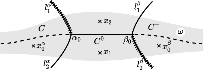
Figure 3. Stokes lines near a simple turning point.

As in §2.3, we have to consider branch cuts; we choose one on the Stokes line $l_{1}^{\alpha}$ and one on $l_{2}^{\beta}$. Assuming that $\Re z(x)$ increases towards $\alpha$ in $\omega_{\rm left}^{\alpha}$, we define exact WKB solutions as follows.

$${\bf u}_{0}^{\alpha}(x,\epsilon) ={\bf u}^{+}(x,\lambda,\epsilon,\alpha,x_{0}^{\alpha}),\quad{\bf u}_{0}^{\beta}(x,\epsilon)={\bf u}^{-}(x,\lambda,\epsilon,\beta,x_{0}^{\beta})$$

$${\bf u}_{1}^{\alpha}(x,\epsilon) ={\bf u}^{-}(x,\lambda,\epsilon,\alpha,x_{1}),\quad{\bf u}_{1}^{\beta}(x,\epsilon)={\bf u}^{-}(x,\lambda,\epsilon,\beta,x_{1})$$

$${\bf u}_{2}^{\alpha}(x,\epsilon) ={\bf u}^{+}(x,\lambda,\epsilon,\alpha,x_{2}),\quad{\bf u}_{2}^{\beta}(x,\epsilon)={\bf u}^{+}(x,\lambda,\epsilon,\beta,x_{2})$$

Remark that all these exact WKB solutions are chosen so that their asymptotic expansions in Theorem 2.14 (ii) are valid near the designated turning points. In particular, ${\bf u}_{0}^{\alpha}(x,\epsilon)$ is a decaying solution along $C^{-}(\lambda_{0})$ and ${\bf u}_{0}^{\beta}(x,\epsilon)$ is a decaying solution along $C^{+}(\lambda_{0})$. This implies the following lemma.

Lemma 2.17.

For any $\lambda_{0}$ on the asymptotic spectral arcs, there exists a complex neighbourhood $U=U(\lambda_{0})$ of $\lambda_{0}$ such that a $\lambda\in U$ is an eigenvalue of $\mathfrak{D}_{\epsilon}$ if and only if ${\bf u}_{0}^{\alpha}(x,\epsilon)$ and ${\bf u}_{0}^{\beta}(x,\epsilon)$ are linearly dependent.

Applying Proposition 2.15 near $\alpha$ and $\beta$, we have

$${\mathcal{W}}[{\bf u}_{1}^{\alpha},{\bf u}_{2}^{\alpha}]{\bf u}_{0}^{\alpha}+{\mathcal{W}}[{\bf u}_{2}^{\alpha},{\bf u}_{0}^{\alpha}]{\bf u}_{1}^{\alpha}+{\mathcal{W}}[{\bf u}_{0}^{\alpha},{\bf u}_{1}^{\alpha}]{\bf u}_{2}^{\alpha}=0,$$ (2.35)

$${\mathcal{W}}[{\bf u}_{1}^{\beta},{\bf u}_{2}^{\beta}]{\bf u}_{0}^{\beta}+{\mathcal{W}}[{\bf u}_{2}^{\beta},{\bf u}_{0}^{\beta}]{\bf u}_{1}^{\beta}+{\mathcal{W}}[{\bf u}_{0}^{\beta},{\bf u}_{1}^{\beta}]{\bf u}_{2}^{\beta}=0.$$ (2.36)

On the other hand, there is an obvious relation between ${\bf u}_{j}^{\alpha}$ and ${\bf u}_{j}^{\beta}$ for $j=1,2$:

$${\bf u}_{1}^{\beta}=e^{z(\beta,\lambda,\alpha)/\epsilon}{\bf u}_{1}^{\alpha},\quad{\bf u}_{2}^{\beta}=e^{-z(\beta,\lambda,\alpha)/\epsilon}{\bf u}_{2}^{\alpha}$$ (2.37)

where $z(\beta,\lambda,\alpha)$ is the action integral between $\alpha$ and $\beta$

$$z(\beta,\lambda,\alpha)=i\int_{\gamma(\alpha\rightsquigarrow\beta)}\sqrt{-V_{0}(t,\lambda)}dt.$$ (2.38)

It follows that ${\bf u}_{0}^{\alpha}(x,\epsilon)$ and ${\bf u}_{0}^{\beta}(x,\epsilon)$ are linearly dependent if and only if

$${\mathcal{W}}[{\bf u}_{2}^{\alpha},u_{0}^{\alpha}]{\mathcal{W}}[{\bf u}_{0}^{\beta},{\bf u}_{1}^{\beta}]={\mathcal{W}}[{\bf u}_{0}^{\alpha},{\bf u}_{1}^{\alpha}]{\mathcal{W}}[{\bf u}_{2}^{\beta},{\bf u}_{0}^{\beta}]e^{2z(\beta,\lambda,\alpha)/\epsilon}.$$

Recall the functions $g_{\pm}(x,\lambda)=\mp[\lambda+\frac{1}{2}S^{\prime}(x)\pm iA(x)]$. For a pair of simple turning points $\alpha$, $\beta$, we define an index $\delta(\alpha,\beta)$ by

$$\delta(\alpha,\beta)=\left\{\begin{array}[]{cll}-1&\text{if}\quad g_{+}(\alpha,\lambda)=g_{+}(\beta,\lambda)=0&\text{or}\quad g_{-}(\alpha,\lambda)=g_{-}(\beta,\lambda)=0,\\ 1&\text{if}\quad g_{+}(\alpha,\lambda)=g_{-}(\beta,\lambda)=0&\text{or}\quad g_{-}(\alpha,\lambda)=g_{+}(\beta,\lambda)=0.\end{array}\right.$$ (2.39)

Hence we arrive at the following result.

Theorem 2.18.

For any $\lambda_{0}$ on the asymptotic spectral arcs satisfying condition (H1), there exists a complex neighborhood $U$ of $\lambda_{0}$ such that $\lambda\in U$ is an eigenvalue of $\mathfrak{D}_{\epsilon}$ if and only if

$$m(\epsilon)e^{2z(\beta,\lambda,\alpha)/\epsilon}=1,\quad\text{with }m(\epsilon)=\frac{{\mathcal{W}}[{\bf u}_{0}^{\alpha},{\bf u}_{1}^{\alpha}]{\mathcal{W}}[{\bf u}_{2}^{\beta},{\bf u}_{0}^{\beta}]}{{\mathcal{W}}[{\bf u}_{2}^{\alpha},{\bf u}_{0}^{\alpha}]{\mathcal{W}}[{\bf u}_{0}^{\beta},{\bf u}_{1}^{\beta}]}.$$

As $\epsilon\downarrow 0$, $m(\epsilon)$ has the asymptotic behavior

$$m(\epsilon)=\delta(\alpha_{0},\beta_{0})+{\mathcal{O}}(\epsilon).$$

Proof.

It remains to check the asymptotic part of the statement. We already know from Proposition 2.16 that as $\epsilon\downarrow 0$

$${\mathcal{W}}[{\bf u}_{2}^{\alpha},{\bf u}_{0}^{\alpha}]=\mp 2+{\mathcal{O}}(\epsilon),\quad{\mathcal{W}}[{\bf u}_{0}^{\alpha},{\bf u}_{1}^{\alpha}]=2i+{\mathcal{O}}(\epsilon)$$ (2.40)

when $\alpha$ is a zero of $g_{\pm}$. Similarly, as $\epsilon\downarrow 0$ we have

$${\mathcal{W}}[{\bf u}_{2}^{\beta},{\bf u}_{0}^{\beta}]=2i+{\mathcal{O}}(\epsilon),\quad{\mathcal{W}}[{\bf u}_{0}^{\beta},{\bf u}_{1}^{\beta}]=\mp 2+{\mathcal{O}}(\epsilon)$$ (2.41)

when $\beta$ is a zero of $g_{\pm}$. These asymptotic formulas immediately give the assertion. ∎

Remark 2.19.

(The situation at the endpoints $\lambda_{D}^{(j)},j=1,2$ of the branches) It is clear from the proof that the statement of Theorem 2.18 is still valid for $\lambda_{0}$ at a limit point of the asymptotic spectral arcs where $x_{+}(\lambda_{0})$ and $x_{-}(\lambda_{0})$ coalesce to a double turning point.

2.5. What happens near the bifurcation point

Now let us suppose that $\lambda_{0}$ lies on the asymptotic spectral arcs with admissible contour $C(\lambda_{0})=C^{-}(\lambda_{0})\cup C^{0}(\lambda_{0})\cup C^{+}(\lambda_{0})$ and that the Stokes line $C^{0}(\lambda_{0})$ connecting the two simple turning points $\alpha_{0}=\alpha(\lambda_{0})$ and $\beta_{0}=\beta(\lambda_{0})$ now also contains a third simple turning point between of them, namely $\gamma_{0}=\gamma(\lambda_{0})$; of course, $\alpha,\beta$ and $\gamma$ are analytic functions defined in a neighborhood of $\lambda_{0}$.

Hence, $C^{0}(\lambda)$ consists of a Stokes line $l_{0}^{\alpha}$ connecting $\alpha$ and $\gamma$ and a Stokes line $l_{0}^{\beta}$ connecting $\beta$ and $\gamma$: $C^{0}(\lambda)=l_{0}^{\alpha}\cup l_{0}^{\beta}$. We suppose that the third Stokes line from $\gamma$ divides the region $\omega_{\rm down}^{\alpha,\beta}$ (defined as in section 2.4) into two subregions $\omega_{\rm down}^{\alpha,\gamma}$ and $\omega_{\rm down}^{\beta,\gamma}$, and take a point $x_{1}^{\alpha}$ in $\omega_{\rm down}^{\alpha,\gamma}$ and $x_{1}^{\beta}$ in $\omega_{\rm down}^{\beta,\gamma}$ (see Figure 4).

Figure 4. Stokes lines near a bifurcation point.

Now we let $\lambda$ vary in a small neighborhood of $\lambda_{0}$. Then the Stokes lines in $\omega$ change the geometric configuration. We denote by $l_{j}^{\alpha}(\lambda)$, $l_{j}^{\beta}(\lambda)$ for $j=0,1,2$ and $l^{\gamma}(\lambda)$, $l_{\alpha}^{\gamma}(\lambda)$, $l_{\beta}^{\gamma}(\lambda)$ the three Stokes lines emanating from $\alpha(\lambda)$, $\beta(\lambda)$ and $\gamma(\lambda)$ respectively such that $l_{0}^{\alpha}(\lambda_{0})=l_{\alpha}^{\gamma}(\lambda_{0})$, $l_{0}^{\beta}(\lambda_{0})=l_{\beta}^{\gamma}(\lambda_{0})$. The variation of Stokes geometry as $\lambda$ turns around $\lambda_{0}$ is illustrated in Figure 5. Remark that the Stokes lines stay close to those for $\lambda=\lambda_{0}$ by continuity.

Figure 5. Variation of the Stokes geometry around a bifurcation point.

We put branch cuts along the Stokes lines $l_{1}^{\alpha}(\lambda)$, $l_{1}^{\beta}(\lambda)$ and $l^{\gamma}(\lambda)$ (we emphasize at this point that our selection for the branch cut placed on a Stokes line emerging from $\beta$ in this case is different from the previous case where we dealt with only two turning points), and suppose that $\Re z(x)$ increases towards $\alpha$ in $\omega_{\rm left}^{\alpha}$. We define as before

$${\bf u}_{0}^{\alpha}(x,\epsilon) ={\bf u}^{+}(x,\lambda,\epsilon,\alpha,x_{0}^{\alpha}),\quad{\bf u}_{0}^{\beta}(x,\epsilon)={\bf u}^{+}(x,\lambda,\epsilon,\beta,x_{0}^{\beta})$$

$${\bf u}_{1}^{\alpha}(x,\epsilon) ={\bf u}^{-}(x,\lambda,\epsilon,\alpha,x_{1}^{\alpha}),\quad{\bf u}_{1}^{\beta}(x,\epsilon)={\bf u}^{-}(x,\lambda,\epsilon,\beta,x_{1}^{\beta})$$

$${\bf u}_{2}^{\alpha}(x,\epsilon) ={\bf u}^{+}(x,\lambda,\epsilon,\alpha,x_{2}),\quad{\bf u}_{2}^{\beta}(x,\epsilon)={\bf u}^{+}(x,\lambda,\epsilon,\beta,x_{2})$$

$${\bf u}_{1}^{\gamma,\alpha}(x,\epsilon) ={\bf u}^{-}(x,\lambda,\epsilon,\gamma,x_{1}^{\alpha})$$

$${\bf u}_{1}^{\gamma,\beta}(x,\epsilon) ={\bf u}^{-}(x,\lambda,\epsilon,\gamma,x_{1}^{\beta})$$

$${\bf u}_{2}^{\gamma}(x,\epsilon) ={\bf u}^{+}(x,\lambda,\epsilon,\gamma,x_{2})$$

For each one of the triples $\{{\bf u}_{0}^{\alpha},{\bf u}_{1}^{\alpha},{\bf u}_{2}^{\alpha}\}$, $\{{\bf u}_{2}^{\gamma},{\bf u}_{1}^{\gamma,\alpha},{\bf u}_{1}^{\gamma,\beta}\}$ and $\{{\bf u}_{0}^{\beta},{\bf u}_{1}^{\beta},{\bf u}_{2}^{\beta}\}$, we have the following relations

$${\mathcal{W}}[{\bf u}_{1}^{\alpha},{\bf u}_{2}^{\alpha}]{\bf u}_{0}^{\alpha}+{\mathcal{W}}[{\bf u}_{2}^{\alpha},{\bf u}_{0}^{\alpha}]{\bf u}_{1}^{\alpha}+{\mathcal{W}}[{\bf u}_{0}^{\alpha},{\bf u}_{1}^{\alpha}]{\bf u}_{2}^{\alpha}=0,$$ (2.42)

$${\mathcal{W}}[{\bf u}_{1}^{\gamma,\alpha},{\bf u}_{1}^{\gamma,\beta}]{\bf u}_{2}^{\gamma}+{\mathcal{W}}[{\bf u}_{1}^{\gamma,\beta},{\bf u}_{2}^{\gamma}]{\bf u}_{1}^{\gamma,\alpha}+{\mathcal{W}}[{\bf u}_{2}^{\gamma},{\bf u}_{1}^{\gamma,\alpha}]{\bf u}_{1}^{\gamma,\beta}=0,$$ (2.43)

$${\mathcal{W}}[{\bf u}_{1}^{\beta},{\bf u}_{2}^{\beta}]{\bf u}_{0}^{\beta}+{\mathcal{W}}[{\bf u}_{2}^{\beta},{\bf u}_{0}^{\beta}]{\bf u}_{1}^{\beta}+{\mathcal{W}}[{\bf u}_{0}^{\beta},{\bf u}_{1}^{\beta}]{\bf u}_{2}^{\beta}=0.$$ (2.44)

Using the obvious relations

$${\bf u}_{1}^{\beta}=e^{z(\beta,\lambda,\gamma)/\epsilon}{\bf u}_{1}^{\gamma,\beta},\quad{\bf u}_{1}^{\gamma,\alpha}=e^{z(\gamma,\lambda,\alpha)/\epsilon}{\bf u}_{1}^{\alpha}$$

$${\bf u}_{2}^{\beta}=e^{-z(\beta,\lambda,\gamma)/\epsilon}{\bf u}_{2}^{\gamma},\quad{\bf u}_{2}^{\gamma}=e^{-z(\gamma,\lambda,\alpha)/\epsilon}{\bf u}_{2}^{\alpha}$$

and

$$z(\beta,\lambda,\gamma)+z(\gamma,\lambda,\alpha)=z(\beta,\lambda,\alpha)$$

we deduce that the sum

$${\mathcal{W}}[{\bf u}_{2}^{\beta},{\bf u}_{0}^{\beta}]{\bf u}_{1}^{\beta}+{\mathcal{W}}[{\bf u}_{0}^{\beta},{\bf u}_{1}^{\beta}]{\bf u}_{2}^{\beta}$$

of the second and the third terms of (2.44) is

$${\mathcal{W}}[{\bf u}_{2}^{\beta},{\bf u}_{0}^{\beta}]e^{z(\beta,\lambda,\gamma)/\epsilon}{\bf u}_{1}^{\gamma,\beta}+{\mathcal{W}}[{\bf u}_{0}^{\beta},{\bf u}_{1}^{\beta}]e^{-z(\beta,\lambda,\gamma)/\epsilon}{\bf u}_{2}^{\gamma}$$

and this is equal to

$${\mathcal{W}}[{\bf u}_{0}^{\beta},{\bf u}_{1}^{\beta}]e^{-z(\beta,\lambda,\alpha)/\epsilon}{\bf u}_{2}^{\alpha}-\frac{{\mathcal{W}}[{\bf u}_{2}^{\beta},{\bf u}_{0}^{\beta}]}{{\mathcal{W}}[{\bf u}_{2}^{\gamma},{\bf u}_{1}^{\gamma,\alpha}]}e^{z(\beta,\lambda,\gamma)/\epsilon}\left({\mathcal{W}}[{\bf u}_{1}^{\gamma,\alpha},{\bf u}_{1}^{\gamma,\beta}]{\bf u}_{2}^{\gamma}+{\mathcal{W}}[{\bf u}_{1}^{\gamma,\beta},{\bf u}_{2}^{\gamma}]{\bf u}_{1}^{\gamma,\alpha}\right)$$

or

$${\mathcal{W}}[{\bf u}_{0}^{\beta},{\bf u}_{1}^{\beta}]e^{-z(\beta,\lambda,\alpha)/\epsilon}{\bf u}_{2}^{\alpha}\\ \qquad-\frac{{\mathcal{W}}[{\bf u}_{2}^{\beta},{\bf u}_{0}^{\beta}]}{{\mathcal{W}}[{\bf u}_{2}^{\gamma},{\bf u}_{1}^{\gamma,\alpha}]}e^{z(\beta,\lambda,\gamma)/\epsilon}\left({\mathcal{W}}[{\bf u}_{1}^{\gamma,\alpha},{\bf u}_{1}^{\gamma,\beta}]e^{-z(\gamma,\lambda,\alpha)/\epsilon}{\bf u}_{2}^{\alpha}+{\mathcal{W}}[{\bf u}_{1}^{\gamma,\beta},{\bf u}_{2}^{\gamma}]e^{z(\gamma,\lambda,\alpha)/\epsilon}{\bf u}_{1}^{\alpha}\right).$$

After some calculations, the coefficient of ${\bf u}_{2}^{\alpha}$ in this last expression is

$${\mathcal{W}}[{\bf u}_{0}^{\beta},{\bf u}_{1}^{\beta}]e^{-z(\beta,\lambda,\alpha)/\epsilon}-\frac{{\mathcal{W}}[{\bf u}_{2}^{\beta},{\bf u}_{0}^{\beta}]{\mathcal{W}}[{\bf u}_{1}^{\gamma,\alpha},{\bf u}_{1}^{\gamma,\beta}]}{{\mathcal{W}}[{\bf u}_{2}^{\gamma},{\bf u}_{1}^{\gamma,\alpha}]}e^{(z(\beta,\lambda,\gamma)-z(\gamma,\lambda,\alpha))/\epsilon}$$

while the coefficient of ${\bf u}_{1}^{\alpha}$ is

$$-\frac{{\mathcal{W}}[{\bf u}_{2}^{\beta},{\bf u}_{0}^{\beta}]{\mathcal{W}}[{\bf u}_{1}^{\gamma,\beta},{\bf u}_{2}^{\gamma}]}{{\mathcal{W}}[{\bf u}_{2}^{\gamma},{\bf u}_{1}^{\gamma,\alpha}]}e^{z(\beta,\lambda,\alpha)/\epsilon}.$$

Comparing this with (2.42), we obtain the following theorem.

Theorem 2.20.

Let $\lambda_{0}$ be a point on the asymptotic spectral arcs such that $C^{0}(\lambda_{0})$ consists of two Stokes lines; one from $\alpha_{0}$ to $\gamma_{0}$ and another one from $\beta_{0}$ to $\gamma_{0}$ (for a simple turning point $\gamma_{0}$; cf. Figure 4). There exists a neighborhood $U$ of $\lambda_{0}$ such that $\lambda\in U$ is an eigenvalue of $\mathfrak{D}_{\epsilon}$ if and only if the following condition holds

$$m_{\alpha}(\epsilon)e^{2z(\gamma,\lambda,\alpha)/\epsilon}+m_{\beta}(\epsilon)e^{2z(\gamma,\lambda,\beta)/\epsilon}=1.$$ (2.45)

Here the functions $m_{\alpha}(\epsilon)$ and $m_{\beta}(\epsilon)$ are given by

$$m_{\alpha}(\epsilon)=\frac{{\mathcal{W}}[{\bf u}_{0}^{\alpha},{\bf u}_{1}^{\alpha}]{\mathcal{W}}[{\bf u}_{1}^{\gamma,\beta},{\bf u}_{2}^{\gamma}]}{{\mathcal{W}}[{\bf u}_{2}^{\alpha},{\bf u}_{0}^{\alpha}]{\mathcal{W}}[{\bf u}_{1}^{\gamma,\alpha},{\bf u}_{1}^{\gamma,\beta}]},\quad m_{\beta}(\epsilon)=\frac{{\mathcal{W}}[{\bf u}_{0}^{\beta},{\bf u}_{1}^{\beta}]{\mathcal{W}}[{\bf u}_{2}^{\gamma},{\bf u}_{1}^{\gamma,\alpha}]}{{\mathcal{W}}[{\bf u}_{2}^{\beta},{\bf u}_{0}^{\beta}]{\mathcal{W}}[{\bf u}_{1}^{\gamma,\alpha},{\bf u}_{1}^{\gamma,\beta}]}$$

and as $\epsilon\downarrow 0$, they behave like

$$m_{\alpha}(\epsilon)=\mp 1+{\mathcal{O}}(\epsilon),\quad m_{\beta}(\epsilon)=\mp 1+{\mathcal{O}}(\epsilon)$$

where the minus/plus sign for $m_{\alpha}(\epsilon)$ [resp. $m_{\beta}(\epsilon)$] corresponds to the case where $\alpha$ (resp. $\beta$) and $\gamma$ are zeros of the same/different $g_{+}$, $g_{-}$.

Proof.

For the second part, we have in fact modulo ${\mathcal{O}}(\epsilon)$,

$${\mathcal{W}}[{\bf u}_{0}^{\alpha},{\bf u}_{1}^{\alpha}]=2i,\quad{\mathcal{W}}[{\bf u}_{0}^{\beta},{\bf u}_{1}^{\beta}]=2i,\quad{\mathcal{W}}[{\bf u}_{2}^{\gamma},{\bf u}_{1}^{\gamma,\alpha}]=2i,\quad{\mathcal{W}}[{\bf u}_{2}^{\gamma},{\bf u}_{1}^{\gamma,\beta}]=2i,$$

$${\mathcal{W}}[{\bf u}_{2}^{\alpha},{\bf u}_{0}^{\alpha}]=\mp 2,\quad{\mathcal{W}}[{\bf u}_{2}^{\beta},{\bf u}_{0}^{\beta}]=\pm 2,\quad{\mathcal{W}}[{\bf u}_{1}^{\gamma,\alpha},{\bf u}_{1}^{\gamma,\beta}]=\pm 2,$$

where the upper (resp. lower) sign corresponds to the case where the indicated turning point is a zero of $g_{+}$ (resp. $g_{-}$). ∎

Let us investigate the quantization condition (2.45) for $\lambda$ close to (but different from) $\lambda_{0}$. First, consider the actions

$$z_{\alpha}(\lambda) =z(\gamma(\lambda),\lambda,\alpha(\lambda))$$

$$z_{\beta}(\lambda) =z(\gamma(\lambda),\lambda,\beta(\lambda)).$$

The configurations from I to VI of the Stokes lines in Figure 5 correspond to $\lambda$ satisfying the following conditions on the actions $z_{\alpha}$, $z_{\beta}$:

I:

$\Re z_{\alpha}(\lambda)=\Re z_{\beta}(\lambda)<0$,

II:

$\Re z_{\beta}(\lambda)<0=\Re z_{\alpha}(\lambda)$,

III:

$\Re z_{\beta}(\lambda)=0<\Re z_{\alpha}(\lambda)$,

IV:

$\Re z_{\alpha}(\lambda)=\Re z_{\beta}(\lambda)>0$,

V:

$\Re z_{\alpha}(\lambda)=0<\Re z_{\beta}(\lambda)$,

VI:

$\Re z_{\alpha}(\lambda)<0=\Re z_{\beta}(\lambda)$,

Each condition defines a curve in the $\lambda$-plane starting from $\lambda_{0}$ (see Figure 6). For $\lambda$ not on any these curves, there is no connection between any two turning points, and such $\lambda$ cannot be o(1)-close to an eigenvalue for small enough $\epsilon$.

Figure 6. Real part of the actions $z_{\alpha}=z(\gamma,\lambda,\alpha)$ and $z_{\beta}=z(\gamma,\lambda,\beta)$

Consider first conditions I, III or V. In fact, the right hand side of the quantization condition (2.45) is exponentially small in case I and exponentially large in cases III and V, and the quantization condition cannot hold for such $\lambda$’s.

Finally, in the cases II, IV and VI, the quantization condition (2.45) reduces to the usual one of Bohr-Sommerfeld type. We have

$$\tilde{m}_{\alpha}(\epsilon)e^{2z(\gamma,\lambda,\alpha)/\epsilon}=1\quad\text{in case II},$$ (2.46)

$$\tilde{m}_{\beta}(\epsilon)e^{2z(\gamma,\lambda,\beta)/\epsilon}=1\quad\text{in case VI},$$ (2.47)

$$\tilde{m}_{\gamma}(\epsilon)e^{2z(\beta,\lambda,\alpha)/\epsilon}=1\quad\text{in case IV},$$ (2.48)

where, as $\epsilon\downarrow 0$,

$$\tilde{m}_{\alpha}(\epsilon)=\frac{m_{\alpha}(\epsilon)}{1-m_{\beta}(\epsilon)e^{2z(\gamma,\lambda,\beta)/\epsilon}}=\delta(\alpha,\gamma)+{\mathcal{O}}(\epsilon),$$ (2.49)

$$\tilde{m}_{\beta}(\epsilon)=\frac{m_{\beta}(\epsilon)}{1-m_{\alpha}(\epsilon)e^{2z(\gamma,\lambda,\alpha)/\epsilon}}=\delta(\beta,\gamma)+{\mathcal{O}}(\epsilon),$$ (2.50)

$$\tilde{m}_{\gamma}(\epsilon)=-\frac{m_{\alpha}(\epsilon)}{m_{\beta}(\epsilon)-e^{2z(\gamma,\lambda,\beta)/\epsilon}}=\delta(\alpha,\beta)+{\mathcal{O}}(\epsilon).$$ (2.51)

Notice that the above asymptotics holds a long as the absolute values of the actions $z(\gamma,\lambda,\beta)$ in (2.49), $z(\gamma,\lambda,\alpha)$ in (2.50), $z(\gamma,\lambda,\beta)$ in (2.51) are larger than $c\epsilon\log(1/\epsilon)$ for some positive constant $c$, which means $|\lambda-\lambda_{0}|\geq c^{\prime}\epsilon\log(1/\epsilon)$.

2.6. The Stokes geometry and quantization in a particular case

In this paragraph, we present the geometric configuration of the very particular case of [22]

$$A(x)=S(x)=\sech(2x),\quad x\in\mathbb{R}.$$ (2.52)

Actually, there is nothing really special about this example; it just happens that it was the first case studied numerically by Bronski in [1] and subsequently by Miller in [22].

We begin with the turning points (see Definition 2.3) of our problem. For fixed $\lambda\in\mathbb{C}$, these are the zeros (in the complex $x$-plane) of [cf. (2.1)]

$$-V_{0}(x,\lambda)=[\lambda-\tanh(2x)\sech(2x)]^{2}+\sech^{2}(2x).$$

In the present case the potential $V_{0}(\cdot,\lambda)$ is periodic with fundamental period $i\pi$. For this reason, we define the fundamental strip

$$\mathcal{S}=\{x\in\mathbb{C}|-\tfrac{\pi}{2}<\Im x\leq\tfrac{\pi}{2}\}$$ (2.53)

of the complex $x$-plane and restrict our attention only to what happens in $\mathcal{S}$. For all $\lambda\in\mathbb{C}$, the potential $V_{0}(\cdot,\lambda)$ has in $\mathcal{S}$ two fourth order $x$-poles located at $x=\pm i\pi/4$. On the other hand, the zeros of $V_{0}(\cdot,\lambda)$ are $\lambda$-dependent; there are precisely eight in $\mathcal{S}$ (counting multiplicity).

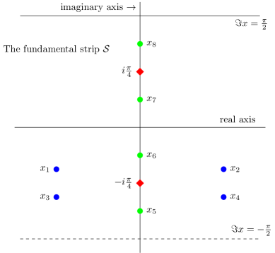
Figure 7. A (qualitative) picture showing the turning point position with blue & green circles (in the fundamental strip $\mathcal{S}$ on the $x$-complex plane) for a purely imaginary $\lambda$ ($=0.2i$). The red diamonds denote the poles of the potential.

When $\lambda$ is purely imaginary we have eight distinct (and therefore simple) zeros in $\mathcal{S}$. There are four $x$-zeros that lie on the imaginary axis, two between the poles and two outside. The remaining four $x$-zeros (in the fundamental strip) make up the vertices of a rectangle. We label the turning points in $\mathcal{S}$ as follows (the whole configuration is depicted in Figure 7).

1. The vertices of the rectangle

   • $x_{1}(\lambda)$ is the turning point with negative real part and the greatest imaginary part.

   • $x_{2}(\lambda)=-x_{1}^{*}(\lambda)$.

   • $x_{3}(\lambda)$ is the turning point with the same real part to $x_{1}(\lambda)$ and the smallest imaginary part.

   • $x_{4}(\lambda)=-x_{3}^{*}(\lambda)$.

2. The four purely imaginary turning points are labeled in order of increasing imaginary part. More precisely

   • The turning point between $-i\pi/2$ and $-i\pi/4$ is $x_{5}(\lambda)$.

   • Between $-i\pi/4$ and $0$ lies $x_{6}(\lambda)$.

   • $x_{7}(\lambda)$ is to be found between $0$ and $i\frac{\pi}{4}$.

   • Finally, the turning point between $i\pi/4$ and $i\pi/2$ is $x_{8}(\lambda)$.

In Figure 7 we show the general qualitative picture which appears in the actual numerics. The “indexing” process above provides us with an unambiguous way for the labeling of the eight turning points $x_{j}(0.2i)$, $j=1,\dots 8$ in $\mathcal{S}$.

Remark 2.21.

Using this indexing, one can show that $x_{1}$, $x_{2}$, $x_{6}$ and $x_{8}$ are zeros of $g_{-}$ [see (2.10)] while $x_{3}$, $x_{4}$, $x_{5}$ and $x_{7}$ are zeros of $g_{+}$.

For $\lambda$ not purely imaginary, the nice symmetry of the complex turning points breaks down. The turning points for non-imaginary values of $\lambda$ can be uniquely defined by analytically continuing the turning points $x_{j}(0.2i)$, $j=1,\dots 8$ along the L-shaped path (see Figure 8) from $0.2i$ to $\Re\lambda+0.2i$ (horizontally) and from $\Re\lambda+0.2i$ to $\lambda$ (vertically).

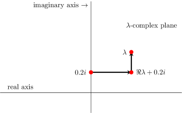
Figure 8. The L-shaped analytic continuation in the $\lambda$-complex plane of the turning points $x_{j}(0.2i)$, $j=1,\dots 8$ for a non-purely imaginary $\lambda$.

For some $\lambda\in{\mathbb{C}}$, $V_{0}(\cdot,\lambda)$ has double zeros which can be found by simply solving (with respect to $x$) simultaneously the equations $V_{0}(x,\lambda)=\tfrac{d}{dx}V_{0}(x,\lambda)=0$. It is useful to compute these double zeros since it turns out that they are related to the end-points of the (semiclassical) asymptotic spectrum. One easily sees that these double zeros are present only for four values of $\lambda$, namely

$$\lambda_{D}=i\sigma\sqrt{\frac{1}{2}+\frac{1+i\tau\sqrt{7}}{8}}\Bigg{(}1-\frac{1+i\tau\sqrt{7}}{4}\Bigg{)}\quad\text{where}\quad\sigma,\tau=\pm 1$$ (2.54)

and are given by the solutions of the transcendental equations

$$\tanh(2x)=\frac{1+i\tau\sqrt{7}}{4i\sigma}\quad\text{where}\quad\sigma,\tau=\pm 1$$

We adopt the notation $\lambda_{D}^{(j)}$, $j=1,\dots,4$, by requiring that the point $\lambda_{D}^{(j)}$ is located in the $j^{\rm th}$ quadrant in the complex $\lambda$-plane. Observe that the set of the four $\lambda_{D}$’s in (2.54) can be written as $(\lambda,-\lambda,\lambda^{*},-\lambda^{*})$. These four $\lambda_{D}$’s turn out to be -as we shall eventually discover numerically- the endpoints of the four branches of a ${{\mathrel{\begin{subarray}{c}\Ydown\\[-2.87996pt] \Yup\end{subarray}}}}$-shaped asymptotic spectrum in the complex $\lambda$-plane, symmetric to both of the coordinate axes. The Y-shaped set consisting of the points in the upper half-plane $\mathbb{H}^{+}$ is the union of three arcs which intersect at a point $i\mu_{\otimes}$ (the numerical experiments in [22] indicate that $\mu_{\otimes}\approx 0.28$).

We now proceed to investigate for which $\lambda\in{\mathbb{C}}$ there exists an admissible contour (as defined in paragraph §2). For these values of $\lambda$ the WKB analysis for locating the eigenvalues will be possible. For each $j,k=1,\dots,8$ with $j\neq k$, we now define the complex-valued action integrals

$$I_{jk}(\lambda)=z(x_{k}(\lambda),\lambda,x_{j}(\lambda))=i\int_{C^{0}(x_{j}(\lambda)\rightsquigarrow x_{k}(\lambda))}\sqrt{-V_{0}(t,\lambda)}dt.$$ (2.55)

We construct well-defined branches for these functions by defining signs of the square root for $\lambda=0.2i$ and applying analytic continuation along the same L-shaped path as was used to define the turning points $x_{j}(\lambda)$, $j=1,\dots,8$ (again refer to Figure 8). For reasons that will be explained later, we restrict our attention only to $I_{12}$, $I_{16}$ and $I_{26}$.

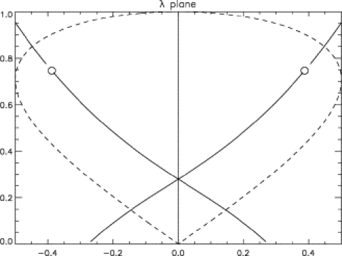
Figure 9. Candidates for the asymptotic spectral arcs on the $\lambda$-upper-half-plane. The dashed curve in this figure (which is Fig. 3 in [22]) is the so called real-turning-point curve (it is the set $\{\,\lambda\in\mathbb{C}\mid\exists\hskip 2.0ptr\in\mathbb{R}\hskip 2.0pt:\hskip 2.0ptV_{0}(r,\lambda)=0\,\}$); it plays no role in our analysis.

We confine ourselves to the upper $\lambda$-half-plane, since the spectrum of the Dirac operator in (2.1) is symmetric with respect to the real axis. The three conditions $\Re[I_{12}(\lambda)]=0$, $\Re[I_{16}(\lambda)]=0$ and $\Re[I_{26}(\lambda)]=0$ [recall (2.13)] yield three curves in the upper $\lambda$-half-plane (see Figure 9). We label them as follows

$$\Lambda_{12} =\{\,\lambda\in\mathbb{H}^{+}\mid\Re[I_{12}(\lambda)]=0\,\},$$

$$\Lambda_{16} =\{\,\lambda\in\mathbb{H}^{+}\mid\Re[I_{16}(\lambda)]=0\,\},$$

$$\Lambda_{26} =\{\,\lambda\in\mathbb{H}^{+}\mid\Re[I_{26}(\lambda)]=0\,\}.$$

Actually, the curve $\Lambda_{12}$ coincides with the upper imaginary semi-axis while the curves $\Lambda_{16}$ and $\Lambda_{26}$ have negative and positive slopes respectively. There is only one point of intersection in the upper $\lambda$-half-plane, which lies on the imaginary axis and is denoted by $\lambda_{\otimes}=i\mu_{\otimes}$. It is easily observed that $\lambda_{D}^{(1)}$ belongs to the curve $\Lambda_{26}$ while $\lambda_{D}^{(2)}=-\lambda_{D}^{(1)\hskip 2.0pt*}$ belongs to the curve $\Lambda_{16}$.

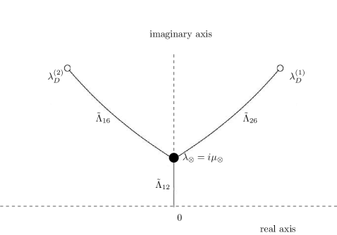
Figure 10. The asymptotic spectral arcs on the $\lambda$-plane.

Our understanding is that [22] only considers $I_{12}$, $I_{16}$ and $I_{26}$ because the curves described by the rest of the equations $\Re[I_{jk}(\lambda)]=0$ (as well as curves in the $\lambda$-plane arising from equations corresponding to pairs of turning points in different period strips) play no new role in the WKB analysis of the particular potentials (2.52). More precisely, even though Stokes curves connecting the respective turning points exist, there are no progressive paths connecting to $\pm\infty$. For similar reasons one eventually eliminates portions of the curves $\Lambda_{12}$, $\Lambda_{16}$ and $\Lambda_{26}$. Specifically, we only consider (see Figure 10)

• $\tilde{\Lambda}_{12}$, the part of ${\Lambda}_{12}$ that lies between $0$ and $\lambda_{\otimes}$, endpoints included

• $\tilde{\Lambda}_{26}$, which lies between $\lambda_{\otimes}$ and $\lambda_{D}^{(1)}$, endpoints included

• $\tilde{\Lambda}_{16}$, which lies between $\lambda_{\otimes}$ and $\lambda_{D}^{(2)}$, endpoints included.

These are the asymptotic spectral arcs defined in Definition 2.9, in our specific case (2.52). The union of these three arcs defines a Y-shaped set in the upper $\lambda$-half-plane which is the part of the asymptotic spectrum that lies on the upper-half-plane. It has been numerically observed in [22] that the semiclassical spectrum observed by Bronski in [1] coincides with this asymptotic spectrum computed here!

We must point out however, that we have a different argument why there are no eigenvalues away from this union of asymptotic spectral arcs. The numerics of [22] show that for $\lambda$ away from this union of asymptotic spectral arcs there is always a progressive path from $-\infty$ to $+\infty$ which coincides with the real axis for large $|x|$. From standard WKB theory these $\lambda$’s cannot be eigenvalues .

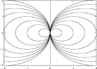
Figure 11. The behavior of Stokes lines near a pole in $x$-plane. This is Fig. 5 in [22].

We now examine carefully the geometry of the solutions of the differential equation (2.12) in the complex $x$-plane. From each simple turning point $x_{j}(\lambda)$ three orbits of (2.12) are emerging at angles of $2\pi/3$ (on the other hand there is an infinite number of orbits meeting at each forth-order pole; see Figure 11). These are Stokes curves of (2.12).

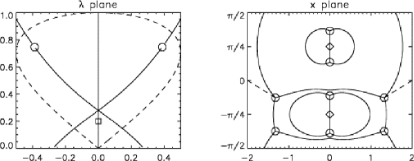
Figure 12. On the left, the $\lambda$-plane with a small square indicating point $\lambda=0.2i\in\tilde{\Lambda}_{12}$, below the bifurcation point. On the right, for that particular of $\lambda$, the fundamental strip $\mathcal{S}$ in the $x$-plane, showing clearly the Stokes lines that emanate from all turning points. This is Fig. 4 in [22].

For $\lambda=0.2i\in\tilde{\Lambda}_{12}$ (located below $\lambda_{\otimes}$ on the imaginary axis), the corresponding situation of the $x$-plane is shown in Figure 12. We observe that there is a Stokes line $C^{0}$ connecting $x_{1}(0.2i)$ and $x_{2}(0.2i)$. Furthermore, there exist progressive paths $C^{-}$, $C^{+}$ joining $x_{1}(0.2i)$ to $-\infty$ and $x_{2}(0.2i)$ to $+\infty$ respectively .

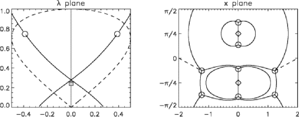
Figure 13. On the left, the $\lambda$-plane, with a small square indicating a point just below close the bifurcation point $\lambda_{\otimes}\approx 0.28i$. On the right, for that particular value of $\lambda$, the strip $\mathcal{S}$ of the $x$-plane and the Stokes lines in $\mathcal{S}$ that emanate from all turning points. Compare with case IV of Figure 5. This is Fig. 6 in [22].

For a value of $\lambda$ on the imaginary axis coming very close to the triple intersection point $\lambda_{\otimes}$ (but still imaginary and just below $\lambda_{\otimes}$), the situation on the $x$-plane still looks similar to that we already examined (cf. Figure 13). The complex turning point $x_{6}(\lambda)$ is moving up very close to the Stokes line that continues to connect $x_{1}(\lambda)$ and $x_{2}(\lambda)$. This proximity becomes more evident as $\lambda$ approaches the triple intersection point $\lambda_{\otimes}$. The progressive paths emerging from $x_{1}(\lambda)$, $x_{2}(\lambda)$ continue to exist.

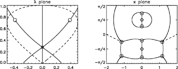
Figure 14. On the left, the $\lambda$-plane in the extreme case when $\lambda$ is right at the bifurcation point $\lambda_{\otimes}$. On the right, the $x$-plane with the Stokes lines in $\mathcal{S}$. Compare with Figure 4 or the central picture of Figure 5. This is Fig. 7 in [22].

When $\lambda=\lambda_{\otimes}$ (see Figure 14) there is no Stokes line connecting $x_{1}(\lambda_{\otimes})$ and $x_{2}(\lambda_{\otimes})$ without passing through another turning point. Parts of the two paths previously connecting $x_{6}(\lambda_{\otimes})$ to $x_{5}(\lambda_{\otimes})$ have now partly coalesced with the path connecting $x_{1}(\lambda_{\otimes})$ and $x_{2}(\lambda_{\otimes})$. Hence $x_{1}(\lambda_{\otimes})$ and $x_{2}(\lambda_{\otimes})$ are now connected to $x_{6}(\lambda_{\otimes})$ via Stokes lines. But the remaining Stokes line from $x_{6}(\lambda_{\otimes})$ continues to pass through the pole at $-i\pi/4$. The three conditions $\Re[I_{12}(\lambda_{\otimes})]=0$, $\Re[I_{26}(\lambda_{\otimes})]=0$, $\Re[I_{16}(\lambda_{\otimes})]=0$ are satisfied simultaneously and the corresponding Stokes lines meet at $x_{6}(\lambda_{\otimes})$ and at a $2\pi/3$ angle from each other. For this special value of $\lambda$, there is a connected sequence of two Stokes lines and the progressive paths continue to exist.

Figure 15. Progressive paths (dashed curves) in the $x$-plane when $\lambda$ is slightly off the asymptotic spectrum; cf. Figure 5, cases I, III, V.

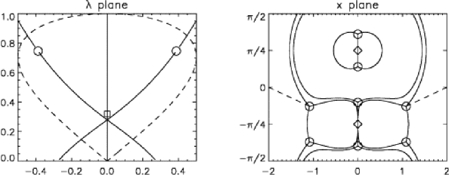
Figure 16. The $\lambda$-plane on the left, for a specific $\lambda\in\Lambda_{12}$ just above the bifurcation point $\lambda_{\otimes}$. On the right, the $x$-plane with the Stokes lines in $\mathcal{S}$. Compare with case I of Figure 5. Note that one can draw a progressive path from $-\infty$ to $+\infty$ which passes above $x_{1}$, just below $x_{6}$ and above $x_{2}$ (see Figure 15, top). Hence there is no eigenvalue semiclassically. This is Fig. 8 in [22].

Having completed the description of what happens when $\lambda\in\tilde{\Lambda}_{12}$, there are five more remaining directions in the complex $\lambda$-plane all meeting at the triple intersection point $\lambda_{\otimes}$ (cf. Figure 10).

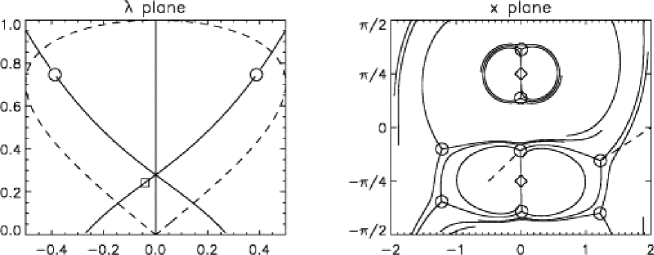
Figure 17. The $\lambda$-plane on the left, for a particular $\lambda\in\Lambda_{26}$ just below $\lambda_{\otimes}\approx 0.28i$. On the right, the $x$-plane with the Stokes lines in $\mathcal{S}$. Compare with case III of Figure 5. Note that one can draw a progressive path from $-\infty$ to $+\infty$ which passes below $x_{1}$, just above $x_{6}$ and above $x_{2}$ (see Figure 15, bottom left). Hence there is no eigenvalue semiclassically. This is Fig. 9 in [22].

Now suppose we continue along the imaginary axis above $\lambda_{\otimes}$ (see Figure 16). There is no more admissible connection between the turning points $x_{1}(\lambda)$, $x_{2}(\lambda)$. There are paths emanating from $x_{1}(\lambda)$, $x_{2}(\lambda)$ (see Definition 2.7) meeting at the double pole of $\sqrt{-V_{0}(\cdot,\lambda)}$ so the holomorphic deformation is impossible, requiring us to restrict the WKB analysis described so far only to the section $\tilde{\Lambda}_{12}$. Note the existence of a progressive path from $-\infty$ to $+\infty$ which passes above $x_{1}$, just below $x_{6}$ and above $x_{2}$ (see dashed curve at the top of Figure 15). Hence there is no eigenvalue semiclassically.

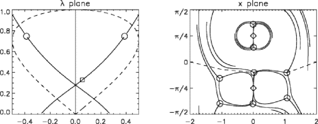
Figure 18. The $\lambda$-plane on the left, for a particular $\lambda\in\tilde{\Lambda}_{26}$ just above $\lambda_{\otimes}\approx 0.28i$. On the right, the $x$-plane with the Stokes lines in $\mathcal{S}$. Compare with case VI of Figure 5. This is Fig. 10 in [22].

Same observations for different pairs of turning points show that the WKB analysis only works for $I_{12}$, $I_{16}$ and $I_{26}$ (and indeed only for the sections $\tilde{\Lambda}_{12}$, $\tilde{\Lambda}_{26}$ and $\tilde{\Lambda}_{16}$). One can examine the rest of the cases by checking Figures 17 through 21.

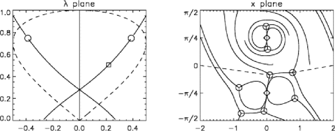
Figure 19. The $\lambda$-plane on the left, for a particular $\lambda\in\tilde{\Lambda}_{26}$ with $\Im\lambda$ greater than that shown in Figure 18 but less than $\Im\lambda_{D}^{(1)}$. On the right, the $x$-plane with the Stokes lines in $\mathcal{S}$. This is Fig. 11 in [22].

Finally we give the quantization condition of eigenvalues along $\tilde{\Lambda}_{12}$, $\tilde{\Lambda}_{26}$ and $\tilde{\Lambda}_{16}$ away from the bifurcation point $\lambda_{\otimes}$, and in a neighborhood of $\lambda_{\otimes}$ using the results of the previous subsections.

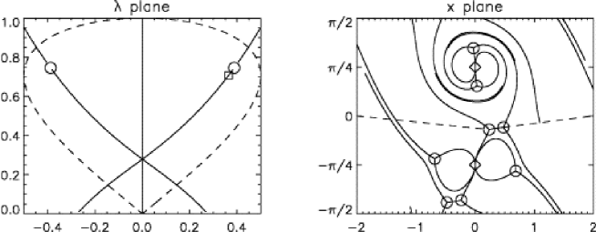
Figure 20. On the left, the $\lambda$-plane for a specific $\lambda\in\tilde{\Lambda}_{26}$ just below $\lambda_{D}^{(1)}$. On the right, the $x$-plane with the Stokes lines in $\mathcal{S}$. This is Fig. 12 in [22].

Theorem 2.22.

Let $(j,k)$ be $(1,2),(2,6)$ or $(1,6)$. For any $\epsilon$-independent $\delta>0$ and $\lambda_{0}\neq 0$ on $\tilde{\Lambda}_{jk}$, fixed and independent of $\epsilon$, satisfying $|\lambda_{0}-\lambda_{\otimes}|>\delta$, there exist a complex neighborhood $U$ of $\lambda_{0}$ and a function $m_{jk}(\epsilon)$ with a uniform asymptotic behavior $m_{jk}(\epsilon)=-1+{\mathcal{O}}(\epsilon)$ in $U$, such that $\lambda\in U$ is an eigenvalue of $\mathfrak{D}_{\epsilon}$ if and only if

$$m_{jk}(\epsilon)e^{2z(\beta,\lambda,\alpha)/\epsilon}=1.$$

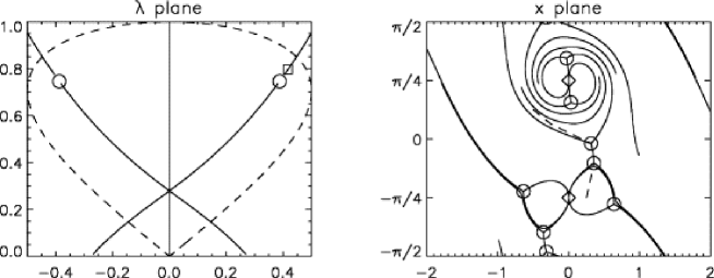
Figure 21. On the left, the $\lambda$-plane for a specific $\lambda\in\Lambda_{26}$ just above $\lambda_{D}^{(1)}$. On the right, the $x$-plane with the Stokes lines in $\mathcal{S}$. Note that one can draw a progressive path that is a deformation of the real line in such a way that it crosses the Stokes line from $x_{2}$ to $x_{6}$ transversally. Hence there is no eigenvalue semiclassically. This is Fig. 13 in [22].

Theorem 2.23.

There exists a neighborhood $U$ of $\lambda_{\otimes}$ and functions $m_{\alpha}(\epsilon)$, $m_{\beta}(\epsilon)$ with uniform asymptotic behaviors $m_{\alpha}(\epsilon)=-1+{\mathcal{O}}(\epsilon)$, $m_{\beta}(\epsilon)=-1+{\mathcal{O}}(\epsilon)$ in $U$, such that $\lambda\in U$ is an eigenvalue of $\mathfrak{D}_{\epsilon}$ if and only if

$$m_{\alpha}(\epsilon)e^{2z(\gamma,\lambda,\alpha)/\epsilon}+m_{\beta}(\epsilon)e^{2z(\gamma,\lambda,\beta)/\epsilon}=1.$$ (2.56)

Remark 2.24.

We claim that no eigenvalue can appear away from the asymptotic spectral arcs. Although we do not present a rigorous proof of this fact, it follows from the numerical investigation of the geometry of turning points and Stokes lines for different values of $\lambda$. For example, Figure 16, Figure 17 and Figure 21 show that for $\lambda$ slightly off the asymptotic spectral arcs, a progressive path from $x=-\infty$ to $x=+\infty$ does exist, which is in fact real near $x=\pm\infty$. It follows easily from standard WKB theory that such $\lambda$ cannot be eigenvalues. Indeed, in view of part (ii) of Theorem 2.14, and the fact that $S$ is real near $x=\pm\infty$, the important factor in formula (2.25) for ${\bf u}^{+}$ that determines the behavior at $x=\pm\infty$, is the exponential $\exp(z/\epsilon)$. If $\Re z$ is monotonic along a path from $-\infty$ to $+\infty$ then it is impossible that the solution decays at both ends.

Remark 2.25.

The question arises whether there is a possibility of a general proof of the fact that no eigenvalue can appear away from the asymptotic spectral arcs. A consequence of this would be a general proof that the limiting spectrum (the minimal set such that every actual eigenvalue lies $\epsilon$-close to this set) would be what we have called the asymptotic spectrum (which we defined in terms of the existence of an admissible path). In turn that would prove that the limiting spectrum is a union of analytic arcs.

A possible strategy is suggested by an analogous problem appearing in the semiclassical analysis of the inverse scattering problem in [19] where a crucial ingredient of the proof is the existence of appropriate steepest descent paths. The existence proof in [20] requires the study of an associated max-min variational problem.

In our own problem here, we can define a generalized admissible contour as a contour that is either admissible in the sense of Definition 2.13 (extended to allow for double turning points as degenerate cases) or a progressive path from $x=-\infty$ to $x=+\infty$. The inequalities defining progressiveness and the equations defining Stokes lines can be interpreted as variational Euler-Lagrange conditions for a max-min problem. We expect that a proof along the lines of [20] will show the existence of the desired contour which is either a progressive path from $x=-\infty$ to $x=+\infty$ (hence no eigenvalue) or an admissible contour in the sense of Definition 2.13 (hence an asymptotic spectral arc).

3. Eigenvalues That Lie Near Zero

Note: In this section $A(x)=S(x)=\sech(2x)$ for simplicity. But the theory applies very generally.

3.1. Preparations

We now turn our attention to the semiclassical behavior of eigenvalues (and their corresponding norming constants) of the Zakharov-Shabat operator that lie near zero. We will focus on a neighborhood $\mathscr{D}$ of the real axis (to be appropriately specified later on) and start with the problem

$$\mathfrak{D}_{\epsilon}\mathbf{u}(x)=\lambda\mathbf{u}(x),\quad x\in\mathscr{D}$$

where

• the Dirac (or Zakharov-Shabat) operator is defined by

  $$\mathfrak{D}_{\epsilon}=\begin{bmatrix}-\frac{\epsilon}{i}\frac{d}{dx}&-iA(x)\exp\{iA(x)/\epsilon\}\\ -iA(x)\exp\{-iA(x)/\epsilon\}&\frac{\epsilon}{i}\frac{d}{dx}\end{bmatrix}$$

• $\epsilon>0$ is the semiclassical parameter,

• $\mathbf{u}=[u_{1}\hskip 3.0ptu_{2}]^{T}$ is a function from $\mathscr{D}$ to $\mathbb{C}^{2}$ and

• $\lambda\in{\mathbb{C}}$ represents the spectral parameter.

First, we apply the change of variables [cf. equation (4) in [22]]

$$w_{\pm}=\frac{u_{2}\exp\{iA/(2\epsilon)\}\pm u_{1}\exp\{-iA/(2\epsilon)\}}{\sqrt{A\pm i(\lambda+A^{\prime}/2)}}.$$ (3.1)

Then for the lower sign (minus), the equation reads

$$w_{-}^{\prime\prime}=\Bigg{[}-\epsilon^{-2}\Big{\{}A(x)^{2}+[\lambda+\tfrac{A^{\prime}(x)}{2}]^{2}\Big{\}}\\ +\frac{3}{4}\bigg{\{}\frac{A^{\prime}(x)-i\frac{A^{\prime\prime}(x)}{2}}{A(x)-i[\lambda+\tfrac{A^{\prime}(x)}{2}]}\bigg{\}}^{2}-\frac{1}{2}\frac{A^{\prime\prime}(x)-i\frac{A^{\prime\prime\prime}(x)}{2}}{A(x)-i[\lambda+\tfrac{A^{\prime}(x)}{2}]}\Bigg{]}w_{-}$$ (3.2)

where we dropped the dependence of $w_{-}$ on $(x,\lambda,\epsilon)$ for notational simplicity and let prime denote differentiation with respect to $x$. Hence, dropping the subscript, and considering only the upper half $\lambda$-plane due to symmetry, we are led to the following proposition.

Proposition 3.1.

Finding the discrete spectrum of $\mathfrak{D}_{\epsilon}$ is equivalent to finding the values of $\lambda\in\mathbb{H}^{+}$ for which equation

$$\frac{d^{2}w}{dx^{2}}=[\epsilon^{-2}V_{0}(x,\lambda)+g(x,\lambda)]w$$ (3.3)

has an $L^{2}(\mathscr{D})$ solution. In this equation, the leading order potential $V_{0}(x,\lambda)$ satisfies

$$V_{0}(x,\lambda)=-\Big{\{}A(x)^{2}+[\lambda+\tfrac{A^{\prime}(x)}{2}]^{2}\Big{\}}$$ (3.4)

while the correction $g(x,\lambda)$ is given by

$$g(x,\lambda)=\frac{3}{4}\bigg{\{}\frac{A^{\prime}(x)-i\frac{A^{\prime\prime}(x)}{2}}{A(x)-i[\lambda+\tfrac{A^{\prime}(x)}{2}]}\bigg{\}}^{2}-\frac{1}{2}\frac{A^{\prime\prime}(x)-i\frac{A^{\prime\prime\prime}(x)}{2}}{A(x)-i[\lambda+\tfrac{A^{\prime}(x)}{2}]}.$$ (3.5)

In this section, we are only interested in the behavior of the eigenvalues that lie near zero. So, let us first fix some set $\mathscr{O}$ on the spectral plane that satisfies the following condition.

(H2):

The set $\mathscr{O}$ is an open and simply connected set, proper subset of ${\mathcal{R}}_{0}\cap\mathbb{H}^{+}$ [recall the formula for the mumerical range (2.4) and of course here $S(x)=A(x)=\sech(2x)$] and located in such a way that its intersection with $\tilde{\Lambda}_{12}$ (see Figure 10) is a single interval and has no common points with either $\tilde{\Lambda}_{16}$ or $\tilde{\Lambda}_{26}$.

From now on, we shall only consider eigenvalues $\lambda$ that lie in a set $\mathscr{O}$ satisfying (H2).

3.2. Solutions in a neighborhood of only one simple turning point

In this subsection we shall confine the study of the differential equation (3.3) to some domain in which it has only one simple turning point. Let us be more precise.

Assumption 3.2.

For $\epsilon>0$, consider the differential equation

$$\frac{d^{2}w}{dx^{2}}=[\epsilon^{-2}V_{0}(x,\lambda)+g(x,\lambda)]w,\quad(x,\lambda)\in\mathscr{D}\times\mathscr{O}$$

where $V_{0}(x,\lambda)$ is given by (3.4) and $g(x,\lambda)$ by (3.5) for $A(x)=\sech(2x)$. We assume that the following hold true.

• We denote by $c=c(\lambda)$, one of the following (simple) turning points: $x_{1}$, $x_{2}$, $x_{6}$ or $x_{8}$ (cf. §2.6) which are (simple) zeros of $g_{-}$ [see (2.10), recalling that $V_{0}=g_{-}g_{+}$].

• The set $\mathscr{D}\subset{\mathbb{C}}$ (in the $x$-plane) is an open and simply connected neighborhood of the real axis so that $c$ is an interior point and the only transition point (of the equation) in it.

• The set $\mathscr{O}$ satisfies condition $\mathbf{(H2})$.

Remark 3.3.

Clearly, we can always choose $\mathscr{D}$ and $\mathscr{O}$ so that the assumption above holds.

Remark 3.4.

From the assumptions above, it follows that

• the function $(x-c)^{-1}V_{0}(x,\lambda)$ is holomorphic and non-vanishing throughout $\mathscr{D}$ (including $c$).

• the function $g(x,\lambda)$ is holomorphic in $\mathscr{D}$.

Having placed the assumptions on our equation, we continue as follows. We introduce a new variable $\zeta=\zeta(\cdot,\lambda):\mathscr{D}\rightarrow{\mathbb{C}}$ defined by

$$\zeta=\bigg{(}\int_{\gamma(c\rightsquigarrow x)}V_{0}^{1/2}(t,\lambda)dt\bigg{)}^{2/3}.$$ (3.6)

In order to choose the branch, we proceed as follows. We expand $(t-c)^{-1}V_{0}(t,\lambda)$ in a Taylor-series in the neighborhood of $c$, namely

$$(t-c)^{-1}V_{0}(t,\lambda)=f_{0}+f_{1}(t-c)+f_{2}(t-c)^{2}+\dots$$

for a sequence $\{f_{n}\}_{n\in{\mathbb{N}}_{0}}$ of complex numbers (depending on $\lambda$) where $f_{0}\neq 0$. Substituting for $V_{0}$ in (3.6) and integrating term by term, we find that $\zeta$ has a Taylor-series expansion (in the neighborhood of $c$) that begins with

$$\zeta=\Big{(}\frac{2}{3}\Big{)}^{2/3}f_{0}^{1/3}(x-c)\Big{[}1+\frac{1}{5}\frac{f_{1}}{f_{0}}(x-c)+\dots\Big{]}$$ (3.7)

We select any branch of the coefficient $f_{0}^{1/3}$ that is convenient to us, and this fixes the relation between $\zeta$ and $x$ in the neighborhood of $c$; elsewhere, $\zeta$ is defined by continuity.

Next, we define $\Delta=\zeta(\mathscr{D},\lambda)$. We suppose that $\mathscr{D}$ is restricted in such a way that the mapping $\zeta(\cdot,\lambda):\mathscr{D}\rightarrow\Delta$ is one-to-one [it is already onto; of course this implies that $c$ is the only point in $\mathscr{D}$ at which $\zeta(\cdot,\lambda)$ vanishes]. Hence, it follows that $\zeta(\cdot,\lambda)\in\mathscr{H}(\mathscr{D})$ and therefore the $\zeta(\cdot,\lambda)$-mapping from $\mathscr{D}$ on to $\Delta$ is conformal. Also, we define the following.

Definition 3.5.

Let $x(\cdot,\lambda)$ be the inverse of $\zeta(\cdot,\lambda)$ and $S_{j}$, $j=0,1,2$ be the sectors defined by

$$(2j-1)\frac{\pi}{3}\leq\mathrm{ph}\zeta\leq(2j+1)\frac{\pi}{3}.$$

The sets

$$\mathscr{D}_{j}=x(\Delta\cap S_{j},\lambda),\quad\text{for}\quad j=0,1,2$$

shall be called the principal regions associated with the transition point $c$.

Furthermore, we define

$$\hat{f}(x,\lambda)\equiv\frac{4}{9}\frac{V_{0}(x,\lambda)}{\zeta(x,\lambda)}=\Big{[}\frac{d\zeta}{dx}(x,\lambda)\Big{]}^{2}$$ (3.8)

where it is clear that $\hat{f}(\cdot,\lambda)$ is holomorphic and non-vanishing in $\mathscr{D}$. Subsequently, we introduce the notion of a balancing function.

Definition 3.6.

Consider a function $\Omega(t)$ which is any conveniently chosen positive function of the complex variable $t$ that is continuous and satisfies the asymptotics

$$\Omega(t)=\mathcal{O}(t^{1/2})\quad\text{uniformly in the neighborhood of}\quad t=\infty.$$

Such a function shall be called a balancing function, and for $j,k=0,1,2$ with $j\neq k$ we set

$$\rho_{j,k}=\sup_{t\in S_{j}\cup S_{k}}\{\Omega(t)\mathsf{M}_{j,k}^{2}(t)\}$$ (3.9)

where the $\mathsf{M}_{j,k}$ are the auxiliary functions found in appendix A (they are related to the modified Bessel functions).

Remark 3.7.

Using the bounds we have for $\mathsf{M}_{j,k}(t)$, the fact that $\mathsf{M}_{j,k}(t)$ is continuous in $S_{j}\cup S_{k}$ and the asymptotics for the balancing function, it is easy to realize that the quantities $\rho_{j,k}$ are always finite.

We fix a way to measure the error of the approximation by setting an error-control function.

Definition 3.8.

We define an error-control function $H(x,\lambda,\epsilon)$ of equation (3.3) to be any primitive of

$$\frac{1}{\Omega(\epsilon^{-2/3}\zeta)}\bigg{\{}\frac{1}{\hat{f}^{1/4}(x,\lambda)}\frac{d^{2}}{dx^{2}}\Big{[}\frac{1}{\hat{f}^{1/4}(x,\lambda)}\Big{]}-\frac{g(x,\lambda)}{\hat{f}^{1/2}(x,\lambda)}\bigg{\}}$$

where for $\hat{f}^{1/4}$ and $\hat{f}^{1/2}$ we choose any continuous branches in $\mathscr{D}$ such that $\hat{f}^{1/2}=(\hat{f}^{1/4})^{2}$. Using (3.8) and $V_{0}$ instead of $\hat{f}$ the above becomes

$$\frac{3}{2}\frac{\zeta^{1/2}}{\Omega(\epsilon^{-2/3}\zeta)}\bigg{\{}\frac{1}{V_{0}^{1/4}(x,\lambda)}\frac{d^{2}}{dx^{2}}\Big{[}\frac{1}{V_{0}^{1/4}(x,\lambda)}\Big{]}-\frac{g(x,\lambda)}{V_{0}^{1/2}(x,\lambda)}\bigg{\}}-\frac{5}{16}\frac{1}{\zeta^{2}\Omega(\epsilon^{-2/3}\zeta)}.$$

Finally, before stating the theorem about the solutions of (3.3), let us fix some complementary notation.

Definition 3.9.

Take two points $x_{j}\in\textsf{clos}(\mathscr{D}_{j})$ and $y_{k}\in\textsf{clos}(\mathscr{D}_{k})$ where $j,k\in\{0,1,2\}$. A path $\mathscr{P}:\gamma(x_{j}\rightsquigarrow y_{k})$ [meaning a Jordan arc comprising of a finite chain of $R_{2}$ arcs; where an $R_{2}$ arc is an arc $\sigma=\sigma(s)$ ($s$ being the arc parameter) such that $\sigma^{\prime\prime}(s)$ is continuous and $\sigma^{\prime}(s)$ does not vanish], shall be called a progressive path joining $x_{j},y_{k}$ if it satisfies the following “monotonicity condition”: as $x$ travels along $\mathscr{P}$ from $x_{j}$ to $y_{k}$, the function

$$\Re\int_{\gamma(x_{j}\rightsquigarrow x)}V_{0}^{1/2}(t,\lambda)dt$$ (3.10)

is non-decreasing . We choose the branch of the integral in (3.10) so that the whole function is continuous, staying non-positive in $\mathscr{D}_{j}$ while non-negative in $\mathscr{D}_{k}$. Furthermore, we define

$$\mathsf{H}_{k}(x_{j})=\{\,x\in\mathscr{D}_{j}\cup\mathscr{D}_{k}\mid\exists\hskip 3.0pt\text{a progressive path}\hskip 3.0pt\gamma(x_{j}\rightsquigarrow x)\subset\mathscr{D}_{j}\cup\mathscr{D}_{k}\,\}.$$

Definition 3.10.

Let $\mathscr{P}:\gamma(a\rightsquigarrow b)$ be a progressive path between the points $a$ and $b$. We define the variation of the error-control function $H$ along $\mathscr{P}$ to be

$$\mathcal{V}_{\mathscr{P}}[H](\lambda,\epsilon)\equiv\mathcal{V}_{a,b}[H](\lambda,\epsilon)\\ =\int_{\gamma(a\rightsquigarrow b)}\bigg{|}\frac{1}{\Omega(\epsilon^{-2/3}\zeta)}\bigg{\{}\frac{1}{\hat{f}^{1/4}(t,\lambda)}\frac{d^{2}}{dt^{2}}\Big{[}\frac{1}{\hat{f}^{1/4}(t,\lambda)}\Big{]}-\frac{g(t,\lambda)}{\hat{f}^{1/2}(t,\lambda)}\bigg{\}}\bigg{|}dt.$$

All these, lead us to the next important theorem about the solutions to equation (3.3).

Theorem 3.11.

Consider Assumption 3.2, let $a,b\in{\mathbb{C}}$ be arbitrary and choose a reference point $a_{j}\in\textsf{clos}(\mathscr{D}_{j})$, $j=0,1,2$ (the reference point could be $\infty$). Also, for $k\in\{0,1,2\}$ such that $k\neq j$, consider the set $\mathsf{H}_{k}(a_{j})$ of points in $\mathscr{D}_{j}\cup\mathscr{D}_{k}$ that can be joined to $a_{j}$ with a progressive path $\mathscr{P}$ in $\mathscr{D}_{j}\cup\mathscr{D}_{k}$ [with the understanding that if $\zeta(a_{j})$ is at infinity, then we suppose that it is the point at infinity on a path $P$ in $S_{j}$ and require $\zeta(\mathscr{P})$ to coincide with $P$ in a neighborhood of $\zeta(a_{j})$]. Then for every $\epsilon>0$, equation (3.3), namely

$$\frac{d^{2}w}{dx^{2}}=[\epsilon^{-2}V_{0}(x,\lambda)+g(x,\lambda)]w$$

with $V_{0},g$ given by (3.4) and (3.5) respectively, has a solution $w(x,\lambda,\epsilon)$ (depending of course on $a,b$ and $a_{j}$) that is holomorphic in $\mathscr{D}\setminus\{c\}$ and continuous at $c$. Furthermore, when $x\in\mathsf{H}_{k}(a_{j})$ we have

$$w(x,\lambda,\epsilon)=\hat{f}^{-1/4}(x,\lambda)\big{[}aU_{j}(\epsilon^{-2/3}\zeta)+bU_{k}(\epsilon^{-2/3}\zeta)+R(\zeta,\lambda,\epsilon)\big{]}$$

where $U_{j}$, $U_{k}$ are the MBF defined in appendix A. The remainder $R$ satisfies the following precise estimates

$$\frac{|R(\zeta,\lambda,\epsilon)|}{\mathsf{M}_{j,k}(\epsilon^{-2/3}\zeta)},\frac{\Big{|}\frac{\partial R}{\partial\zeta}(\zeta,\lambda,\epsilon)\Big{|}}{\epsilon^{-2/3}\mathsf{N}_{j,k}(\epsilon^{-2/3}\zeta)},\frac{\Big{|}\frac{\partial[\zeta^{1/4}R(\zeta,\lambda,\epsilon)]}{\partial\zeta}\Big{|}}{\epsilon^{-2/3}|\zeta|^{1/4}\hat{\mathsf{N}}_{j,k}(\epsilon^{-2/3}\zeta)}\\ \leq\frac{\sigma_{j,k}}{\rho_{j,k}}\mathsf{E}_{j,k}(\epsilon^{-2/3}\zeta)\bigg{(}\exp\Big{\{}\frac{\rho_{j,k}}{3|\lambda_{j,k}|}\epsilon^{2/3}\mathcal{V}_{a_{j},x}[H](x,\lambda,\epsilon)\Big{\}}-1\bigg{)}$$ (3.11)

where the variation of $H$ is being evaluated along $\mathscr{P}$ (see Definition 3.10), the $\rho_{j,k}$ are given by (3.9) and the quantities $\sigma_{j,k},\lambda_{j,k}$ satisfy

$$\sigma_{j,k}=\sup_{p\in\zeta(\mathscr{P})}\bigg{\{}\frac{\Omega(\epsilon^{-2/3}p)\mathsf{M}_{j,k}(\epsilon^{-2/3}p)}{\mathsf{E}_{j,k}(\epsilon^{-2/3}p)}\big{|}aU_{j}(\epsilon^{-2/3}p)+bU_{k}(\epsilon^{-2/3}p)\big{|}\bigg{\}}$$ (3.12)

and

$$\lambda_{j,k}=\frac{\sin\Big{[}(k-j)\frac{\pi}{3}\Big{]}}{\sin\frac{\pi}{3}}$$ (3.13)

respectively. When $x\in\mathscr{D}_{k}$, the bounds (3.11) for the error, apply only to the branch of $w$ obtained by analytic continuation from a neighborhood of $c$ in $\mathscr{D}_{j}$ by rotation through an angle $2(k-j)\frac{\pi}{3}$.

Proof.

For the proof see §§3.3-3.6 in Olver’s [24] with $m=3$. The statement of the theorem can be found in §3.3 as Theorem 3.1. ∎

Remark 3.12.

For the theorem to be meaningful, it is necessary that the right-hand side of (3.11) is finite. Recall that $\rho_{j,k}$ are finite (cf. Remark 3.7) and that in our case $1/|\lambda_{j,k}|$ are finite as well [see (3.13) and recall that $(k-j)\neq 0\hskip 2.0pt{\rm mod}3$]. But $\mathcal{V}_{\mathscr{P}}[H]$ has to converge (the variation of $H$ is calculated along $\mathscr{P}$) and also the $\sigma_{j,k}$ have to be finite. It is seen that the quantity in brackets in (3.12) is finite at all finite points $p\in S_{j}\cup S_{k}$ and bounded as $p\rightarrow\infty$ in $S_{k}$. As $p\rightarrow\infty$ in an internal part of $S_{j}$ (see appendix A) however, the quantity in brackets is unbounded, unless $b=0$. Accordingly, if $\zeta(a_{j})=\infty$ in an internal part of $S_{j}$, then the theorem may be applied only in the case $b=0$.

Remark 3.13.

In order to deal with the behavior near the remaining (simple) turning points, namely $x_{3}$, $x_{4}$, $x_{5}$ and $x_{7}$, instead of the differential equation for $w_{-}$, we consider the differential equation for $w_{+}$ [see (3.1)] and apply exactly the same strategy like the one just presented.

3.3. Asymptotic estimates for the error terms

Let us now consider a circumstance in which the error-term $R$ is sufficiently small for the theorem to supply meaningful approximations when $\epsilon$ is small. But let us first define the function

$$F(x,\lambda)=\int\bigg{\{}\frac{1}{V_{0}^{1/4}(x,\lambda)}\frac{d^{2}}{dx^{2}}\Big{[}\frac{1}{V_{0}^{1/4}(x,\lambda)}\Big{]}-\frac{g(x,\lambda)}{V_{0}^{1/2}(x,\lambda)}\bigg{\}}dx$$ (3.14)

where for this integral we shall not use paths that intersect $c$, while for $V_{0}^{1/4},V_{0}^{1/2}$ we adopt any branches, provided they are continuous and the latter is the square of the former. With this in mind, we have the following result.

Theorem 3.14.

Let Assumption 3.2 be satisfied (observe that $V_{0},g$ are independent of $\epsilon$), consider $a_{j},a_{k}$ to be arbitrary points in $\textsf{clos}(\mathscr{D}_{j})$ and $\textsf{clos}(\mathscr{D}_{k})$ respectively (including the point at infinity) and let $\mathscr{P}$ be a progressive path joining $a_{j}$ and $a_{k}$. Then as $\epsilon\downarrow 0$, we have

$$\mathcal{V}_{\mathscr{P}}[H](\lambda,\epsilon)=\mathcal{O}(\epsilon^{1/3}).$$

Proof.

Referring to Theorem 4.1(ii) when $m=3$ in [24], one only needs to check that

• the function $1/\zeta(x)$ [refer to (3.6)] and

• the function $F(x,\lambda)$ in (3.14)

are of bounded variation as $x\rightarrow a_{j}$ or $a_{k}$ along $\mathscr{P}$. ∎

3.4. The connection theorem

In this section, we will state a theorem that concerns the connection of solutions of our equation between two principal regions near a turning point. But first, we reformulate the geometric concepts introduced in §3.2 using a new variable $\xi_{c}$, in order to avoid referring explicitly to the variable $\zeta$. We begin with a definition (see Definition 2.6).

Definition 3.15.

The curves in the complex $x$-plane having the equation

$$\Re\int_{\gamma(c\rightsquigarrow x)}V_{0}^{1/2}(t,\lambda)dt=0$$

are called the Stokes curves associated with the turning point $c$ . Either branch may be used for the square root of $V_{0}$, provided continuity is maintained.

Since $c$ is a simple turning point of equation (3.3), there are three distinct Stokes curves intersecting at $c$ at an angle of $2\pi/3$. All of them occupy the same Riemann sheet. Using the conformality of the mapping one can prove that: (i) a Stokes curve can either terminate at $c$ or at a boundary point of $\mathscr{D}$, and (ii) that no Stokes curve intersects itself or any other Stokes curve on the same Riemann sheet (except c).

Evidently, the Stokes curves are boundaries of principal regions (each principal region includes its bounding Stokes curves). From here on, we suppose that in each principal region there is a one-to-one relation between $x$ and any continuous branch of the integral $\int V_{0}^{1/2}(t,\lambda)dt$ (which is equivalent to the fact that the mapping from $\mathscr{D}$ to $\Delta$ is one-to-one).

We start by fixing an arbitrarily chosen principal region and name it $\mathscr{D}_{0}$. We then define $\mathscr{D}_{1}$ to be the successive principal domain encountered as we pass around $c$ in a counterclockwise direction and similarly set $\mathscr{D}_{2}$ be the successive principal region (to $\mathscr{D}_{0}$) encountered as we pass around $c$ in a clockwise direction. Whatever choice we make for $\mathscr{D}_{0}$, the labeling can be made consistent with that chosen before, by appropriately choosing the branch of $f_{0}^{1/3}$ in (3.7).

Definition 3.16.

Take $j\in\{0,1,2\}$. We shall refer to $\mathscr{D}_{j}\cap\mathscr{D}_{(j+1)\hskip 2.0pt{\rm mod}3}$ as the left boundary of $\mathscr{D}_{j}$. Also we will call $\mathscr{D}_{j}\cap\mathscr{D}_{(j-1)\hskip 2.0pt{\rm mod}3}$, the right boundary of $\mathscr{D}_{j}$.

Next, in each principal region $\mathscr{D}_{j}$, $j\in\{0,1,2\}$ associated with $c$ we define

$$\xi_{c}(x,\lambda)=\int_{\gamma(c\rightsquigarrow x)}V_{0}^{1/2}(t,\lambda)dt$$ (3.15)

taking the branch that is continuous with $\Re\xi_{c}(x,\lambda)\geq 0$. This determines a function of $x$ that is continuous in $\mathscr{D}$ except on the Stokes curves. Fix a $j\in\{0,1,2\}$. Clearly, for $x$ on the left boundary of $\mathscr{D}_{j}$ we have $\xi_{c}(x,\lambda)\in i{\mathbb{R}}^{+}$, while on the right boundary of $\mathscr{D}_{j}$ we have $\xi_{c}(x,\lambda)\in i{\mathbb{R}}^{-}$. Since the left boundary of $\mathscr{D}_{j}$ is also the right boundary of $\mathscr{D}_{(j+1)\hskip 2.0pt{\rm mod}3}$ and the right boundary of $\mathscr{D}_{j}$ is also the left boundary of $\mathscr{D}_{(j-1)\hskip 2.0pt{\rm mod}3}$, we realize that $\xi_{c}(x,\lambda)$ changes sign when it crosses a principal curve. Finally we redefine the notion of the progressive path (cf. Definition 3.9).

Definition 3.17.

Any Jordan arc $\mathscr{P}$ comprising of a finite chain of $R_{2}$ arcs and having the property that $\Re\xi_{c}(\cdot,\lambda)$ is monotonic on the intersection of $\mathscr{P}$ with any principal region, shall (also) be called a progressive path associated with $c$.

Before stating the main theorem of this section, let us formulate an important lemma first.

Lemma 3.18.

Consider the differential equation (3.3), taking into account Assumption 3.2. Also, let $j\in\{0,1,2\}$, pick a boundary point or point at infinity $a_{j}\in\textsf{clos}(\mathscr{D}_{j})$ and consider a progressive path $\mathscr{P}$ in $\mathscr{D}_{j}$ passing from $a_{j}$. Then equation (3.3) has a unique solution $w(x,\lambda,\epsilon)\in\mathscr{H}(\mathscr{D})$ and satisfies

$$V_{0}^{1/4}(x,\lambda)w(x,\lambda,\epsilon) \sim e^{-\xi_{c}(x,\lambda)/\epsilon}\quad\text{as}\quad x\rightarrow a_{j}\quad\text{along}\quad\mathscr{P}$$

$$\frac{\partial[V_{0}^{1/4}(x,\lambda)w(x,\lambda,\epsilon)]}{\partial x} \sim-\frac{1}{\epsilon}V_{0}^{1/2}(x,\lambda)e^{-\xi_{c}(x,\lambda)/\epsilon}\quad\text{as}\quad x\rightarrow a_{j}\quad\text{along}\quad\mathscr{P}.$$

Proof.

Using Theorem 11.1 in chapter 6 of Olver’s book [25] one needs to realize that

• $\Re\xi_{c}(x,\lambda)\rightarrow+\infty$ as $x\rightarrow a_{j}$ along $\mathscr{P}$ and

• $\mathcal{V}_{a_{j},x}[F]$ converges as $x\rightarrow a_{j}$ along $\mathscr{P}$.

It follows that such a solution exists, is holomorphic and additionally satisfies the desired asymptotics. Since $\Re\xi_{c}(x,\lambda)\rightarrow+\infty$ as $x\rightarrow a_{j}$ along $\mathscr{P}$, this solution is recessive and hence unique. ∎

We are now ready for current section’s main theorem.

Theorem 3.19.

Consider the differential equation (3.3), taking into account Assumption 3.2. Also, let $j,k\in\{0,1,2\}$ with $k\neq j$, pick two boundary points or points at infinity, namely $a_{j}\in\textsf{clos}(\mathscr{D}_{j})$, $a_{k}\in\textsf{clos}(\mathscr{D}_{k})$ (different from $c$) and consider a progressive path $\mathscr{P}$ in $\mathscr{D}_{j}\cup\mathscr{D}_{k}$ joining them. Then the unique solution $w(x,\lambda,\epsilon)$ of equation (3.3) provided by the previous lemma, satifies the following asymptotics as $x\rightarrow a_{k}$ along $\mathscr{P}$

$$V_{0}^{1/4}(x,\lambda)w(x,\lambda,\epsilon) \sim i^{k-j-1}(\lambda_{j,k}+\kappa_{0})e^{\xi_{c}(x,\lambda)/\epsilon}$$

$$\frac{\partial[V_{0}^{1/4}(x,\lambda)w(x,\lambda,\epsilon)]}{\partial x} \sim\frac{i^{k-j-1}}{\epsilon}(\lambda_{j,k}+\kappa_{0})V_{0}^{1/2}(x,\lambda)e^{\xi_{c}(x,\lambda)/\epsilon}$$

where $\kappa_{0}$ is independent of $x$ and subject to the bound

$$|\kappa_{0}|\leq(1+\lambda_{j,k}^{2})^{1/2}\bigg{(}\exp\Big{\{}\frac{\rho_{j,k}}{3|\lambda_{j,k}|}\epsilon^{2/3}\mathcal{V}_{\mathscr{P}}[H]\Big{\}}-1\bigg{)}.$$

Proof.

The proof of this theorem follows from Theorem 5.1 in [24] merely by checking that

• $\Re\xi_{c}(x,\lambda)\rightarrow+\infty$ as $x\rightarrow a_{j}$ along $\mathscr{P}$,

• $\mathcal{V}_{a_{j},x}[F]$ converges as $x\rightarrow a_{j}$ along $\mathscr{P}$ and

• $\Re\xi_{c}(x,\lambda)\rightarrow+\infty$ as $x\rightarrow a_{k}$ along $\mathscr{P}$.

∎

3.5. The asymptotic form of the connection theorem

In this section, we construct asymptotic estimates for the error-terms in Theorem 3.19 for small $\epsilon>0$ by applying the results from §3.3. Let us first fix some notation that will be used in this and the following sections. We have

• We use the notation “$\doteq$” to state that besides the validity of the equation shown, the corresponding equation obtained by formally differentiating with respect to $x$, ignoring the differentiation of the $\mathcal{O}$-terms present, also stands true.

• When an $\mathcal{O}$-term appears in an equation it is understood to hold uniformly for all the values of $x$ associated with that equation.

• With $\chi(\epsilon)$, we denote any positive function of $\epsilon$ such that as $\epsilon\downarrow 0$ it satisfies

  $$\chi(\epsilon)\rightarrow 0\quad\text{and}\quad 1/\chi(\epsilon)=\mathcal{O}(\epsilon^{-1}).$$ (3.16)

• Lastly, let $a,b$ be two points on a path $\mathscr{P}$. We write $[a,b]_{\mathscr{P}}$, $(a,b)_{\mathscr{P}}$, $[a,b)_{\mathscr{P}}$ and $(a,b]_{\mathscr{P}}$ to denote the part of $\mathscr{P}$ that lies between $a$ and $b$, with endpoints included or not, accordingly.

With these in mind, we formulate the following theorem.

Theorem 3.20.

For $\epsilon>0$, consider the differential equation

$$\frac{d^{2}w}{dx^{2}}=[\epsilon^{-2}V_{0}(x,\lambda)+g(x,\lambda)]w,\quad(x,\lambda)\in\mathscr{D}\times\mathscr{O}$$ (3.17)

and assume Assumption 3.2. Also, let $j,k\in\{0,1,2\}$ with $k\neq j$ and consider a progressive path $\mathscr{P}$ in $\mathscr{D}_{j}\cup\mathscr{D}_{k}$. Pick points $a_{j},b_{j},b_{k},a_{k}$, in that order on $\mathscr{P}$, neither of which depends on $\epsilon$ nor coincides with $c$, and such that $a_{j}\in\textsf{clos}(\mathscr{D}_{j})$, $a_{k}\in\textsf{clos}(\mathscr{D}_{k})$, $b_{j}\in\mathscr{D}_{j}$ and $b_{k}\in\mathscr{D}_{k}$ [thus $a_{j},a_{k}$ (but not $b_{j},b_{k}$) may be boundary points of $\mathscr{D}$, including the point at infinity]. Finally, let the function $w(x,\lambda,\epsilon)$ denote the solution of the differential equation (3.17) (as provided by Lemma 3.18).Then, on $[b_{k},a_{k})_{\mathscr{P}}$, the analytic continuation of $w(x,\lambda,\epsilon)$ [obtained by passing from $\mathscr{D}_{j}$ to $\mathscr{D}_{k}$ in the same sense as the sign of $(k-j)$], is given by

$$\text{case A}:\quad w(x,\lambda,\epsilon) =w_{\rm I}(x,\lambda,\epsilon)\quad\text{or}$$

$$\text{case B}:\quad w(x,\lambda,\epsilon) =w_{\rm I,1}(x,\lambda,\epsilon)+w_{\rm L}(x,\lambda,\epsilon)\quad\text{or}$$

$$\text{case C}:\quad w(x,\lambda,\epsilon) =w_{\rm I,-1}(x,\lambda,\epsilon)+w_{\rm R}(x,\lambda,\epsilon)$$

depending on whether $b_{k}$ is an interior point of $\mathscr{D}_{k}$ (case A), or $[b_{k},a_{k})_{\mathscr{P}}$ lies on the left boundary of $\mathscr{D}_{k}$ (case B), or $[b_{k},a_{k})_{\mathscr{P}}$ lies on the right boundary of $\mathscr{D}_{k}$ (case C). Here, $w_{\rm I}(x,\lambda,\epsilon)$, $w_{\rm I,\pm 1}(x,\lambda,\epsilon)$, $w_{\rm L}(x,\lambda,\epsilon)$ and $w_{\rm R}(x,\lambda,\epsilon)$ are solutions of the differential equation (3.17) so that on $[b_{k},a_{k})_{\mathscr{P}}$ they have the following asymptotic forms as $\epsilon\downarrow 0$

$$\begin{rcases}V_{0}^{1/4}(x,\lambda)w_{\rm I}(x,\lambda,\epsilon)\\ V_{0}^{1/4}(x,\lambda)w_{\rm I,1}(x,\lambda,\epsilon)\\ V_{0}^{1/4}(x,\lambda)w_{\rm I,-1}(x,\lambda,\epsilon)\end{rcases}\doteq i^{k-j-1}[\lambda_{j,k}+\mathcal{O}(\hat{\chi})]e^{\xi_{c}(x,\lambda)/\epsilon}$$

$$V_{0}^{1/4}(x,\lambda)w_{\rm L}(x,\lambda,\epsilon)\doteq i^{k-j}[\lambda_{j,k+1}+\mathcal{O}(\hat{\chi})]e^{-\xi_{c}(x,\lambda)/\epsilon}$$

$$V_{0}^{1/4}(x,\lambda)w_{\rm R}(x,\lambda,\epsilon)\doteq-i^{k-j}[\lambda_{j,k-1}+\mathcal{O}(\hat{\chi})]e^{-\xi_{c}(x,\lambda)/\epsilon}.$$

In these relations, $\lambda_{j,k}$ are given by (3.13), $V_{0}^{1/4}(x,\lambda)$ denotes the branch obtained from that used in Lemma 3.18 [equivalently see (3.19) below] by analytic continuation in the same manner as for $w(x,\lambda,\epsilon)$ and the function $\hat{\chi}=\hat{\chi}(\epsilon)$ is defined by

$$\hat{\chi}(\epsilon)=\max\{\epsilon,\chi(\epsilon)\}.$$ (3.18)

Proof.

For the proof, the reader can refer to Theorem 6.1 in [24] with $m=3$ and the function $g$ analytic at $c$. It suffices to see that the following are true.

• The function $1/\xi_{c}(x,\lambda)$ [see (3.15)] is of bounded variation on $(a_{j},b_{j}]_{\mathscr{P}}$ and $[b_{k},a_{k})_{\mathscr{P}}$

• The function $F(x,\lambda)$ given by (3.14) is of bounded variation on $(a_{j},b_{j}]_{\mathscr{P}}$ and $[b_{k},a_{k})_{\mathscr{P}}$ and

• The function $w(x,\lambda,\epsilon)$ satisfies the following.

  • For $x\in(a_{j},b_{j}]_{\mathscr{P}}$

    $$V_{0}^{1/4}(x,\lambda)w(x,\lambda,\epsilon)\doteq[1+\mathcal{O}(\chi)]e^{-\xi_{c}(x,\lambda)/\epsilon}\quad\text{as}\quad\epsilon\downarrow 0$$ (3.19)

  • As $x\rightarrow a_{j}$ along $\mathscr{P}$, the functions

    $$e^{\xi_{c}(x,\lambda)/\epsilon} V_{0}^{1/4}(x,\lambda)w(x,\lambda,\epsilon),$$

    $$V_{0}^{-1/2}(x,\lambda)e^{\xi_{c}(x,\lambda)/\epsilon} \frac{\partial[V_{0}^{1/4}(x,\lambda)w(x,\lambda,\epsilon)]}{\partial x}$$

    tend to non-zero finite limits.

∎

Remark 3.21.

Even though $w_{\rm I}(x,\lambda,\epsilon)$ and $w_{\rm I,\pm 1}(x,\lambda,\epsilon)$ have the same asymptotics as $\epsilon\downarrow 0$ on $[b_{k},a_{k})_{\mathscr{P}}$, it should be emphasized that they do represent distinct solutions of equation (3.17).

3.6. Application of the connection theorem

In this section, we apply Theorem 3.20 to prove a Bohr-Sommerfeld type quantization condition for the eigenvalues that lie near zero. Once again, we begin by some geometric formulations that will pave the way to the final result.

Let now $\mathscr{D}$ denote a simply connected open neighborhood of the real axis that contains only two simple turning points of our differential equation. Let us be more precise and make the following assumption.

Assumption 3.22.

Consider the differential equation

$$\frac{d^{2}w}{dx^{2}}=[\epsilon^{-2}V_{0}(x,\lambda)+g(x,\lambda)]w,\quad(x,\lambda)\in\mathscr{D}\times\mathscr{O}$$

where

• The functions $V_{0}(x,\lambda)$ and $g(x,\lambda)$ are given by

  $$V_{0}(x,\lambda)=-\Big{\{}A(x)^{2}+[\lambda+\tfrac{A^{\prime}(x)}{2}]^{2}\Big{\}}$$

  $$g(x,\lambda)=\frac{3}{4}\bigg{\{}\frac{A^{\prime}(x)-i\frac{A^{\prime\prime}(x)}{2}}{A(x)-i[\lambda+\tfrac{A^{\prime}(x)}{2}]}\bigg{\}}^{2}-\frac{1}{2}\frac{A^{\prime\prime}(x)-i\frac{A^{\prime\prime\prime}(x)}{2}}{A(x)-i[\lambda+\tfrac{A^{\prime}(x)}{2}]}$$

  for $A(x)=\sech(2x)$.

• The set $\mathscr{O}$ is an open and simply connected set (of the $\lambda$-plane), proper subset of ${\mathcal{R}}_{0}\cap\mathbb{H}^{+}$ [see (2.4) with $S(x)=A(x)=\sech(2x)$] located in such a way that its intersection with $\tilde{\Lambda}_{12}$ is a single interval and moreover it does not have common points with either $\tilde{\Lambda}_{16}$ or $\tilde{\Lambda}_{26}$. Also, let $c\equiv x_{1}$ and $\hat{c}\equiv x_{2}$ be the two distinct simple zeros of $g_{-}$ as introduced in §2.6 [see Remark 2.21; recall that $V_{0}=g_{-}g_{+}$ where $g_{\pm}$ are given by (2.10)].

• The set $\mathscr{D}\subset{\mathbb{C}}$ is an open and simply connected domain (of the $x$-plane) so that it contains the real axis and that the only transition points of the differential equation in it, are $c$ and $\hat{c}$.

Remark 3.23.

Observe that the assumption above implies that

• the function $(x-c)^{-1}(x-\hat{c})^{-1}V_{0}(x,\lambda)$ is holomorphic and non-vanishing throughout $\mathscr{D}$ (including $c,\hat{c}$) and

• the function $g(x,\lambda)$ is holomorphic in $\mathscr{D}$.

Let the WKB approximation of a solution of our differential equation be given at a point in $\textsf{clos}(\mathscr{D})$ other than one of the turning points. Then the WKB approximation of the same solution at any other point (except at a turning point) can be found by at most two applications of Theorem 3.20.

As was done previously, we associate with the two transition points the functions

$$\xi_{c}(x,\lambda) =\int_{\gamma(c\rightsquigarrow x)}V_{0}^{1/2}(t,\lambda)dt$$

$$\xi_{\hat{c}}(x,\lambda) =\int_{\sigma(\hat{c}\rightsquigarrow x)}V_{0}^{1/2}(t,\lambda)dt.$$

For the former, namely $\xi_{c}(x,\lambda)$, we take a branch of the integral so that $\Re\xi_{c}(x,\lambda)\geq 0$ and so that it makes $\xi_{c}(x,\lambda)$ continuous except at $\Re\xi_{c}(x,\lambda)=0$. The last relation defines a set of three Stokes curves emanating from $c$. We refer to any Stokes curve emanating from the turning point $c$ as a $c$-Stokes curve . We argue similarly for $\xi_{\hat{c}}(x,\lambda)$.

On the $\xi$-plane, where

$$\xi(x,\lambda)=\int V_{0}^{1/2}(x,\lambda)dx$$

in which the integration constant is arbitrary and the branch is chosen in a continuous way, we have the following. The $c$-Stokes curves and the $\hat{c}$-Stokes curves are mapped to straight lines parallel to the imaginary axis. Conformal mapping theory shows that the $c$-Stokes curves intersect on the same Riemann sheet only at $c$ and a similar assertion holds for $\hat{c}$. Also, $c$-Stokes curves and $\hat{c}$-Stokes curves do not intersect on the same sheet. However, in our case $c$ and $\hat{c}$ are linked together by a common Stokes curve: the interval $[\xi(c),\xi(\hat{c})]$ (on the $\xi$-plane) is parallel to the imaginary axis.

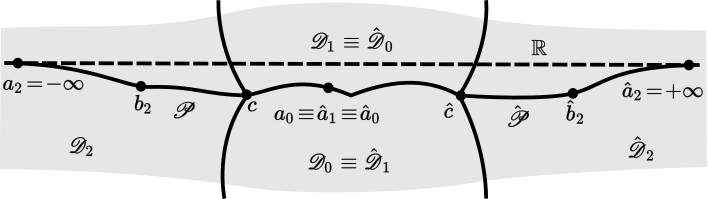
Figure 22. The configuration on the $x$-plane for the case of near-zero eigenvalues.

Now, we assemble all the results of this paragraph and formulate the theorem about the eigenvalues that lie near zero.

Theorem 3.24.

Consider Assumption 3.22. Then for any $\lambda_{0}\in\mathscr{O}$, there exists a complex neighborhood $U$ of $\lambda_{0}$ such that $\lambda\in U$ is an eigenvalue of $\mathfrak{D}_{\epsilon}$ if and only if

$$n(\lambda,\epsilon)e^{2\xi_{c}(\hat{c})/\epsilon}=1$$

where as $\epsilon\downarrow 0$, the function $n(\lambda,\epsilon)$ satisfies

$$n(\lambda,\epsilon)=-1+\mathcal{O}(\epsilon).$$

Proof.

Figure 22 shows the geometric configuration in the complex $x$-plane for our case, along with the labeling of the corresponding principal regions. In particular, there are two regions, namely $\mathscr{D}_{0}=\hat{\mathscr{D}}_{1}$ and $\mathscr{D}_{1}=\hat{\mathscr{D}}_{0}$, that have both $c$ and $\hat{c}$ on their boundaries, each being a principal region with respect to either turning point.

We would like to connect the WKB form of a solution on the segment $(-\infty,b_{2}]_{\mathscr{P}}$ of a progressive path $\mathscr{P}\in\mathscr{D}_{2}$, to the the WKB form of the same solution on the segment $[\hat{b}_{2},+\infty)_{\hat{\mathscr{P}}}$ of a progressive path $\hat{\mathscr{P}}\in\hat{\mathscr{D}}_{2}$. The essential observation for one to notice is the relation between $\xi_{c}$ and $\xi_{\hat{c}}$ in the intermediate area. We have

$$\xi_{c}(x)-\xi_{\hat{c}}(x)=\xi_{c}(\hat{c})=-\xi_{\hat{c}}(c),\quad x\in\mathscr{D}_{0}\cup\mathscr{D}_{1}.$$

We take an arbitrary point $a_{0}$ on the common Stokes curve linking $c$ and $\hat{c}$. Then, $a_{0}$ can be joined to $b_{2}$ by an extension of $\mathscr{P}$ that passes through $c$ and is progressive; now $[c,a_{0}]_{\mathscr{P}}$ coincides with the common Stokes curve. By applying Theorem 3.20 (with $k=0$ and $j=2$) we find that the WKB form of $w(x,\lambda,\epsilon)$ at $a_{0}$ is given by

$$w(x,\lambda,\epsilon)=w_{\rm I,1}^{(c)}(x,\lambda,\epsilon)+w_{\rm L}^{(c)}(x,\lambda,\epsilon)$$

where as $\epsilon\downarrow 0$ we have the asymptotics

$$V_{0}^{1/4}(x,\lambda)w_{\rm I,1}^{(c)}(x,\lambda,\epsilon) \doteq i^{-3}[\lambda_{2,0}+\mathcal{O}(\hat{\chi})]e^{\xi_{c}(x,\lambda)/\epsilon}$$

$$V_{0}^{1/4}(x,\lambda)w_{\rm L}^{(c)}(x,\lambda,\epsilon) \doteq i^{-2}[\lambda_{2,1}+\mathcal{O}(\hat{\chi})]e^{-\xi_{c}(x,\lambda)/\epsilon}.$$

where $\hat{\chi}(\epsilon)$ is given by (3.18) and (3.16).

To prepare for passage through $\hat{c}$, we observe that $\mathscr{D}_{0}=\hat{\mathscr{D}}_{1}$. Consequently, we relabel $a_{0}$ now naming it $\hat{a}_{1}$ and extend $\hat{\mathscr{P}}$, still progressive, to pass through $\hat{c}$ and continue along the common Stokes curve until $\hat{a}_{1}$ is reached. In the WKB form of $w(x,\lambda,\epsilon)$ at $\hat{a}_{1}$ found by passage through $c$, there are two terms: $w_{\rm I,1}^{(c)}(x,\lambda,\epsilon)$ and $w_{\rm L}^{(c)}(x,\lambda,\epsilon)$. Let us find how these two behave when they pass through $\hat{c}$.

The contribution from $w_{\rm L}^{(c)}(x,\lambda,\epsilon)$ to the WKB form on $[\hat{b}_{2},+\infty)_{\hat{\mathscr{P}}}$ is obtained by replacing $e^{-\xi_{c}(x,\lambda)/\epsilon}$ by $e^{-\xi_{c}(\hat{c},\lambda)/\epsilon}e^{-\xi_{\hat{c}}(x,\lambda)/\epsilon}$ and applying Theorem 3.20 (with $c$ replaced by $\hat{c}$ and $k=2,j=1$). We find

$$w_{\rm L}^{(c)}(x,\lambda,\epsilon)=w_{\rm I}^{(\hat{c})}(x,\lambda,\epsilon)$$

where as $\epsilon\downarrow 0$ we have

$$V_{0}^{1/4}(x,\lambda)w_{\rm I}^{(\hat{c})}(x,\lambda,\epsilon)\doteq i^{0}[\lambda_{1,2}+\mathcal{O}(\hat{\chi})]e^{-\xi_{c}(\hat{c},\lambda)/\epsilon}e^{\xi_{\hat{c}}(x,\lambda)/\epsilon}.$$

To handle the contribution from $w_{\rm I,1}^{(c)}(x,\lambda,\epsilon)$, the key step is to regard $a_{0}$ as a member of $\hat{\mathscr{D}}_{0}$ and relabel it as $\hat{a}_{0}$. Since this entails crossing a Stokes curve, $\xi_{\hat{c}}(x,\lambda)$ is replaced by $-\xi_{\hat{c}}(x,\lambda)$. Thus, $e^{\xi_{c}(x,\lambda)/\epsilon}$ becomes $e^{\xi_{c}(\hat{c},\lambda)/\epsilon}e^{-\xi_{\hat{c}}(x,\lambda)/\epsilon}$, where $\hat{c}$ is regarded as a member of $\mathscr{D}_{0}$ in calculating $\xi_{c}(\hat{c},\lambda)\in i{\mathbb{R}}^{+}$ and $x\in\hat{\mathscr{D}}_{0}$. Now, by an application of Theorem 3.20 (with $c$ replaced by $\hat{c}$ and $k=2,j=0$), we find

$$w_{\rm I,1}^{(c)}(x,\lambda,\epsilon)=w_{\rm I}^{(\hat{c})}(x,\lambda,\epsilon)$$

where as $\epsilon\downarrow 0$, the following asymptotic form is satisfied

$$V_{0}^{1/4}(x,\lambda)w_{\rm I}^{(\hat{c})}(x,\lambda,\epsilon)\doteq-i^{2}[\lambda_{0,2}+\mathcal{O}(\hat{\chi})]e^{\xi_{c}(\hat{c},\lambda)/\epsilon}e^{\xi_{\hat{c}}(x,\lambda)/\epsilon}.$$

Now, combining the last two results, we are capable of obtaining the behavior of $w(x\lambda,\epsilon)$ on $[\hat{b}_{2},+\infty)_{\hat{\mathscr{P}}}$. As $\epsilon\downarrow 0$ we find that for $x\in[\hat{b}_{2},+\infty)_{\hat{\mathscr{P}}}$ we have

$$V_{0}^{1/4}(x,\lambda)w(x,\lambda,\epsilon)\doteq\Big{\{}[1+\mathcal{O}(\hat{\chi})]e^{-\xi_{c}(\hat{c},\lambda)/\epsilon}+[1+\mathcal{O}(\hat{\chi})]e^{\xi_{c}(\hat{c},\lambda)/\epsilon}\Big{\}}e^{\xi_{\hat{c}}(x,\lambda)/\epsilon}.$$

But $\lambda$ is an eigenvalue of $\mathfrak{D}_{\epsilon}$ if and only if $w(x,\lambda,\epsilon)$ is decaying as $x\rightarrow+\infty$ which is equivalent with the fact that the quantity inside the braces in the last result is zero. This easily leads to

$$n(\lambda,\epsilon)e^{2\xi_{c}(\hat{c})/\epsilon}=1$$

for some function $n(\lambda,\epsilon)$ so that we have

$$n(\lambda,\epsilon)=-1+\mathcal{O}(\hat{\chi})\quad\text{as}\quad\epsilon\downarrow 0.$$

This completes our proof. ∎

4. Norming Constants

Here, we present the results for the semiclassical behavior of the norming constants that correspond to the eigenvalues (see sections 2 and 3) of our Dirac operator. These norming constants, are the proportionality constants that relate the two eigenfunctions corresponding to a particular eigenvalue of our operator. We have the following result.

Corollary 4.1.

Consider a $\lambda_{0}$ on the asymptotic spectral arcs satisfying the condition (H1) of §2.4 and for some complex neighborhood $U$ of $\lambda_{0}$ take $\lambda\in U$ to be an eigenvalue of $\mathfrak{D}_{\epsilon}$. Then the norming constant corresponding to $\lambda$ satisfies the following asymptotics as $\epsilon\downarrow 0$

$$\pm 1+\mathcal{O}(\epsilon).$$

Proof.

Suppose that ${\bf u}_{0}^{\alpha}$ and ${\bf u}_{0}^{\beta}$ are the eigenfunctions corresponding to the eigenvalue $\lambda$. These were defined explicitly in §2.4 as solutions of the problem (2.2). From Lemma 2.17, and the formulae (2.35), (2.36) (or equivalently Theorem 2.18) we find that

$$\frac{{\bf u}_{0}^{\beta}}{{\bf u}_{0}^{\alpha}}=\frac{{\mathcal{W}}[{\bf u}_{2}^{\beta},{\bf u}_{0}^{\beta}]}{{\mathcal{W}}[{\bf u}_{2}^{\alpha},{\bf u}_{0}^{\alpha}]}e^{z(\beta,\lambda,\alpha)/\epsilon}=\frac{{\mathcal{W}}[{\bf u}_{0}^{\beta},{\bf u}_{1}^{\beta}]}{{\mathcal{W}}[{\bf u}_{0}^{\alpha},{\bf u}_{1}^{\alpha}]}e^{-z(\beta,\lambda,\alpha)/\epsilon}.$$

This gives rise to the fact

$$\bigg{(}\frac{{\bf u}_{0}^{\beta}}{{\bf u}_{0}^{\alpha}}\bigg{)}^{2}=\frac{{\mathcal{W}}[{\bf u}_{0}^{\beta},{\bf u}_{1}^{\beta}]{\mathcal{W}}[{\bf u}_{2}^{\beta},{\bf u}_{0}^{\beta}]}{{\mathcal{W}}[{\bf u}_{0}^{\alpha},{\bf u}_{1}^{\alpha}]{\mathcal{W}}[{\bf u}_{2}^{\alpha},{\bf u}_{0}^{\alpha}]}.$$

Now using the asymptotic formulas (2.40) and (2.41), we find that $({\bf u}_{0}^{\beta}/{\bf u}_{0}^{\alpha})^{2}$ behaves like $-\delta(\alpha_{0},\beta_{0})+\mathcal{O}(\epsilon)$ as $\epsilon\downarrow 0$. Hence as $\epsilon\downarrow 0$, the norming constant satisfies

$$\frac{{\bf u}_{0}^{\beta}}{{\bf u}_{0}^{\alpha}}=\pm 1+\mathcal{O}(\epsilon)$$

since in all of our cases the turning points in our analysis are zeros of $g_{-}$ which consequently force $\delta$ to be $-1$ [cf. (2.39)]. ∎

Remark 4.2.

The signs of the norming constants change consecutively from one eigenvalue to the next one as we move along the asymptotic spectral arcs on the spectral plane.

Remark 4.3.

For the norming constants of the eigenvalues that lie near zero, Theorem 3.24 shows that we obtain the same result.

5. Reflection Coefficient

In this section we will consider the reflection coefficient for our Dirac operator

$$\mathfrak{D}_{\epsilon}=\begin{bmatrix}-\frac{\epsilon}{i}\frac{d}{dx}&-iA(x)\exp\{iS(x)/\epsilon\}\\ -iA(x)\exp\{-iS(x)/\epsilon\}&\frac{\epsilon}{i}\frac{d}{dx}\end{bmatrix}.$$

where again $A(x)=\sech(2x)$ and also the phase function $S(x)=\sech(2x),x\in{\mathbb{R}}$. Recall that the continuous spectrum of our Dirac operator is the whole real line. So in this section we are considering $\lambda\in{\mathbb{R}}$.

5.1. Reflection away from zero.

We begin with the case where this $\lambda\in{\mathbb{R}}$ is independent of $\epsilon$ and consider a $\delta>0$ so that $|\lambda|\geq\delta$. Under the (different) change of variables

$$W_{\pm}=\frac{u_{2}\exp\{iA/(2\epsilon)\}\pm u_{1}\exp\{-iA/(2\epsilon)\}}{\sqrt{A\pm i(\lambda+A^{\prime}/2)}}$$

equation (2.2) is transformed to the following equation (actually, by applying the transformation above, we get two independent equations; we only consider the case for the lower index and set $W=W_{-}$).

$$\frac{d^{2}W}{dx^{2}}=[-\epsilon^{-2}f(x,\lambda)+g(x,\lambda)]y$$ (5.1)

where $f$ and $g$ are given by the following formulae

$$f(x,\lambda)=A^{2}(x)+[\lambda+\tfrac{A^{\prime}(x)}{2}]^{2}$$ (5.2)

and

$$g(x,\lambda) =\frac{1}{2}\Big{[}\big{(}\log\{A(x)-i[\lambda+\tfrac{A^{\prime}(x)}{2}]\}\big{)}^{\prime}\Big{]}^{2}-\frac{\Big{(}\{A(x)-i[\lambda+\tfrac{A^{\prime}(x)}{2}]\}^{1/2}\Big{)}^{\prime\prime}}{\{A(x)-i[\lambda+\tfrac{A^{\prime}(x)}{2}]\}^{1/2}}$$

$$=\frac{3}{4}\Bigg{\{}\frac{A^{\prime}(x)-i\frac{A^{\prime\prime}(x)}{2}}{A(x)-i[\lambda+\tfrac{A^{\prime}(x)}{2}]}\Bigg{\}}^{2}-\frac{1}{2}\frac{A^{\prime\prime}(x)-i\frac{A^{\prime\prime\prime}(x)}{2}}{A(x)-i[\lambda+\tfrac{A^{\prime}(x)}{2}]}$$ (5.3)

We have the following definitions.

Definition 5.1.

We define an error-control function $H(x,\lambda)$ for equation (5.1), to be a primitive of

$$\frac{1}{f^{1/4}(x,\lambda)}\frac{d^{2}}{dx^{2}}\Big{[}\frac{1}{f^{1/4}(x,\lambda)}\Big{]}-\frac{g(x,\lambda)}{f^{1/2}(x,\lambda)}.$$ (5.4)

Definition 5.2.

We define the variation of $H$ in the interval $(x_{1},x_{2})\subseteq(0,+\infty)$ to be given by

$$\mathcal{V}_{x_{1},x_{2}}[H](\lambda)=\int_{x_{1}}^{x_{2}}\bigg{|}\frac{1}{f^{1/4}(t,\lambda)}\frac{d^{2}}{dx^{2}}\Big{[}\frac{1}{f^{1/4}(t,\lambda)}\Big{]}-\frac{g(t,\lambda)}{f^{1/2}(t,\lambda)}\bigg{|}dt.$$ (5.5)

Observe that (5.2) implies $f>0$ in ${\mathbb{R}}$. Consequently, equation (5.1) has no turning points. Furthermore, notice that

• $g$ is complex-valued

• $f$ is twice continuously differentiable with respect to $x$ and

• $g$ is continuous.

These properties allow one (cf. Theorem $2.2$ of §$2.4$ from chapter 6 of [25] along with the remarks from §5.1 of the same chapter) to arrive at the following theorem.

Theorem 5.3.

Take an arbitrary interval $(x_{1},x_{2})\subseteq{\mathbb{R}}$. Then, equation (5.1) has in the above interval, two twice continuously differentiable solutions $w_{\pm}$ with

$$w_{\pm}(x,\epsilon)=f^{-1/4}(x,\lambda)\exp\Big{\{}\pm\frac{i}{\epsilon}\int f^{1/2}(t,\lambda)dt\Big{\}}[1+r_{\pm}(x,\epsilon)].$$

The remainders $r_{\pm}$ satisfy

$$|r_{\pm}(x,\epsilon)|\hskip 5.0pt,\hskip 5.0pt\epsilon f^{-1/2}(x,\epsilon)\Big{|}\frac{\partial r_{\pm}}{\partial x}(x,\epsilon)\Big{|}\leq\exp\{\epsilon\mathcal{V}_{\kappa,x}[H](\lambda)\}-1$$ (5.6)

where $\kappa$ is an arbitrary (finite or infinite) point in the closure of $(x_{1},x_{2})$, provided that $\mathcal{V}_{\kappa,x}[H](\lambda)<+\infty$.

Remark 5.4.

Since $g$ is not real, we cannot expect the solutions $w_{\pm}$ to be complex conjugates.

Remark 5.5.

It follows that

• $r_{\pm}(x,\epsilon)\rightarrow 0$ as $x\to\kappa$ and

• $\epsilon f^{-1/2}(x,\epsilon)\frac{\partial r_{\pm}}{\partial x}(x,\epsilon)\rightarrow 0$ as $x\to\kappa$.

Using (5.4), notice that $H$ is independent of $\epsilon$ whence the right-hand side of (5.6) is $\mathcal{O}(\epsilon)$ as $\epsilon\downarrow 0$ and fixed $x$. But $\mathcal{V}_{x_{1},x_{2}}[H](\lambda)<+\infty$ which implies that this $\mathcal{O}$-term is uniform with respect to $x$ since $\mathcal{V}_{\kappa,x}[H](\lambda)\leq\mathcal{V}_{x_{1},x_{2}}[H](\lambda)$. Hence

$$w_{\pm}(x,\epsilon)\sim f^{-1/4}(x,\lambda)\exp\Big{\{}\pm\frac{i}{\epsilon}\int f^{1/2}(t,\lambda)dt\Big{\}}\quad\text{as}\quad\epsilon\downarrow 0$$

uniformly in $(x_{1},x_{2})$.

Next we define the Jost solutions. The Jost solutions are defined as the components of the bases $\{J_{-}^{l},J_{+}^{l}\}$ and $\{J_{-}^{r},J_{+}^{r}\}$ of the two-dimensional linear space of solutions of equation (5.1), which satisfy the asymptotic conditions

$$J_{\pm}^{l}(x,\lambda) \sim\exp\big{\{}\pm i\lambda x/\epsilon\big{\}}\quad\text{as}\quad x\to-\infty$$

$$J_{\pm}^{r}(x,\lambda) \sim\exp\big{\{}\pm i\lambda x/\epsilon\big{\}}\quad\text{as}\quad x\to+\infty.$$

From scattering theory, we know that the reflection coefficient $\mathcal{R}(\lambda,\epsilon)$ for the waves incident on the potential from the right, can be expressed in terms of wronskians of the Jost solutions. More presicely, we have

$$\mathcal{R}(\lambda,\epsilon)=\frac{W[J_{-}^{l},J_{-}^{r}]}{W[J_{+}^{r},J_{-}^{l}]}.$$ (5.7)

The next step is to construct the Jost solutions as WKB solutions. For this, we define the following four WKB solutions

$$\bar{w}_{\pm}^{l}(x,\epsilon)=f^{-1/4}(x,\lambda)\exp\Big{\{}\pm\frac{i}{\epsilon}\Big{(}\lambda x+\int_{-\infty}^{x}[f^{1/2}(t,\lambda)-\lambda]dt\Big{)}\Big{\}}[1+\bar{r}_{\pm}^{l}(x,\epsilon)]$$

$$\bar{w}_{\pm}^{r}(x,\epsilon)=f^{-1/4}(x,\lambda)\exp\Big{\{}\pm\frac{i}{\epsilon}\Big{(}\lambda x+\int_{+\infty}^{x}[f^{1/2}(t,\lambda)-\lambda]dt\Big{)}\Big{\}}[1+\bar{r}_{\pm}^{r}(x,\epsilon)]$$

which we are going to modify slightly in a while. If we take the limits as $x\to\pm\infty$ of the above, we instantly notice the following relations between $\bar{w}_{\pm}^{l},\bar{w}_{\pm}^{l}$ and the Jost solutions $J_{\pm}^{l},J_{\pm}^{r}$; we have

$$J_{\pm}^{l} =\lambda^{1/2}\bar{w}_{\pm}^{l}$$

$$J_{\pm}^{r} =\lambda^{1/2}\bar{w}_{\pm}^{r}.$$

Let now $w_{\pm}^{l},w_{\pm}^{r}$ be four WKB solutions satisfying

$$w_{\pm}^{l}(x,\epsilon)=f^{-1/4}(x,\lambda)\exp\Big{\{}\pm\frac{i}{\epsilon}\int_{0}^{x}f^{1/2}(t,\lambda)dt\Big{\}}[1+r_{\pm}^{l}(x,\epsilon)]$$ (5.8)

$$w_{\pm}^{r}(x,\epsilon)=f^{-1/4}(x,\lambda)\exp\Big{\{}\pm\frac{i}{\epsilon}\int_{0}^{x}f^{1/2}(t,\lambda)dt\Big{\}}[1+r_{\pm}^{r}(x,\epsilon)].$$ (5.9)

Once again, the connnection between $w_{\pm}^{l},w_{\pm}^{r}$ and $\bar{w}_{\pm}^{l},\bar{w}_{\pm}^{r}$ is evident. Indeed, as $\epsilon\downarrow 0$, we have

$$\bar{w}_{\pm}^{l} =\exp\Big{\{}\pm\frac{i}{\epsilon}\int_{-\infty}^{0}[f^{1/2}(t,\lambda)-\lambda]dt\Big{\}}w_{\pm}^{l}\big{(}1+\text{o}(1)\big{)}$$

$$\bar{w}_{\pm}^{r} =\exp\Big{\{}\mp\frac{i}{\epsilon}\int_{0}^{+\infty}[f^{1/2}(t,\lambda)-\lambda]dt\Big{\}}w_{\pm}^{r}\big{(}1+\text{o}(1)\big{)}.$$

Subsequently, as $\epsilon\downarrow 0$, for the Jost solutions we have

$$J_{\pm}^{l} =\lambda^{1/2}\exp\Big{\{}\pm\frac{i}{\epsilon}\int_{-\infty}^{0}[f^{1/2}(t,\lambda)-\lambda]dt\Big{\}}w_{\pm}^{l}\big{(}1+\text{o}(1)\big{)}$$ (5.10)

$$J_{\pm}^{r} =\lambda^{1/2}\exp\Big{\{}\mp\frac{i}{\epsilon}\int_{0}^{+\infty}[f^{1/2}(t,\lambda)-\lambda]dt\Big{\}}w_{\pm}^{r}\big{(}1+\text{o}(1)\big{)}.$$ (5.11)

Recall that the properties of $A$ show that the function $t\mapsto f^{1/2}(t,\lambda)-\lambda$ is in $L^{1}({\mathbb{R}})$. Furthermore, we have

$$\int_{-\infty}^{0}[f^{1/2}(t,\lambda)-\lambda]dt=\int_{0}^{+\infty}[f^{1/2}(t,\lambda)-\lambda]dt=\frac{1}{2}\|f^{1/2}(\cdot,\lambda)-\lambda\|_{L^{1}({\mathbb{R}})}$$ (5.12)

and we define

$$\sigma(\lambda)=\|f^{1/2}(\cdot,\lambda)-\lambda\|_{L^{1}({\mathbb{R}})}.$$ (5.13)

Substituting (5.10), (5.11), (5.12) and (5.13) in (5.7) we have

$$\mathcal{R}(\lambda,\epsilon)=e^{i\sigma(\lambda)/\epsilon}\frac{W[w_{-}^{l},w_{-}^{r}]}{W[w_{+}^{r},w_{-}^{l}]}.$$ (5.14)

Finally, using (5.8), (5.9) and (5.6) we find that

• $W[w_{-}^{l},w_{-}^{r}]=\mathcal{O}(1)$ as $\epsilon\downarrow 0$ and

• $W[w_{+}^{r},w_{-}^{l}]=-\frac{2i}{\epsilon}+\mathcal{O}(1)$ as $\epsilon\downarrow 0$.

Substituting these last results in (5.14) we get that

$$\mathcal{R}(\lambda,\epsilon)=e^{i\sigma(\lambda)/\epsilon}\mathcal{O}(\epsilon)\quad\text{as}\quad\epsilon\downarrow 0.$$

Hence we have just proved the following theorem.

Theorem 5.6.

Consider an arbitrary $\delta>0$. Then the reflection coefficient of equation (5.1) as defined by (5.7), satisfies

$$\mathcal{R}(\lambda,\epsilon)=\mathcal{O}(\epsilon)\quad\text{as}\quad\epsilon\downarrow 0$$ (5.15)

uniformly for $|\lambda|\geq\delta$.

5.2. Reflection near zero.

Now we turn to the case where $\lambda$ depends on $\epsilon$ [$\lambda=\lambda(\epsilon)$] and particularly we let $\lambda$ approach $0$ like $\epsilon^{b}$ for an $\epsilon$-independent positive constant $b$. Using (5.2) and (5.3), we see that (5.4) can be written as

$$\frac{1}{f^{1/4}(x,\lambda)} \frac{d^{2}}{dx^{2}}\Big{[}\frac{1}{f^{1/4}(x,\lambda)}\Big{]}-\frac{g(x,\lambda)}{f^{1/2}(x,\lambda)}=$$

$$\hskip 10.0pt\frac{5}{16}\{A(x)^{2}+[\lambda+\tfrac{A^{\prime}(x)}{2}]^{2}\}^{-5/2}\{2A(x)A^{\prime}(x)+[\lambda+\tfrac{A^{\prime}(x)}{2}]A^{\prime\prime}(x)\}^{2}$$

$$-\frac{1}{4}\{A(x)^{2}+[\lambda+\tfrac{A^{\prime}(x)}{2}]^{2}\}^{-3/2}$$

$$\hskip 61.17325pt\cdot\{2[A(x)A^{\prime\prime}(x)+A^{\prime}(x)^{2}]+[\lambda+\tfrac{A^{\prime}(x)}{2}]A^{\prime\prime\prime}(x)+\tfrac{A^{\prime\prime}(x)^{2}}{2}\}$$

$$-\frac{3}{4}\{A(x)^{2}+[\lambda+\tfrac{A^{\prime}(x)}{2}]^{2}\}^{-1/2}\Bigg{\{}\frac{A^{\prime}(x)-i\frac{A^{\prime\prime}(x)}{2}}{A(x)-i[\lambda+\tfrac{A^{\prime}(x)}{2}]}\Bigg{\}}^{2}$$

$$+\frac{1}{2}\{A(x)^{2}+[\lambda+\tfrac{A^{\prime}(x)}{2}]^{2}\}^{-1/2}\frac{A^{\prime\prime}(x)-i\frac{A^{\prime\prime\prime}(x)}{2}}{A(x)-i[\lambda+\tfrac{A^{\prime}(x)}{2}]}.$$ (5.16)

We can easily see that each of the terms in the sum (5.2) is less than

$$C\lambda^{-5/2}e^{-\gamma|x|}$$

where $C,\gamma>0$, since $A(x)=\sech(2x)$ and $A(x),A^{\prime}(x),A^{\prime\prime}(x),A^{\prime\prime\prime}(x)\sim\pm e^{-2|x|}$ as $x\rightarrow\pm\infty$. Recalling that $\lambda(\epsilon)\in[\epsilon^{b},+\infty)$ where $b>0$ is independent of $\epsilon$, and (5.6) we see that the variation in (5.5) behaves like

$$\mathcal{V}_{0,+\infty}[H](\lambda(\epsilon))=\mathcal{O}\Big{(}\epsilon^{-5b/2}\Big{)}\quad\text{as}\quad\epsilon\downarrow 0.$$

Hence using (5.8), (5.9) we get

• $W[w_{-}^{l},w_{-}^{r}]=\mathcal{O}(\epsilon^{-5b/2})$ as $\epsilon\downarrow 0$ and

• $W[w_{+}^{r},w_{-}^{l}]=-\frac{2i}{\epsilon}+\mathcal{O}(\epsilon^{-1-5b/2})$ as $\epsilon\downarrow 0$.

Substituting these last results in (5.14), we finally obtain that

$$\mathcal{R}(\lambda(\epsilon),\epsilon)=e^{i\sigma(\lambda(\epsilon))/\epsilon}\mathcal{O}(\epsilon^{1-5b/2})\quad\text{as}\quad\epsilon\downarrow 0.$$ (5.17)

So, we have showed the following.

Theorem 5.7.

Consider $0<b<\tfrac{2}{5}$ (independent of $\epsilon$). Then the reflection coefficient of equation (5.1) as defined by (5.7), satisfies

$$\mathcal{R}(\lambda(\epsilon),\epsilon)=\mathcal{O}(\epsilon^{1-5b/2})\quad\text{as}\quad\epsilon\downarrow 0$$ (5.18)

uniformly for $\lambda(\epsilon)$ in any closed interval of $[\epsilon^{b},+\infty)$.

Remark 5.8.

A similar (and better) estimate can be achieved by using the exact WKB method. See Corollary 2.8 in [14].

6. Conclusion: Application to the semiclassical focusing NLS

In a sense what we have been able to prove in the previous sections is that the behavior of the solution of (1.1) in the regime $\epsilon\downarrow 0$ can be approximated by a “soliton ensemble”, i.e a purely soliton solution. This solution is uniquely defined by the eigenvalues of the associated Dirac operator and their corresponding norming constants: the eigenvalues are exactly the WKB approximations of the previous sections while the norming constants alternate between -1 and 1. The role of the continuous part of the spectrum is negligible when epsilon is small, since the reflection coefficient is small away from zero . The remaining question is the semiclassical behavior of the soliton ensemble itself.

This is a generalization of the problem considered in [19] and [20], the difference being that here the relevant WKB-eigenvalues lie in the Y-shaped set of Figure 10 (together with its reflection with respect to the real axis), while in [19] the spectrum is purely imaginary (the four non-imaginary “branches” are not there). Even though the proofs of [19] and [20] are long and complicated they can be readily transferred from one case to another.

We simply recall that the starting point of the strategy in [19] consists of considering a fairly arbitrary contour around the imaginary discrete spectrum and transforming the meromorphic Riemann-Hilbert problem (with no jump contour) given by the inverse scattering theory to a holomorphic Riemann-Hilbert problem with jump given on that fairly arbitrary contour. $Eventually$ this contour has to be deformed to an optimal contour on which the asymptotic analysis of the holomorphic Riemann-Hilbert problem will be feasible.

The limiting density of eigenvalues is a crucial quantity in the analysis. In the special case $A(x)=S(x)=\sech(2x)$, for example,

$$\rho(\lambda)=\frac{\lambda}{\pi}\int_{x_{1}(\lambda)}^{x_{2}(\lambda)}\frac{dx}{(A(x)^{2}+(\lambda+\frac{1}{2}S^{\prime}(x))^{2})^{1/2}}$$ (6.1)

for $\lambda\in\tilde{\Lambda}_{12}$, while

$$\rho(\lambda)=\frac{\lambda}{\pi}\int_{x_{1}(\lambda)}^{x_{6}(\lambda)}\frac{dx}{(A(x)^{2}+(\lambda+\frac{1}{2}S^{\prime}(x))^{2})^{1/2}}$$ (6.2)

for $\lambda\in\tilde{\Lambda}_{16}$ and

$$\rho(\lambda)=\frac{\lambda}{\pi}\int_{x_{2}(\lambda)}^{x_{6}(\lambda)}\frac{dx}{(A(x)^{2}+(\lambda+\frac{1}{2}S^{\prime}(x))^{2})^{1/2}}$$ (6.3)

for $\lambda\in\tilde{\Lambda}_{26}$. By symmetry, the last two integrals are equal and it is not hard to see that all three integrals are analytic in the upper half-plane, the top integral one being equal to the sum of the two others. So $\rho$ is not continuous at the bifurcation point $\lambda_{\otimes}$ if defined as a function on the Y-shaped set of Figure 10 but it is a sum of two functions $\rho_{1}$ and $\rho_{2}$ such that $\rho_{1}$ is continuous in $\tilde{\Lambda}_{12}\cup\tilde{\Lambda}_{16}$ and $\rho_{2}$ is continuous in $\tilde{\Lambda}_{12}\cup\tilde{\Lambda}_{26}$. In fact, each $\rho_{j}$ admits (the same) analytic extension, which is of course $\frac{1}{2}\rho$. We also note that because of the nice behavior of $A$ and $S$ at infinity, $\rho$ is regular at $0$.

It follows eventually that the strategy of [19] and [20] goes through by performing the first step of [19] for a sum of two measures, one supported on $\tilde{\Lambda}_{12}\cup\tilde{\Lambda}_{16}$ and the other on $\tilde{\Lambda}_{12}\cup\tilde{\Lambda}_{26}$ each with an analytic density with an entire extension. Even though the Y-shaped set of Figure 10 is more complicated than the imaginary interval appearing as an asymptotic spectrum in the zero phase case, the symmetries involved (with respect to conjugation and taking negatives) ensure the properties of the density $\rho$ needed in the analysis of [20]. We leave the details to the interested reader .

Appendix A Modified Bessel Functions

A.1. Primary solutions

Let us in this section of the appendix describe some properties of Modified Bessel Functions (or MBFs) which are used in certain parts of this survey. For the proofs and a more detailed analysis on the material presented in this section, we refer the interested reader to [26] and §2 of [24].

We start by investigating solutions of the following equation

$$\frac{d^{2}w(t)}{dt^{2}}=\frac{9}{4}tw(t).$$ (A.1)

When $t$ is real we shall adopt the function

$$U(t)=\Big{(}\frac{2t}{\pi}\Big{)}^{1/2}K_{1/3}(t^{3/2})$$ (A.2)

as a standard solution, where $K_{1/3}$ denotes the MBF of order $1/3$ in the usual notation. We continue to employ this solution in the more general case of $t$ being a complex number. The functions on the RHS of (A.2) are understood to assume their principal values when $\mathrm{ph}t=0$ and be defined by continuity for other values of $\mathrm{ph}t$.

A.2. Secondary solutions

Let us fix some notation and define some sectors on the complex plane. So, for $j\in\{0,1,2\}$ we set

$$S_{j}=\{\,x\in{\mathbb{C}}\mid(2j-1)\tfrac{\pi}{3}\leq\mathrm{ph}x\leq(2j+1)\tfrac{\pi}{3}\,\}.$$

If there exists a number $0<\delta<1$ we say that the set

$${\rm int}_{\delta}(S_{j})=\{\,x\in{\mathbb{C}}\mid(2j-\delta)\tfrac{\pi}{3}\leq\mathrm{ph}x\leq(2j+\delta)\tfrac{\pi}{3}\,\}$$

is an internal part of the sector $S_{j}$.

We now introduce the secondary solutions for equation (A.1). Here, we treat $t$ as a complex number. These are defined by

$$U_{j}(t)=U(te^{-i2\pi j/3}),\quad j\in\{0,1,2\}.$$

It can be easily observed that $U_{j}$ is a solution of equation (A.1) that is decaying in the sector $S_{j}$, as $t\rightarrow\infty$.

For $j,k\in\{0,1,2\}$, the wronskian of the pair $\{U_{j},U_{k}\}$ is given by

$$W[U_{j},U_{k}] =3ie^{-i(j+k)\pi/3}\lambda_{j,k}\quad\text{where}$$

$$\lambda_{j,k} =\frac{\sin[(k-j)\pi/3]}{\sin\pi/3}$$

From this, we conclude that $U_{j}$, $U_{k}$ are linearly independent when $j,k\in\{0,1,2\}$ with $j\neq k$.

A.3. Auxiliary functions

Note: throughout this section, we consider $j,k\in\{0,1,2\}$ with $j\neq k$ (so that $\lambda_{j,k}\neq 0$).

First of all, it is well known that as $t\rightarrow\infty$, the solution $U_{j}$ is decaying in $S_{j}$ and dominant in $S_{k}$ and by symmetry, $U_{k}$ is dominant in $S_{j}$ and decaying in $S_{k}$. This in turn, implies that $\{U_{j},U_{k}\}$ comprises a numerically satisfactory pair of solutions in the closed region $S_{j}\cup S_{k}$ except possibly in a neighborhood of $0$. Hence, the pair above constitutes an appropriate solution basis in $S_{j}\cup S_{k}$ and in order to majorize these solutions, we shall introduce auxiliary weight, modulus and phase functions.

We start by defining the function $E(t)$ by the formula

$$E(t)=|\exp\{(-1)^{j}t^{3/2}\}|\quad\text{for}\quad t\in S_{j}$$

where the branch of $t^{3/2}$ is $|t|^{3/2}\exp\{i3(\mathrm{ph}t)/2\}$.On the boundaries of $S_{j}$, $E(t)=1$ and so $E$ is continuous everywhere with $E(t)\geq 1$. As weight functions in $S_{j}\cup S_{k}$ we assign the functions $\mathsf{E}_{j,k}(t)$ defined by

$$\mathsf{E}_{j,k}(t)=\begin{cases}1/E(t),\quad t\in S_{j}\\ E(t),\quad t\in S_{k}\end{cases}$$

It is a continuous function with $\mathsf{E}_{j,k}(0)=1$. Also it satisfies the following symmetry

$$\mathsf{E}_{k,j}(t)=1/\mathsf{E}_{j,k}(t)\quad\text{for}\quad t\in S_{j}\cup S_{k}.$$

For the modulus and phase functions in $S_{j}\cup S_{k}$ we define

$$|U_{j}(t)| =\mathsf{E}_{j,k}(t)\mathsf{M}_{j,k}(t)\cos\mathsf{\theta}_{j,k}(t)$$

$$|U_{j}^{\prime}(t)| =\mathsf{E}_{j,k}(t)\mathsf{N}_{j,k}(t)\cos\mathsf{\omega}_{j,k}(t)$$

and

$$|U_{k}(t)| =\frac{1}{\mathsf{E}_{j,k}(t)}\mathsf{M}_{j,k}(t)\sin\mathsf{\theta}_{j,k}(t)$$

$$|U_{k}^{\prime}(t)| =\frac{1}{\mathsf{E}_{j,k}(t)}\mathsf{N}_{j,k}(t)\sin\mathsf{\omega}_{j,k}(t)$$

From these, we arrive at

$$\mathsf{M}_{j,k}(t) =\bigg{[}\frac{|U_{j}(t)|^{2}}{\mathsf{E}_{j,k}(t)^{2}}+\mathsf{E}_{j,k}(t)^{2}|U_{k}(t)|^{2}\bigg{]}^{1/2}$$

$$\mathsf{N}_{j,k}(t) =\bigg{[}\frac{|U_{j}^{\prime}(t)|^{2}}{\mathsf{E}_{j,k}(t)^{2}}+\mathsf{E}_{j,k}(t)^{2}|U_{k}^{\prime}(t)|^{2}\bigg{]}^{1/2}$$

$$\mathsf{\theta}_{j,k}(t) =\arctan\bigg{[}\mathsf{E}_{j,k}(t)^{2}\bigg{|}\frac{U_{k}(t)}{U_{j}(t)}\bigg{|}\bigg{]}$$

$$\mathsf{\omega}_{j,k}(t) =\arctan\bigg{[}\mathsf{E}_{j,k}(t)^{2}\bigg{|}\frac{U_{k}^{\prime}(t)}{U_{j}^{\prime}(t)}\bigg{|}\bigg{]}$$

The above formulae show that each one of $\mathsf{M}_{j,k}(t),\mathsf{N}_{j,k}(t),\mathsf{\theta}_{j,k}(t)$ and $\mathsf{\omega}_{j,k}(t)$ is continuous in $S_{j}\cup S_{k}$. Also we have the following symmetry relations

$$\mathsf{M}_{j,k}(t) =\mathsf{M}_{k,j}(t)$$

$$\mathsf{N}_{j,k}(t) =\mathsf{N}_{k,j}(t)$$

$$\mathsf{\theta}_{j,k}(t)+ \mathsf{\theta}_{k,j}(t)=\frac{\pi}{2}$$

$$\mathsf{\omega}_{j,k}(t)+ \mathsf{\omega}_{k,j}(t)=\frac{\pi}{2}$$

In internal parts of $S_{j}$, $S_{k}$, for large $|t|$ the asymptotic behavior of the modulus functions is given by

$$\mathsf{M}_{j,k}(t) \sim(1+\lambda_{j,k}^{2})^{1/2}|t|^{-1/4}$$

$$\mathsf{N}_{j,k}(t) \sim\frac{3}{2}(1+\lambda_{j,k}^{2})^{1/2}|t|^{1/4}.$$

But in the full domain $S_{j}\cup S_{k}$, the modulus and phase functions fluctuate as $t\rightarrow\infty$. For $\mathsf{M}_{j,k}(t)$ we have the following bound

$$\mathsf{M}_{j,k}(t)\leq C_{j,k}|t|^{-1/4}[1+\Theta(t^{3/2})]\quad\text{for}\quad t\in S_{j}\cup S_{k}$$

where $\Theta(t)$ and $C_{j,k}$ are given by

$$\Theta(t) =\exp\{5\pi/(72|t|)\}-1$$ (A.3)

$$C_{j,k} =\max\{[1+(|\lambda_{j,k}|+|\lambda_{j,k+1}|)^{2}]^{1/2},[1+(|\lambda_{j,k}|+|\lambda_{j,k-1}|)^{2}]^{1/2}\}.$$ (A.4)

Unfortunately, no such simple bound is available for $\mathsf{N}_{j,k}(t)$ and for this we shall introduce another pair of modulus and phase functions that will be convenient to work with. This is defined by

$$\bigg{|}\frac{d[t^{1/4}U_{j}(t)]}{dt}\bigg{|} =|t|^{1/4}\mathsf{E}_{j,k}(t)\hat{\mathsf{N}}_{j,k}(t)\cos\hat{\mathsf{\omega}}_{j,k}(t)$$

$$\bigg{|}\frac{d[t^{1/4}U_{k}(t)]}{dt}\bigg{|} =|t|^{1/4}\frac{1}{\mathsf{E}_{j,k}(t)}\hat{\mathsf{N}}_{j,k}(t)\sin\hat{\mathsf{\omega}}_{j,k}(t)$$

Immediately, we find that

$$\hat{\mathsf{N}}_{j,k}(t) =|t|^{-1/4}\bigg{\{}\frac{1}{\mathsf{E}_{j,k}(t)^{2}}\bigg{|}\frac{d[t^{1/4}U_{j}(t)]}{dt}\bigg{|}^{2}+\mathsf{E}_{j,k}(t)^{2}\bigg{|}\frac{d[t^{1/4}U_{k}(t)]}{dt}\bigg{|}^{2}\bigg{\}}^{1/2}$$

$$\hat{\mathsf{\omega}}_{j,k}(t) =\arctan\bigg{\{}\mathsf{E}_{j,k}(t)^{2}\bigg{|}\frac{d[t^{1/4}U_{k}(t)]}{dt}\bigg{|}\Big{/}\bigg{|}\frac{d[t^{1/4}U_{j}(t)]}{dt}\bigg{|}\bigg{\}}.$$

Symmetry now tell us that

$$\hat{\mathsf{N}}_{j,k}(t) =\hat{\mathsf{N}}_{k,j}(t)$$

$$\hat{\mathsf{\omega}}_{j,k}(t)+ \hat{\mathsf{\omega}}_{k,j}(t)=\frac{\pi}{2}$$

while as $t\rightarrow\infty$ in internal parts of $S_{j}$ or $S_{k}$ we have

$$\hat{\mathsf{N}}_{j,k}(t)\sim\frac{3}{2}(1+\lambda_{j,k}^{2})^{1/2}|t|^{1/4}.$$

Lastly, $\hat{\mathsf{N}}_{j,k}(t)$ satisfies the following bound

$$\hat{\mathsf{N}}_{j,k}(t)\leq\frac{3}{2}C_{j,k}|t|^{1/4}[1+\Theta(t^{3/2})]\quad\text{for}\quad t\in S_{j}\cup S_{k}.$$

where $\Theta(t)$ and $C_{j,k}$ are given by (A.3) and (A.4) respectively.

Data Availability

Data sharing is not applicable to this article as no new data were created or analyzed in this study.

References

- [1] J. C. Bronski: Semiclassical eigenvalue distribution of the Zakharov–Shabat eigenvalue problem, Physica D 97, pp. 376–397 (1996)
- [2] J. C. Bronski: Spectral instability of the semiclassical Zakharov–Shabat eigenvalue problem, Physica D 152-153, pp. 163–170 (2001)
- [3] T. Brooke Benjamin, J.E. Feir: The disintegration of wave trains on deep water. Part 1. Theory, Journal of Fluid Mechanics, 27 (3), pp. 417–430 (1967)
- [4] G. Biondini, D. Mantzavinos: Universal Nature of the Nonlinear Stage of Modulational Instability, Phys. Rev. Lett., 116, 043902 (2016)
- [5] M. Bertola, A. Tovbis: Universality for the focusing nonlinear Schrödinger equation at the gradient catastrophe point: Rational breathers and poles of the tritronquée solution to Painlevé I, Communications in Pure and Applied Mathematics, 66, n.5, pp. 678–752 (2013)
- [6] P. Deift, X. Zhou: A Steepest Descent Method for Oscillatory Riemann-Hilbert Problems; Asymptotics for the MKdV Equation, Annals of Mathematics, Second Series, 137, n.2, pp. 295-368 (1993)
- [7] P. Deift, S. Venakides, X. Zhou: New Results in Small Dispersion KdV by an Extension of the Steepest Descent Method for Riemann-Hilbert Problems, Inter.Math.Res.Notices, 1997, pp.286-299.
- [8] N. Dencker, The pseudospectrum of systems of semiclassical operators, Analysis & PDE, 1(3) (2008), pp.323-373.
- [9] J. Ecalle: Cinq applications des fonctions résurgentes, prépublication Orsay 1981.
- [10] S. Fujiié, C. Lasser, L. Nédélec: Semiclassical resonances for a two-level Schrödinger operator with a conical intersection, Asymptotic Analysis, 65, n.1-2 (2009), pp. 17-58.
- [11] S. Fujiié, T. Ramond: Matrice de scattering et résonances asociées à une orbite hétérocline, Ann. Inst. H. Poincaré Phys. Théor., 69, n.1 (1998), pp. 31-82.
- [12] L. Faddeev, L. Takhtajan: Hamiltonian Methods in the Theory of Solitons, Springer 1987.
- [13] C. Gérard, A. Grigis: Precise Estimates of Tunneling and Eigenvalues near a Potential Barrier, J.Differential Equations, 72 (1988), pp.149-177.
- [14] S. Fujiié and S. Kamvissis, Semiclassical WKB Problem for the Non-self-adjoint Dirac Operator with Analytic Potential, Journal of Mathematical Physics 61, no. 1, 011510 (2020).
- [15] N. Hatzizisis and S. Kamvissis, Semiclassical WKB Problem for the Non-Self-Adjoint Dirac Operator with a Decaying Potential, Journal of Mathematical Physics 62, no. 3, 033510 (2021).
- [16] N. Hatzizisis and S. Kamvissis, Semiclassical WKB Problem for the Non-Self-Adjoint Dirac Operator with a Multi-Humped Decaying Potential, arXiv 2106.07253.
- [17] K. Hirota and J. Wittsten, Complex eigenvalue splitting for the Dirac operator, Communications in Mathematical Physics, v. 383, pp. 1527-1558 (2021).
- [18] N. Korneev, J.A. Catana Castellanos, V.A. Vysloukh: Multisoliton pulse breakup in WKB approximation, Optik 207 (2020) 164359.
- [19] S. Kamvissis, Kenneth D. T.-R. McLaughlin, P. D. Miller : Semiclassical Soliton Ensembles for the Focusing Nonlinear Schrödinger Equation, Annals of Mathematics, 154 (2003), Princeton University Press, Princeton, NJ.
- [20] S. Kamvissis, E. A. Rakhmanov: Existence and Regularity for an Energy Maximization Problem in Two Dimensions, Journal of Mathematical Physics, 46, n.8 (2005); addendum in Journal of Mathematical Physics, 50, n.9 (2009).
- [21] E. Madelung : Quantentheorie in Hydrodynamischer Form, Z. Phys., 40 (3-4), pp. 322 - 326 (1927)
- [22] P. D. Miller, Some Remarks on a WKB Method for the Non-selfadjoint Zakharov-Shabat Eigenvalue Problem with Analytic Potentials and Fast Phase, Physica D, Nonlinear Phenomena 152 (2001), pp. 145-162.
- [23] F. W. J. Olver, Second-Order Linear Differential Equations with Two Turning Points, Philosophical Transactions of the Royal Society of London, Series A, Mathematical and Physical Sciences 278, no. 1279 (1975), pp. 137-174.
- [24] F. W. J. Olver, General Connection Formulae for Liouville-Green Approximations in the Complex Plane, Philosophical Transactions of the Royal Society of London, Series A, Mathematical and Physical Sciences, Vol. 289, No. 1364, pp. 501-548, (1978).
- [25] F. W. J. Olver, Asymptotics and Special Functions, AK Peters/CRC Press (1997).
- [26] F. W. J Olver, D. W. Lozier, R. F. Boisvert and C. W. Clark, eds. NIST Handbook of Mathematical Functions (Hardback and CD-ROM), Cambridge University Press (2010).
- [27] A. Voros : The return of the quartic oscillator. The complex W.K.B. method, Ann. Inst. H. Poincaré, 29, pp. 211-338 (1983)
- [28] V. E. Zakharov and A. B. Shabat : Exact Theory of Two-dimensional Self-focusing and One-dimensional Self-modulation of Wave in Nonlinear Media, Journal of Experimental and Theoretical Physics 34 n.1, pp. 62-69 (1972).