deep-significance - Easy and Meaningful Statistical Significance Testing in the Age of Neural Networks

Abstract

A lot of Machine Learning (ML) and Deep Learning (DL) research is of an empirical nature. Nevertheless, statistical significance testing (SST) is still not widely used. This endangers true progress, as seeming improvements over a baseline might be statistical flukes, leading follow-up research astray while wasting human and computational resources. Here, we provide an easy-to-use package containing different significance tests and utility functions specifically tailored towards research needs and usability.

1 Introduction

Deep Learning is a rapidly moving research field. Since its Cambrian explosion a decade ago, model architectures such as the transformer (Vaswani et al., 2017) have caused a paradigm shift in the field of Natural Language Processing (NLP), and most recently also in Computer Vision (CV; Dosovitskiy et al., 2021). Unsurprisingly, a flurry of improvements has been proposed to enhance the original design even further. Narang et al. (2021) try to replicate many of these results at a large scale, finding that many of them do not improve consistently over the original model. Another very active area of DL research lies in optimizers, where Adam (Kingma & Ba, 2015) is often seen as the de-facto standard choice. Nonetheless, countless additions and alternatives have been put forth in this context, with equally disappointing results when benchmarked on a large scale (Schmidt et al., 2020).

These two examples should not be considered outliers, but emblematic of a larger trend. Statistical significance testing is one tool that can help to identify noteworthy contributions among the noise, but remains underutilized in ML research, as exemplified by a recent meta-study in Neural Machine Translation (Marie et al., 2021). We give two potential reasons for these phenomena: On the one hand, significance testing still is not a standard part of the experimental workflow as in other empirical disciplines, with little external incentive given to researchers to use it. Secondly, practitioners often seem to shy away from statistical significance tests due to their (seeming) complexity, being afraid to misuse them and thereby potentially weakening the cogency of their work. This paper tries to mitigate the latter problem in order to tackle the former.

This work makes the following contributions:

• We describe an assumption-less and statistically powerful significance test recently proposed in the NLP literature called Almost Stochastic Order (ASO; del Barrio et al., 2018b; Dror et al., 2019) and re-implement it alongside other, general-purpose tests in an easy-to-use open-source software package.

• We include a comprehensive guide for the usage and underlying methods of the package, explaining potential limits and pitfalls of the implemented methods.

• We evaluate the methods against other significance test and demonstrate themin a case study.

2 Related Work

Studies of Current Trends in ML

Besides the aforementioned examples of Narang et al. (2021); Schmidt et al. (2020); Marie et al. (2021), other authors have noted problems with experimental standards. Henderson et al. (2018); Agarwal et al. (2021) analyse problems with Reinforcement Learning (RL) results. Gundersen & Kjensmo (2018) highlight problems with reproducibility and replicability in AI research. Gehrmann et al. (2022) comprehensively discuss issues with Natural Language Generation research, including statistical significance – something that Marie et al. (2021) investigate for neural machine translation, specifically. Berg-Kirkpatrick et al. (2012) and Card et al. (2020) investigate the limitations of $p$-values and statistical power in NLP.

Problems with comparing Neural Networks

Several authors have characterized problems with the direct comparisons of performance in neural network algorithms, mostly rooted in their stochastic properties. Reimers & Gurevych (2018) postulate that single performance scores are insufficient to draw conclusions about performance, due to the existence of local minima with different degrees of generalization. A similar point is raised by Dehghani et al. (2021), who analyze the current state of benchmarking and criticize that comparisons of single scores necessarily yield positive results when experiments are repeated often enough. Bouthillier et al. (2021) identify the different sources of randomness for an algorithm and show that varying as many sources as possible between runs actually decreases the variance of the true performance estimate. Cooper et al. (2021) provide a formal proof that random hyperparameter optimzation can shield against contradictory conclusions about performance compared to grid search. Dodge et al. (2019) argue that performance scores should not only be seen in isolation, but also be reported in relation to the used computational budget.

Proposing new methodologies for Experimental Analyses

Dror et al. (2019) propose a new statistical test to compare Deep Neural Networks, which is explained in detail in Section 4.1. Dror et al. (2018) and Azer et al. (2020) enumerate several frequentist and Bayesian hypothesis tests, with the latter providing implementations in a software package. Agarwal et al. (2021) provide open-source code specifically tailored towards Reinforcement Learning. Wang & Li (2019) derive Bayesian hypothesis tests for precision, recall and $F_{1}$-score. Benavoli et al. (2017) provide a tutorial for Bayesian analyses for ML as an alternative to statistical hypothesis testing, entirely.

3 Nomenclature and Notation

We first lay out some necessary notation and definitions to avoid confusion in the subsequent sections. In experiments, we are often interested in determining whether a new algorithm $\mathbb{A}$ performs better than some baseline algorithm $\mathbb{B}$ on some dataset $\mathbb{D}$. We hereby utilize the following definitions:

Definition 1 (Learning Algorithm).

We define an algorithm $\mathbb{A}$ to be the set of predictors $\{f_{\theta}\}_{\theta\in\Theta}$ with a) the same parameterization $\theta\in\Theta$ and b) the same optimization procedure.

Definition 2 (Observation).

Let us define $m:\{f_{\theta}\}_{\theta\in\Theta}\times\mathcal{D}\rightarrow\mathbb{R}$ to be a function measuring the performance of a predictor $f_{\theta}$ on some dataset $\mathbb{D}\in\mathcal{D}$ in form of a real number $s\in\mathbb{R}$, called observation or score. We will assume in the following that a higher number indicates a more desirable behavior. Furthermore, let $\mathbb{S}_{\mathbb{A}}$ denote a set of observations obtained from different instances of the algorithm $\mathbb{A}$.

Ideally for Deep Neural Networks, obtaining a set of observations $\mathbb{S}_{\mathbb{A}}$ would ideally involve training multiple instances of a network with the same architecture using different sets of hyperparameters and random initializations. Since the former part often becomes computationally infeasible in practice, we follow the advice of Bouthillier et al. (2021) and assume that it is obtained by fixing one set of hyperparameters after a prior search and varying as many other random elements as possible.

4 Statistical Significance Testing

Here, we only give a very brief introduction into statistical significance testing using $p$-values, and refer the reader to resources such as Japkowicz & Shah (2011); Dror et al. (2018); Raschka (2018); Azer et al. (2020); Dror et al. (2020); Riezler & Hagmann (2021) for a more comprehensive overview. Using the notation introduced in the previous section, we can define a one-sided test statistic $\delta(\mathbb{S}_{\mathbb{A}},\mathbb{S}_{\mathbb{B}})$ based on the gathered observations. An example of such test statistics is for instance the difference in observation means. We then formulate the following null-hypothesis:

$$H_{0}:\delta(\mathbb{S}_{\mathbb{A}},\mathbb{S}_{\mathbb{B}})\leq 0$$

That means that we actually assume the opposite of our desired case, namely that $\mathbb{A}$ is not better than $\mathbb{B}$, but equally as good or worse, as indicated by the value of the test statistic. Usually, the goal becomes to reject this null hypothesis using the SST. $p$-value testing is a frequentist method in the realm of SST. It introduces the notion of data that could have been observed if we were to repeat our experiment again using the same conditions, which we will write with superscript rep in order to distinguish them from our actually observed scores (Gelman et al., 2021). We then define the $p$-value as the probability that, under the null hypothesis, the test statistic using replicated observation is larger than or equal to the observed test statistic:

$$p(\delta(\mathbb{S}_{\mathbb{A}}^{\text{rep}},\mathbb{S}_{\mathbb{B}}^{\text{rep}})\geq\delta(\mathbb{S}_{\mathbb{A}},\mathbb{S}_{\mathbb{B}})|H_{0})$$

We can interpret this expression as follows: Assuming that $\mathbb{A}$ is not better than $\mathbb{B}$, the test assumes a corresponding distribution of statistics that $\delta$ is drawn from. So how does the observed test statistic $\delta(\mathbb{S}_{\mathbb{A}},\mathbb{S}_{\mathbb{B}})$ fit in here? This is what the $p$-value expresses: When the probability is high, $\delta(\mathbb{S}_{\mathbb{A}},\mathbb{S}_{\mathbb{B}})$ is in line with what we expected under the null hypothesis, so we can not reject the null hypothesis, or in other words, we cannot conclude $\mathbb{A}$ to be better than $\mathbb{B}$. If the probability is low, that means that the observed $\delta(\mathbb{S},\mathbb{S}_{\mathbb{B}})$ is quite unlikely under the null hypothesis and that the reverse case is more likely – i.e. that it is likely larger than – and we conclude that $\mathbb{A}$ is indeed better than $\mathbb{B}$. Note that the $p$-value does not express whether the null hypothesis is true. To make our decision about whether or not to reject the null hypothesis, we typically determine a threshold – the significance level $\alpha$, often set to $0.05$ – that the $p$-value has to fall below. However, it has been argued that a better practice involves reporting the $p$-value alongside the results without a pidgeonholing of results into significant and non-significant (Wasserstein et al., 2019). The intuition of a $p$-value is summarized below:

4.1 Almost Stochastic Order

Deep neural networks are known to be highly non-linear models (Li et al., 2018), having their performance depend to a large extent on the choice of hyperparameters, random seeds and other (stochastic) factors (Bouthillier et al., 2021). This makes comparisons between algorithms more difficult, as illustrated by the motivating example below by Dror et al. (2019):

Therefore, Dror et al. (2019) propose Almost Stochastic Order for Deep Learning models based on the work by del Barrio et al. (2018b). It is based on a relaxation of the concept of stochastic order by Lehmann (1955): A random variable $\operatorname{\mathcal{X}}_{\operatorname{\mathcal{A}}}$ is defined to be stochastically larger than $\operatorname{\mathcal{X}}_{\operatorname{\mathcal{B}}}$ (denoted $\operatorname{\mathcal{X}}_{\operatorname{\mathcal{A}}}\succeq\operatorname{\mathcal{X}}_{\operatorname{\mathcal{B}}}$) if $\forall x:F(x)\leq G(x)$, where $F$ and $G$ denote the cumulative distribution functions (CMF) of the two random variables. The CDF is defined as $F(t)=p(\operatorname{\mathcal{X}}\leq t)$, while the empirical CDF given a sample $\{x_{1},\ldots,x_{n}\}$ is defined as

$$F_{n}(t)=\frac{1}{n}\sum_{i=1}^{n}\mathbbm{1}(x_{i}\leq t)$$

(a) Stochastic order with red $\succeq$ green.

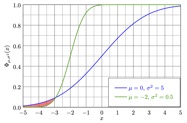
(b) Almost stochastic order, with blue $\succsim$ green.

Figure 1: Examples for stochastic order (a) and almost stochastic order (b), illustrated using the CDFs of two normal random variables. Because stochastic order is too strict to be practical, almost stochastic order allows for some degree of violation of the order (red area in (b)).

with $\mathbbm{1}(\cdot)$ being the indicator function. In practice, since we do not know the real score distributions $p(\operatorname{\mathcal{X}}_{\operatorname{\mathcal{A}}})$ and $p(\operatorname{\mathcal{X}}_{\operatorname{\mathcal{B}}})$, we cannot use the precise CDFs in subsequent calculations, and we rely on the empirical CDFs $F_{n}$ and $G_{m}$. A case of stochastic order is illustrated in Figure 1(a), using the CDFs of two normal distributions. However, in cases such Figure 1(b) we would still like to declare one of the algorithms superior, even though the stochastic order of the underlying CDFs is partially violated. Several ways to quantify the violation of stochastic dominance exist (Álvarez-Esteban et al., 2017; del Barrio et al., 2018a), but here we elaborate on the optimal transport approach by del Barrio et al. (2018b). They propose a the following expression quantifying the distance of each random variables from being stochastically larger than the other:

$$\varepsilon_{W_{2}}(F,G)=\frac{\int_{\mathbb{V}_{\operatorname{\mathcal{X}}}}(F^{-1}(t)-G^{-1}(t))^{2}dt}{(W_{2}(F,G))^{2}}$$ (1)

with the violation ratio $\varepsilon_{W_{2}}(F,G)\in[0,1]$ and a violation set $\mathbb{V}_{\operatorname{\mathcal{X}}}=\big{\{}t\in(0,1):F^{-1}(t)<G^{-1}(t)\big{\}}$, i.e. where the stochastic order is being violated. Equation 1 contains the following components: Firstly, the quantile functions $F^{-1}(t)$ and $G^{-1}(t)$ associated with the correspondng CDFs:

$$F^{-1}(t)=\inf\big{\{}x:t\leq F(x)\big{\}},\quad t\in(0,1)$$

The quantile functions allow us to define stochastic order via $X\succeq Y\iff\forall t\in(0,1):F^{-1}(t)\geq G^{-1}(t)$. Secondly, the univariate $l_{2}$-Wasserstein distance:

$$W_{2}(F,G)=\sqrt{\int_{0}^{1}\big{(}F^{-1}(t)-G^{-1}(t)\big{)}^{2}dt}$$ (2)

Finally, del Barrio et al. (2018b); Dror et al. (2019) define a hypothesis test based on this quantity by formulating the following hypotheses:

$$H_{0}: \varepsilon_{W_{2}}(F,G)\geq\tau$$

$$H_{1}: \varepsilon_{W_{2}}(F,G)<\tau$$

for a pre-defined threshold $\tau>0$, for instance $0.5$ or lower (see discussion in Section B.1 about the choice of threshold). Further, Álvarez-Esteban et al. (2017); Dror et al. (2019) produce a frequentist upper bound to this quantity, defining the minimal $\varepsilon_{W_{2}}$ for which we can reject the null hypothesis with a confidence of $1-\alpha$ as

$$\operatorname{\varepsilon_{\text{min}}}(F_{n},G_{m},\alpha)=\varepsilon_{W_{2}}(F_{n},G_{m})-\sqrt{\frac{n+m}{nm}}\hat{\sigma}_{n,m}\Phi^{-1}(\alpha)$$ (3)

The variance term $\hat{\sigma}_{n,m}$ is estimated using bootstrapping, with $F_{n}^{*}$ and $G_{m}^{*}$ denoting empirical CDFs based on sets of scores resampled from original sets of model scores, similar to re-sampling procedure in other tests like the bootstrap (Efron & Tibshirani, 1994) or permutation-randomization test (Noreen, 1989):

$$\hat{\sigma}_{n,m}^{2}=\text{Var}\bigg{[}\sqrt{\frac{mn}{n+m}}\big{(}\varepsilon_{W_{2}}(F_{n}^{*},G_{m}^{*})-\varepsilon_{W_{2}}(F_{n},G_{m})\big{)}\bigg{]}$$ (4)

Thus, if $\operatorname{\varepsilon_{\text{min}}}(F_{n},G_{m},\alpha)<\tau$, we can reject the null hypothesis and claim that algorithm $\mathbb{A}$ is better than $\mathbb{B}$, with a growing discrepancy in performance the smaller the value becomes. This enables us to pose the following kind of hypotheses:

5 Experimental Comparison with other Tests

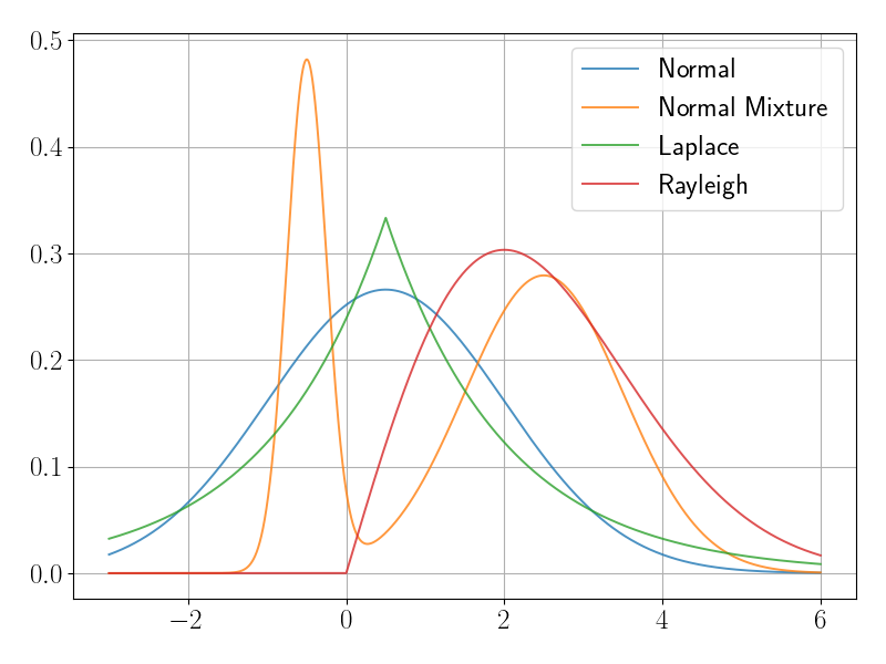
Figure 2: Plot of distributions used for Type I and Type II error tests.

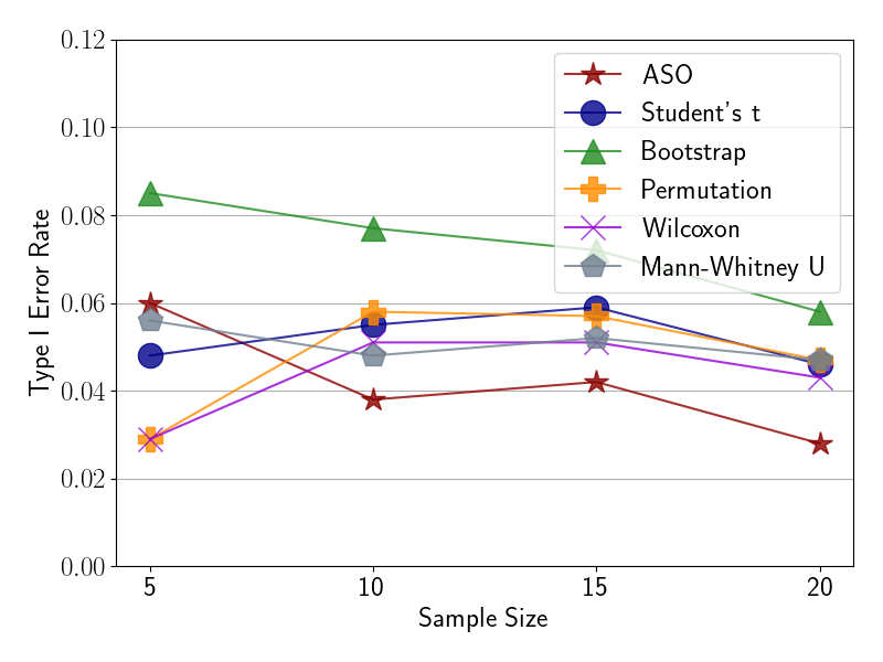
(a) Rates for normal samples.

(b) Rates for normal mixture samples.

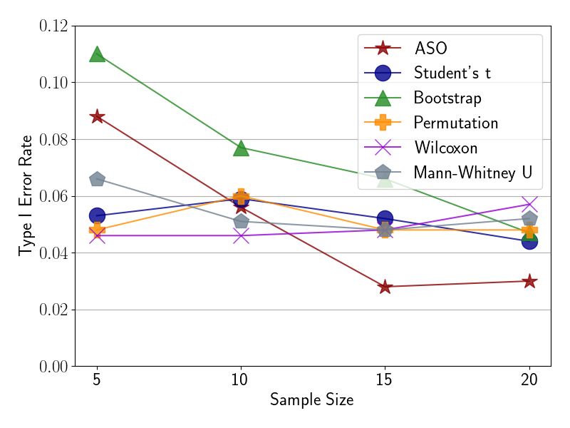
(c) Rates for Laplace samples.

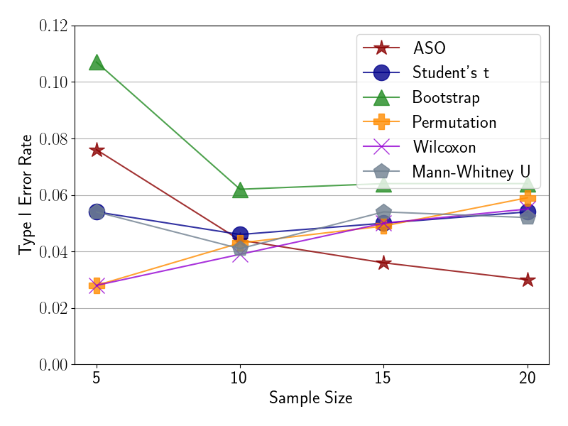
(d) Rates for Rayleigh samples.

Figure 3: Comparing type I error rates for different tests and distributions as a function of sample size. Decisions are made using a confidence threshold of $\alpha=0.05$ and $\tau=0.2$ for $\varepsilon_{\text{min}}$.

We compare ASO to established significance tests such as the Student’s t, the bootstrap (Efron & Tibshirani, 1994), permutation-randomization test (Noreen, 1989) along with the Wilcoxon signed-rank (Wilcoxon, 1992) and Mann-Whitney U test (Mann & Whitney, 1947) on different types of distributions, which are plotted in Figure 2. We plot the Type I error rate per $500$ simulations for ASO and $1000$ simulations for the other tests as a function of sample size in Figure 3, where we sample both sets of observation from the same distribution. For Figure 3(a), we sample from $\mathcal{N}(0,1.5^{2})$ and try a bimodal normal mixture in Figure 3(b) (using the same parameter for the second component, and $\mathcal{N}(-0.5,0.25^{2})$ with mixture weights $\pi_{1}=0.75$ and $\pi_{2}=0.25$). To also test the behavior of tests on non-normal distributions, we also sample from a $\text{Laplace}(0,1.5^{2})$ distribution in Figure 3(c), which posseses a different behavior around the main, as well as the Rayleigh distribution with $\text{Rayleigh}(1)$ in Figure 3(d), which has a heavy tail.

We can see that ASO performs either en par or better than other tests in all scenarios, achieving lower error rates the more samples are available, while other tests score around the expected type I error of $5\%$. In Appendix B, Type II error experiments reveal that the test produces comparatively higher error rates for ASO, though. This can be explained by the fact that we use the upper bound $\operatorname{\varepsilon_{\text{min}}}$ instead of $\varepsilon_{W_{2}}$ to evaluate the null hypothesis, which makes the test act more conservatively. We also find in Appendix B that a decision threshold of $\tau=0.2$ strikes an acceptable balance between Type I and II error rates across different scenarios. Overall, we argue that a lower Type I error is more advantageous in the context of empirical research, and that a decreasing error rate w.r.t. higher sample sizes constitutes an appealing property when used on arbitrary distributions.

In these experiments, the score distributions were determined a priori in order to create rigid experimental conditions. Naturally, a practitioner would not know these distribution in a usual setting, which is why we illustrate the usage of the package the next section.

6 Package Contents & Examples

for tree= grow’=0, child anchor=west, parent anchor=south, anchor=west, calign=first, edge path= [draw, edge] (!u.south west) +(7.5pt,0) |- node[fill,inner sep=1.25pt] (.child anchor)edge label; , before typesetting nodes= if n=1 insert before=[,phantom] , fit=band, before computing xy=l=15pt, [deep-significance [Almost Stochastic Order (ASO) [ASO Significance test: aso()] [ASO for $>3$ sets of scores: multi_aso()] ] [Determining Sample Size [For ASO: aso_uncertainty_reduction()] [Bootstrap Power Analysis: bootstrap_power_analysis()] ] [Classical Significance tests [Bootstrap Test: bootstrap_test()] [Permutation Test: permutation_test()] [Bonferroni Correction: bonferroni_correction()] ] ]

Figure 4: Overview over package contents of deep-significance v1.2.5.

Figure 4 lists the three main groups contents in the package. For one, the package implements some common significance tests, such as the permutation-randomization test (Noreen, 1989) and the bootstrap test (Efron & Tibshirani, 1994), as well as function to perform the Bonferroni correction (Bonferroni, 1936) for multiple comparisons. These tests where chosen because they do not come with any assumptions about the distribution on samples – which also implies low statistical power.

Another part of the package is dedicated to determining the right sample size – aso_uncertainty_reduction() determine the factor by which the uncertainty about the estimate of $\varepsilon_{W_{2}}(F,G)$ is reduced by increasing the size of either sample of scores. Another, more general approach is Bootstrap Power Analysis (Yuan & Hayashi, 2003; Henderson et al., 2018): Each score in the sample is given an equal lift by a constant factor, creating a second, artificial sample. Then, a significance test is run repeatedly on bootstrapped versions of both samples, the percentage of resulting $p$-values under a given threshold is recorded. Ideally, this should result in large number of significant differences induced by the lift – if not, this can be indicate a too high of a variance in the original set of scores. Lastly, the package implements the ASO test from Section 4.1, with more details described in Appendix A.

Quality-of-Life features

To increase ease of use, the package comes with the following features: Scores can be supplied in the most common data types, including Python lists, NumPy (Harris et al., 2020) and JAX arrays (Bradbury et al., 2018), as well as PyTorch (Paszke et al., 2017) and Tensorflow tensors (Abadi et al., 2015). To decrease the waiting time for results, the number of processes can be increases using the num_jobs argument. Furthermore, for comparing more than two samples at once, multi_aso() can be used, which outputs the results in a tabular structure and automatically applies the Bonferroni correction by default. All stochastic functions support seeding for replicability.

Choice of Test

All packaged tests come with weak or no assumption about the score distribution. If the distribution is known, an appropriate parametric test should always be preferred. The bootstrap and permutation test can be used if $p$-values are desired, with the former possessing a higher statistical power. In cases with unusual or unknown score distributions, we recommend ASO, since the only assumptions it makes are that the true CDFs $F$ and $G$ have bounded convex support and their underlying PDFs to have finite second order moments.

6.1 Case study – Deep Q-Learning

In order to demonstrate the intended use of the package, we showcase its use in a case study, based on the simple Reinforcement Learning described below. Here, reward distributions are usually not normal, and therefore provide an ideal testbed. All used code is available in the repository.

We tackle the problem above with a classic Deep Reinforcement Learning approach, namely Deep Q-Learning (Mnih et al., 2015). Deep Q-Learning tries to approximate the optimal action-value function defined as

$$Q^{*}(s,a)=\max_{\pi}\mathbb{E}\big{[}r_{t}+\gamma r_{t+1}+\gamma^{2}r_{t+2}+\ldots\big{|}s_{t}=s,a_{t}=a,\pi\big{]}$$

The definition above reads as follow: The optimal action-value function is the policy $\pi$ that maximizes the future reward $r_{t}$ at a state $s_{t}$ by performing an action $a_{t}$, with subsequent rewards being increasingly discounted by a factor $\gamma$. The model weights are updated using the following $l_{2}$ loss:

$$\mathcal{L}(\theta)=\mathbb{E}_{(s,a,r,s^{\prime})\sim U(\text{Buffer})}\bigg{[}\Big{(}r+\max_{a^{\prime}}Q(s^{\prime},a^{\prime};\theta^{\text{target}})-Q(s,a;\theta)\Big{)}^{2}\bigg{]}$$

Two aspects of this loss function are especially noteworthy: First of all, since we do not know the true value of the $Q$-function in most cases, the predicted value $Q(s,a;\theta)$ is compared against the reward plus outcome of the greedy action chosen by a target network: To avoid having to “hit a moving target” (Van Hasselt et al., 2018), the target network is only updated every couple of training steps by copying the main networks parameters. Secondly, the state, action and reward used to compute the loss are not the ones just observed by the model, but instead are uniformly sampled from a replay buffer, a sort of memory that past experiences gets added to during training.

In our example, we investigate how the update frequency of the target network affects the mean of the rewards obtained during training. First, we train five models with an update frequency of $10$ and $20$ steps each, and store the results. But how do we know that we collected enough scores to make a meaningful comparison? The package supplies two functions for this purpose, the first of which is an implementation of bootstrap power analysis (Yuan & Hayashi, 2003) shown below:

⬇

from deepsig import bootstrap_power_analysis

\parbootstrap_power_analysis(reward_dist_freq_10, num_jobs=4) # Results for 10 steps, gives 0.6594

bootstrap_power_analysis(reward_dist_freq_20, num_jobs=4) # Results for 20 steps, gives 0.5616

These scores have a direct statistical interpretation, since they signify the statistical power. The higher the statistical power, the lower the probability of a Type II error or false negative. A common rule of thumb is to thrive for a power of around $0.8$, and we might therefore want to collect more samples here. For instance, we could decide to collect $10$ or $15$ samples in total. In case we are using the ASO test, the second function can help with this decision:

⬇

from deepsig import aso_uncertainty_reduction

\paraso_uncertainty_reduction(m_old=5, n_old=5, m_new=10, n_new=10) # 1.414

aso_uncertainty_reduction(m_old=5, n_old=5, m_new=15, n_new=15) # 1.732

Since ASO only computes the “true” $\varepsilon_{\text{min}}$ value in the limit of infinitely large samples, the estimate obtained using bootstrapping has some inherent variance, which can be reduced by adding more scores to the sample. The function above computes the factor by which the uncertainty in the test result is being reduced. We can thus read the above as adding five more samples reducing the uncertainty by a factor of $1.41$, while adding ten more sample only reduces it by $1.73$. To strike a compromise with our computational budget, we decide to only add five more samples each and run two of the implemented tests:

⬇

from deepsig import aso, bootstrap_test

\paraso(rewards_freq_10, rewards_freq_20, num_jobs=4) # 0.02

bootstrap_test(rewards_freq_10, rewards_freq_20, num_jobs=4) # 0.005

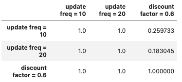
Figure 5: Results of demo.

These results suggest that an update frequency of $10$ works is superior. Lastly, we can easily facilitate comparisons between multiple models using the multi_aso() function below. By supplying scores in dictionary form and specifying return_df=True, the results will be returned in an easily readable pandas DataFrame. Furthermore, the Bonferroni correction (Bonferroni, 1936) is being applied automatically to avoid the multiple comparisons problem.

⬇

res_df = multi_aso(

{

"update freq = 10": reward_dist_freq_10,

"update freq = 20": reward_dist_freq_20,

"discount factor = 0.6": reward_dist_discount_06

},

num_jobs=4, return_df=True

)

Overall, the results in the demonstration shown in Figure 5 that an update frequency of ten steps performed best, and that using a lower discount factor produced worse results.

7 Discussion

The previous sections have demonstrated the advantages of the implemented tests in an neural network setting. Furthermore, the package implements other useful functions that can be used to evaluate experimental settings. Nevertheless, using these techniques in practice comes with limitations as well, which the end user should be aware of.

The first line of limits comes with ASO itself. Multiple steps of the procedure require different kinds of approximations or properties that are only guaranteed to hold in the infinite-sample limit , e.g. Equation 4. Furthermore, significance tests in general are known to sometimes provide unreliable results with small (Reimers & Gurevych, 2018) or very large sample sizes (Lin et al., 2013), are prone to misinterpretation (Gibson, 2021; Greenland et al., 2016), and encourages binary significant / non-significant thinking (Wasserstein et al., 2019; Azer et al., 2020). An attractive alternative to statistical hypothesis testing therefore comes in the form of Bayesian analysis (Kruschke, 2013; Benavoli et al., 2017; Gelman et al., 2021), where the user draws conclusions from posterior distributions over quantities of interest. A potential drawback of this methodology is that it often comes at the cost of having to use Markov Chain Monte Carlo methods, and requiring experience from the user with checking convergence and defining appropriate models and model priors.

8 Conclusion

This work has presented an open-source software package implementing several useful tools to evaluate experimental results for Deep Neural Networks, including the ASO test by del Barrio et al. (2018b); Dror et al. (2019). We demonstrated their usefulness in a case study and discussed potential shortcomings and pitfalls. We see this package as a valuable contribution to improve experimental rigour in Machine Learning, while maintaining accessibility and ease of use. Future work could for instance derive more robust estimations of the violation ratio for small sample sizes, or come up with reliable and general Bayesian tests to evaluate experiments.

Appendix A Implementation Details

Data: Sets of observations $\mathbb{S}_{\mathbb{A}}$ and $\mathbb{S}_{\mathbb{B}}$, integration interval $\Delta_{t}$, number of bootstrap iterations $B$, desired confidence level $1-\alpha$.

Result: Upper bound to violation ration $\operatorname{\varepsilon_{\text{min}}}$.

$\varepsilon_{\mathcal{W}_{2}}(F_{n},G_{m})$ = compute_violation_ratio($\mathbb{S}_{\mathbb{A}}$, $\mathbb{S}_{\mathbb{A}}$, $\Delta_{t}$)

// Bootstrapping

for $i\in\ 0,\ldots,B$ do

       $\mathbb{S}_{\mathbb{A}}^{*}=$ bootstrap_sample($\mathbb{S}_{\mathbb{A}}$)

       $\mathbb{S}_{\mathbb{B}}^{*}=$ bootstrap_sample($\mathbb{S}_{\mathbb{B}}$)

      

       // Store value below in list

       $\varepsilon^{*}_{\mathcal{W}_{2}}(F_{n},G_{m})$ = compute_violation_ratio($\mathbb{S}_{\mathbb{A}}^{*}$, $\mathbb{S}_{\mathbb{A}}^{*}$, $\Delta_{t}$)

      

end for

// Compute value below based on variance of all the $\varepsilon_{\mathcal{W}_{2}}^{*}$ in list

$\hat{\sigma}_{n,m}^{2}=\text{Var}\bigg{[}\sqrt{\frac{mn}{n+m}}\big{(}\varepsilon_{W_{2}}(F_{n}^{*},G_{m}^{*})-\varepsilon_{W_{2}}(F_{n},G_{m})\big{)}\bigg{]}$

$\operatorname{\varepsilon_{\text{min}}}(F_{n},G_{m},\alpha)=\varepsilon_{W_{2}}(F_{n},G_{m})-\sqrt{\frac{n+m}{nm}}\hat{\sigma}_{n,m}\Phi^{-1}(\alpha)$

Algorithm 1 Almost Stochastic Order (ASO) Significance Test

The full algorithm to compute the $\operatorname{\varepsilon_{\text{min}}}$ score is given in Algorithm 1, and will now be explained in full detail. We show how the violation ratio in Equation 1 can be compute in Python:

⬇

def compute_violation_ratio(scores_a: np.array, scores_b: np.array, dt: float) -> float:

quantile_func_a = get_quantile_function(scores_a)

quantile_func_b = get_quantile_function(scores_b)

\part = np.arange(dt, 1, dt) # Points we integrate over

f = quantile_func_a(t) # F-1(t)

g = quantile_func_b(t) # G-1(t)

diff = g - f

squared_wasserstein_dist = np.sum(diff ** 2 * dt)

\par# Now only consider points where stochastic order is being violated and set the rest to 0

diff[f >= g] = 0

int_violation_set = np.sum(diff[1:] ** 2 * dt) # Ignore t = 0 since t in (0, 1)

\parviolation_ratio = int_violation_set / squared_wasserstein_dist

\parreturn violation_ratio

We can see that the integration over the violation set $\mathbb{V}_{X}$ in Equation 1 is being performed by masking out values for which the stochastic order is honored (i.e. where $F_{n}^{-1}(t)\geq G_{n}^{-1}(t)$. Computing the violation ratio involves building the empirical inverse cumulative distribution function or empircial quantile function, the same method as in Dror et al. (2019) is used, with the corresponding Python code given below:

⬇

def get_quantile_function(scores: np.array) -> Callable:

def _quantile_function(p: float) -> float:

cdf = np.sort(scores)

num = len(scores)

index = int(np.ceil(num * p))

\parreturn cdf[np.clip(index - 1, 0, num - 1))]

\parreturn np.vectorize(_quantile_function)

This function is also used inside the bootstrap sampling procedure, the last missing part of the implementation. We again follow the implementation by Dror et al. (2019) and employ the inverse transform sampling procedure, in which we draw $p\sim\mathcal{U}[0,1]$ and run it through a quantile function to create a sample.

Appendix B Experimental Appendix

B.1 Additional Error Rate Experiments

(a) Dists. for normal samples.

(b) Dists. for normal mixture samples.

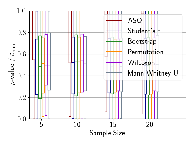
(c) Dists. for Laplace samples.

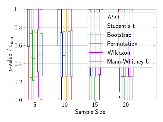
(d) Dists. for Rayleigh samples.

Figure 6: Comparing test score distributions for different tests and distributions as a function of sample size.

We use this section to further shed light on the results in Figure 3.

Test score distributions

Instead of showing the Type I error rates based on thresholded test results, we instead plot the distributions over test scores in Figure 6. We can observe that the lower ends of the interquartile range of $\operatorname{\varepsilon_{\text{min}}}$ distributions are either the same or higher than the ones for $p$-values (they do not need to be centered around $0.5$ since $\operatorname{\varepsilon_{\text{min}}}$ is an upper bound to $\varepsilon_{W_{2}}$), explaining the lower Type I error rate.

(a) Type II error as a function of sample size.

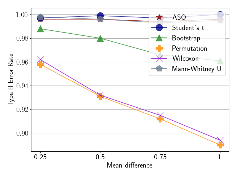
(b) Type II error rate as a function of mean difference.

(c) Type II error as a function of sample size.

(d) Type II error rate as a function of mean difference.

Figure 7: Measuring the Type II error rate of the considered tests on normal and normal mixture distributions as a function of sample size Figures 7(a) and 7(c) and mean differences Figures 7(b) and 7(d).

Type II error rate experiments

We furthermore test the Type II error rates on samples from different distributions in Figure 7, sampling the score samples $500$ times for ASO and $1000$ times for the other tests from $\mathcal{N}(0.5,1.5^{2})$ and $\mathcal{N}(0,1.5^{2})$, respectively, for a $p$-value threshold of $0.05$ and $\operatorname{\varepsilon_{\text{min}}}$ threshold of $0.2$. We see that the Type II error rate decreases with increasing sample size (Figures 7(a) and 7(c)), but is less sensitive for increasing mean difference than other tests (Figures 7(b) and 7(d)). Generally, we can observe the behavior to be very similar to Student’s t and Mann-Whitney U test.

Error rates by rejection threshold

Lastly, we report the Type I and II error rates on the tested distributions using different Type I / II error rates. In Tables 1, 4, 7 and 8, we see that ASO achieves lower error rates than other tests in almost all scenarios when faced with the fame threshold. Naturally, these thresholds cannot be interpreted the same for ASO and the other significance tests. Nevertheless, we can see that a threshold of $\tau=0.2$ seems to roughly correspond to a $p$-value threshold of $0.05$ in terms of Type I error rate. Type II error rates are given in Tables 2, 3, 5 and 6. Here the difference between ASO and the other tests is not quite as pronounced, however, it always incurs higher error rates.

Table 1: Type I error rates for samples drawn from a normal distribution as a function of sample size and different rejection thresholds.

Sample Size	Threshold	ASO	Student’s t	Bootstrap	Permutation	Wilcoxon	Mann-Whitney U
5	0.05	0.02	0.048	0.085	0.029	0.029	0.056
	0.10	0.034	0.093	0.149	0.079	0.088	0.085
	0.20	0.06	0.212	0.241	0.197	0.16	0.159
	0.30	0.094	0.299	0.322	0.286	0.236	0.284
	0.40	0.146	0.396	0.403	0.37	0.315	0.348
	0.50	0.216	0.483	0.483	0.468	0.49	0.498
10	0.05	0.004	0.055	0.077	0.058	0.051	0.048
	0.10	0.014	0.103	0.13	0.11	0.113	0.1
	0.20	0.038	0.196	0.215	0.201	0.192	0.194
	0.30	0.084	0.282	0.3	0.285	0.261	0.272
	0.40	0.138	0.394	0.398	0.395	0.387	0.378
	0.50	0.204	0.49	0.486	0.491	0.499	0.479
15	0.05	0.002	0.059	0.072	0.057	0.051	0.052
	0.10	0.014	0.106	0.123	0.104	0.095	0.113
	0.20	0.042	0.198	0.215	0.199	0.186	0.196
	0.30	0.08	0.303	0.309	0.303	0.295	0.304
	0.40	0.136	0.395	0.4	0.392	0.371	0.368
	0.50	0.19	0.482	0.485	0.479	0.47	0.468
20	0.05	0.004	0.046	0.058	0.047	0.043	0.047
	0.10	0.006	0.095	0.105	0.093	0.085	0.092
	0.20	0.028	0.181	0.196	0.177	0.171	0.183
	0.30	0.074	0.28	0.29	0.289	0.284	0.273
	0.40	0.12	0.384	0.389	0.381	0.372	0.394
	0.50	0.17	0.479	0.478	0.473	0.477	0.481

Table 2: Type II error rates for samples drawn from two different normal distributions as a function of sample size and different rejection thresholds.

Sample Size	Threshold	ASO	Student’s t	Bootstrap	Permutation	Wilcoxon	Mann-Whitney U
5	0.05	0.942	0.883	0.796	0.918	0.925	0.875
	0.10	0.916	0.786	0.714	0.802	0.792	0.819
	0.20	0.87	0.623	0.585	0.649	0.691	0.694
	0.30	0.792	0.512	0.48	0.521	0.597	0.539
	0.40	0.714	0.399	0.39	0.421	0.498	0.47
	0.50	0.65	0.302	0.315	0.318	0.387	0.391
10	0.05	0.978	0.836	0.791	0.853	0.864	0.84
	0.10	0.95	0.73	0.695	0.737	0.743	0.741
	0.20	0.868	0.58	0.551	0.58	0.595	0.576
	0.30	0.802	0.428	0.41	0.429	0.462	0.453
	0.40	0.708	0.33	0.328	0.327	0.347	0.329
	0.50	0.604	0.223	0.223	0.229	0.272	0.251
15	0.05	0.984	0.769	0.734	0.781	0.788	0.787
	0.10	0.95	0.643	0.615	0.646	0.672	0.639
	0.20	0.84	0.47	0.455	0.48	0.493	0.481
	0.30	0.716	0.348	0.34	0.35	0.355	0.365
	0.40	0.61	0.244	0.245	0.246	0.276	0.261
	0.50	0.486	0.177	0.176	0.175	0.185	0.192
20	0.05	0.976	0.732	0.709	0.736	0.75	0.747
	0.10	0.946	0.601	0.586	0.601	0.614	0.61
	0.20	0.848	0.406	0.396	0.41	0.421	0.41
	0.30	0.704	0.277	0.268	0.272	0.299	0.289
	0.40	0.58	0.2	0.201	0.198	0.221	0.206
	0.50	0.444	0.144	0.144	0.147	0.156	0.152

Table 3: Type II error rates for samples drawn from a normal distribution as a function of mean difference and different rejection thresholds.

Difference	Treshold	ASO	Student’s t	Bootstrap	Permutation	Wilcoxon	Mann-Whitney U
0.25	0.05	0.984	0.925	0.857	0.941	0.945	0.93
	0.10	0.954	0.846	0.781	0.859	0.844	0.881
	0.20	0.914	0.705	0.659	0.721	0.761	0.768
	0.30	0.872	0.585	0.554	0.606	0.68	0.622
	0.40	0.8	0.482	0.462	0.489	0.594	0.548
	0.50	0.714	0.381	0.387	0.394	0.48	0.465
0.50	0.05	0.966	0.888	0.805	0.918	0.92	0.883
	0.10	0.932	0.784	0.7	0.811	0.794	0.83
	0.20	0.87	0.616	0.57	0.652	0.696	0.698
	0.30	0.812	0.5	0.477	0.523	0.602	0.535
	0.40	0.722	0.406	0.397	0.426	0.505	0.466
	0.50	0.606	0.313	0.315	0.326	0.411	0.401
0.75	0.05	0.934	0.822	0.707	0.883	0.885	0.822
	0.10	0.896	0.699	0.61	0.725	0.71	0.764
	0.20	0.798	0.514	0.469	0.561	0.599	0.607
	0.30	0.702	0.407	0.37	0.421	0.515	0.455
	0.40	0.59	0.308	0.3	0.325	0.406	0.375
	0.50	0.482	0.223	0.222	0.237	0.303	0.295
1.00	0.05	0.87	0.739	0.609	0.85	0.85	0.743
	0.10	0.796	0.585	0.488	0.678	0.655	0.659
	0.20	0.712	0.386	0.327	0.449	0.497	0.487
	0.30	0.58	0.257	0.232	0.289	0.388	0.307
	0.40	0.504	0.178	0.17	0.194	0.278	0.229
	0.50	0.384	0.115	0.115	0.128	0.189	0.176

Table 4: Type I error rates for samples drawn from a normal mixture distribution as a function of sample size and different rejection thresholds.

Sample Size	Threshold	ASO	Student’s t	Bootstrap	Permutation	Wilcoxon	Mann-Whitney U
5	0.05	0.0	0.0	0.012	0.028	0.026	0.003
	0.10	0.0	0.013	0.035	0.079	0.085	0.004
	0.20	0.0	0.069	0.104	0.179	0.153	0.049
	0.30	0.008	0.169	0.213	0.281	0.208	0.16
	0.40	0.024	0.338	0.358	0.363	0.305	0.244
	0.50	0.058	0.494	0.493	0.483	0.484	0.478
10	0.05	0.0	0.007	0.018	0.059	0.049	0.011
	0.10	0.0	0.031	0.05	0.11	0.109	0.03
	0.20	0.004	0.102	0.121	0.205	0.188	0.109
	0.30	0.008	0.221	0.229	0.302	0.273	0.211
	0.40	0.034	0.347	0.349	0.398	0.379	0.351
	0.50	0.07	0.511	0.515	0.506	0.491	0.495
15	0.05	0.0	0.006	0.007	0.055	0.048	0.004
	0.10	0.0	0.022	0.033	0.106	0.097	0.017
	0.20	0.002	0.103	0.118	0.194	0.202	0.095
	0.30	0.006	0.215	0.22	0.301	0.308	0.208
	0.40	0.028	0.356	0.366	0.415	0.404	0.328
	0.50	0.082	0.501	0.499	0.496	0.502	0.501
20	0.05	0.0	0.006	0.007	0.048	0.045	0.005
	0.10	0.0	0.019	0.027	0.088	0.085	0.021
	0.20	0.0	0.104	0.109	0.2	0.187	0.097
	0.30	0.006	0.214	0.218	0.307	0.289	0.221
	0.40	0.032	0.363	0.369	0.412	0.39	0.349
	0.50	0.082	0.494	0.495	0.492	0.496	0.485

Table 5: Type II error rates for samples drawn from two normal mixture distribution as a function of sample size and different rejection thresholds.

Sample Size	Threshold	ASO	Student’s t	Bootstrap	Permutation	Wilcoxon	Mann-Whitney U
5	0.05	1.0	0.999	0.964	0.892	0.897	0.995
	0.10	1.0	0.962	0.874	0.728	0.697	0.985
	0.20	0.994	0.747	0.64	0.474	0.525	0.87
	0.30	0.976	0.476	0.422	0.299	0.426	0.579
	0.40	0.896	0.252	0.234	0.206	0.326	0.414
	0.50	0.748	0.117	0.118	0.122	0.222	0.28
10	0.05	1.0	0.908	0.831	0.552	0.635	0.926
	0.10	0.996	0.721	0.641	0.354	0.419	0.73
	0.20	0.954	0.39	0.354	0.186	0.247	0.407
	0.30	0.828	0.191	0.18	0.108	0.156	0.219
	0.40	0.642	0.089	0.087	0.068	0.089	0.107
	0.50	0.452	0.034	0.031	0.037	0.056	0.052
15	0.05	0.996	0.829	0.757	0.352	0.441	0.864
	0.10	0.99	0.568	0.517	0.213	0.272	0.628
	0.20	0.928	0.251	0.234	0.087	0.129	0.298
	0.30	0.774	0.099	0.091	0.033	0.058	0.116
	0.40	0.498	0.027	0.026	0.019	0.034	0.044
	0.50	0.276	0.009	0.01	0.01	0.013	0.014
20	0.05	1.0	0.653	0.58	0.204	0.279	0.666
	0.10	0.98	0.359	0.333	0.105	0.162	0.392
	0.20	0.848	0.107	0.101	0.035	0.064	0.147
	0.30	0.586	0.038	0.035	0.013	0.022	0.047
	0.40	0.344	0.01	0.01	0.008	0.013	0.017
	0.50	0.13	0.003	0.003	0.004	0.006	0.006

Table 6: Type II error rates for samples drawn from two normal mixture distribution as a function of mean difference between two of the mixture components and different rejection thresholds.

		ASO	Student’s t	Bootstrap	Permutation	Wilcoxon	Mann-Whitney U
diff	threshold
0.25	0.05	1.0	0.997	0.988	0.958	0.962	0.998
	0.10	0.998	0.988	0.96	0.894	0.882	0.994
	0.20	0.996	0.903	0.856	0.754	0.792	0.945
	0.30	0.978	0.762	0.727	0.643	0.724	0.814
	0.40	0.94	0.594	0.576	0.53	0.621	0.704
	0.50	0.886	0.424	0.424	0.444	0.532	0.563
0.50	0.05	0.998	0.999	0.98	0.931	0.932	0.996
	0.10	0.998	0.978	0.931	0.82	0.802	0.99
	0.20	0.996	0.849	0.775	0.647	0.695	0.905
	0.30	0.976	0.659	0.603	0.511	0.611	0.724
	0.40	0.928	0.458	0.438	0.407	0.504	0.577
	0.50	0.84	0.284	0.287	0.31	0.395	0.449
0.75	0.05	1.0	0.997	0.966	0.912	0.915	0.993
	0.10	0.998	0.966	0.901	0.769	0.746	0.985
	0.20	0.994	0.802	0.707	0.553	0.623	0.886
	0.30	0.974	0.547	0.497	0.397	0.516	0.651
	0.40	0.922	0.355	0.337	0.286	0.407	0.485
	0.50	0.824	0.191	0.191	0.198	0.305	0.363
1.00	0.05	1.0	1.0	0.961	0.89	0.894	0.995
	0.10	1.0	0.958	0.868	0.714	0.682	0.989
	0.20	0.996	0.715	0.617	0.445	0.505	0.872
	0.30	0.962	0.432	0.38	0.291	0.419	0.545
	0.40	0.87	0.253	0.235	0.204	0.308	0.408
	0.50	0.702	0.12	0.12	0.132	0.208	0.263

Table 7: Type I error rates for samples drawn from a Laplace distribution as a function of sample size and different rejection thresholds.

Sample Size	Threshold	ASO	Student’s t	Bootstrap	Permutation	Wilcoxon	Mann-Whitney U
5	0.05	0.022	0.053	0.11	0.048	0.046	0.066
	0.10	0.038	0.117	0.164	0.106	0.116	0.097
	0.20	0.088	0.223	0.261	0.208	0.187	0.169
	0.30	0.124	0.319	0.343	0.295	0.234	0.286
	0.40	0.154	0.427	0.445	0.398	0.322	0.379
	0.50	0.218	0.509	0.51	0.491	0.506	0.508
10	0.05	0.004	0.059	0.077	0.06	0.046	0.051
	0.10	0.012	0.114	0.142	0.111	0.106	0.098
	0.20	0.056	0.218	0.236	0.216	0.202	0.199
	0.30	0.104	0.314	0.33	0.318	0.29	0.291
	0.40	0.164	0.404	0.407	0.398	0.378	0.4
	0.50	0.238	0.475	0.475	0.473	0.481	0.486
15	0.05	0.0	0.052	0.066	0.048	0.048	0.048
	0.10	0.012	0.1	0.117	0.103	0.1	0.101
	0.20	0.028	0.204	0.22	0.199	0.199	0.187
	0.30	0.07	0.311	0.319	0.303	0.296	0.294
	0.40	0.12	0.404	0.409	0.402	0.378	0.394
	0.50	0.194	0.51	0.514	0.511	0.504	0.519
20	0.05	0.004	0.044	0.047	0.048	0.057	0.052
	0.10	0.01	0.099	0.113	0.104	0.103	0.101
	0.20	0.03	0.214	0.232	0.215	0.199	0.202
	0.30	0.064	0.312	0.325	0.308	0.297	0.307
	0.40	0.138	0.414	0.413	0.415	0.381	0.405
	0.50	0.22	0.507	0.505	0.501	0.485	0.496

Table 8: Type I error rates for samples drawn from a Rayleigh distribution as a function of sample size and different rejection thresholds.

Sample Size	Threshold	ASO	Student’s t	Bootstrap	Permutation	Wilcoxon	Mann-Whitney U
5	0.05	0.012	0.054	0.107	0.028	0.028	0.054
	0.10	0.034	0.108	0.147	0.089	0.096	0.088
	0.20	0.076	0.203	0.235	0.187	0.162	0.165
	0.30	0.11	0.319	0.342	0.302	0.229	0.291
	0.40	0.146	0.423	0.435	0.415	0.331	0.36
	0.50	0.198	0.532	0.539	0.523	0.53	0.524
10	0.05	0.012	0.046	0.062	0.043	0.039	0.041
	0.10	0.018	0.087	0.107	0.093	0.094	0.084
	0.20	0.044	0.187	0.206	0.18	0.172	0.187
	0.30	0.064	0.295	0.314	0.297	0.265	0.284
	0.40	0.114	0.401	0.405	0.399	0.373	0.412
	0.50	0.18	0.507	0.514	0.505	0.5	0.508
15	0.05	0.004	0.05	0.064	0.049	0.05	0.054
	0.10	0.01	0.1	0.115	0.1	0.103	0.104
	0.20	0.036	0.194	0.201	0.182	0.187	0.187
	0.30	0.07	0.295	0.302	0.287	0.294	0.291
	0.40	0.114	0.386	0.394	0.379	0.371	0.373
	0.50	0.198	0.481	0.484	0.487	0.472	0.497
20	0.05	0.002	0.054	0.064	0.059	0.055	0.052
	0.10	0.004	0.115	0.121	0.113	0.103	0.113
	0.20	0.03	0.195	0.205	0.202	0.187	0.204
	0.30	0.058	0.281	0.287	0.277	0.283	0.291
	0.40	0.13	0.377	0.386	0.375	0.368	0.384
	0.50	0.19	0.489	0.493	0.493	0.468	0.469

References

- Abadi et al. (2015) Martín Abadi, Ashish Agarwal, Paul Barham, Eugene Brevdo, Zhifeng Chen, Craig Citro, Greg S. Corrado, Andy Davis, Jeffrey Dean, Matthieu Devin, Sanjay Ghemawat, Ian Goodfellow, Andrew Harp, Geoffrey Irving, Michael Isard, Yangqing Jia, Rafal Jozefowicz, Lukasz Kaiser, Manjunath Kudlur, Josh Levenberg, Dandelion Mané, Rajat Monga, Sherry Moore, Derek Murray, Chris Olah, Mike Schuster, Jonathon Shlens, Benoit Steiner, Ilya Sutskever, Kunal Talwar, Paul Tucker, Vincent Vanhoucke, Vijay Vasudevan, Fernanda Viégas, Oriol Vinyals, Pete Warden, Martin Wattenberg, Martin Wicke, Yuan Yu, and Xiaoqiang Zheng. TensorFlow: Large-scale machine learning on heterogeneous systems, 2015. URL https://www.tensorflow.org/. Software available from tensorflow.org.
- Agarwal et al. (2021) Rishabh Agarwal, Max Schwarzer, Pablo Samuel Castro, Aaron Courville, and Marc G Bellemare. Deep reinforcement learning at the edge of the statistical precipice. arXiv preprint arXiv:2108.13264, 2021.
- Álvarez-Esteban et al. (2017) PC Álvarez-Esteban, Eustasio del Barrio, Juan Antonio Cuesta-Albertos, and C Matrán. Models for the assessment of treatment improvement: The ideal and the feasible. Statistical Science, 32(3):469–485, 2017.
- Azer et al. (2020) Erfan Sadeqi Azer, Daniel Khashabi, Ashish Sabharwal, and Dan Roth. Not all claims are created equal: Choosing the right statistical approach to assess hypotheses. In Dan Jurafsky, Joyce Chai, Natalie Schluter, and Joel R. Tetreault (eds.), Proceedings of the 58th Annual Meeting of the Association for Computational Linguistics, ACL 2020, Online, July 5-10, 2020, pp. 5715–5725. Association for Computational Linguistics, 2020. doi: 10.18653/v1/2020.acl-main.506. URL https://doi.org/10.18653/v1/2020.acl-main.506.
- Barto et al. (1983) Andrew G Barto, Richard S Sutton, and Charles W Anderson. Neuronlike adaptive elements that can solve difficult learning control problems. IEEE transactions on systems, man, and cybernetics, (5):834–846, 1983.
- Benavoli et al. (2017) Alessio Benavoli, Giorgio Corani, Janez Demšar, and Marco Zaffalon. Time for a change: a tutorial for comparing multiple classifiers through bayesian analysis. The Journal of Machine Learning Research, 18(1):2653–2688, 2017.
- Berg-Kirkpatrick et al. (2012) Taylor Berg-Kirkpatrick, David Burkett, and Dan Klein. An empirical investigation of statistical significance in NLP. In Jun’ichi Tsujii, James Henderson, and Marius Pasca (eds.), Proceedings of the 2012 Joint Conference on Empirical Methods in Natural Language Processing and Computational Natural Language Learning, EMNLP-CoNLL 2012, July 12-14, 2012, Jeju Island, Korea, pp. 995–1005. ACL, 2012. URL https://aclanthology.org/D12-1091/.
- Bonferroni (1936) Carlo Bonferroni. Teoria statistica delle classi e calcolo delle probabilita. Pubblicazioni del R Istituto Superiore di Scienze Economiche e Commericiali di Firenze, 8:3–62, 1936.
- Bouthillier et al. (2021) Xavier Bouthillier, Pierre Delaunay, Mirko Bronzi, Assya Trofimov, Brennan Nichyporuk, Justin Szeto, Nazanin Mohammadi Sepahvand, Edward Raff, Kanika Madan, Vikram Voleti, et al. Accounting for variance in machine learning benchmarks. Proceedings of Machine Learning and Systems, 3, 2021.
- Bradbury et al. (2018) James Bradbury, Roy Frostig, Peter Hawkins, Matthew James Johnson, Chris Leary, Dougal Maclaurin, George Necula, Adam Paszke, Jake VanderPlas, Skye Wanderman-Milne, and Qiao Zhang. JAX: composable transformations of Python+NumPy programs, 2018. URL http://github.com/google/jax.
- Brockman et al. (2016) Greg Brockman, Vicki Cheung, Ludwig Pettersson, Jonas Schneider, John Schulman, Jie Tang, and Wojciech Zaremba. Openai gym, 2016.
- Card et al. (2020) Dallas Card, Peter Henderson, Urvashi Khandelwal, Robin Jia, Kyle Mahowald, and Dan Jurafsky. With little power comes great responsibility. In Bonnie Webber, Trevor Cohn, Yulan He, and Yang Liu (eds.), Proceedings of the 2020 Conference on Empirical Methods in Natural Language Processing, EMNLP 2020, Online, November 16-20, 2020, pp. 9263–9274. Association for Computational Linguistics, 2020. doi: 10.18653/v1/2020.emnlp-main.745. URL https://doi.org/10.18653/v1/2020.emnlp-main.745.
- Cooper et al. (2021) A Feder Cooper, Yucheng Lu, Jessica Forde, and Christopher M De Sa. Hyperparameter optimization is deceiving us, and how to stop it. Advances in Neural Information Processing Systems, 34, 2021.
- Dehghani et al. (2021) Mostafa Dehghani, Yi Tay, Alexey A Gritsenko, Zhe Zhao, Neil Houlsby, Fernando Diaz, Donald Metzler, and Oriol Vinyals. The benchmark lottery. arXiv preprint arXiv:2107.07002, 2021.
- del Barrio et al. (2018a) E del Barrio, JA Cuesta-Albertos, and C Matrán. Some indices to measure departures from stochastic order. arXiv preprint arXiv:1804.02905, 2018a.
- del Barrio et al. (2018b) Eustasio del Barrio, Juan A Cuesta-Albertos, and Carlos Matrán. An optimal transportation approach for assessing almost stochastic order. In The Mathematics of the Uncertain, pp. 33–44. Springer, 2018b.
- Dodge et al. (2019) Jesse Dodge, Suchin Gururangan, Dallas Card, Roy Schwartz, and Noah A. Smith. Show your work: Improved reporting of experimental results. In Kentaro Inui, Jing Jiang, Vincent Ng, and Xiaojun Wan (eds.), Proceedings of the 2019 Conference on Empirical Methods in Natural Language Processing and the 9th International Joint Conference on Natural Language Processing, EMNLP-IJCNLP 2019, Hong Kong, China, November 3-7, 2019, pp. 2185–2194. Association for Computational Linguistics, 2019. doi: 10.18653/v1/D19-1224. URL https://doi.org/10.18653/v1/D19-1224.
- Dosovitskiy et al. (2021) Alexey Dosovitskiy, Lucas Beyer, Alexander Kolesnikov, Dirk Weissenborn, Xiaohua Zhai, Thomas Unterthiner, Mostafa Dehghani, Matthias Minderer, Georg Heigold, Sylvain Gelly, Jakob Uszkoreit, and Neil Houlsby. An image is worth 16x16 words: Transformers for image recognition at scale. In 9th International Conference on Learning Representations, ICLR 2021, Virtual Event, Austria, May 3-7, 2021. OpenReview.net, 2021. URL https://openreview.net/forum?id=YicbFdNTTy.
- Dror et al. (2018) Rotem Dror, Gili Baumer, Segev Shlomov, and Roi Reichart. The hitchhiker’s guide to testing statistical significance in natural language processing. In Proceedings of the 56th Annual Meeting of the Association for Computational Linguistics (Volume 1: Long Papers), pp. 1383–1392, 2018.
- Dror et al. (2019) Rotem Dror, Segev Shlomov, and Roi Reichart. Deep dominance - how to properly compare deep neural models. In Anna Korhonen, David R. Traum, and Lluís Màrquez (eds.), Proceedings of the 57th Conference of the Association for Computational Linguistics, ACL 2019, Florence, Italy, July 28- August 2, 2019, Volume 1: Long Papers, pp. 2773–2785. Association for Computational Linguistics, 2019. doi: 10.18653/v1/p19-1266. URL https://doi.org/10.18653/v1/p19-1266.
- Dror et al. (2020) Rotem Dror, Lotem Peled-Cohen, Segev Shlomov, and Roi Reichart. Statistical significance testing for natural language processing. Synthesis Lectures on Human Language Technologies, 13(2):1–116, 2020.
- Efron & Tibshirani (1994) Bradley Efron and Robert J Tibshirani. An introduction to the bootstrap. CRC press, 1994.
- Gehrmann et al. (2022) Sebastian Gehrmann, Elizabeth Clark, and Thibault Sellam. Repairing the cracked foundation: A survey of obstacles in evaluation practices for generated text. arXiv preprint arXiv:2202.06935, 2022.
- Gelman et al. (2021) Andrew Gelman, John B Carlin, Hal S Stern, David B Dunson, Aki Vehtari, Donald B Rubin, John Carlin, Hal Stern, Donald Rubin, and David Dunson. Bayesian data analysis third edition, 2021.
- Gibson (2021) Eric W Gibson. The role of p-values in judging the strength of evidence and realistic replication expectations. Statistics in Biopharmaceutical Research, 13(1):6–18, 2021.
- Greenland et al. (2016) Sander Greenland, Stephen J Senn, Kenneth J Rothman, John B Carlin, Charles Poole, Steven N Goodman, and Douglas G Altman. Statistical tests, p values, confidence intervals, and power: a guide to misinterpretations. European journal of epidemiology, 31(4):337–350, 2016.
- Gundersen & Kjensmo (2018) Odd Erik Gundersen and Sigbjørn Kjensmo. State of the art: Reproducibility in artificial intelligence. In Sheila A. McIlraith and Kilian Q. Weinberger (eds.), Proceedings of the Thirty-Second AAAI Conference on Artificial Intelligence, (AAAI-18), the 30th innovative Applications of Artificial Intelligence (IAAI-18), and the 8th AAAI Symposium on Educational Advances in Artificial Intelligence (EAAI-18), New Orleans, Louisiana, USA, February 2-7, 2018, pp. 1644–1651. AAAI Press, 2018. URL https://www.aaai.org/ocs/index.php/AAAI/AAAI18/paper/view/17248.
- Harris et al. (2020) Charles R. Harris, K. Jarrod Millman, Stéfan J. van der Walt, Ralf Gommers, Pauli Virtanen, David Cournapeau, Eric Wieser, Julian Taylor, Sebastian Berg, Nathaniel J. Smith, Robert Kern, Matti Picus, Stephan Hoyer, Marten H. van Kerkwijk, Matthew Brett, Allan Haldane, Jaime Fernández del Río, Mark Wiebe, Pearu Peterson, Pierre Gérard-Marchant, Kevin Sheppard, Tyler Reddy, Warren Weckesser, Hameer Abbasi, Christoph Gohlke, and Travis E. Oliphant. Array programming with NumPy. Nature, 585(7825):357–362, September 2020. doi: 10.1038/s41586-020-2649-2. URL https://doi.org/10.1038/s41586-020-2649-2.
- Henderson et al. (2018) Peter Henderson, Riashat Islam, Philip Bachman, Joelle Pineau, Doina Precup, and David Meger. Deep reinforcement learning that matters. In Sheila A. McIlraith and Kilian Q. Weinberger (eds.), Proceedings of the Thirty-Second AAAI Conference on Artificial Intelligence, (AAAI-18), the 30th innovative Applications of Artificial Intelligence (IAAI-18), and the 8th AAAI Symposium on Educational Advances in Artificial Intelligence (EAAI-18), New Orleans, Louisiana, USA, February 2-7, 2018, pp. 3207–3214. AAAI Press, 2018. URL https://www.aaai.org/ocs/index.php/AAAI/AAAI18/paper/view/16669.
- Japkowicz & Shah (2011) Nathalie Japkowicz and Mohak Shah. Evaluating learning algorithms: a classification perspective. Cambridge University Press, 2011.
- Kingma & Ba (2015) Diederik P. Kingma and Jimmy Ba. Adam: A method for stochastic optimization. In Yoshua Bengio and Yann LeCun (eds.), 3rd International Conference on Learning Representations, ICLR 2015, San Diego, CA, USA, May 7-9, 2015, Conference Track Proceedings, 2015. URL http://arxiv.org/abs/1412.6980.
- Kruschke (2013) John K Kruschke. Bayesian estimation supersedes the t test. Journal of Experimental Psychology: General, 142(2):573, 2013.
- Lehmann (1955) Erich Leo Lehmann. Ordered families of distributions. The Annals of Mathematical Statistics, pp. 399–419, 1955.
- Li et al. (2018) Hao Li, Zheng Xu, Gavin Taylor, Christoph Studer, and Tom Goldstein. Visualizing the loss landscape of neural nets. In Samy Bengio, Hanna M. Wallach, Hugo Larochelle, Kristen Grauman, Nicolò Cesa-Bianchi, and Roman Garnett (eds.), Advances in Neural Information Processing Systems 31: Annual Conference on Neural Information Processing Systems 2018, NeurIPS 2018, December 3-8, 2018, Montréal, Canada, pp. 6391–6401, 2018. URL https://proceedings.neurips.cc/paper/2018/hash/a41b3bb3e6b050b6c9067c67f663b915-Abstract.html.
- Lin et al. (2013) Mingfeng Lin, Henry C Lucas Jr, and Galit Shmueli. Research commentary—too big to fail: large samples and the p-value problem. Information Systems Research, 24(4):906–917, 2013.
- Mann & Whitney (1947) Henry B Mann and Donald R Whitney. On a test of whether one of two random variables is stochastically larger than the other. The annals of mathematical statistics, pp. 50–60, 1947.
- Marie et al. (2021) Benjamin Marie, Atsushi Fujita, and Raphael Rubino. Scientific credibility of machine translation research: A meta-evaluation of 769 papers. In Chengqing Zong, Fei Xia, Wenjie Li, and Roberto Navigli (eds.), Proceedings of the 59th Annual Meeting of the Association for Computational Linguistics and the 11th International Joint Conference on Natural Language Processing, ACL/IJCNLP 2021, (Volume 1: Long Papers), Virtual Event, August 1-6, 2021, pp. 7297–7306. Association for Computational Linguistics, 2021. doi: 10.18653/v1/2021.acl-long.566. URL https://doi.org/10.18653/v1/2021.acl-long.566.
- Mnih et al. (2015) Volodymyr Mnih, Koray Kavukcuoglu, David Silver, Andrei A Rusu, Joel Veness, Marc G Bellemare, Alex Graves, Martin Riedmiller, Andreas K Fidjeland, Georg Ostrovski, et al. Human-level control through deep reinforcement learning. nature, 518(7540):529–533, 2015.
- Narang et al. (2021) Sharan Narang, Hyung Won Chung, Yi Tay, William Fedus, Thibault Fevry, Michael Matena, Karishma Malkan, Noah Fiedel, Noam Shazeer, Zhenzhong Lan, et al. Do transformer modifications transfer across implementations and applications? arXiv preprint arXiv:2102.11972, 2021.
- Noreen (1989) Eric W Noreen. Computer intensive methods for hypothesis testing: An introduction. Wiley, New York, 19:21, 1989.
- Pandas Development Team (2020) Pandas Development Team. pandas-dev/pandas: Pandas, February 2020. URL https://doi.org/10.5281/zenodo.3509134.
- Paszke et al. (2017) Adam Paszke, Sam Gross, Soumith Chintala, Gregory Chanan, Edward Yang, Zachary DeVito, Zeming Lin, Alban Desmaison, Luca Antiga, and Adam Lerer. Automatic differentiation in pytorch. 2017.
- Raschka (2018) Sebastian Raschka. Model evaluation, model selection, and algorithm selection in machine learning. arXiv preprint arXiv:1811.12808, 2018.
- Reimers & Gurevych (2018) Nils Reimers and Iryna Gurevych. Why comparing single performance scores does not allow to draw conclusions about machine learning approaches. arXiv preprint arXiv:1803.09578, 2018.
- Riezler & Hagmann (2021) Stefan Riezler and Michael Hagmann. Validity, reliability, and significance. 2021.
- Schmidt et al. (2020) Robin M Schmidt, Frank Schneider, and Philipp Hennig. Descending through a crowded valley–benchmarking deep learning optimizers. arXiv preprint arXiv:2007.01547, 2020.
- Tieleman & Hinton (2012) Tijmen Tieleman and Geoffrey Hinton. Lecture 6.5-rmsprop: Divide the gradient by a running average of its recent magnitude. COURSERA: Neural networks for machine learning, 4(2):26–31, 2012.
- Van Hasselt et al. (2018) Hado Van Hasselt, Yotam Doron, Florian Strub, Matteo Hessel, Nicolas Sonnerat, and Joseph Modayil. Deep reinforcement learning and the deadly triad. arXiv preprint arXiv:1812.02648, 2018.
- Vaswani et al. (2017) Ashish Vaswani, Noam Shazeer, Niki Parmar, Jakob Uszkoreit, Llion Jones, Aidan N. Gomez, Lukasz Kaiser, and Illia Polosukhin. Attention is all you need. In Isabelle Guyon, Ulrike von Luxburg, Samy Bengio, Hanna M. Wallach, Rob Fergus, S. V. N. Vishwanathan, and Roman Garnett (eds.), Advances in Neural Information Processing Systems 30: Annual Conference on Neural Information Processing Systems 2017, December 4-9, 2017, Long Beach, CA, USA, pp. 5998–6008, 2017. URL https://proceedings.neurips.cc/paper/2017/hash/3f5ee243547dee91fbd053c1c4a845aa-Abstract.html.
- Wang & Li (2019) Ruibo Wang and Jihong Li. Bayes test of precision, recall, and F1 measure for comparison of two natural language processing models. In Anna Korhonen, David R. Traum, and Lluís Màrquez (eds.), Proceedings of the 57th Conference of the Association for Computational Linguistics, ACL 2019, Florence, Italy, July 28- August 2, 2019, Volume 1: Long Papers, pp. 4135–4145. Association for Computational Linguistics, 2019. doi: 10.18653/v1/p19-1405. URL https://doi.org/10.18653/v1/p19-1405.
- Wasserstein et al. (2019) Ronald L Wasserstein, Allen L Schirm, and Nicole A Lazar. Moving to a world beyond “p< 0.05”, 2019.
- Wes McKinney (2010) Wes McKinney. Data Structures for Statistical Computing in Python. In Stéfan van der Walt and Jarrod Millman (eds.), Proceedings of the 9th Python in Science Conference, pp. 56 – 61, 2010. doi: 10.25080/Majora-92bf1922-00a.
- Wilcoxon (1992) Frank Wilcoxon. Individual comparisons by ranking methods. In Breakthroughs in statistics, pp. 196–202. Springer, 1992.
- Yuan & Hayashi (2003) Ke-Hai Yuan and Kentaro Hayashi. Bootstrap approach to inference and power analysis based on three test statistics for covariance structure models. British Journal of Mathematical and Statistical Psychology, 56(1):93–110, 2003.