Learning to Generalize to More:
Continuous Semantic Augmentation for Neural Machine Translation

Abstract

The principal task in supervised neural machine translation (NMT) is to learn to generate target sentences conditioned on the source inputs from a set of parallel sentence pairs, and thus produce a model capable of generalizing to unseen instances. However, it is commonly observed that the generalization performance of the model is highly influenced by the amount of parallel data used in training. Although data augmentation is widely used to enrich the training data, conventional methods with discrete manipulations fail to generate diverse and faithful training samples. In this paper, we present a novel data augmentation paradigm termed Continuous Semantic Augmentation (CsaNMT), which augments each training instance with an adjacency semantic region that could cover adequate variants of literal expression under the same meaning. We conduct extensive experiments on both rich-resource and low-resource settings involving various language pairs, including WMT14 English$\rightarrow${German,French}, NIST Chinese$\rightarrow$English and multiple low-resource IWSLT translation tasks. The provided empirical evidences show that CsaNMT sets a new level of performance among existing augmentation techniques, improving on the state-of-the-art by a large margin.

1 Introduction

Neural machine translation (NMT) is one of the core topics in natural language processing, which aims to generate sequences of words in the target language conditioned on the source inputs (Sutskever et al., 2014; Cho et al., 2014; Wu et al., 2016; Vaswani et al., 2017). In the common supervised setting, the training objective is to learn a transformation from the source space to the target space $\mathcal{X}\mapsto\mathcal{Y}:f(\mathbf{y}|\mathbf{x};\Theta)$ with the usage of parallel data. In this way, NMT models are expected to be capable of generalizing to unseen instances with the help of large scale training data, which poses a big challenge for scenarios with limited resources.

To address this problem, various methods have been developed to leverage abundant unlabeled data for augmenting limited labeled data (Sennrich et al., 2016a; Cheng et al., 2016; He et al., 2016; Hoang et al., 2018; Edunov et al., 2018; He et al., 2020; Song et al., 2019). For example, back-translation (BT) (Sennrich et al., 2016a) makes use of the monolingual data on the target side to synthesize large scale pseudo parallel data, which is further combined with the real parallel corpus in machine translation task. Another line of research is to introduce adversarial inputs to improve the generalization of NMT models towards small perturbations (Iyyer et al., 2015; Fadaee et al., 2017; Wang et al., 2018; Cheng et al., 2018; Gao et al., 2019). While these methods lead to significant boosts in translation quality, we argue that augmenting the observed training data in the discrete space inherently has two major limitations.

First, augmented training instances in discrete space are lack diversity. We still take BT as an example, it typically uses beam search (Sennrich et al., 2016a) or greedy search (Lample et al., 2018a, c) to generate synthetic source sentences for each target monolingual sentence. Both of the above two search strategies identify the maximum a-posteriori (MAP) outputs (Edunov et al., 2018), and thus favor the most frequent one in case of ambiguity. Edunov et al. (2018) proposed a sampling strategy from the output distribution to alleviate this issue, but this method typically yields synthesized data with low quality. While some extensions (Wang et al., 2018; Imamura et al., 2018; Khayrallah et al., 2020; Nguyen et al., 2020) augment each training instance with multiple literal forms, they still fail to cover adequate variants under the same meaning.

Second, it is difficult for augmented texts in discrete space to preserve their original meanings. In the context of natural language processing, discrete manipulations such as adds, drops, reorders, and/or replaces words in the original sentences often result in significant changes in semantics. To address this issue, Gao et al. (2019) and Cheng et al. (2020) instead replace words with other words that are predicted using language model under the same context, by interpolating their embeddings. Although being effective, these techniques are limited to word-level manipulation and are unable to perform the whole sentence transformation, such as producing another sentence by rephrasing the original one so that they have the same meaning.

In this paper, we propose Continuous Semantic Augmentation (CsaNMT), a novel data augmentation paradigm for NMT, to alleviate both limitations mentioned above. The principle of CsaNMT is to produce diverse training data from a semantically-preserved continuous space. Specifically, (1) we first train a semantic encoder via a tangential contrast, which encourages each training instance to support an adjacency semantic region in continuous space and treats the tangent points of the region as the critical states of semantic equivalence. This is motivated by the intriguing observation made by recent work showing that the vectors in continuous space can easily cover adequate variants under the same meaning (Wei et al., 2020a). (2) We then introduce a Mixed Gaussian Recurrent Chain (Mgrc) algorithm to sample a cluster of vectors from the adjacency semantic region. (3) Each of the sampled vectors is finally incorporated into the decoder by developing a broadcasting integration network, which is agnostic to model architectures. As a consequence, transforming discrete sentences into the continuous space can effectively augment the training data space and thus improve the generalization capability of NMT models.

We evaluate our framework on a variety of machine translation tasks, including WMT14 English-German/French, NIST Chinese-English and multiple IWSLT tasks. Specifically, CsaNMT sets the new state of the art among existing augmentation techniques on the WMT14 English-German task with 30.94 BLEU score. In addition, our approach could achieve comparable performance with the baseline model with the usage of only 25% of training data. This reveals that CsaNMT has great potential to achieve good results with very few data. Furthermore, CsaNMT demonstrates consistent improvements over strong baselines in low resource scenarios, such as IWSLT14 English-German and IWSLT17 English-French.

2 Framework

Problem Definition

Supposing $\mathcal{X}$ and $\mathcal{Y}$ are two data spaces that cover all possible sequences of words in source and target languages, respectively. We denote $(\mathbf{x},\mathbf{y})\in(\mathcal{X},\mathcal{Y})$ as a pair of two sentences with the same meaning, where $\mathbf{x}=\{x_{1},x_{2},...,x_{T}\}$ is the source sentence with $T$ tokens, and $\mathbf{y}=\{y_{1},y_{2},...,y_{T^{\prime}}\}$ is the target sentence with $T^{\prime}$ tokens. A sequence-to-sequence model is usually applied to neural machine translation, which aims to learn a transformation from the source space to the target space $\mathcal{X}\mapsto\mathcal{Y}:f(\mathbf{y}|\mathbf{x};\Theta)$ with the usage of parallel data. Formally, given a set of observed sentence pairs $\mathcal{C}=\{(\mathbf{x}^{(n)},\mathbf{y}^{(n)})\}_{n=1}^{N}$, the training objective is to maximize the log-likelihood:

$$\begin{split}J_{mle}(\Theta)&=\mathbb{E}_{(\mathbf{x},\mathbf{y})\sim\mathcal{C}}\big{(}\log P(\mathbf{y}|\mathbf{x};\Theta)\big{)}.\end{split}$$ (1)

The log-probability is typically decomposed as: $\log P(\mathbf{y}|\mathbf{x};\Theta)=\sum_{t=1}^{T^{\prime}}\log P(y_{t}|\mathbf{y}_{<t},\mathbf{x};\Theta)$, where $\Theta$ is a set of trainable parameters and $\mathbf{y}_{<t}$ is a partial sequence before time-step $t$.

However, there is a major problem in the common supervised setting for neural machine translation, that is the number of training instances is very limited because of the cost in acquiring parallel data. This makes it difficult to learn an NMT model generalized well to unseen instances. Traditional data augmentation methods generate more training samples by applying discrete manipulations to unlabeled (or labeled) data, such as back-translation or randomly replacing a word with another one, which usually suffer from the problems of semantic deviation and the lack of diversity.

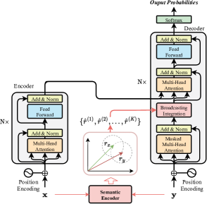
Figure 1: The framework of the CsaNMT.

2.1 Continuous Semantic Augmentation

We propose a novel data augmentation paradigm for neural machine translation, termed continuous semantic augmentation (CsaNMT), to better generalize the model’s capability to unseen instances. We adopt the Transformer (Vaswani et al., 2017) model as a backbone, and the framework is shown in Figure 1. In this architecture, an extra semantic encoder translates the source $\mathbf{x}$ and the target sentence $\mathbf{y}$ to real-value vectors $r_{x}=\psi(\mathbf{x};\Theta^{\prime})$ and $r_{y}=\psi(\mathbf{y};\Theta^{\prime})$ respectively, where $\psi(\cdot;\Theta^{\prime})$ is the forward function of the semantic encoder parameterized by $\Theta^{\prime}$ (parameters other than $\Theta$).

Definition 1.

There is a universal semantic space among the source and the target languages for neural machine translation, which is established by a semantic encoder. It defines a forward function $\psi(\cdot;\Theta^{\prime})$ to map discrete sentences into continuous vectors, that satisfies: $\forall(\mathbf{x},\mathbf{y})\in(\mathcal{X},\mathcal{Y}):r_{x}=r_{y}$. Besides, an adjacency semantic region $\nu(r_{x},r_{y})$ in the semantic space describes adequate variants of literal expression centered around each observed sentence pair $(\mathbf{x},\mathbf{y})$.

In our scenario, we first sample a series of vectors (denoted by $\mathcal{R}$) from the adjacency semantic region to augment the current training instance, that is $\mathcal{R}=\{\hat{r}^{(1)},\hat{r}^{(2)},...,\hat{r}^{(K)}\},\ {\rm where}\ \hat{r}^{(k)}\sim\nu(r_{x},r_{y})$. $K$ is the hyperparameter that determines the number of sampled vectors. Each sample $\hat{r}^{(k)}$ is then integrated into the generation process through a broadcasting integration network:

$$\hat{o}_{t}=W_{1}\hat{r}^{(k)}+W_{2}o_{t}+b,$$ (2)

where $o_{t}$ is the output of the self-attention module at position $t$. Finally, the training objective in Eq. (1) can be improved as

$$\begin{split}J_{mle}(\Theta)=&\mathbb{E}_{(\mathbf{x},\mathbf{y})\sim\mathcal{C},\hat{r}^{(k)}\in\mathcal{R}}\big{(}\log P(\mathbf{y}|\mathbf{x},\hat{r}^{(k)};\Theta)\big{)}\big{)}.\end{split}$$ (3)

By augmenting the training instance $(\mathbf{x},\mathbf{y})$ with diverse samples from the adjacency semantic region, the model is expected to generalize to more unseen instances. To this end, we must consider such two problems: (1) How to optimize the semantic encoder so that it produces a meaningful adjacency semantic region for each observed training pair. (2) How to obtain samples from the adjacency semantic region in an efficient and effective way. In the rest part of this section, we introduce the resolutions of these two problems, respectively.

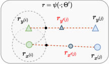
Figure 2: The diagram of formulating the adjacency semantic region for the sentence pair $(\mathbf{x}^{(i)},\mathbf{y}^{(i)})$.

Tangential Contrastive Learning

We start from analyzing the geometric interpretation of adjacency semantic regions. The schematic diagram is illustrated in Figure 2. Let $(\mathbf{x}^{(i)},\mathbf{y}^{(i)})$ and $(\mathbf{x}^{(j)},\mathbf{y}^{(j)})$ are two instances randomly sampled from the training corpora. For $(\mathbf{x}^{(i)},\mathbf{y}^{(i)})$, the adjacency semantic region $\nu(r_{x^{(i)}},r_{y^{(i)}})$ is defined as the union of two closed balls that are centered by $r_{x^{(i)}}$ and $r_{y^{(i)}}$, respectively. The radius of both balls is $d=\parallel r_{x^{(i)}}-r_{y^{(i)}}\parallel_{2}$, which is also considered as a slack variable for determining semantic equivalence. The underlying interpretation is that vectors whose distances from $r_{x^{(i)}}$ (or $r_{y^{(i)}}$) do not exceed $d$, are semantically-equivalent to both $r_{x^{(i)}}$ and $r_{y^{(i)}}$. To make $\nu(r_{x^{(i)}},r_{y^{(i)}})$ conform to the interpretation, we employ a similar method as in (Zheng et al., 2019; Wei et al., 2021) to optimize the semantic encoder with the tangential contrast.

Specifically, we construct negative samples by applying the convex interpolation between the current instance and other ones in the same training batch for instance comparison. And the tangent points (i.e., the points on the boundary) are considered as the critical states of semantic equivalence. The training objective is formulated as:

$$\begin{split}J_{ctl}(\Theta^{\prime})=&\mathbb{E}_{(\mathbf{x}^{(i)},\mathbf{y}^{(i)})\sim\mathcal{B}}\bigg{(}\log\frac{e^{s\big{(}r_{x^{(i)}},r_{y^{(i)}}\big{)}}}{e^{s\big{(}r_{x^{(i)}},r_{y^{(i)}}\big{)}}+\xi}\bigg{)},\\ \xi=&\sum_{j\&j\neq i}^{|\mathcal{B}|}\Big{(}e^{s\big{(}r_{y^{(i)}},r_{y^{\prime(j)}}\big{)}}+e^{s\big{(}r_{x^{(i)}},r_{x^{\prime(j)}}\big{)}}\Big{)},\end{split}$$ (4)

where $\mathcal{B}$ indicates a batch of sentence pairs randomly selected from the training corpora $\mathcal{C}$, and $s(\cdot)$ is the score function that computes the cosine similarity between two vectors. The negative samples $r_{x^{\prime(j)}}$ and $r_{y^{\prime(j)}}$ are designed as the following interpolation:

$$\begin{split}r_{x^{\prime(j)}}&=r_{x^{(i)}}+{\lambda}_{x}(r_{x^{(j)}}-r_{x^{(i)}}),{\lambda}_{x}\in(\frac{d}{d_{x}^{\prime}},1],\\ r_{y^{\prime(j)}}&=r_{y^{(i)}}+{\lambda}_{y}(r_{y^{(j)}}-r_{y^{(i)}}),{\lambda}_{y}\in(\frac{d}{d_{y}^{\prime}},1],\end{split}$$ (5)

where $d_{x}^{\prime}=\parallel r_{x^{(i)}}-r_{x^{(j)}}\parallel_{2}$ and $d_{y}^{\prime}=\parallel r_{y^{(i)}}-r_{y^{(j)}}\parallel_{2}$. The two equations in Eq. (5) set up when $d^{\prime}_{x}$ and $d^{\prime}_{y}$ are larger than $d$ respectively, or else $r_{x^{\prime(j)}}=r_{x^{(j)}}$ and $r_{y^{\prime(j)}}=r_{y^{(j)}}$. According to this design, an adjacency semantic region for the $i$-th training instance can be fully established by interpolating various instances in the same training batch. We follow Wei et al. (2021) to adaptively adjust the value of $\lambda_{x}$ (or $\lambda_{y}$) during the training process, and refer to the original paper for details.

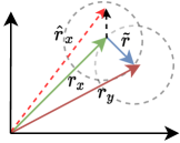
Figure 3: The geometric diagram of the proposed Mgrc sampling. $r_{x}$ and $r_{y}$ are the representations of the source sentence $\mathbf{x}$ and the target sentence $\mathbf{y}$, respectively. To construct the augmented sample, a straightforward idea is that: (1) transform the norm or the direction of $\tilde{r}=r_{y}-r_{x}$, formulated as $\omega\odot\tilde{r}$ (e.g., the black dashed arrow), in which each element $\omega_{i}\in[-1,1]$, and (2) combine $r_{x}$ (or $r_{y}$) and the transformation $\omega\odot\tilde{r}$ as $\hat{r}_{x}=r_{x}+\omega\odot\tilde{r}$ (i.e., the red dashed arrow).

Method	#Params.	Valid.	MT02	MT03	MT04	MT05	MT08	Avg.
Transformer, base (our implementation)	84M	45.09	45.63	45.07	46.59	45.84	36.18	43.86
Back-translation (Sennrich et al., 2016a)∗	84M	46.71	47.22	46.86	47.36	46.65	36.69	44.96
SwitchOut (Wang et al., 2018)∗	84M	46.13	46.72	45.69	47.08	46.19	36.47	44.43
SemAug (Wei et al., 2020a)	86M	-	-	-	49.15	49.21	40.94	-
AdvAug (Cheng et al., 2020)	-	49.26	49.03	47.96	48.86	49.88	39.63	47.07
CsaNMT, base	96M	50.46	49.65	48.84	49.80	50.40	41.63	48.06

Table 1: BLEU scores [%] on Zh$\rightarrow$En translation. “Params.” denotes the number of parameters (M=million). “$*$” indicates the results obtained by our implementation, we construct multiple pseudo sources for each target during back-translation but rather introducing extra monolingual corpora as in (Wei et al., 2020a) for fairer comparisons.

Mgrc Sampling

To obtain augmented data from the adjacency semantic region for the training instance $(\mathbf{x},\mathbf{y})$, we introduce a Mixed Gaussian Recurrent Chain (denoted by Mgrc) algorithm to design an efficient and effective sampling strategy. As illustrated in Figure 3, we first transform the bias vector $\tilde{r}=r_{y}-r_{x}$ according to a pre-defined scale vector $\omega$, that is $\omega\odot\tilde{r}$, where $\odot$ is the element-wise product operation. Then, we construct a novel sample $\hat{r}=r+\omega\odot\tilde{r}$ for augmenting the current instance, in which $r$ is either $r_{x}$ or $r_{y}$. As a consequence, the goal of the sampling strategy turns into find a set of scale vectors, i.e. $\omega\in\{\omega^{(1)},\omega^{(2)},...,\omega^{(K)}\}$. Intuitively, we can assume that $\omega$ follows a distribution with universal or Gaussian forms, despite the latter demonstrates better results in our experience. Formally, we design a mixed Gaussian distribution as follow:

$$\begin{split}\omega^{(k)}&\sim p(\omega|\omega^{(1)},\omega^{(2)},...,\omega^{(k-1)}),\\ p&=\eta\mathcal{N}\big{(}\mathbf{0},{\rm diag}(\mathcal{W}_{r}^{2})\big{)}\\ &+(1.0-\eta)\mathcal{N}\bigg{(}\frac{1}{k-1}\sum_{i=1}^{k-1}\omega^{(i)},\mathbf{1}\bigg{)}.\end{split}$$ (6)

This framework unifies the recurrent chain and the rejection sampling mechanism. Concretely, we first normalize the importance of each dimension in $\tilde{r}$ as ${\mathcal{W}_{r}=\frac{|\tilde{r}|-min(|\tilde{r}|)}{max(|\tilde{r}|)-min(|\tilde{r}|)}}$, the operation $|\cdot|$ takes the absolute value of each element in the vector, which means the larger the value of an element is the more informative it is. Thus $\mathcal{N}(\mathbf{0},{\rm diag}(\mathcal{W}_{r}^{2}))$ limits the range of sampling to a subspace of the adjacency semantic region, and rejects to conduct sampling from the uninformative dimensions. Moreover, $\mathcal{N}(\frac{1}{k-1}\sum_{i=1}^{k-1}\omega^{(i)},\mathbf{1})$ simulates a recurrent chain that generates a sequence of reasonable vectors where the current one is dependent on the prior vectors. The reason for this design is that we expect that $p$ in Eq. (6) can become a stationary distribution with the increase of the number of samples, which describes the fact that the diversity of each training instance is not infinite. $\eta$ is a hyper-parameter to balance the importance of the above two Gaussian forms. For a clearer presentation, Algorithm 1 summarizes the sampling process.

Algorithm 1 Mgrc Sampling

0:  The representations of the training instance $(\mathbf{x},\mathbf{y})$, i.e. $r_{x}$ and $r_{y}$.

0:  A set of augmented samples $\mathcal{R}=\{\hat{r}^{(1)},\hat{r}^{(2)},...,\hat{r}^{(K)}\}$

1:  Normalizing the importance of each element in $\tilde{r}=r_{y}-r_{x}$: ${\mathcal{W}_{r}=\frac{|\tilde{r}|-min(|\tilde{r}|)}{max(|\tilde{r}|)-min(|\tilde{r}|)}}$

2:  Set $k=1$, $\omega^{(1)}\sim\mathcal{N}(\mathbf{0},{\rm diag}(\mathcal{W}_{r}^{2}))$, $\hat{r}^{(1)}=r+\omega^{(1)}\odot(r_{y}-r_{x})$

3:  Initialize the set of samples as $\mathcal{R}=\{\hat{r}^{(1)}\}$.

4:  while $k\leq(K-1)$ do

5:     $k\leftarrow k+1$

6:     Calculate the current scale vector: $\omega^{(k)}\sim p(\omega|\omega^{(1)},\omega^{(2)},...,\omega^{(k-1)}$ according to Eq. (6).

7:     Calculate the current sample: $\hat{r}^{(k)}=r+\omega^{(k)}\odot(r_{y}-r_{x})$.

8:     $\mathcal{R}\leftarrow\mathcal{R}\bigcup\{\hat{r}^{(k)}\}$.

9:  end while

2.2 Training and Inference

The training objective in our approach is a combination of $J_{mle}(\Theta)$ in Eq. (3) and $J_{ctl}(\Theta^{\prime})$ in Eq. (4). In practice, we introduce a two-phase training procedure with mini-batch losses. Firstly, we train the semantic encoder from scratch using the task-specific data, i.e. $\Theta^{\prime*}=\operatorname*{argmax}_{\Theta^{\prime}}J_{ctl}(\Theta^{\prime})$. Secondly, we optimize the encoder-decoder model by maximizing the log-likelihood, i.e. $\Theta^{*}=\operatorname*{argmax}_{\Theta}J_{mle}(\Theta)$, and fine-tune the semantic encoder with a small learning rate at the same time.

During inference, the sequence of target words is generated auto-regressively, which is almost the same as the vanilla Transformer (Vaswani et al., 2017). A major difference is that our method involves the semantic vector of the input sequence for generation: $y_{t}^{*}=\operatorname*{argmax}_{y_{t}}P(\cdot|\mathbf{y}_{<t},\mathbf{x},r_{x};\Theta)$, where $r_{x}=\psi(\mathbf{x};\Theta^{\prime})$. This module is plug-in-use as well as is agnostic to model architectures.

Model	WMT 2014 En$\rightarrow$De			WMT 2014 En$\rightarrow$Fr
	#Params.	BLEU	SacreBLEU	#Params.	BLEU	SacreBLEU
Transformer, base (our implementation)	62M	27.67	26.8	67M	40.53	38.5
Transformer, big (our implementation)	213M	28.79	27.7	222M	42.36	40.3
Back-Translation (Sennrich et al., 2016a)∗	213M	29.25	28.2	222M	41.73	39.7
SwitchOut (Wang et al., 2018)∗	213M	29.18	28.1	222M	41.62	39.6
SemAug (Wei et al., 2020a)	221M	30.29	-	230M	42.92	-
AdvAug (Cheng et al., 2020)	†65M	29.57	-	-	-	-
Data Diversification (Nguyen et al., 2020)	†1260M	30.70	-	†1332M	43.70	-
CsaNMT, base	74M	30.16	29.2	80M	42.40	40.3
CsaNMT, big	265M	30.94	29.8	274M	43.68	41.6

Table 2: BLEU scores [%] on the WMT14 En$\rightarrow$De and En$\rightarrow$Fr tasks. “$*$” indicates the results obtained by our implementation, which is the same in Table 1. “^†” denote estimate values. We further compare against the baselines with increased amounts of parameters, and investigate the performance of CsaNMT equipped with much stronger baselines (e.g. deep and scale Transformers (Ott et al., 2018; Wang et al., 2019; Wei et al., 2020b)) in Sec. 3.3.

3 Experiments

We first apply CsaNMT to NIST Chinese-English (Zh$\rightarrow$En), WMT14 English-German (En$\rightarrow$De) and English-French (En$\rightarrow$Fr) tasks, and conduct extensive analyses for better understanding the proposed method. And then we generalize the capability of our method to low-resource IWSLT tasks.

3.1 Settings

Datasets. For the Zh$\rightarrow$En task, the LDC corpus is taken into consideration, which consists of 1.25M sentence pairs with 27.9M Chinese words and 34.5M English words, respectively. The NIST 2006 dataset is used as the validation set for selecting the best model, and NIST 2002 (MT02), 2003 (MT03), 2004 (MT04), 2005 (MT05), 2008 (MT08) are used as the test sets. For the En$\rightarrow$De task, we employ the popular WMT14 dataset, which consists of approximately 4.5M sentence pairs for training. We select newstest2013 as the validation set and newstest2014 as the test set. For the En$\rightarrow$Fr task, we use the significantly larger WMT14 dataset consisting of 36M sentence pairs. The combination of {newstest2012, 2013} was used for model selection and the experimental results were reported on newstest2014. Refer to Appendix A for more details.

Training Details. We implement our approach on top of the Transformer (Vaswani et al., 2017). The semantic encoder is a 4-layer transformer encoder with the same hidden size as the backbone model. Following sentence-bert (Reimers and Gurevych, 2019), we average the outputs of all positions as the sequence-level representation. The learning rate for finetuning the semantic encoder at the second training stage is set as $1e-5$. All experiments are performed on 8 V100 GPUs. We accumulate the gradient of 8 iterations and update the models with a batch of about 65K tokens. The hyperparameters $K$ and $\eta$ in Mgrc sampling are tuned on the validation set with the range of $K\in\{10,20,40,80\}$ and $\eta\in\{0.15,0.30,0.45,0.6,0.75,0.90\}$. We use the default setup of $K=40$ for all three tasks, $\eta=0.6$ for both Zh$\rightarrow$En and En$\rightarrow$De while $\eta=0.45$ for En$\rightarrow$Fr. For evaluation, the beam size and length penalty are set to 4 and 0.6 for the En$\rightarrow$De as well as En$\rightarrow$Fr, while 5 and 1.0 for the Zh$\rightarrow$En task.

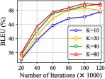
(a) NIST Zh$\rightarrow$En

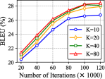
(b) WMT14 En$\rightarrow$De

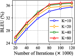
(c) WMT14 En$\rightarrow$Fr

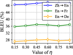
(d) Effect of $\eta$.

Figure 4: Effects of $K$ and $\eta$ on validation sets. (a), (b) and (c) depict the BLEU curves with different values of $K$ on Zh$\rightarrow$En, En$\rightarrow$De and En$\rightarrow$Fr, respectively. (d) demonstrates the performances of $\eta$ with different values.

3.2 Main Results

Results of Zh$\rightarrow$En. Table 1 shows the results on the Chinese-to-English translation task. From the results, we can conclude that our approach outperforms existing augmentation strategies such as back-translation (Sennrich et al., 2016a; Wei et al., 2020a) and switchout (Wang et al., 2018) by a large margin (up to 3.63 BLEU), which verifies that augmentation in continuous space is more effective than methods with discrete manipulations. Compared to the approaches that replace words in the embedding space (Cheng et al., 2020), our approach also demonstrates superior performance, which reveals that sentence-level augmentation with continuous semantics works better on generalizing to unseen instances. Moreover, compared to the vanilla Transformer, our approach consistently achieves promising improvements on five test sets.

Results of En$\rightarrow$De and En$\rightarrow$Fr. From Table 2, our approach consistently performs better than existing methods (Sennrich et al., 2016a; Wang et al., 2018; Wei et al., 2020a; Cheng et al., 2020), yielding significant gains (0.65$\sim$1.76 BLEU) on the En$\rightarrow$De and En$\rightarrow$Fr tasks. An exception is that Nguyen et al. (2020) achieved comparable results with ours via multiple forward and backward NMT models, thus data diversification intuitively demonstrates lower training efficiency. Moreover, we observe that CsaNMT gives 30.16 BLEU on the En$\rightarrow$De task with the base setting, significantly outperforming the vanilla Transformer by 2.49 BLEU points. Our approach yields a further improvement of 0.68 BLEU by equipped with the wider architecture, demonstrating superiority over the standard Transformer by 2.15 BLEU. Similar observations can be drawn for the En$\rightarrow$Fr task.

3.3 Analysis

Effects of $K$ and $\eta$. Figure 4 illustrates how the hyper-parameters $K$ and $\eta$ in Mgrc sampling affect the translation quality. From Figures 4(a)-4(c), we can observe that gradually increasing the number of samples significantly improves BLEU scores, which demonstrates large gaps between $K=10$ and $K=40$. However, assigning larger values (e.g., $80$) to $K$ does not result in further improvements among all three tasks. We conjecture that the reasons are two folds: (1) it is fact that the diversity of each training instance is not infinite and thus Mgrc gets saturated is inevitable with $K$ increasing. (2) Mgrc sampling with a scaled item (i.e., $\mathcal{W}_{r}$) may degenerate to traverse in the same place. This prompts us to design more sophisticated algorithms in future work. In our experiments, we default set $K=40$ to achieve a balance between the training efficiency and translation quality. Figure 4(d) shows the effect of $\eta$ on validation sets, which balances the importance of two Gaussian forms during the sampling process. The setting of $\eta=0.6$ achieves the best results on both the Zh$\rightarrow$En and En$\rightarrow$De tasks, and $\eta=0.45$ consistently outperforms other values on the En$\rightarrow$Fr task.

Lexical diversity and semantic faithfulness. We demonstrate both the lexical diversity (measured by TTR$=\frac{num.\ of\ types}{num.\ of\ tokens}$) of various translations and the semantic faithfulness of machine translated ones (measured by BLEURT with considering human translations as the references) in Table 4. It is clear that CsaNMT substantially bridge the gap of the lexical diversity between translations produced by human and machine. Meanwhile, CsaNMT shows a better capability on preserving the semantics of the generated translations than Transformer. We intuitively attribute the significantly increases of BLEU scores on all datasets to these two factors. We also have studied the robustness of CsaNMT towards noisy inputs and the translationese effect, see Appendix D for details.

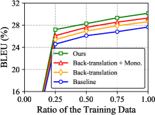
Figure 5: Comparison between discrete and continuous augmentations with different ratios of the training data.

Model	BLEU	Dec. speed
Transformer-base	27.67	reference
Default 4-layer semantic encoder	30.16	0.95$\times$
Remove the extra semantic encoder	28.71	1.0$\times$
Take PTMs as the semantic encoder	31.10	0.62$\times$

Table 3: Effect of the semantic encoder variants.

	TTR			BLEURT Score
	Zh	De	Fr	Zh	De	Fr
Human	7.58%	22.08%	13.98%	-	-	-
Trans.	6.95%	20.32%	11.76%	0.570	0.635	0.696
CsaNMT	7.13%	21.26%	12.91%	0.581	0.684	0.739

Table 4: TTR (Type-Token-Ratio) (Templin, 1957) and BLEURT scores of Zh$\rightarrow$En and En$\rightarrow$X translations produced by Human, vanilla Transformer (written as Trans.), and CsaNMT. “Human” translations mean the references contained in the standard test sets. Refer to Appendix D for the results on robustness test sets.

#	Objective	Sampling	BLEU
1	Default tangential CTL	Default Mgrc	30.16
2	Default tangential CTL	Mgrc w/o recurrent chain	29.64
3	Default tangential CTL	Mgrc w/ uniform dist.	29.78
4	Variational Inference	Gaussian sampling	28.07
5	Cosine similarity	Default Mgrc	28.19

Table 5: Effect of Mgrc sampling and tangential contrastive learning on En$\rightarrow$De validation set.

Effect of the semantic encoder. We introduce two variants of the semantic encoder to investigate its performance on En$\rightarrow$De validation set. Specifically, (1) we remove the extra semantic encoder and construct the sentence-level representations by averaging the sequence of outputs of the vanilla sentence encoder. (2) We replace the default 4-layer semantic encoder with a large pre-trained model (PTM) (i.e., XLM-R Conneau et al. (2020)). The results are reported in Table 3. Comparing line 2 with line 3, we can conclude that an extra semantic encoder is necessary for constructing the universal continuous space among different languages. Moreover, when the large PTM is incorporated, our approach yields further improvements, but it causes massive computational overhead.

Comparison between discrete and continuous augmentations. To conduct detailed comparisons between different augmentation methods, we asymptotically increase the training data to analyze the performance of them on the En$\rightarrow$De translation. As in Figure 5, our approach significantly outperforms the back-translation method on each subset, whether or not extra monolingual data Sennrich et al. (2016a) is introduced. These results demonstrate the stronger ability of our approach than discrete augmentation methods on generalizing to unseen instances with the same set of observed data points. Encouragingly, our approach achieves comparable performance with the baseline model with only 25% of training data, which indicates that our approach has great potential to achieve good results with very few data.

Effect of Mgrc sampling and tangential contrastive learning. To better understand the effectiveness of the Mgrc sampling and the tangential contrastive learning, we conduct detailed ablation studies in Table 5. The details of four variants with different objectives or sampling strategies are shown in Appendix C. From the results, we can observe that both removing the recurrent dependence and replacing the Gaussian forms with uniform distributions make the translation quality decline, but the former demonstrates more drops. We also have tried the training objectives with other forms, such as variational inference and cosine similarity, to optimize the semantic encoder. However, the BLEU score drops significantly.

Training Cost and Convergence. Figure 6 shows the evolution of BLEU scores during training. It is obvious that our method performs consistently better than both the vanilla Transformer and the back-translation method at each iteration (except for the first 10K warm-up iterations, where the former one has access to less unique training data than the latter two due to the $K$ times over-sampling). For the vanilla Transformer, the BLEU score reaches its peak at about 52K iterations. In comparison, both CsaNMT and the back-translation method require 75K updates for convergence. In other words, CsaNMT spends 44% more training costs than the vanilla Transformer, due to the longer time to make the NMT model converge with augmented training instances. This is the same as the back-translation method.

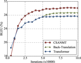
Figure 6: BLEU curves over iterations on the WMT14 English$\rightarrow$German test set. Note that back-translation is initialized from the vanilla Transformer.

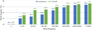
Figure 7: Comparison between the vanilla Transformer and CsaNMT on prediction accuracy of words with different frequencies.

Word prediction accuracy. Figure 7 illustrates the prediction accuracy of both frequent and rare words. As expected, CsaNMT generalizes to rare words better than the vanilla Transformer, and the gap of word prediction accuracy is as large as 16%. This indicates that the NMT model alleviates the probability under-estimation of rare words via continuous semantic augmentation.

Effects of Additional Parameters and Strong Baselines. In contrast to the vanilla Transformer, CsaNMT involves with approximate 20% additional parameters. In this section, we further compare against the baselines with increased amounts of parameters, and investigate the performance of CsaNMT equipped with much stronger baselines (e.g. deep and scale Transformers (Ott et al., 2018; Wang et al., 2019; Wei et al., 2020b)). From the results on WMT14 testsets in Table 6, we can observe that CsaNMT still outperforms the vanilla Transformer (by more than 1.2 BLEU) under the same amount of parameters, which shows that the additional parameters are not the key to the improvement. Moreover, CsaNMT yields at least 0.9 BLEU gains equipped with much stronger baselines. For example, the scale Transformer (Ott et al., 2018), which originally gives 29.3 BLEU in the En$\rightarrow$De task, now gives 31.37 BLEU with our continuous semantic augmentation strategy. It is important to mention that our method can help models to achieve further improvement, even if they are strong enough.

Model	#Params.	En$\rightarrow$De	En$\rightarrow$Fr
Transformer (Vaswani et al., 2017)†	213M	28.40	41.80
Transformer (our impl.)	213M	28.79	42.36
Transformer (our impl., 10 layers)	265M	29.08	42.49
CsaNMT	265M	30.94	43.68
Scale Trans. (Ott et al., 2018)†	210M	29.30	43.20
Deep (Wang et al., 2019)	350M	30.26	43.24
Msc (Wei et al., 2020b)†	512M	30.56	-
Our CsaNMT with
Scale Trans. (Ott et al., 2018)	263M	31.37	44.12
Deep (Wang et al., 2019)	405M	31.35	-
Msc (Wei et al., 2020b)	566M	31.49	-

Table 6: BLEU scores [%] on WMT14 testsets for the English-German (En$\rightarrow$De) and English-French (En$\rightarrow$Fr) tasks. Superscript ^† denotes the numbers are reported from the paper, others are based on our runs. “-” means omitted results because of the limitations of GPU resources. “10 layers” means that we construct the Transformer with a 10-layer encoder, thus it has the same amount of parameters as our model.

3.4 Low-Resource Machine Translation

Model	English-German	English-French
Transformer	28.64	35.8
Back-translation	29.45	36.3
CsaNMT	31.29	38.6

Table 7: BLEU scores [%] on the IWSLT tasks. For fairer comparison, all the models are implemented by ourselves using the same backbone, and the extra monolingual corpora is not introduced into back-translation.

We further generalize the capability of the proposed CsaNMT to various low-resource machine translation tasks, including IWSLT14 English-German and IWSLT17 English-French. The details of the datasets and model configurations can be found in Appendix B. Table 7 shows the results of different models. Compared to the vanilla Transformer, the proposed CsaNMT improve the BLEU scores of the two tasks by 2.7 and 2.9 points, respectively. This result indicates that the claiming of the continuous semantic augmentation enriching the training corpora with very limited observed instances.

4 Related Work

Data Augmentation (DA) Edunov et al. (2018); Kobayashi (2018); Gao et al. (2019); Khayrallah et al. (2020); Pham et al. (2021) has been widely used in neural machine translation. The most popular one is the family of back-translation Sennrich et al. (2016a); Nguyen et al. (2020), which utilizes a target-to-source model to translate monolingual target sentences back into the source language. Besides, constructing adversarial training instances with diverse literal forms via word replacing or embedding interpolating (Wang et al., 2018; Cheng et al., 2020) is beneficial to improve the generalization performance of NMT models.

Vicinal Risk Minimization (VRM) (Chapelle et al., 2000) is another principle of data augmentation, in which DA is formalized as extracting additional pseudo samples from the vicinal distribution of observed instances. Typically the vicinity of each training instance is defined artificially according to the characteristics of the dataset (or task), such as color (scale, mixup) augmentation (Simonyan and Zisserman, 2014; Krizhevsky et al., 2012; Zhang et al., 2018) in computer vision and adversarial augmentation with manifold neighborhoods (Ng et al., 2020; Cheng et al., 2021) in NLP. Our approach relates to VRM that involves with an adjacency semantic region as the vicinity manifold for each training instance.

Sentence Representation Learning is a well investigated area with dozens of methods (Kiros et al., 2015; Cer et al., 2018; Yang et al., 2018). In recent years, the methods built on large pre-trained models (Devlin et al., 2019; Conneau et al., 2020) have been widely used for learning sentence level representations (Reimers and Gurevych, 2019; Huang et al., 2019; Yang et al., 2019). Our work is also related to the methods that aims at learning the universal representation Zhang et al. (2016); Schwenk and Douze (2017); Yang et al. (2021) for multiple semantically-equivalent sentences in NMT. In this context, contrastive learning has become a popular paradigm in NLP (Kong et al., 2020; Clark et al., 2020; Gao et al., 2021). The most related work are Wei et al. (2021) and Chi et al. (2021), which suggested transforming cross-lingual sentences into a shared vector by contrastive objectives.

5 Conclusion

We propose a novel data augmentation paradigm CsaNMT, which involves with an adjacency semantic region as the vicinity manifold for each training instance. This method is expected to make more unseen instances under generalization with very limited training data. The main components of CsaNMT consists of the tangential contrastive learning and the Mixed Gaussian Recurrent Chain (Mgrc) sampling. Experiments on both rich- and low-resource machine translation tasks demonstrate the effectiveness of our method.

In the future work, we would like to further study the vicinal risk minimization with the combination of multi-lingual aligned scenarios and large-scale monolingual data, and development it as a pure data augmentator merged into the vanilla Transformer.

Appendix A Details of Rich-Resource Datasets

Variants	Training Objective for the Semantic Encoder	Sampling Strategy for Obtaining Augmented Samples
1	$\mathbb{E}_{(\mathbf{x}^{(i)},\mathbf{y}^{(i)})\sim\mathcal{B}}\Bigg{(}\log\frac{e^{s\big{(}r_{x^{(i)}},r_{y^{(i)}}\big{)}}}{e^{s\big{(}r_{x^{(i)}},r_{y^{(i)}}\big{)}}+\sum_{j\&j\neq i}^{|\mathcal{B}|}\Big{(}e^{s\big{(}r_{y^{(i)}},r_{y^{\prime(j)}}\big{)}}+e^{s\big{(}r_{x^{(i)}},r_{x^{\prime(j)}}\big{)}}\Big{)}}\Bigg{)}$	$\omega^{(k)}\sim\eta\mathcal{N}\big{(}\mathbf{0},{\rm diag}(\mathcal{W}_{r}^{2})\big{)}+(1.0-\eta)\mathcal{N}\big{(}\mathbf{0},\mathbf{1}\big{)}$
2	ditto	$\omega^{(k)}\sim\eta\mathcal{U}\big{(}-\mathcal{W}_{r},\mathcal{W}_{r}\big{)}+(1.0-\eta)\mathcal{U}\big{(}\bar{\mathbf{a}}-\mathbf{1},\mathbf{1}-\bar{\mathbf{a}}\big{)}$
		where $\bar{\mathbf{a}}=\frac{1}{k-1}\sum_{i=1}^{k-1}\omega^{(i)}$
3	$\mathbb{E}_{(\mathbf{x}^{(i)},\mathbf{y}^{(i)})\sim\mathcal{B}}\Big{(}-KL\big{(}p(r_{x^{(i)}})\parallel q(r_{x^{(i)}},r_{y^{(i)}})\big{)}\Big{)}$	$\hat{r}_{x}=\mu+\epsilon\odot\sigma$
	where $p(r_{x^{(i)}})\sim\mathcal{N}(\mu,\sigma^{2})$ and $q(r_{x^{(i)}},r_{y^{(i)}})\sim\mathcal{N}(\mu^{\prime},\sigma^{\prime 2})$	where $\epsilon$ is a standard Gaussian noise
4	$\mathbb{E}_{(\mathbf{x}^{(i)},\mathbf{y}^{(i)})\sim\mathcal{B}}\Big{(}\frac{r_{x^{(i)}}^{T}r_{y^{(i)}}}{\parallel r_{x^{(i)}}\parallel\cdot\parallel r_{y^{(i)}}\parallel}\Big{)}$	$\omega^{(k)}\sim\eta\mathcal{N}\big{(}\mathbf{0},{\rm diag}(\mathcal{W}_{r}^{2})\big{)}+(1.0-\eta)\mathcal{N}\Big{(}\frac{1}{k-1}\sum_{i=1}^{k-1}\omega^{(i)},\mathbf{1}\Big{)}$

Table 8: The variants of the training objective for the semantic encoder as well as the sampling strategy for obtaining augmented samples.

Model	Noisy Inputs				Translationese
	Original	WS	WD	WR	${\bf X\rightarrow Y^{*}}$	${\bf X^{*}\rightarrow Y}$	${\bf X^{**}\rightarrow Y^{*}}$
Transformer (our implementation)	27.67	15.33	18.59	16.98	32.82	28.56	39.04
Back-Translation (our implementation)	29.25	17.20	20.44	18.71	33.07	29.73	39.86
CsaNMT	30.16	20.14	23.76	21.66	34.62	30.70	41.64

Table 9: BLEU scores [%] on noisy inputs and the translationese effect, in the WMT14 En$\rightarrow$De setup.

For the Zh$\rightarrow$En task, the LDC corpus is taken into consideration, which consists of 1.25M sentence pairs with 27.9M Chinese words and 34.5M English words, respectively. The NIST 2006 dataset is used as the validation set for selecting the best model, and NIST 2002 (MT02), 2003 (MT03), 2004 (MT04), 2005 (MT05), 2008 (MT08) are used as the test sets. We created shared BPE (byte-pair-encoding (Sennrich et al., 2016b)) codes with 60K merge operations to build two vocabularies comprising 47K Chinese sub-words and 30K English sub-words. For the En$\rightarrow$De task, we employ the popular WMT14 dataset, which consists of approximately 4.5M sentence pairs for training. We select newstest2013 as the validation set and newstest2014 as the test set. All sentences had been jointly byte-pair-encoded with 32K merge operations, which results in a shared source-target vocabulary of about 37K tokens. For the En$\rightarrow$Fr task, we use the significantly larger WMT14 dataset consisting of 36M sentence pairs. The combination of {newstest2012, 2013} was used for model selection and the experimental results were reported on newstest2014.

We use the Stanford segmenter (Tseng et al., 2005) for Chinese word segmentation and apply the script tokenizer.pl of Moses (Koehn et al., 2007) for English, German and French tokenization. We measure the performance with the 4-gram BLEU score (Papineni et al., 2002). Both the case-sensitive tokenized BLEU (compued by multi-bleu.pl) and the detokenized sacrebleu (Post, 2018) are reported on the En$\rightarrow$De and En$\rightarrow$Fr tasks. The case-insensitive BLEU is reported on the Zh$\rightarrow$En task.

Appendix B Low-Resource Machine Translation

Datasets.

For IWSLT14 En$\rightarrow$De, there are $160k$ sentence pairs for training and $7584$ sentence pairs for validation. As in previous work Ranzato et al. (2016); Zhu et al. (2020), the concatenation of dev2010, dev2012, test2010, test2011 and test2012 is used as the test set. For IWSLT17 En$\rightarrow$Fr, there are $236k$ sentence pairs for training and $10263$ for validation. The concatenation of test2010, test2011, test2012, test2013, test2014 and test2015 is used as the test set. We use a joint source and target vocabulary with $10k$ byte-pair-encoding (BPE) types Sennrich et al. (2016b) for above two tasks.

Model Settings.

The model configuration is transformer_iwslt, representing a 6-layer model with embedding size 512 and FFN layer dimension 1024. We train all models using the Adam optimizer with adaptive learning rate schedule (warm-up step with 4K) as in Vaswani et al. (2017). During inference, we use beam search with a beam size of $5$ and length penalty of $1.0$.

Appendix C Variants with Different Objectives or Sampling Strategies

Table 8 describes the details of four variants (introduced in Table 5, from row 2 to row 5) with different objectives or sampling strategies: (1) default tangential CTL in Eq. (4) + Mgrc w/o recurrent dependence, (2) default tangential CTL in Eq. (4) + Mgrc w uniform distribution, (3) variational inference (Zhang et al., 2016) + Gaussian sampling, and (4) cosine similarity + default Mgrc sampling.

Appendix D Robustness on Noisy Inputs and Translationese

In this section, we study the robustness of our CsaNMT towards both noisy inputs and the translationese effect (Volansky et al., 2013) on newstest2014 for the WMT14 English-German task.

Noisy Inputs.

Inspired by (Gao et al., 2019), we construct noisy test sets via several strategies described as follows:

• Original: the original testset without any manipulations;

• WS: word swap, randomly swap words in nearby positions within a window size 3 (Artetxe et al., 2018; Lample et al., 2018b);

• WD: word dropout, randomly drop words with a ratio of 15% (Iyyer et al., 2015; Lample et al., 2018b);

• WR: word replace, randomly replace word tokens with a placeholder token (e.g., [UNK]) (Xie et al., 2017) or with a relevant (measured by the similarity of word embeddings) alternative (Cheng et al., 2019). The replacement ratio also is 15%.

Translationese Effect.

Edunov et al. (2020) pointed out that “back-translation (BT) suffers from the translationese effect. That is BT only shows significant improvements for test examples where the source itself is a translation, or translationese, while is ineffective to translate natural text”. To test the effect of our method on translationese, we follow the same settings and testsets provided by Edunov et al. (2020):

• natural source $\rightarrow$ translationese target (${\bf X\rightarrow Y^{*}}$);

• translationese source $\rightarrow$ natural target (${\bf X^{*}\rightarrow Y}$);

• round-trip translationese source $\rightarrow$ translationese target (${\bf X^{**}\rightarrow Y^{*}}$), where ${\bf X\rightarrow Y^{*}\rightarrow X^{**}}$.

Results.

As shown in Table 9, our approach shows better robustness over two baseline methods across various artificial noises. Moreover, CsaNMT consistently outperforms the baseline in all three translationese scenarios, the same is true for back-translation. However, Edunov et al. (2020) shows that BT improves only in the ${\bf X^{*}\rightarrow Y}$ scenario. Our explanation for the inconsistency is that BT without monolingual data in our setting benefits from the natural parallel data to deal with the translationese sources.

Appendix E Codes of tangential contrastive learning and Mgrc sampling

E.1 Tangential Contrastive Learning

⬇

# src_embedding: [batch_size, 1, hidden_size]

# trg_embedding: [batch_size, 1, hidden_size]

def get_ctl_loss(src_embedding, trg_embedding, dynamic_coefficient):

batch_size = tf.shape(src_embedding)[0]

def get_ctl_logits(query, keys):

# expand_query: [batch_size, batch_size, hidden_size]

# expand_keys: [batch_size, batch_size, hidden_size]

# the current ref is the positive key, while others in the training batch are negative ones

expand_query = tf.tile(query, [1, batch_size, 1])

expand_keys = tf.tile(tf.transpose(keys, [1,0,2]), [batch_size, 1, 1])

# distances between queries and positive keys

d_pos = tf.sqrt(tf.reduce_sum(tf.pow(query - keys, 2.0), axis=-1)) # [batch_size, 1]

d_pos = tf.tile(d_pos, [1, batch_size]) # [batch_size, batch_size]

d_neg = tf.sqrt(tf.reduce_sum(tf.pow(expand_query - expand_keys, 2.0), axis=-1)) # [batch_size, batch_size]

lambda_coefficient = (d_pos / d_neg) ** dynamic_coefficient

hardness_masks = tf.cast(tf.greater(d_neg, d_pos), dtype=tf.float32)

hard_keys =(expand_query + tf.expand_dims(lambda_coefficient, axis=2) * (expand_keys - expand_query)) * \

tf.expand_dims(hardness_masks, axis=2) + expand_keys * tf.expand_dims(1.0 - hardness_masks, axis=2)

logits = tf.matmul(query, hard_keys, transpose_b=True) # [batch_size, 1, batch_size]

return logits

logits_src_trg = get_ctl_logits(src_embedding, trg_embedding)

logits_trg_src = get_ctl_logits(trg_embedding, src_embedding) + tf.expand_dims(tf.matrix_band_part(tf.ones([batch_size, batch_size]), 0, 0) * -1e9, axis=1)

logits = tf.concat([logits_src_trg, logits_trg_src], axis=2) # [batch_size, 1, 2*batch_size]

labels = tf.expand_dims(tf.range(batch_size, dtype=tf.int32), axis=1)

labels = tf.one_hot(labels, depth=2*batch_size, on_value=1.0, off_value=0.0)

cross_entropy_fn = tf.nn.softmax_cross_entropy_with_logits

loss = tf.reduce_mean(cross_entropy_fn(logits=logits, labels=labels))

return loss

E.2 Mgrc Sampling

⬇

# src_embedding: [batch_size, hidden_size]

# trg_embedding: [batch_size, hidden_size]

# default: K=20 and eta = 0.6

def mgrc_sampling(src_embedding, trg_embedding, K, eta):

batch_size = tf.shape(src_embedding)[0]

def get_samples(x_vector, y_vector):

bias_vector = y_vector - x_vector

W_r = (tf.abs(bias_vector) - tf.reduce_min(tf.abs(bias_vector), axis=1, keep_dims=True)) / \

(tf.reduce_max(tf.abs(bias_vector), 1, keep_dims=True) - tf.reduce_min(tf.abs(bias_vector), 1, keep_dims=True))

# initializing the set of samples

R = []

omega = tf.random_normal(tf.shape(bias_vector), 0, W_r)

sample = x_vector + tf.multiply(omega, bias_vector)

R.append(sample)

for i in xrange(1, K):

chain = [tf.expand_dims(item, axis=1) for item in R[:i]]

average_omega = tf.reduce_mean(tf.concat(chain, axis=1), axis=1)

omega = eta * tf.random_normal(tf.shape(bias_vector), 0, W_r) + \

(1.0 - eta) * tf.random_normal(tf.shape(bias_vector), average_omega, 1.0)

sample = x_vector + tf.multiply(omega, bias_vector)

R.append(sample)

return R

x_sample = get_samples(src_embedding, trg_embedding)

y_sample = get_samples(trg_embedding, src_embedding)

return x_sample.extend(y_sample)

References

- Artetxe et al. (2018) Mikel Artetxe, Gorka Labaka, Eneko Agirre, and Kyunghyun Cho. 2018. Unsupervised neural machine translation. In International Conference on Learning Representations.
- Cer et al. (2018) Daniel Cer, Yinfei Yang, Sheng-yi Kong, Nan Hua, Nicole Limtiaco, Rhomni St. John, Noah Constant, Mario Guajardo-Cespedes, Steve Yuan, Chris Tar, Yun-Hsuan Sung, Brian Strope, and Ray Kurzweil. 2018. Universal sentence encoder. CoRR, abs/1803.11175.
- Chapelle et al. (2000) Olivier Chapelle, Jason Weston, Léon Bottou, and Vladimir Vapnik. 2000. Vicinal risk minimization. In Advances in Neural Information Processing Systems, volume 13. MIT Press.
- Cheng et al. (2019) Yong Cheng, Lu Jiang, and Wolfgang Macherey. 2019. Robust neural machine translation with doubly adversarial inputs. In Proceedings of the 57th Annual Meeting of the Association for Computational Linguistics, pages 4324–4333. Association for Computational Linguistics.
- Cheng et al. (2020) Yong Cheng, Lu Jiang, Wolfgang Macherey, and Jacob Eisenstein. 2020. AdvAug: Robust adversarial augmentation for neural machine translation. In Proceedings of the 58th Annual Meeting of the Association for Computational Linguistics, pages 5961–5970. Association for Computational Linguistics.
- Cheng et al. (2018) Yong Cheng, Zhaopeng Tu, Fandong Meng, Junjie Zhai, and Yang Liu. 2018. Towards robust neural machine translation. In Proceedings of the 56th Annual Meeting of the Association for Computational Linguistics (Volume 1: Long Papers), pages 1756–1766. Association for Computational Linguistics.
- Cheng et al. (2021) Yong Cheng, Wei Wang, Lu Jiang, and Wolfgang Macherey. 2021. Self-supervised and supervised joint training for resource-rich machine translation. In International Conference on Machine Learning, pages 1825–1835. PMLR.
- Cheng et al. (2016) Yong Cheng, Wei Xu, Zhongjun He, Wei He, Hua Wu, Maosong Sun, and Yang Liu. 2016. Semi-supervised learning for neural machine translation. In Proceedings of the 54th Annual Meeting of the Association for Computational Linguistics, pages 1965–1974. Association for Computational Linguistics.
- Chi et al. (2021) Zewen Chi, Li Dong, Furu Wei, Nan Yang, Saksham Singhal, Wenhui Wang, Xia Song, Xian-Ling Mao, Heyan Huang, and Ming Zhou. 2021. InfoXLM: An information-theoretic framework for cross-lingual language model pre-training. In Proceedings of the 2021 Conference of the North American Chapter of the Association for Computational Linguistics: Human Language Technologies, pages 3576–3588. Association for Computational Linguistics.
- Cho et al. (2014) Kyunghyun Cho, Bart van Merriënboer, Caglar Gulcehre, Dzmitry Bahdanau, Fethi Bougares, Holger Schwenk, and Yoshua Bengio. 2014. Learning phrase representations using RNN encoder–decoder for statistical machine translation. In Proceedings of the 2014 Conference on Empirical Methods in Natural Language Processing (EMNLP), pages 1724–1734. Association for Computational Linguistics.
- Clark et al. (2020) Kevin Clark, Minh-Thang Luong, Quoc V. Le, and Christopher D. Manning. 2020. ELECTRA: pre-training text encoders as discriminators rather than generators. In 8th International Conference on Learning Representations, ICLR 2020.
- Conneau et al. (2020) Alexis Conneau, Kartikay Khandelwal, Naman Goyal, Vishrav Chaudhary, Guillaume Wenzek, Francisco Guzmán, Edouard Grave, Myle Ott, Luke Zettlemoyer, and Veselin Stoyanov. 2020. Unsupervised cross-lingual representation learning at scale. In Proceedings of the 58th Annual Meeting of the Association for Computational Linguistics, pages 8440–8451. Association for Computational Linguistics.
- Devlin et al. (2019) Jacob Devlin, Ming-Wei Chang, Kenton Lee, and Kristina Toutanova. 2019. BERT: Pre-training of deep bidirectional transformers for language understanding. In Proceedings of the 2019 Conference of the North American Chapter of the Association for Computational Linguistics: Human Language Technologies, Volume 1 (Long and Short Papers), pages 4171–4186. Association for Computational Linguistics.
- Edunov et al. (2018) Sergey Edunov, Myle Ott, Michael Auli, and David Grangier. 2018. Understanding back-translation at scale. In Proceedings of the 2018 Conference on Empirical Methods in Natural Language Processing, pages 489–500. Association for Computational Linguistics.
- Edunov et al. (2020) Sergey Edunov, Myle Ott, Marc’Aurelio Ranzato, and Michael Auli. 2020. On the evaluation of machine translation systems trained with back-translation. In Proceedings of the 58th Annual Meeting of the Association for Computational Linguistics, pages 2836–2846. Association for Computational Linguistics.
- Fadaee et al. (2017) Marzieh Fadaee, Arianna Bisazza, and Christof Monz. 2017. Data augmentation for low-resource neural machine translation. In Proceedings of the 55th Annual Meeting of the Association for Computational Linguistics (Volume 2: Short Papers), pages 567–573. Association for Computational Linguistics.
- Gao et al. (2019) Fei Gao, Jinhua Zhu, Lijun Wu, Yingce Xia, Tao Qin, Xueqi Cheng, Wengang Zhou, and Tie-Yan Liu. 2019. Soft contextual data augmentation for neural machine translation. In Proceedings of the 57th Annual Meeting of the Association for Computational Linguistics, pages 5539–5544. Association for Computational Linguistics.
- Gao et al. (2021) Tianyu Gao, Xingcheng Yao, and Danqi Chen. 2021. SimCSE: Simple contrastive learning of sentence embeddings. In Proceedings of the 2021 Conference on Empirical Methods in Natural Language Processing, pages 6894–6910. Association for Computational Linguistics.
- He et al. (2016) Di He, Yingce Xia, Tao Qin, Liwei Wang, Nenghai Yu, Tie-Yan Liu, and Wei-Ying Ma. 2016. Dual learning for machine translation. In Advances in Neural Information Processing Systems 29, NIPS2016, December 5-10, 2016, Barcelona, Spain, pages 820–828.
- He et al. (2020) Junxian He, Jiatao Gu, Jiajun Shen, and Marc’Aurelio Ranzato. 2020. Revisiting self-training for neural sequence generation. In International Conference on Learning Representations.
- Hoang et al. (2018) Vu Cong Duy Hoang, Philipp Koehn, Gholamreza Haffari, and Trevor Cohn. 2018. Iterative back-translation for neural machine translation. In Proceedings of the 2nd Workshop on Neural Machine Translation and Generation, pages 18–24. Association for Computational Linguistics.
- Huang et al. (2019) Haoyang Huang, Yaobo Liang, Nan Duan, Ming Gong, Linjun Shou, Daxin Jiang, and Ming Zhou. 2019. Unicoder: A universal language encoder by pre-training with multiple cross-lingual tasks. In Proceedings of the 2019 Conference on Empirical Methods in Natural Language Processing and the 9th International Joint Conference on Natural Language Processing (EMNLP-IJCNLP), pages 2485–2494. Association for Computational Linguistics.
- Imamura et al. (2018) Kenji Imamura, Atsushi Fujita, and Eiichiro Sumita. 2018. Enhancement of encoder and attention using target monolingual corpora in neural machine translation. In Proceedings of the 2nd Workshop on Neural Machine Translation and Generation, pages 55–63. Association for Computational Linguistics.
- Iyyer et al. (2015) Mohit Iyyer, Varun Manjunatha, Jordan Boyd-Graber, and Hal Daumé III. 2015. Deep unordered composition rivals syntactic methods for text classification. In Proceedings of the 53rd Annual Meeting of the Association for Computational Linguistics and the 7th International Joint Conference on Natural Language Processing, pages 1681–1691. Association for Computational Linguistics.
- Khayrallah et al. (2020) Huda Khayrallah, Brian Thompson, Matt Post, and Philipp Koehn. 2020. Simulated multiple reference training improves low-resource machine translation. In Proceedings of the 2020 Conference on Empirical Methods in Natural Language Processing (EMNLP), pages 82–89. Association for Computational Linguistics.
- Kiros et al. (2015) Ryan Kiros, Yukun Zhu, Russ R Salakhutdinov, Richard Zemel, Raquel Urtasun, Antonio Torralba, and Sanja Fidler. 2015. Skip-thought vectors. In Advances in neural information processing systems, pages 3294–3302.
- Kobayashi (2018) Sosuke Kobayashi. 2018. Contextual augmentation: Data augmentation by words with paradigmatic relations. In Proceedings of the 2018 Conference of the North American Chapter of the Association for Computational Linguistics: Human Language Technologies, Volume 2 (Short Papers), pages 452–457. Association for Computational Linguistics.
- Koehn et al. (2007) Philipp Koehn, Hieu Hoang, Alexandra Birch, Chris Callison-Burch, Marcello Federico, Nicola Bertoldi, Brooke Cowan, Wade Shen, Christine Moran, Richard Zens, Chris Dyer, Ondřej Bojar, Alexandra Constantin, and Evan Herbst. 2007. Moses: Open source toolkit for statistical machine translation. In Proceedings of the 45th Annual Meeting of the Association for Computational Linguistics Companion Volume Proceedings of the Demo and Poster Sessions, pages 177–180. Association for Computational Linguistics.
- Kong et al. (2020) Lingpeng Kong, Cyprien de Masson d’Autume, Lei Yu, Wang Ling, Zihang Dai, and Dani Yogatama. 2020. A mutual information maximization perspective of language representation learning. In International Conference on Learning Representations.
- Krizhevsky et al. (2012) Alex Krizhevsky, Ilya Sutskever, and Geoffrey E Hinton. 2012. Imagenet classification with deep convolutional neural networks. In Advances in Neural Information Processing Systems, volume 25.
- Lample et al. (2018a) Guillaume Lample, Alexis Conneau, Ludovic Denoyer, and Marc’Aurelio Ranzato. 2018a. Unsupervised machine translation using monolingual corpora only. In International Conference on Learning Representations (ICLR).
- Lample et al. (2018b) Guillaume Lample, Alexis Conneau, Ludovic Denoyer, and Marc’Aurelio Ranzato. 2018b. Unsupervised machine translation using monolingual corpora only. In International Conference on Learning Representations.
- Lample et al. (2018c) Guillaume Lample, Myle Ott, Alexis Conneau, Ludovic Denoyer, and Marc’Aurelio Ranzato. 2018c. Phrase-based & neural unsupervised machine translation. In Proceedings of the 2018 Conference on Empirical Methods in Natural Language Processing, pages 5039–5049. Association for Computational Linguistics.
- Ng et al. (2020) Nathan Ng, Kyunghyun Cho, and Marzyeh Ghassemi. 2020. SSMBA: Self-supervised manifold based data augmentation for improving out-of-domain robustness. In Proceedings of the 2020 Conference on Empirical Methods in Natural Language Processing (EMNLP), pages 1268–1283. Association for Computational Linguistics.
- Nguyen et al. (2020) Xuan-Phi Nguyen, Shafiq Joty, Kui Wu, and Ai Ti Aw. 2020. Data diversification: A simple strategy for neural machine translation. In Advances in Neural Information Processing Systems, volume 33, pages 10018–10029. Curran Associates, Inc.
- Ott et al. (2018) Myle Ott, Sergey Edunov, David Grangier, and Michael Auli. 2018. Scaling neural machine translation. In Proceedings of the Third Conference on Machine Translation: Research Papers, pages 1–9. Association for Computational Linguistics.
- Papineni et al. (2002) Kishore Papineni, Salim Roukos, Todd Ward, and Wei-Jing Zhu. 2002. Bleu: a method for automatic evaluation of machine translation. In Proceedings of the 40th Annual Meeting of the Association for Computational Linguistics, pages 311–318. Association for Computational Linguistics.
- Pham et al. (2021) Hieu Pham, Xinyi Wang, Yiming Yang, and Graham Neubig. 2021. Meta back-translation. In International Conference on Learning Representations.
- Post (2018) Matt Post. 2018. A call for clarity in reporting BLEU scores. In Proceedings of the Third Conference on Machine Translation: Research Papers, pages 186–191, Belgium, Brussels. Association for Computational Linguistics.
- Ranzato et al. (2016) Marc’Aurelio Ranzato, Sumit Chopra, Michael Auli, and Wojciech Zaremba. 2016. Sequence level training with recurrent neural networks. In 4th International Conference on Learning Representations, ICLR 2016, San Juan, Puerto Rico, May 2-4, 2016, Conference Track Proceedings.
- Reimers and Gurevych (2019) Nils Reimers and Iryna Gurevych. 2019. Sentence-BERT: Sentence embeddings using Siamese BERT-networks. In Proceedings of the 2019 Conference on Empirical Methods in Natural Language Processing and the 9th International Joint Conference on Natural Language Processing (EMNLP-IJCNLP), pages 3982–3992. Association for Computational Linguistics.
- Schwenk and Douze (2017) Holger Schwenk and Matthijs Douze. 2017. Learning joint multilingual sentence representations with neural machine translation. In Proceedings of the 2nd Workshop on Representation Learning for NLP, pages 157–167, Vancouver, Canada. Association for Computational Linguistics.
- Sennrich et al. (2016a) Rico Sennrich, Barry Haddow, and Alexandra Birch. 2016a. Improving neural machine translation models with monolingual data. In Proceedings of the 54th Annual Meeting of the Association for Computational Linguistics (Volume 1: Long Papers), pages 86–96. Association for Computational Linguistics.
- Sennrich et al. (2016b) Rico Sennrich, Barry Haddow, and Alexandra Birch. 2016b. Neural machine translation of rare words with subword units. In Proceedings of the 54th Annual Meeting of the Association for Computational Linguistics, pages 1715–1725, Berlin, Germany. Association for Computational Linguistics.
- Simonyan and Zisserman (2014) Karen Simonyan and Andrew Zisserman. 2014. Very deep convolutional networks for large-scale image recognition. arXiv preprint arXiv:1409.1556.
- Song et al. (2019) Kaitao Song, Xu Tan, Tao Qin, Jianfeng Lu, and Tie-Yan Liu. 2019. Mass: Masked sequence to sequence pre-training for language generation. In International Conference on Machine Learning, pages 5926–5936.
- Sutskever et al. (2014) Ilya Sutskever, Oriol Vinyals, and Quoc V Le. 2014. Sequence to sequence learning with neural networks. In Advances in Neural Information Processing Systems 27, NIPS 2014, December 8-13 2014, Montreal, Quebec, Canada, pages 3104–3112.
- Templin (1957) Mildred C Templin. 1957. Certain language skills in children; their development and interrelationships.
- Tseng et al. (2005) Huihsin Tseng, Pichuan Chang, Galen Andrew, Daniel Jurafsky, and Christopher Manning. 2005. A conditional random field word segmenter for sighan bakeoff 2005. In Proceedings of the Fourth SIGHAN Workshop on Chinese Language Processing.
- Vaswani et al. (2017) Ashish Vaswani, Noam Shazeer, Niki Parmar, Jakob Uszkoreit, Llion Jones, Aidan N Gomez, Lukasz Kaiser, and Illia Polosukhin. 2017. Attention is all you need. In Advances in Neural Information Processing Systems 30, NIPS 2017 4-9 December 2017, Long Beach, CA, USA, pages 5998–6008.
- Volansky et al. (2013) Vered Volansky, Noam Ordan, and Shuly Wintner. 2013. On the features of translationese. Digital Scholarship in the Humanities, 30(1):98–118.
- Wang et al. (2019) Qiang Wang, Bei Li, Tong Xiao, Jingbo Zhu, Changliang Li, Derek F. Wong, and Lidia S. Chao. 2019. Learning deep transformer models for machine translation. In Proceedings of the 57th Annual Meeting of the Association for Computational Linguistics, pages 1810–1822. Association for Computational Linguistics.
- Wang et al. (2018) Xinyi Wang, Hieu Pham, Zihang Dai, and Graham Neubig. 2018. SwitchOut: an efficient data augmentation algorithm for neural machine translation. In Proceedings of the 2018 Conference on Empirical Methods in Natural Language Processing, pages 856–861. Association for Computational Linguistics.
- Wei et al. (2021) Xiangpeng Wei, Rongxiang Weng, Yue Hu, Luxi Xing, Heng Yu, and Weihua Luo. 2021. On learning universal representations across languages. In International Conference on Learning Representations.
- Wei et al. (2020a) Xiangpeng Wei, Heng Yu, Yue Hu, Rongxiang Weng, Luxi Xing, and Weihua Luo. 2020a. Uncertainty-aware semantic augmentation for neural machine translation. In Proceedings of the 2020 Conference on Empirical Methods in Natural Language Processing (EMNLP), pages 2724–2735. Association for Computational Linguistics.
- Wei et al. (2020b) Xiangpeng Wei, Heng Yu, Yue Hu, Yue Zhang, Rongxiang Weng, and Weihua Luo. 2020b. Multiscale collaborative deep models for neural machine translation. In Proceedings of the 58th Annual Meeting of the Association for Computational Linguistics, pages 414–426. Association for Computational Linguistics.
- Wu et al. (2016) Yonghui Wu, Mike Schuster, Zhifeng Chen, Quoc V Le, Mohammad Norouzi, Wolfgang Macherey, Maxim Krikun, Yuan Cao, Qin Gao, Klaus Macherey, et al. 2016. Google’s neural machine translation system: Bridging the gap between human and machine translation. arXiv preprint arXiv:1609.08144.
- Xie et al. (2017) Ziang Xie, Sida I Wang, Jiwei Li, Daniel Lévy, Aiming Nie, Dan Jurafsky, and Andrew Y Ng. 2017. Data noising as smoothing in neural network language models. arXiv preprint arXiv:1703.02573.
- Yang et al. (2019) Mingming Yang, Rui Wang, Kehai Chen, Masao Utiyama, Eiichiro Sumita, Min Zhang, and Tiejun Zhao. 2019. Sentence-level agreement for neural machine translation. In Proceedings of the 57th Annual Meeting of the Association for Computational Linguistics, pages 3076–3082. Association for Computational Linguistics.
- Yang et al. (2018) Yinfei Yang, Steve Yuan, Daniel Cer, Sheng-yi Kong, Noah Constant, Petr Pilar, Heming Ge, Yun-Hsuan Sung, Brian Strope, and Ray Kurzweil. 2018. Learning semantic textual similarity from conversations. In Proceedings of The Third Workshop on Representation Learning for NLP, pages 164–174. Association for Computational Linguistics.
- Yang et al. (2021) Ziyi Yang, Yinfei Yang, Daniel Cer, Jax Law, and Eric Darve. 2021. Universal sentence representation learning with conditional masked language model. In Proceedings of the 2021 Conference on Empirical Methods in Natural Language Processing, pages 6216–6228. Association for Computational Linguistics.
- Zhang et al. (2016) Biao Zhang, Deyi Xiong, Jinsong Su, Hong Duan, and Min Zhang. 2016. Variational neural machine translation. In Proceedings of the 2016 Conference on Empirical Methods in Natural Language Processing, pages 521–530. Association for Computational Linguistics.
- Zhang et al. (2018) Hongyi Zhang, Moustapha Cisse, Yann N. Dauphin, and David Lopez-Paz. 2018. mixup: Beyond empirical risk minimization. In International Conference on Learning Representations.
- Zheng et al. (2019) Wenzhao Zheng, Zhaodong Chen, Jiwen Lu, and Jie Zhou. 2019. Hardness-aware deep metric learning. In Proceedings of the IEEE/CVF Conference on Computer Vision and Pattern Recognition (CVPR).
- Zhu et al. (2020) Jinhua Zhu, Yingce Xia, Lijun Wu, Di He, Tao Qin, Wengang Zhou, Houqiang Li, and Tieyan Liu. 2020. Incorporating bert into neural machine translation. In International Conference on Learning Representations.