Pyramidal Attention for Saliency Detection

Abstract

Salient object detection (SOD) extracts meaningful contents from an input image. RGB-based SOD methods lack the complementary depth clues; hence, providing limited performance for complex scenarios. Similarly, RGB-D models process RGB and depth inputs, but the depth data availability during testing may hinder the model’s practical applicability. This paper exploits only RGB images, estimates depth from RGB, and leverages the intermediate depth features. We employ a pyramidal attention structure to extract multi-level convolutional-transformer features to process initial stage representations and further enhance the subsequent ones. At each stage, the backbone transformer model produces global receptive fields and computing in parallel to attain fine-grained global predictions refined by our residual convolutional attention decoder for optimal saliency prediction. We report significantly improved performance against 21 and 40 state-of-the-art SOD methods on eight RGB and RGB-D datasets, respectively. Consequently, we present a new SOD perspective of generating RGB-D SOD without acquiring depth data during training and testing and assist RGB methods with depth clues for improved performance. The code and trained models are available at https://github.com/tanveer-hussain/EfficientSOD2

1 Introduction

Image	Depth	GT
.951	.949	.906
PASNet (M1)	PASNet (M2)	PASNet
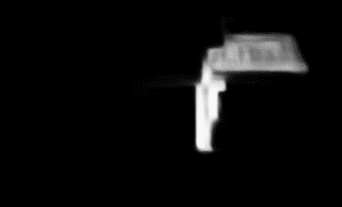
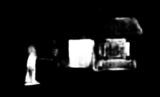
.083	.501	.541
BBSNet [10]	PGAR [4]	UCNet [61]

Figure 1: An example of a challenging input from RGB-D dataset with multiple candidate salient objects and noisy depth. As shown in the third row, undesirable depth has adversely affected the saliency prediction, where our  PASNet visual results in the second row are much closer to the GT with higher F-measure rates. PASNet (M1) and PASNet (M2) refer to RGB-D with original and synthetic depth.

Visual saliency refers to the most noticeable and discernible contents of image data distinguishable from the background. It is often termed Salient Object Detection (SOD), as the noticeable contents are different kinds of objects inside an image. Salient objects include humans, animals, and other general object categories within an image as foreground. SOD methods [36, 58, 42, 76, 10, 51, 31] aim to extract useful features from a given RGB or a pair of RGB and depth images to predict a binarized or gray-scale saliency map of the corresponding input.

To achieve effective SOD, RGB or RGB-D images are processed using various soft computing techniques, where deep models [45, 5] have achieved the best results. Whereas, RGB-D-based SOD has recently attracted the attention of many experts due to the importance of depth data in predicting accurate saliency maps when processed composedly with RGB data, providing complementary information for objects’ appearance, thereby enhancing the SOD method’s performance. Moreover, the mainstream RGB-D approaches introduce multi-stream architectures to extract RGB and depth features and apply various fusion mechanisms to assist RGB data with depth clues. Previous research techniques input RGB and depth data, apply fusion at early [61, 60], intermediate (multiple stages) [63, 66], or later stages [48] of the neural network architecture to achieve optimal detection. Recently, Zhang et al. [61] integrated RGB and depth channels at the start of the network and processed six-channel input, while in their supplementary network, the authors extract distributions of RGB images as well as depth clues.

With RGB-D-based techniques, certain limitations are associated, such as additional computation is required to process depth data and, fore-mostly, the depth sensor data acquisition for generating saliency maps. Conversely, CNN-based RGB saliency models can quickly fail in challenging scenarios due to a lack of appearance cues and dependency over visual cues only. Similarly, RGB-based saliency detection methods get misled in cluttered backgrounds due to the complex salient object’s appearance.

To the best of our knowledge, no single end-to-end method in SOD literature exists that takes RGB input only and generates its corresponding depth, followed by final saliency prediction using both channels. Following [56], Zhang et al. [66] introduced RGB-D SOD without Depth, a simple network that learns to predict multiple outputs during testing; but depend on the depth data for the network during training.

This article overcomes the limitations mentioned earlier by introducing novel transformer-CNN features with a pyramidal attention network for effective SOD. The proposed model, Pyramidal Attention Saliency, abbreviated as, PASNet is specifically designed to remove the dependency over depth data, thereby increasing our model’s application domains and practicability. In simple scenarios, our network’s RGB flavor can be used to create accurate saliency maps. While in highly challenging scenarios, where RGB information is not sufficient for fine saliency detection, our network’s RGB-D flavor generates depth from RGB and complementary features from the same depth network to support the RGB features at various levels before optimal saliency region extraction. Furthermore, it is a well-known fact that the encoder structure of the SOD model has a considerable influence while producing saliency maps as information lost during the encoding process cannot be recovered in the decoder. Therefore, along with the focus on decoder [55], the encoder part should be carefully designed, as, in PASNet, we present a transformer encoder to extract multi-level features with pyramidal attention structure for image feature enhancement.

Our contributions are highlighted as follows:

• We are the first to introduce the RGB-D SOD model without actually acquiring depth data as input, thus, predicting fine saliency using only single RGB input.

• Our encoder network considers both high and low-level CNN and transformer backbone features to process them using pyramidal transformer attention.

• We achieve SOTA results on both RGB and RGB-D SOD benchmarks, validating the proposed model effectiveness and practical applicability.

2 Related Work

The SOD techniques can be roughly categorized from the perspective of input data into i) RGB-D methods, ii) Hybrid methods, and iii) RGB methods. We provide the SOD models similar to our approach and justify the uniqueness of our model from the current state-of-the-art.

RGB-D Methods: The RGB-D methods need RGB and depth data for generating saliency maps, where both modalities are dependent on each other. The depth modality is specifically considered to extract the 3D layout and structural information from the input images and aid the RGB channels in generating final saliency. Currently, mainstream RGB-D SOD methods apply Convolutional Neural Networks (CNN) [40] due to their enhanced image representation abilities, compared to handcrafted features [38, 11, 6] which provides limited performance for complex scenarios. Some RGB-D methods merge depth and RGB channels in early stages, considering RGB-D pair as a multi-channeled input [33, 43]. Others apply late [16] or multi-stream fusion approaches [10] to effectively utilize the complimentary depth information [39, 3, 40]. These mentioned methods require depth maps as input while generating saliency maps during training and testing. The RGB-D methods’ accurate predictions are highly dependent on the depth data cues, and any noise in the depth data results in mispredictions. In some cases, particularly noisy regions are considered salient objects by the model. Thus, for an RGB-D SOD model, the dependency of depth data affects the performance in many scenarios, despite the higher computational complexity and expensive resources required for depth sensor data acquisition.

Hybrid Methods: If trained on RGB-D data, the model is considered a hybrid and can predict saliency maps without acquiring depth data. These approaches tend to eliminate the dependency of supplementary depth cues while generating output. Initially, Ziao et al. [56] introduced the concept of leveraging depth information with RGB data to enhance a model’s performance for SOD task, based on traditional saliency features and without any end-to-end methodology for depth and saliency prediction. Similarly, A2dele [41], an adaptive and attentive depth distiller, is introduced in recent research, aiming at the RGB-D network’s efficiency and reducing the dependency over depth data during testing. Their main objective is to provide an effective network that only processes RGB stream rather than involving depth stream during the testing procedure.

Very recently, Zhang et al. [66] presented a deep RGB-D network that learns to predict saliency maps as well as depth images from an RGB-D input; thus, the network takes RGB-D data while training and does not require depth data during evaluation, but results without depth input are significantly lagging behind the RGB-D SOTA. Furthermore, deep RGB-D w$/$o depth methods still have the primary deficiency of depth sensory data dependency during training. It is not easy to install multiple sensors or a single sensor with multiple functionalities in some real-world environments due to marginally higher costs. Finally, a very recent research [66] fuses the actual predicted depth at the last stages, making their model biased towards the RGB channel information.

RGB Methods: Traditionally, salient object detection relied on the RGB input only for decades. So far, a handful CNN based research works employed RGB data only as input to produce refined saliency maps. The CNN models follow the traditional encoder-decoder architecture while generating saliency, where the network is used as an encoder to extract initial, middle, and high-level features, followed by upsampling strategies to generate saliency maps [19, 69]. Different from traditional decoders, Wu et al. [55] introduced a partial decoder that only considers features extracted from deeper CNN layers, generating initial and final saliency maps. The initial saliency is processed applying a holistic attention module which is then fused through element-wise multiplication with encoder features and their proposed partial decoder for the final saliency map. Many researchers focus on the edge information [69], while others apply boundaries-directed features learning Siamese networks and modified fusion strategies to generate binarized saliency maps [25].

The existing SOD literature advocates that current deep models are heavily dependent on depth clues (see Figure 1 3^rd row) while generating refined saliency maps, mainly processing RGB and depth input via multi-stream networks. Herein, we show that providing depth data should only enhance the prediction performance (Figure 1, 2^nd row), and refined saliency maps can be acquired using RGB input. Furthermore, RGB-D models need both RGB and depth simultaneously to predict saliency. In contrast, we propose to estimate depth from the RGB image and extract features from synthetic depth to enhance the encoder’s performance. Although there are previous attempts [66, 56, 41] to remove the depth input reliance and ease their practical applicability, these are hybrid (RGB+RGB-D) models i.e., they process depth during training and have comparatively higher error rates and minimal performance for challenging RGB datasets.

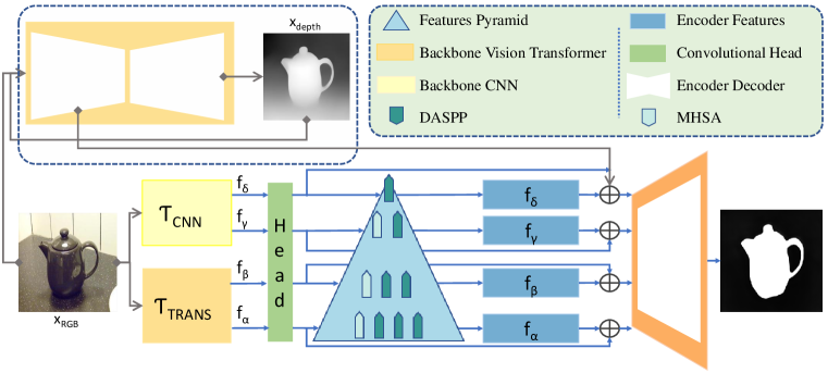
Figure 2: The proposed SOD framework. The encoder module takes an RGB image and passes it to a depth predictor ($\Delta$) to acquire $X_{depth}$, a CNN model ($\tau_{CNN}$) with a ResNet backbone produces $f_{\alpha}$ and $f_{\beta}$ feature vectors, and the transformer encoder ($\tau_{Trans}$) generates $f_{\gamma}$ and $f_{\sigma}$ features. We transform these features to equal channels using a head with sequential convolutional operations. These outputs are then transformed to highly salient features, effective for SOD using the proposed pyramidal block of DASPP and MHSA $\rho$. We employ skip connections after acquiring features from $\rho$ and finally concatenate the depth features extracted from an intermediate stage of $\Delta$ model using a synthetic depth image with the $f_{\sigma}$ features. The decoder module continuously fuses information, employ and upsample them gradually with residual channel attention at multiple stages before final saliency prediction. We applied a weighted fusion strategy over different losses to update our model’s parameters.

3 Methodology

In this section, we describe the proposed SOD model. We employ a pyramidal architecture to incorporate CNN and transformer backbone features. First, we comprehensively introduce our framework explain each component of our model in detail, followed by the proposed pyramid structure for feature refining and saliency extraction.

3.1 Overview

The proposed network consists of several components: i) feature extraction from the backbone network with customized dense connections; ii) pyramid block for encoder feature refining; and iii) upsampling and feature fusion in the decoder. In the case of the depth requirement, our network generates a corresponding depth map using a pre-trained ViT-based monocular depth estimation model [44] and extracts intermediate features from the same model to be fused with the RGB module before decoding. The overall process is visualized in Figure 2 and explained in subsequent sections.

3.2 Pyramidal Self-Attention

Transformer networks process bag-of-words$/$tokens representations of input data [46], where image features play tokens in case of ViT. Herein, following the findings of [44], we extract deep pixel features from the input RGB image $I_{RGB_{h\times w}}$ using a pre-trained embedding network [17] and use them as tokens $t=\{t_{0},...,t_{N_{p}}\}$, where $N_{p}=\frac{\textit{h}\times\textit{w}}{p^{2}}$, with height $h$, width $w$ and $p$ refers to the patch size considered in our network. The encoder network produces $f_{\alpha},f_{\beta},f_{\gamma},f_{\sigma}=\tau(t)$, where $\tau$ refers to the proposed encoder. The $f_{\alpha},f_{\beta}$ are CNN features acquired from the feature embedding network’s $b_{i}$ and $b_{j}$ blocks and $f_{\gamma},f_{\sigma}$ are transformer stages $s_{i}$ and $s_{j}$. To decode $f_{\gamma}$ and $f_{\sigma}$ features from the transformer layers, we use a patch un-embedding strategy.

To enable maximum information flow between CNN features and transformer blocks, we embed dense connections as follows:

$$\begin{split}f_{\alpha}&=\tau_{CNN_{bi}}(I_{RGB}),\\ f_{\beta}&=\tau_{CNN_{bj}}(f_{\alpha}).\end{split}$$ (1)

So far, we have two kinds of feature vectors comprising initial edge information $(f_{\alpha},f_{\beta})$, we extract shapes and structure of objects, and global receptive fields $(f_{\gamma},f_{\sigma})$ as

$$\begin{split}f_{\gamma}&=\tau_{Trans_{si}}(f_{\alpha}\oplus f_{\beta})),\\ f_{\sigma}&=\tau_{Trans_{sj}}(f_{\alpha}\oplus f_{\beta}\oplus f_{\gamma})),\end{split}$$ (2)

where $\oplus$ is the concatenation operation. These four extracted features have a common trans-head to refine and balance the channels for the proposed pyramidal attention blocks. The trans-head has three convolutional layers, each followed by batch normalization and ReLU activation.

Based on the assumption that initial low-level features $(f_{\alpha},f_{\beta})$ demand further refining and the later stage transformer features$(f_{\gamma},f_{\sigma})$ only need booster layers to enhance the existing representations. We employ pyramid attention block $P_{\rho}$ to finally acquire the encoder features. The $P_{\rho}$ contains multi-scale Dense Atrous Spatial Pyramid Pooling (DASPP) layers and multi-headed self-attention (MHSA) at the end of each $P_{\rho}$ block except the final $f_{\sigma}$ features. Since the convolutional features need additional attention, they fit into the pyramid’s base with multiple DASPP modules followed by an attention mechanism. The last stages of transformer features are utilized using a single DASPP and MHSA module. As $f_{\sigma}$ features are already enhanced enough; therefore, only a single DASPP module is employed for further feature enhancement. The overall structure of $P_{\rho}$ is shown in Eq. 3.

Once the refined features are extracted from the RGB input, we enrich $f_{\sigma}$ features via depth estimation ($\Delta$) model’s features. It is noteworthy that depth is not accompanied (i.e., actual depth acquired via a depth sensor) with the input image in the RGB-D dataset; instead, it is synthetically generated from the $\Delta$ model. Due to simplicity, we do not create a separate network to process depth data individually, which can be a significant future direction for RGB-D SOD models. The concatenation at this point aids the $f_{\sigma}$ with fine-grained depth information, producing more refined representations (see Figure 1 second row).

Our main objective in the proposed encoder network is not to lose any information, as it cannot be recovered during the decoding procedure. Therefore, we consider information about edges filtered by the initial CNN blocks and employ several transformer layers to extract receptive fields to keep track of the varied size of objects. Thus, combining convolutional and transformer layers’ features enables utilizing larger receptive fields when compared to regular convolutions and also design dependencies between spatially distinct features. Finally, the proposed pyramid structured attention boosts the features for the SOD problem by applying DASPP [59] for receptive fields capturing from the overall image and multi-head attention for acquiring salient information from paired feature representations.

3.3 Fusion Attention

Hence, the encoder network is very dense, extracting various features. Therefore, we only focus on fusing the encoder features in the decoder network before generating the final saliency. The decoder receives $f_{\alpha},f_{\beta},f_{\gamma}$, and $f_{\sigma}$ features, progressively concatenating from the fusion of shallower to deeper layers. After each concatenation branch, our network employs the residual channel attention module to capture spatial and channel dependencies between pixel locations and different channels of the input feature maps. We achieve the final saliency map $S$ by gradually upsampling the features during concatenation, as given below mathematically.

$$\begin{split}S_{i}&=\theta(f_{\sigma}\oplus f_{\gamma}),\\ S_{i+1}&=\theta(\cup(S_{i}\oplus f_{\beta}),\\ S_{i+2}&=\theta(S_{i+1}\oplus f_{\alpha}),\\ S&=\cup_{h\times w}(C(S_{i+2})),\end{split}$$ (4)

where $\cup$ is the upsampling operation, $\theta$ refers to the residual channel attention module, and $C$ is the balancing convolution to generate a single channel saliency map $S$.

DUT-RGBD
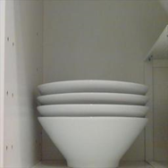
NJUD2K
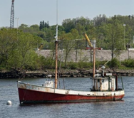
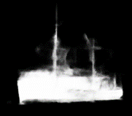
NLPR
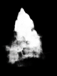
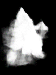
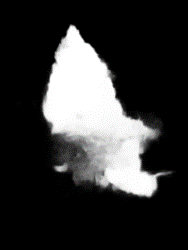
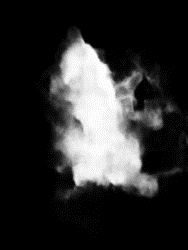
SIP
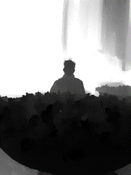
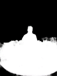
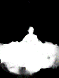
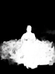
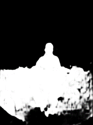
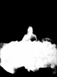
	Image	Depth	GT	DCF [20]	BBSNet [10]	PGAR [4]	UCNet [61]	D3Net [9]	PASNet

Figure 3: Visual comparison of our PASNet with SOTA models using the most challenging images from RGB-D datasets. Our results are more close to the groundtruth. Our saliency maps have fine details and clear edges as compared to the state-of-the-art algorithms.

3.4 Objective Function

The proposed objective function is the weighted fusion of several loss functions defined below for input $y$ and ground truth $x$ images.

$$\ell_{{total}_{(y,x)}}=\epsilon_{1}\ell_{st}+\epsilon_{2}\ell_{ssim}+\epsilon_{3}\ell_{2}+\epsilon_{4}\ell_{se},$$ (5)

where $\epsilon$ is the constant having values of $\epsilon_{1}=0.2$, $\epsilon_{2}=0.3$, $\epsilon_{3}=0.2$, and $\epsilon_{4}=0.3$.

The structure loss $\ell_{st}$ focuses on global structure optimization instead of aiming at a single pixel, thereby being significantly immune towards unbalanced distributions. We adopt structure loss from [53], where weights are assigned to hard pixels to highlight their importance, instead of treating all pixels equally and ignoring the difference between pixels. The $\ell_{st}$ loss is given as

$$\ell_{{st}_{(y,x)}}=1-\frac{\sum_{i=1}^{H}\sum_{j=1}^{W}(x_{ij}y_{ij})(1+\Psi\omega_{ij})}{\sum_{i=1}^{H}\sum_{j=1}^{W}(x_{ij}+y_{ij}-x_{ij}y_{ij})(1+\Psi\omega_{ij})},$$ (6)

where $\Psi$ is a hyperparameter and $\omega$ are the weights.

Furthermore, different from pixel-wise comparison losses such as the Euclidean distance, we employ Structural Similarity Index Measure (SSIM) as a loss function to compute the negation of similarity between $y$ and $x$ and update the model based on their difference.

$$\ell_{{ssim}_{(y,x)}}=1-\frac{(2\mu_{y}\mu_{x}+c_{1})(2\varsigma_{y}{yx}+c_{2})}{(\mu_{y}^{2}+\mu_{x}^{2}+c_{1})(\varsigma_{y}^{2}+\varsigma_{y}{x}^{2}+c_{2})}.$$ (7)

In Eq. 7, $\mu_{i}$ and $\mu_{t}$ represent the average, $\varsigma_{it}$ is the covariance, $\varsigma_{i}^{2}$ and $\varsigma_{t}^{2}$ represent variance of input $y$ and the ground truth image $x$, respectively. Herein, $c_{1}=(k_{1},L)^{2}$, $c_{2}=(k_{2},L)^{2}$ that are two variables to neutralize the division in case of weak denominator. Finally, $L$ is a dynamic range of pixel values and $k_{1}=0.01,k_{2}=0.03$.

Moreover, $\ell_{2}$ refers to $\ell_{ssim}$ regularization. Due to the involvement of multiple features, our network becomes complex and prone to overfitting; therefore, we adopt $\ell_{2}$ regularization in our loss function to avoid such problems. Finally, edge-aware smoothness loss is adopted from [15, 52], referred to as $\ell_{se}$ in Eq. 5, which makes the distinctions between objects smoother using disparity gradients. Herein, $\epsilon$ is used to assign weights multiplied with each loss value when calculating the final objective function for the model update.

3.5 Implementation Details

Inspired by the CNN-based SOD models’ [60, 9, 45] backbone strategies, we employ pre-trained DPT [44], that is trained on a large-scale semantic segmentation dataset as the ViT networks perform well when trained using large-scale datasets [8]. For feature extraction, following [44], we extract transformer tokens from a ResNet50 pre-trained model [17]. We utilize the same model’s initial two blocks $b_{i},b_{j}=1,2$ to extract $f_{\alpha},f_{\beta}$ features. In case $\tau_{TRANS}$, $f_{\gamma},f_{\sigma}$ are transformer stages $s_{i},s_{j}=9,12$ features. It should be noted that we embed depth transformer features from stage $s=12$ of depth estimator backbone model $\Delta$ into $f_{\sigma}$ features to enhance the representations of existing features. The resolution of output features is $h\times\frac{1}{2^{n}}$, where $n=1,2,3,$ and $4$ for $f_{\alpha},f_{\beta},f_{\gamma},$ and $f_{\sigma}$, respectively with $D_{feat}=256$ features’ dimensions.

Table 1: Quantitative results of our algorithm against competing methods. The symbols E_α, F_β, and S_γ refer to the E-measure, F-measure, and S-measure. The (Red color represents the best results and the Blue color is for the second-best results in each block i.e. RGB-D, RGB, and Hybrid models.

	Methods	DUT-RGBD [40]				NJUD2K [21]				NLPR [38]				SIP [9]
		E${}_{\alpha}\uparrow$	F${}_{\beta}\uparrow$	S${}_{\gamma}\uparrow$	MAE$\downarrow$	E${}_{\alpha}\uparrow$	F${}_{\beta}\uparrow$	S${}_{\gamma}\uparrow$	MAE$\downarrow$	E${}_{\alpha}\uparrow$	F${}_{\beta}\uparrow$	S${}_{\gamma}\uparrow$	MAE$\downarrow$	E${}_{\alpha}\uparrow$	F${}_{\beta}\uparrow$	S${}_{\gamma}\uparrow$	MAE$\downarrow$
RGB-D	DF [43]	.	.465	.	.185	.700	.653	.763	.140	.757	.664	.806	.079	.565	.465	.653	.185
	CTMF [16]	.	.608	.	.139	.846	.779	.849	.085	.840	.740	.860	.056	.704	.608	.716	.139
	PCF [1]	.	.814	.	.071	.895	.840	.877	.059	.887	.802	.874	.044	.878	.814	.842	.071
	MMCI [3]	.	.771	.	.086	.851	.793	.858	.079	.841	.737	.856	.059	.845	.771	.833	.086
	CPFP [68]	.	.821	.	.064	.910	.850	.878	.053	.918	.840	.888	.053	.893	.821	.850	.064
	CPD [55]	.	.872	.	.042	.	.874	.	.051	.	.878	.	.028	.	.884	.	.043
	TANet [2]	.	.803	.	.075	.895	.841	.879	.059	.902	.802	.886	.044	.870	.803	.835	.075
	AFNet [48]	.	.702	.	.118	.867	.827	.822	.077	.851	.755	.799	.058	.793	.702	.720	.118
	DMRA [40]	. 888	.883	.927	.048	.920	.873	.886	.051	.940	.865	.899	.031	.844	.811	.806	.085
	ATSA [63]	.	.918	.916	.032	.	893	.885	.040	.	.876	.909	.028	.	.871	.849	.053
	PGAR [4]	.933	.914	.899	.035	.940	.893	.909	.042	.	.885	.917	.024	.	.854	.838	.055
	UCNet [61]	.	.	.871	.	.936	.886	.897	.043	.951	.831	.920	.025	.914	.867	.875	.051
	S2MA [30]	.935	.899	.904	.043	.930	.889	.894	.054	.953	.902	.916	.030	.919	.877	.872	.058
	JL-DCF [13]	.941	.910	.906	.042	.944	.904	.902	.041	.963	.918	.925	.022	.919	.877	.880	.058
	SSF-RGBD [64]	.950	.923	.915	.033	.935	.896	.899	.043	.953	.896	.915	.027	.870	.786	.799	.091
	BBSNet [10]	.912	.870	.923	.058	.949	.919	.921	.035	.961	.918	.931	.023	.922	.884	.879	.055
	Cas-Gnn [34]	.953	.926	.920	.030	.948	.911	.911	.039	.955	.906	.923	.025	.919	.879	.875	.051
	CMW [23]	.864	.779	.797	.098	.927	.871	.870	.061	.951	.903	.917	.029	.804	.677	.705	.141
	DANet [72]	.939	.904	.899	.042	.935	.898	.899	.046	.955	.904	.920	.028	.918	.876	.875	.055
	cmMS [22]	.940	.913	.912	.036	.897	.936	.900	.044	.955	.904	.919	.028	.911	.876	.872	.058
	UCNet-2 [60]	.	.864	.	.034	.937	.893	.902	.039	.952	.893	.917	.025	.927	.877	.883	.045
	SP-Net [74]	.	.	.	.	.954	.935	.925	.028	.959	.925	.927	.021	.930	.916	.894	.043
	DA-MMFF [45]	.950	.926	.921	.030	.923	.901	.903	.039	.950	.897	.918	.024	.	.	.	.
	DCF [20]	.952	.926	.	.030	.922	.897	.	.038	.956	.893	.	.023	.920	.877	.	.051
	HFNet [75]	.934	.885	.900	.044	.902	.859	.898	.053	.934	.839	.897	.038	.904	.850	.857	.071
	VST [31]	.969	.948	.943	.024	.951	.920	.922	.035	.962	.920	.943	.024	.944	.915	.904	.040
	PASNetM1	.966	.944	.917	.028	.938	.892	.867	.051	.966	.921	.913	.021	.987	.956	.936	.016
RGB	DSS [18]	.	.732	.803	.127	.	.776	.769	.108	.	.755	.838	.076	.	.	.	.
	Amulet [65] .	.	.803	.813	.083	.	.798	.827	.085	.	.722	.838	.062	.	.	.	.
	R3Net [7] .	.	.781	.819	.113	.	.775	.770	.092	.	.649	.846	.101	.	.	.	.
	PiCANet [29] .	.	.826	.878	.080	.	.806	.872	.071	.	.761	.871	.053	.	.	.	.
	PAGRN [70] .	.	.836	.	.079	.	.827	.	.081	.	.795	.	.051	.	.	.	.
	PoolNet [27] .	.	.871	.	.049	.	.850	.	.057	.	.791	.	.046	.	.	.	.
	AFNet [12] .	.	.851	.	.064	.	.857	.	.056	.	.807	.	.043	.	.	.	.
	CPD [55] .	.911	.865	.875	.055	.905	.905	.863	.060	.925	.866	.893	.034	.	.	.	.
	EGNet [69] .	.	.866	.872	.059	.	.846	.840	.060	.	.800	.880	.047	.	.876	.	.049
	MSI-Net [37] .	.900	.861	.875	.058	.906	.859	.870	.057	.914	.854	.886	.041	.	.	.	.
	DCF [20] .	.	.	.	.	.	.869	.	.046	.	.855	.	.028	.	.839	.	.063
	PASNet	.966	.940	.903	.033	.946	.907	.891	.040	.964	.921	.912	.024	.987	.955	.930	.018
Hybrid	A2dele [41]	.	.892	.885	.042	.	.884	.871	.051	.	.878	.899	.028	.	.884	.829	.043
	DASNet [67]	.	.	.	.	.	.894	.902	.042	.	.907	.929	.021	.	.	.	.
	DeepRGB-D [66]	.902	.853	.864	.072	.927	.876	.886	.050	.936	.882	.906	.038	.	.	.	.
	PASNetM2	.966	.942	.903	.029	.948	.908	.891	.040	.962	.917	.912	.021	.988	.958	.930	.015

Table 2: Performance comparison on RGB datasets against RGB methods for MAE metric. The lower ($\downarrow$) is the value for MAE, the better the accuracy). Red, Blue, and Magenta colors show first, second, and third best performance.

Methods	ECSSD [57]	HKU-IS[24]	DUTS-TE [47]	PASCAL-S [26]
NLDF [35]	.051	.041	.055	.083
DSS [18]	.051	.043	.050	.081
BMPM [62]	.044	.039	.049	.074
Amulet [65]	.057	.047	.062	.095
SRM [49]	.054	.047	.059	.085
PiCANet [29]	.035	.031	.040	.072
DGRL [50]	.043	.037	.051	.074
CPD [55]	.037	.034	.043	.074
EGNet [69]	.037	.031	.039	.080
TSPOANet [32]	.047	.039	.049	.082
AFNet [12]	.042	.036	.045	.076
PoolNet [27]	.042	.032	.041	.076
BASNet [42]	.037	.032	.047	.083
GateNet [71]	.038	.031	.037	.071
CSNet [14]	.033	.	.037	.073
LDF [54]	.034	.028	.034	.067
MSI-Net [37]	.034	.029	.037	.071
ITSD [73]	.035	.031	.041	.071
VST [31]	.037	.030	.037	.067
SDC [25]	.034	.030	.037	.111
PoolNet-R+ [28]	.040	.034	.039	.068
PASNetRGB	.030	.029	.039	.068

4 Experiments

4.1 Setup

Training details: We implement our method in the PyTorch deep learning framework with an NVIDIA GeForce RTX 3090 GPU. Our initial training settings are inspired from [61]. We use an ADAM optimizer with 0.9 momentum, the initial learning rate is set to 5$e^{-5}$, and the model is trained for 25 epochs. The training images are resized to a standard 224 $\times$ 224. The ResNet50 [17] is used as the backbone with the pre-trained ImageNet weights in the CNN module, while in the Transformer module, we use [44]. After each epoch, the learning rate is adjusted with a 10% decrease, and the batch size is six.

Datasets: We carry out experiments on four benchmark RGB-D datasets including three standard such as DUT-RGBD [40], NJUD2K [21], NLPR [38], and newly introduced SIP [9]. We also compare on four datasets, that are widely used for RGB SOD method evaluation, including ECSSD [57], HKU-IS [24], DUTS-TE [47], and PASCAL-S [26]. We follow the provided training and testing dataset split for each one [9].

Evaluation Metrics: We evaluate our methods on three widely used metrics: Mean Absolute Error (MAE), standard F-measure (F_β), and E-measure (E_α). We have verified the results of our methods via MATLAB and Python evaluation toolboxes. It should be noted that the lower the (MAE) the better it is and vice versa for (F_β) (S_α), and (E_α).

4.2 Comparisons

We compare our results with 41 methods on RGB-D datasets and 21 algorithms employing RGB datasets, comprising recent deep learning-based models.

Image	Depth	GT	SD	M2	M1

Figure 4: Visual scenarios with $M2$’s more accurate predictions when compared to $M1$. The clearly observable difference is due to the noise in input depth data. SD refers to synthetic depth.

4.2.1 Quantitative Comparisons

RGB-D Saliency: For RGB-D SOD, we compare our method with 41 deep learning models, and since traditional hand-crafted feature-based methods are not effective and accurate enough, we exclude them for simplicity. To ensure a fair comparison, we mostly report the results of these methods from their papers or follow existing articles [20, 60, 31]. Furthermore, it is worth noting that there are ten RGB methods performing experiments on RGB-D datasets, while the closest works to our approach are considered hybrid models.

The performance comparisons on the RGB-D datasets are given in Table 1, where we reported three sections due to the difference in the SOD input. When compared to RGB and hybrid methods utilizing RGB-D datasets, we achieved the best results on all reported metrics, surpassing SOTA methods by a large margin on some metrics. Similarly, we receive better performance when we generate saliency using RGB-D with original depth i.e. second best results on DUT-RGBD [40]. On the NJUD [21] dataset, we lag behind some current methods, but it is noteworthy that we did not use any multi-stream architecture to process depth data, as our primary objective is to eradicate dependency over depth data. On the NLPR [38] dataset, we achieved SOTA on MAE and $E_{\alpha}$ and held second best in terms of F-measure, as [74] achieved 0.004 higher $F_{\beta}$ from our model. Finally, we set a new SOTA over SIP [9] dataset.

RGB Saliency: Our proposed model is compared with 21 RGB-based SOD methods in Table 2 on RGB datasets, which shows significantly reduced error rates and top performance on three ECSSD [57], HKU-IS [24], and PASCAL-S [26] datasets except DUTS-TE [47]. Where PASNet is ranked as the third-best against competing methods. Thus, it can be concluded that the proposed model is also applicable in challenging scenarios that can be effectively functional and independent of the depth module.

4.2.2 Qualitative Comparisons

We present visual outcomes of our model against SOTA for four challenging images with noisy depth and complex background, similar or multiple salient objects, and distant objects. Figure 3 shows how accurately PASNet predicts saliency maps. PASNet  predicts high-quality, smooth saliency of the input image with similar background and foreground (1^st and 3^rd rows), where top-ranked RGB-D models produced very coarse predictions. Likewise, PASNet  correctly identified distant objects (2^nd row) well, even though the accompanying depth of corresponding RGB has much noise, confusing the depth-dependent deep models to produce non-smooth dispersed predictions. Similarly, for an object hiding behind informative background (4^th row), our method produced exactly similar saliency as ground truth, whereas the compared SOTA produced limited results. It should be noted that our method produces similar or very close saliency maps to the ground truth. Therefore, analyzing qualitative and quantitative results demonstrates the proposed model’s effectiveness and robustness.

4.2.3 Ablation Study

We carried out several ablation studies to analyze the effect of the various parameters for the proposed framework. $M1$ and $M2$ refer to experimentation in terms of data input i.e., including depth data features to predict the final saliency, provided in Table 1. $M3$ refers to the effect of the proposed pyramidal attention block, where visual qualitative results are presented in Figure 4, and detailed quantitative ablation results of various models are given in Figure 5. Next, we provide our analysis.

Original vs. Synthetic Depth: Basically, the proposed model processes only RGB input, where in some cases, we integrated depth data to see the effect on output predictions. Depth data for sure increases the smoothness of saliency prediction, and hence it improves the performance (see Figure 4). Firstly for $M1$, we used the original depth data provided in RGB-D datasets and achieved excellent performance compared to SOTA and other variants of our model, but it comes at the cost of depth data dependency. Next, for $M2$, we generated depth from the input RGB image and achieved a comparable decrease in performance against $M1$, but still, this model outperformed SOTA models of its kind. In the case of NJUD2K and SIP datasets, $M2$ has better performance due to noise in the original depth, as shown in Figure 4. Although our RGB-D methods have a lower dependency on depth features, the saliency prediction performance is still adversely affected by noise or improper depth information.

Effect of Proposed Pyramidal Attention ($P_{\rho}$): To analyze the impact of the proposed pyramidal attention block features performance, we exclude $P_{\rho}$ from PASNet named as $M3$. It is observable from Figure 5 that the error rates significantly increase due to the non-effective feature representations directly acquired from ViT and CNN networks without post-enhancement using $P_{\rho}$. The pyramidal attention block reduces the error rates by an average of 4.525% on four RGB-D datasets.

Figure 5: Error rates of ablation studies conducted using RGB-D datasets.

5 Conclusion

In this paper, we rethink RGB and RGB-D SOD from a new perspective, employing multi-level CNN and pyramidal attention features in the encoder. Our method is applicable to RGB and RGB-D SOD, where we acquire a single RGB input, estimate its depth, and fuse depth features with the RGB model to enhance saliency prediction results. Moreover, our proposed decoder architecture fuses encoder features at multi-levels and gradually upsample to predict saliency maps with refined edges and focus on the essential parts of the input image. To the best of our knowledge, we are the first to eliminate the acquisition of multiple inputs for RGB-D SOD and achieved state-of-the-art results over both RGB and RGB-D SOD datasets.

Acknowledgements

This work was supported by Institute of Information & communications Technology Planning & Evaluation (IITP) grant funded by the Korea government(MSIT) $[$No. 2020-0-00062, Project Name$:$ Development of data augmentation technology by using heterogeneous data and external data integration$]$.

References

- [1] Hao Chen and Youfu Li. Progressively complementarity-aware fusion network for rgb-d salient object detection. In CVPR, pages 3051–3060, 2018.
- [2] Hao Chen and Youfu Li. Three-stream attention-aware network for rgb-d salient object detection. TIP, pages 2825–2835, 2019.
- [3] Hao Chen, Youfu Li, and Dan Su. Multi-modal fusion network with multi-scale multi-path and cross-modal interactions for rgb-d salient object detection. PR, pages 376–385, 2019.
- [4] Shuhan Chen and Yun Fu. Progressively guided alternate refinement network for rgb-d salient object detection. In ECCV, pages 520–538. Springer, 2020.
- [5] Yupeng Cheng, Huazhu Fu, Xingxing Wei, Jiangjian Xiao, and Xiaochun Cao. Depth enhanced saliency detection method. In Proceedings of international conference on internet multimedia computing and service, pages 23–27, 2014.
- [6] Arridhana Ciptadi, Tucker Hermans, and James M Rehg. An in depth view of saliency. Georgia Institute of Technology, 2013.
- [7] Zijun Deng, Xiaowei Hu, Lei Zhu, Xuemiao Xu, Jing Qin, Guoqiang Han, and Pheng-Ann Heng. R3net: Recurrent residual refinement network for saliency detection. In IJCAI, pages 684–690, 2018.
- [8] Alexey Dosovitskiy, Lucas Beyer, Alexander Kolesnikov, Dirk Weissenborn, Xiaohua Zhai, Thomas Unterthiner, Mostafa Dehghani, Matthias Minderer, Georg Heigold, Sylvain Gelly, et al. An image is worth 16x16 words: Transformers for image recognition at scale. arXiv preprint arXiv:2010.11929, 2020.
- [9] Deng-Ping Fan, Zheng Lin, Zhao Zhang, Menglong Zhu, and Ming-Ming Cheng. Rethinking rgb-d salient object detection: Models, data sets, and large-scale benchmarks. TNNLS, 2020.
- [10] Deng-Ping Fan, Yingjie Zhai, Ali Borji, Jufeng Yang, and Ling Shao. Bbs-net: Rgb-d salient object detection with a bifurcated backbone strategy network. In European Conference on Computer Vision, pages 275–292. Springer, 2020.
- [11] David Feng, Nick Barnes, Shaodi You, and Chris McCarthy. Local background enclosure for rgb-d salient object detection. In Proceedings of the IEEE conference on computer vision and pattern recognition, pages 2343–2350, 2016.
- [12] Mengyang Feng, Huchuan Lu, and Errui Ding. Attentive feedback network for boundary-aware salient object detection. In CVPR, pages 1623–1632, 2019.
- [13] Keren Fu, Deng-Ping Fan, Ge-Peng Ji, and Qijun Zhao. Jl-dcf: Joint learning and densely-cooperative fusion framework for rgb-d salient object detection. In CVPR, pages 3052–3062, 2020.
- [14] Shang-Hua Gao, Yong-Qiang Tan, Ming-Ming Cheng, Chengze Lu, Yunpeng Chen, and Shuicheng Yan. Highly efficient salient object detection with 100k parameters. In ECCV, pages 702–721. Springer, 2020.
- [15] Clément Godard, Oisin Mac Aodha, and Gabriel J Brostow. Unsupervised monocular depth estimation with left-right consistency. In CVPR, pages 270–279, 2017.
- [16] Junwei Han, Hao Chen, Nian Liu, Chenggang Yan, and Xuelong Li. Cnns-based rgb-d saliency detection via cross-view transfer and multiview fusion. TCYB, pages 3171–3183, 2017.
- [17] Kaiming He, Xiangyu Zhang, Shaoqing Ren, and Jian Sun. Deep residual learning for image recognition. In CVPR, pages 770–778, 2016.
- [18] Qibin Hou, Ming-Ming Cheng, Xiaowei Hu, Ali Borji, Zhuowen Tu, and Philip HS Torr. Deeply supervised salient object detection with short connections. In CVPR, pages 3203–3212, 2017.
- [19] Tanveer Hussain, Saeed Anwar, Amin Ullah, Khan Muhammad, and Sung Wook Baik. Densely deformable efficient salient object detection network. arXiv preprint arXiv:2102.06407, 2021.
- [20] Wei Ji, Jingjing Li, Shuang Yu, Miao Zhang, Yongri Piao, Shunyu Yao, Qi Bi, Kai Ma, Yefeng Zheng, Huchuan Lu, et al. Calibrated rgb-d salient object detection. In CVPR, pages 9471–9481, 2021.
- [21] Ran Ju, Ling Ge, Wenjing Geng, Tongwei Ren, and Gangshan Wu. Depth saliency based on anisotropic center-surround difference. In ICIP, pages 1115–1119, 2014.
- [22] Chongyi Li, Runmin Cong, Yongri Piao, Qianqian Xu, and Chen Change Loy. Rgb-d salient object detection with cross-modality modulation and selection. In ECCV, pages 225–241. Springer, 2020.
- [23] Gongyang Li, Zhi Liu, Linwei Ye, Yang Wang, and Haibin Ling. Cross-modal weighting network for rgb-d salient object detection. In European Conference on Computer Vision, pages 665–681. Springer, 2020.
- [24] Guanbin Li and Yizhou Yu. Visual saliency based on multiscale deep features. In CVPR, pages 5455–5463, 2015.
- [25] Junxia Li, Ziyang Wang, Zefeng Pan, Qingshan Liu, and Dongyan Guo. Looking at boundary: Siamese densely cooperative fusion for salient object detection. TNNLS, 2021.
- [26] Yin Li, Xiaodi Hou, Christof Koch, James M Rehg, and Alan L Yuille. The secrets of salient object segmentation. In Proceedings of the IEEE conference on computer vision and pattern recognition, pages 280–287, 2014.
- [27] Jiang-Jiang Liu, Qibin Hou, Ming-Ming Cheng, Jiashi Feng, and Jianmin Jiang. A simple pooling-based design for real-time salient object detection. In CVPR, pages 3917–3926, 2019.
- [28] Jiang-Jiang Liu, Qibin Hou, Zhi-Ang Liu, and Ming-Ming Cheng. Poolnet+: Exploring the potential of pooling for salient object detection. PAMI, 2022.
- [29] Nian Liu, Junwei Han, and Ming-Hsuan Yang. Picanet: Learning pixel-wise contextual attention for saliency detection. In CVPR, pages 3089–3098, 2018.
- [30] Nian Liu, Ni Zhang, and Junwei Han. Learning selective self-mutual attention for rgb-d saliency detection. In CVPR, pages 13756–13765, 2020.
- [31] Nian Liu, Ni Zhang, Kaiyuan Wan, Ling Shao, and Junwei Han. Visual saliency transformer. In Proceedings of the IEEE/CVF International Conference on Computer Vision, pages 4722–4732, 2021.
- [32] Yi Liu, Qiang Zhang, Dingwen Zhang, and Jungong Han. Employing deep part-object relationships for salient object detection. In ICCV, pages 1232–1241, 2019.
- [33] Zhengyi Liu, Song Shi, Quntao Duan, Wei Zhang, and Peng Zhao. Salient object detection for rgb-d image by single stream recurrent convolution neural network. Neurocomputing, 363:46–57, 2019.
- [34] Ao Luo, Xin Li, Fan Yang, Zhicheng Jiao, Hong Cheng, and Siwei Lyu. Cascade graph neural networks for rgb-d salient object detection. In ECCV, pages 346–364. Springer, 2020.
- [35] Zhiming Luo, Akshaya Mishra, Andrew Achkar, Justin Eichel, Shaozi Li, and Pierre-Marc Jodoin. Non-local deep features for salient object detection. In CVPR, pages 6609–6617, 2017.
- [36] Yuzhen Niu, Yujie Geng, Xueqing Li, and Feng Liu. Leveraging stereopsis for saliency analysis. In CVPR, pages 454–461, 2012.
- [37] Youwei Pang, Xiaoqi Zhao, Lihe Zhang, and Huchuan Lu. Multi-scale interactive network for salient object detection. In CVPR, pages 9413–9422, 2020.
- [38] Houwen Peng, Bing Li, Weihua Xiong, Weiming Hu, and Rongrong Ji. Rgbd salient object detection: a benchmark and algorithms. In ECCV, pages 92–109, 2014.
- [39] Juan-Manuel Pérez-Rúa, Valentin Vielzeuf, Stéphane Pateux, Moez Baccouche, and Frédéric Jurie. Mfas: Multimodal fusion architecture search. In Proceedings of the IEEE/CVF Conference on Computer Vision and Pattern Recognition, pages 6966–6975, 2019.
- [40] Yongri Piao, Wei Ji, Jingjing Li, Miao Zhang, and Huchuan Lu. Depth-induced multi-scale recurrent attention network for saliency detection. In ICCV, pages 7254–7263, 2019.
- [41] Yongri Piao, Zhengkun Rong, Miao Zhang, Weisong Ren, and Huchuan Lu. A2dele: Adaptive and attentive depth distiller for efficient rgb-d salient object detection. In CVPR, pages 9060–9069, 2020.
- [42] Xuebin Qin, Zichen Zhang, Chenyang Huang, Chao Gao, Masood Dehghan, and Martin Jagersand. Basnet: Boundary-aware salient object detection. In CVPR, pages 7479–7489, 2019.
- [43] Liangqiong Qu, Shengfeng He, Jiawei Zhang, Jiandong Tian, Yandong Tang, and Qingxiong Yang. Rgbd salient object detection via deep fusion. TIP, pages 2274–2285, 2017.
- [44] René Ranftl, Alexey Bochkovskiy, and Vladlen Koltun. Vision transformers for dense prediction. In ICCV, pages 12179–12188, 2021.
- [45] Peng Sun, Wenhu Zhang, Huanyu Wang, Songyuan Li, and Xi Li. Deep rgb-d saliency detection with depth-sensitive attention and automatic multi-modal fusion. In CVPR, pages 1407–1417, 2021.
- [46] Ashish Vaswani, Noam Shazeer, Niki Parmar, Jakob Uszkoreit, Llion Jones, Aidan N Gomez, Łukasz Kaiser, and Illia Polosukhin. Attention is all you need. In NIPS, pages 5998–6008, 2017.
- [47] Lijun Wang, Huchuan Lu, Yifan Wang, Mengyang Feng, Dong Wang, Baocai Yin, and Xiang Ruan. Learning to detect salient objects with image-level supervision. In CVPR, pages 136–145, 2017.
- [48] Ningning Wang and Xiaojin Gong. Adaptive fusion for rgb-d salient object detection. IEEE Access, pages 55277–55284, 2019.
- [49] Tiantian Wang, Ali Borji, Lihe Zhang, Pingping Zhang, and Huchuan Lu. A stagewise refinement model for detecting salient objects in images. In ICCV, pages 4019–4028, 2017.
- [50] Tiantian Wang, Lihe Zhang, Shuo Wang, Huchuan Lu, Gang Yang, Xiang Ruan, and Ali Borji. Detect globally, refine locally: A novel approach to saliency detection. In CVPR, pages 3127–3135, 2018.
- [51] Wenguan Wang, Qiuxia Lai, Huazhu Fu, Jianbing Shen, Haibin Ling, and Ruigang Yang. Salient object detection in the deep learning era: An in-depth survey. PAMI, 2021.
- [52] Yang Wang, Yi Yang, Zhenheng Yang, Liang Zhao, Peng Wang, and Wei Xu. Occlusion aware unsupervised learning of optical flow. In CVPR, pages 4884–4893, 2018.
- [53] Jun Wei, Shuhui Wang, and Qingming Huang. F3net: Fusion, feedback and focus for salient object detection. In AAAI, pages 12321–12328, 2020.
- [54] Jun Wei, Shuhui Wang, Zhe Wu, Chi Su, Qingming Huang, and Qi Tian. Label decoupling framework for salient object detection. In CVPR, pages 13025–13034, 2020.
- [55] Zhe Wu, Li Su, and Qingming Huang. Cascaded partial decoder for fast and accurate salient object detection. In CVPR, pages 3907–3916, 2019.
- [56] Xiaolin Xiao, Yicong Zhou, and Yue-Jiao Gong. Rgb-‘d’saliency detection with pseudo depth. IEEE Transactions on Image Processing, 28(5):2126–2139, 2018.
- [57] Qiong Yan, Li Xu, Jianping Shi, and Jiaya Jia. Hierarchical saliency detection. In CVPR, pages 1155–1162, 2013.
- [58] Chuan Yang, Lihe Zhang, Huchuan Lu, Xiang Ruan, and Ming-Hsuan Yang. Saliency detection via graph-based manifold ranking. In CVPR, pages 3166–3173, 2013.
- [59] Maoke Yang, Kun Yu, Chi Zhang, Zhiwei Li, and Kuiyuan Yang. Denseaspp for semantic segmentation in street scenes. In CVPR, pages 3684–3692, 2018.
- [60] Jing Zhang, Deng-Ping Fan, Yuchao Dai, Saeed Anwar, Fatemeh Saleh, Sadegh Aliakbarian, and Nick Barnes. Uncertainty inspired rgb-d saliency detection. PAMI, 2021.
- [61] Jing Zhang, Deng-Ping Fan, Yuchao Dai, Saeed Anwar, Fatemeh Sadat Saleh, Tong Zhang, and Nick Barnes. Uc-net: Uncertainty inspired rgb-d saliency detection via conditional variational autoencoders. In CVPR, pages 8582–8591, 2020.
- [62] Lu Zhang, Ju Dai, Huchuan Lu, You He, and Gang Wang. A bi-directional message passing model for salient object detection. In CVPR, pages 1741–1750, 2018.
- [63] Miao Zhang, Sun Xiao Fei, Jie Liu, Shuang Xu, Yongri Piao, and Huchuan Lu. Asymmetric two-stream architecture for accurate rgb-d saliency detection. In ECCV, pages 374–390. Springer, 2020.
- [64] Miao Zhang, Weisong Ren, Yongri Piao, Zhengkun Rong, and Huchuan Lu. Select, supplement and focus for rgb-d saliency detection. In CVPR, pages 3472–3481, 2020.
- [65] Pingping Zhang, Dong Wang, Huchuan Lu, Hongyu Wang, and Xiang Ruan. Amulet: Aggregating multi-level convolutional features for salient object detection. In ICCV, pages 202–211, 2017.
- [66] Yuan-fang Zhang, Jiangbin Zheng, Wenjing Jia, Wenfeng Huang, Long Li, Nian Liu, Fei Li, and Xiangjian He. Deep rgb-d saliency detection without depth. TMM, 2021.
- [67] Jiawei Zhao, Yifan Zhao, Jia Li, and Xiaowu Chen. Is depth really necessary for salient object detection? In ACM-ICM, pages 1745–1754, 2020.
- [68] Jia-Xing Zhao, Yang Cao, Deng-Ping Fan, Ming-Ming Cheng, Xuan-Yi Li, and Le Zhang. Contrast prior and fluid pyramid integration for rgbd salient object detection. In CVPR, pages 3927–3936, 2019.
- [69] Jia-Xing Zhao, Jiang-Jiang Liu, Deng-Ping Fan, Yang Cao, Jufeng Yang, and Ming-Ming Cheng. Egnet: Edge guidance network for salient object detection. In ICCV, pages 8779–8788, 2019.
- [70] Ting Zhao and Xiangqian Wu. Pyramid feature attention network for saliency detection. In CVPR, pages 3085–3094, 2019.
- [71] Xiaoqi Zhao, Youwei Pang, Lihe Zhang, Huchuan Lu, and Lei Zhang. Suppress and balance: A simple gated network for salient object detection. In ECCV, pages 35–51. Springer, 2020.
- [72] Xiaoqi Zhao, Lihe Zhang, Youwei Pang, Huchuan Lu, and Lei Zhang. A single stream network for robust and real-time rgb-d salient object detection. In ECCV, pages 646–662. Springer, 2020.
- [73] Huajun Zhou, Xiaohua Xie, Jian-Huang Lai, Zixuan Chen, and Lingxiao Yang. Interactive two-stream decoder for accurate and fast saliency detection. In CVPR, pages 9141–9150, 2020.
- [74] Tao Zhou, Huazhu Fu, Geng Chen, Yi Zhou, Deng-Ping Fan, and Ling Shao. Specificity-preserving rgb-d saliency detection. In CVPR, pages 4681–4691, 2021.
- [75] Wujie Zhou, Chang Liu, Jingsheng Lei, Lu Yu, and Ting Luo. Hfnet: Hierarchical feedback network with multilevel atrous spatial pyramid pooling for rgb-d saliency detection. Neurocomputing, 2021.
- [76] Chunbiao Zhu, Xing Cai, Kan Huang, Thomas H Li, and Ge Li. Pdnet: Prior-model guided depth-enhanced network for salient object detection. In ICME, pages 199–204. IEEE, 2019.