Iterative Inner/outer Approximations for Scalable Semidefinite Programs using Block Factor-width-two Matrices

Abstract

In this paper, we propose iterative inner/outer approximations based on a recent notion of block factor-width-two matrices for solving semidefinite programs (SDPs). Our inner/outer approximating algorithms generate a sequence of upper/lower bounds of increasing accuracy for the optimal SDP cost. The block partition in our algorithms offers flexibility in terms of both numerical efficiency and solution quality, which includes the approach of scaled diagonally dominance (SDD) approximation as a special case. We discuss both the theoretical results and numerical implementation in detail. Our main theorems guarantee that the proposed iterative algorithms generate monotonically decreasing upper (increasing lower) bounds. Extensive numerical results confirm our findings.

I Introduction

Semidefinite programs (SDPs) are a class of convex optimization problems over the positive semidefinite (PSD) cone. The standard primal and dual SDPs are in the form of

$$p^{\star}:=\min_{X}\quad \langle C,X\rangle$$

$$\mathrm{subject~{}to}\quad \langle A_{i},X\rangle=b_{i},\quad i=1,\ldots,m,$$ (1a)

$$X\in\mathbb{S}^{n}_{+},$$

$$d^{\star}:=\max_{y,Z}\quad b^{{\mathsf{T}}}y$$

$$\mathrm{subject~{}to}\quad Z+\sum_{i=1}^{m}A_{i}y_{i}=C,$$ (1b)

$$Z\in\mathbb{S}^{n}_{+},$$

where $b\in\mathbb{R}^{m},C,A_{1},\ldots,A_{m}\in\mathbb{S}^{n}$ are the problem data, $\mathbb{S}^{n}_{+}$ denotes the set of $n\times n$ PSD matrices (we also write $X\succeq 0$ to denote $X\in\mathbb{S}^{n}_{+}$ when the dimension is clear from the context), and $\langle\cdot,\cdot\rangle$ denotes the standard inner product in an approximate space. We assume the strong duality holds for the primal and dual SDPs (1), i.e., $p^{\star}=d^{\star}$.

Semidefinite optimization (1a) and (1b) is a powerful computational tool in control theory [1], combinatorial problems [2], non-convex polynomial optimization [3], and many other areas [4]. While interior-point methods can solve SDPs in polynomial time to arbitrary accuracy in theory [4], they are not scalable to address many large-scale problems of practical interest [5, 6]. One main difficulty is due to the need of storage, computation, and factorization of a large matrix at each iteration of interior-point methods. Existing general-purpose SDP solvers (including the state-of-the-art solver MOSEK [7]) are limited to medium-scale problem instances (with $n$ less than 1000 and $m$ being a few hundreds in (1)).

Overcoming the challenge of scalability has received much attention [5, 6]. One class of approaches is to develop efficient algorithms based on first-order methods. For instance, a general conic solver based on alternating direction method of multipliers (ADMM) was developed in [8], and a sparse conic solver based on ADMM for SDPs with chordal sparsity was developed in [9, 10]; see [5, Section 3] for a recent overview. While first-order methods considerably speed up the computational time at each iteration, achieving solutions of high accuracy remains a central challenge and may require unacceptable many iterations. Therefore, first-order methods are mainly suitable for applications that only require solutions of moderate accuracy.

Another class of approaches for efficiency improvement is to (equivalently or approximately) decompose a large PSD matrix into the sum of smaller PSD matrices that are easier to handle [5]. Specifically, one can try to decompose $X=\sum_{i=1}^{t}Q_{i}$, where $Q_{i}\succeq 0$ are nonzero only on a certain (and, ideally, small) principal submatrix. When $X$ has a special chordal sparsity pattern, such a decomposition is equivalent [5, 11, 12]. In general, the decomposition above gives an inner approximation of the PSD cone $\mathbb{S}^{n}_{+}$. One widely used strategy is so-called scaled-diagonally dominant (SDD) matrices [13], where each $Q_{i}$ only involves a $2\times 2$ nonzero principal matrix that is equivalent to a second-order cone constraint. Second-order cone programs (SOCPs) admit much more efficient algorithms than SDPs. This scalability feature is one main motivation in the recent studies [14, 15, 16, 17, 18, 19]. In particular, this idea has been extensively used in the context of sum-of-squares optimization [14]. While the SDD approximation brings considerable computational efficiency in solving (1), the solution might be very conservative [14, 5]. Several iterative methods have been further proposed to improve solution quality, such as adding linear cuts or second-order cuts [16, 17, 15], and basis pursuit searching [18, 19]. These methods [16, 15, 17, 18, 19] solve a linear program (LP) or a SOCP at each iteration, but may require many iterations to get a reasonable good solution (if possible).

Recently, a new block extension of SDD matrices, called block factor-width-two matrices, has been introduced in [20, 21], where $Q_{i}\succeq 0$ involves a $2\times 2$ block principle matrix. This notion works on block-partitioned matrices, and the block partition brings flexibility in terms of both solution quality and numerical efficiency in solving (1), as demonstrated extensively in [20, 21]. In this paper, we further develop iterative inner/outer approximations based on the new notion of block factor-width-two matrices. Our iterative algorithms generalize the results in [18] to the case of block factor-width-two matrices and include [18] as a special case (cf. Algorithms 1-2). Our algorithms provide a sequence of upper and lower bounds of increasing accuracy on the optimal SDP cost $p^{\star}=d^{\star}$ (cf. Propositions 1-2 and Theorems 2-3). Numerical results on independent stable set, binary quadratic optimization, and random SDPs confirm the performance of our iterative inner/outer approximations.

The rest of this paper is organized as follows. In Section II, we review the SDD and block SDD matrices. The iterative inner/outer approximations and their solution quality are presented in Section III and Section IV. In Section V, we present the numerical results. Section VI concludes the paper.

II Preliminaries and Problem Statement

In this section, we first give a brief overview of the existing approximation strategies for the PSD cone $\mathbb{S}^{n}_{+}$, including (scaled-) diagonally dominant matrices [13] and their block extensions [20]. These approximation strategies have shown promising computational efficiency improvement to solve (1a)-(1b), but may also suffer from conservatism in solution quality [20, 14]. We then present the problem statement of improving the approximation quality via iterative algorithms.

II-A DD and SDD matrices

The class of (scaled-) diagonally dominant matrices is defined as follows [13].

Definition 1

A symmetric matrix $A=[a_{ij}]\in\mathbb{S}^{n}$ is diagonally dominant (DD) if and only if

$$a_{ii}\geq\sum_{j\neq i}|a_{ij}|,\ i=1,2,\ldots,n.\vspace{1mm}$$ (2)

Definition 2

A symmetric matrix $A$ is scaled diagonally dominant (SDD) if and only if there exists a diagonal matrix $D$ with positive entries such that $DAD$ is DD.

We denote the set of of $n\times n$ DD matrices as $DD_{n}$ and the set of $n\times n$ SDD matrices as $SDD_{n}$. It is known that the following inclusion holds (e.g., by Gershgorin’s circle theorem) [13]

$$DD_{n}\subseteq SDD_{n}\subseteq\mathbb{S}^{n}_{+}.$$

An SDD matrix $A$ has an equivalent characterization as a factor-width-two matrix, i.e., $A=VV^{{\mathsf{T}}}$ where each column of $V$ contains at most two non-zero elements [13]. Furthermore,

$$A\!\in\!SDD_{n}\Leftrightarrow A\!=\!\!\!\sum_{1\leq i<j\leq n}E_{ij}^{{\mathsf{T}}}M_{ij}E_{ij},\text{with}\;M_{ij}\!\in\!\mathbb{S}^{2}_{+},$$ (3)

where $E_{ij}\in\mathbb{R}^{2\times n}$ with $i$th entry in row 1 and $j$th entry in row 2 being 1 and other entries being zero.

It is not difficult to see that (2) can be written as a set of linear constraints and (3) can be reformulated to a set of second-order constraints. Thus approximating $\mathbb{S}^{n}_{+}$ by $DD_{n}$ ($SDD_{n}$ respectively) in (1) becomes a linear program (second-order cone program, respectively), for which very efficient algorithms exist [22]. This computational feature is one main motivation in the recent studies [18, 14].

II-B Block SDD matrices

The characterization in (3) only involves $2\times 2$ PSD matrices. A recent study has introduced a block extension to bridge the gap between $SDD_{n}$ and $\mathbb{S}^{n}_{+}$ [20]. The main idea is to allow (3) use $2\times 2$ block matrices. To introduce this block extension, we need to define block-partitioned matrices.

Given a set of integers $\alpha=\{\alpha_{1},\alpha_{2},\ldots,\alpha_{p}\}$ with $\sum_{i=1}^{p}\alpha_{i}=n$, we say a matrix $A\in\mathbb{R}^{n\times n}$ is block-partitioned by $\alpha$ if we can write $A$ as

$$\begin{bmatrix}A_{11}&A_{12}&\ldots&A_{1p}\\ A_{21}&A_{22}&\ldots&A_{2p}\\ \vdots&\vdots&\ddots&\vdots\\ A_{p1}&A_{p2}&\ldots&A_{pp}\end{bmatrix},$$ (4)

where $A_{ij}\in\mathbb{R}^{\alpha_{i}\times\alpha_{j}},\forall i,j=1,2,\ldots,p$. Given a partition $\alpha=\{\alpha_{1},\alpha_{2},\cdots,\alpha_{p}\}$, we define a 0/1 index matrix $E_{i}^{\alpha}$ as

$$E_{i}^{\alpha}=\begin{bmatrix}0&0&\ldots&I_{\alpha_{i}}&\ldots&0\end{bmatrix}\in\mathbb{R}^{\alpha_{i}\times n},$$ (5)

and another matrix

$$E_{ij}^{\alpha}=\begin{bmatrix}E_{i}^{\alpha}\\ E_{j}^{\alpha}\end{bmatrix}\in\mathbb{R}^{(\alpha_{i}+\alpha_{j})\times n},\quad i\neq j.$$

It is clear that $E_{ij}$ in (3) is the same as $E_{ij}^{\alpha}$ when $\alpha=\{1,1,\ldots,1\}$ (i.e., the trivial partition). Now, we are ready to introduce the notion of block factor-width-two matrices.

Definition 3 (​[20])

A symmetric matrix $A$ with partition $\alpha=\{\alpha_{1},\alpha_{2},\cdots,\alpha_{p}\}$ belongs to block factor-width-two matrices, denoted as $\mathcal{FW}^{n}_{\alpha,2}$, if there exist $X_{ij}$ such that

$$A=\sum_{1\leq i<j\leq p}^{p}(E_{ij}^{\alpha})^{{\mathsf{T}}}X_{ij}E_{ij}^{\alpha},\quad\text{with}\;\;X_{ij}\in\mathbb{S}^{\alpha_{i}+\alpha_{j}}_{+}.$$ (6)

We note that a matrix can be partitioned in different ways. This flexibility in block factor-width-two matrices can be used to build a converging hierarchy of approximations for $\mathbb{S}^{n}_{+}$ [20, Theorem 2]. For example, three possible partitions for a $10\times 10$ matrix are $\alpha=\{1,1,\ldots,1\}$, $\beta=\{2,2,2,2,2\}$, $\gamma=\{4,4,2\}$, for which we have that [20]

$$SDD_{10}=\mathcal{FW}^{10}_{\alpha,2}\subseteq\mathcal{FW}^{10}_{\beta,2}\subseteq\mathcal{FW}^{10}_{\gamma,2}.$$

This inclusion relation is illustrated in Figure 1, which shows the feasible set of $x$ and $y$ for which the $10\times 10$ symmetric matrix $I_{10}+xA+yB$ ($A$ and $B$ are two random generated $10\times 10$ symmetric matrices) belongs to PSD, $\mathcal{FW}^{10}_{\alpha,2}$, $\mathcal{FW}^{10}_{\beta,2}$, and $\mathcal{FW}^{10}_{\gamma,2}$.

In particular, we say a partition $\alpha$ is a finer partition of $\beta$, denoted as $\alpha\sqsubseteq\beta$, if $\alpha$ can be formed by breaking some blocks in $\beta$ (or equivalently, $\beta$ can be formed by merging some blocks in $\alpha$); see [20, Definition 1]. We have the following theorem.

Theorem 1 (​​[20, Theorem 2])

Given $\{1,1,\ldots,1\}\sqsubseteq\alpha\sqsubseteq\beta\sqsubseteq\gamma=\{\gamma_{1},\gamma_{2}\}$ with $\gamma_{1}+\gamma_{2}=n$, we have a converging hierarchy of inner and outer approximations

$$SDD_{n}\subseteq\mathcal{FW}^{n}_{\alpha,2}\subseteq\mathcal{FW}^{n}_{\beta,2}\subseteq\mathcal{FW}^{n}_{\gamma,2}=\mathbb{S}^{n}_{+}$$ (7)

$$=(\mathcal{FW}^{n}_{\gamma,2})^{*}\!\subseteq\!(\mathcal{FW}^{n}_{\beta,2})^{*}\!\subseteq\!(\mathcal{FW}^{n}_{\alpha,2})^{*}\subseteq(SDD_{n})^{*},$$

where $(\mathcal{FW}^{n}_{\alpha,2})^{*}$ denotes the dual of $\mathcal{FW}^{n}_{\alpha,2}$.

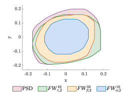
Figure 1: Feasible region of the set of $x$ and $y$ for which the $10\times 10$ $I_{10}+xA+yB$ belongs to PSD, $\mathcal{FW}^{10}_{\alpha,2}$, $\mathcal{FW}^{10}_{\beta,2}$, and $\mathcal{FW}^{10}_{\gamma,2}$, where $\alpha=\{1,1,\ldots,1\}$, $\beta=\{2,2,2,2,2\}$, $\gamma=\{4,4,2\}$.

II-C Problem statement

In [18], we have seen significant numerical efficiency improvements by approximating $\mathbb{S}^{n}_{+}$ using $DD_{n}$ and $SDD_{n}$ for solving the SDP (1), but the solution quality can be unsatisfactory. As shown in Theorem 1, the block factor-width-two matrices can improve the solution quality by using a coarser partition $\beta$ [20]. This leads to larger PSD constraints shown in (6), potentially compromising the numerical efficiency.

In this work, we aim to develop iterative inner and outer approximations for solving the SDP (1) and at each iteration the partition $\alpha$ is fixed. In this way, we solve the SDP (1) by solving smaller SDPs iteratively and maintaining the scalability at each iteration. In particular, we will combine the basis pursuit idea in [18] and the tight approximation quality of block factor-width-two matrices in [20].

III Inner approximations of the psd cone

Given a partition $\alpha$, we know $\mathcal{FW}^{n}_{\alpha,2}\subseteq\mathbb{S}^{n}_{+}\subseteq(\mathcal{FW}^{n}_{\alpha,2})^{*}$. Then, replacing $\mathbb{S}^{n}_{+}$ with $\mathcal{FW}^{n}_{\alpha,2}$ (or $(\mathcal{FW}^{n}_{\alpha,2})^{*}$, respectively) in (1) naturally gives an inner (outer, respectively) approximation for solving SDPs [20]. In this section, motivated by the basis pursuit idea in [18], we introduce an iterative algorithm for inner approximations of (1). Our algorithm returns a sequence of upper bounds with increasing accuracy.

III-A Inner Approximations

For the inner approximation, we start from replacing the PSD constraint in (1a) by $\mathcal{FW}^{n}_{\alpha,2}$, leading to

$${\mathsf{U}}_{\alpha}^{1}:=\min_{X}\quad \langle C,X\rangle$$

$$\mathrm{subject~{}to}\quad \langle A_{i},X\rangle=b_{i},\quad i=1,\ldots,m,$$ (8a)

$$X\in\mathcal{FW}^{n}_{\alpha,2},$$ (8b)

which provides an upper bound for (1a). The cyclic property of the trace operator leads to

$$\langle C,X\rangle =\left\langle C,\sum_{1\leq k<l\leq p}(E_{kl}^{\alpha})^{{\mathsf{T}}}X_{kl}E_{kl}^{\alpha}\right\rangle$$

$$=\sum_{1\leq k<l\leq p}\left\langle E_{kl}^{\alpha}C(E_{kl}^{\alpha})^{{\mathsf{T}}},X_{kl}\right\rangle.$$

This allows us to equivalently rewrite (8) into

$${\mathsf{U}}_{\alpha}^{1}:=\min_{X_{kl}} \sum_{1\leq k<l\leq p}\left\langle C_{kl},X_{kl}\right\rangle$$ (9)

$$\mathrm{subject~{}to} \sum_{1\leq k<l\leq p}\left\langle A_{i,kl},X_{kl}\right\rangle=b_{i},i=1,\ldots,m,$$

$$\;\;X_{kl}\in\mathbb{S}^{\alpha_{k}+\alpha_{l}}_{+},\qquad\quad 1\leq k<l\leq p,$$

where $C_{kl}=E_{kl}^{\alpha}C(E_{kl}^{\alpha})^{{\mathsf{T}}},A_{i,kl}=E_{kl}^{\alpha}A_{i}(E_{kl}^{\alpha})^{{\mathsf{T}}},1\leq k<l\leq p,i=1,\ldots,m$. We can now use standard conic solvers (such as SeDuMi [23] and MOSEK [7]) to solve (9). This gives an upper bound

$$d^{\star}=p^{\star}\leq{\mathsf{U}}_{\alpha}^{1}.$$ (10)

The gap ${\mathsf{U}}_{\alpha}^{1}-p^{\star}$ may be large. By Theorem 1, using a coarser partition $\alpha\sqsubseteq\beta$ can reduce the gap ${\mathsf{U}}_{\beta}^{1}-p^{\star}\leq{\mathsf{U}}_{\alpha}^{1}-p^{\star}$, but this leads to an SDP with a larger PSD constraint in (9).

We introduce another way to reduce the gap by solving a sequence of SDPs in the form of (9) while keeping the same partition $\alpha$. In particular, given an $n\times n$ matrix $V$, we define a family of cones

$$\mathcal{FW}^{n}_{\alpha,2}(V)\!\coloneqq\!\{M\in\mathbb{S}^{n}\mid M\!=\!V^{{\mathsf{T}}}QV,\,Q\!\in\!\mathcal{FW}^{n}_{\alpha,2}\}.$$ (11)

It is clear that $\mathcal{FW}^{n}_{\alpha,2}(V)=\mathcal{FW}^{n}_{\alpha,2}$ when $V=I$, and that $\mathcal{FW}^{n}_{\alpha,2}(V)$ is an inner approximation of $\mathbb{S}^{n}_{+}$ for any $V$.

When $V$ is fixed, linear optimization over $\mathcal{FW}^{n}_{\alpha,2}(V)$ amounts to solve an SDP in a similar form to (9). In particular, at each iteration $t$, we replace $\mathcal{FW}^{n}_{\alpha,2}$ in (8) with $\mathcal{FW}^{n}_{\alpha,2}(V_{t})$, and get the following problem

$${\mathsf{U}}_{\alpha}^{t}:=\min_{X_{kl}}{} \sum_{1\leq k<l\leq p}\left\langle\hat{C}_{kl},X_{kl}\right\rangle$$ (12)

$$\mathrm{subject~{}to}{} \sum_{1\leq k<l\leq p}\left\langle\hat{A}_{i,kl},X_{kl}\right\rangle=b_{i},i=1,\ldots,m$$

$$\;\;X_{kl}\in\mathbb{S}^{\alpha_{k}+\alpha_{l}}_{+},\qquad 1\leq k<l\leq p,$$

where the problem data are

$$\hat{C}_{kl} =E_{kl}^{\alpha}\left(V_{t}CV_{t}^{{\mathsf{T}}}\right)(E_{kl}^{\alpha})^{{\mathsf{T}}},$$ (13)

$$\hat{A}_{i,kl} =E_{kl}^{\alpha}\left(V_{t}A_{i}V_{t}^{{\mathsf{T}}}\right)(E_{kl}^{\alpha})^{{\mathsf{T}}},\quad 1\leq k<l\leq p.$$

We choose the sequence of matrices $\{V_{t}\}$ as

$$\begin{split}V_{1}&=I\\ V_{t+1}&=\mathrm{chol}(X_{t}^{\star}),\end{split}$$ (14)

where $\mathrm{chol}(\cdot)$ denotes a Cholesky factorization, and $X_{t}^{\star}:=\sum_{1\leq k<l\leq p}V_{t}^{{\mathsf{T}}}(E_{kl}^{\alpha})^{{\mathsf{T}}}X_{kl}^{t,\star}E_{kl}^{\alpha}V_{t}$ is the optimal solution to (12) at iteration $t$. When choosing $V_{1}=I$ at iteration 1, problem (12) reduces to (9).

III-B Monotonically decreasing upper bounds

The choice of the matrices $V_{t+1}$ as the factorization of $X_{t}^{\star}$ in (14) leads to a sequence of monotonically decreasing cost values in (12). We have the following proposition.

Proposition 1

Given any partition $\alpha$, solving (12) with matrices $\{V_{t}\}$ in (14) leads to

$${\mathsf{U}}^{1}_{\alpha}\geq{\mathsf{U}}^{2}_{\alpha}\geq\ldots\geq{\mathsf{U}}^{t}_{\alpha}\geq{\mathsf{U}}^{t+1}_{\alpha}\geq p^{\star}.$$

Proof:

Upon choosing $V_{t+1}=\mathrm{chol}(X_{t}^{\star})$, we naturally have $X_{t}=V_{t+1}^{{\mathsf{T}}}\times I\times V_{t+1}$. Since $I\in\mathcal{FW}^{n}_{\alpha,2}$, we have $X_{t}^{\star}\in\mathcal{FW}^{n}_{\alpha,2}(V_{t+1})$. It means that the optimal solution $X_{t}^{\star}$ at iteration $t$ is in the feasible region of the SDP at iteration $t+1$. Thus, we have ${\mathsf{U}}^{t}_{\alpha}\geq{\mathsf{U}}^{t+1}_{\alpha}$. ∎

Input: SDP data $A_{i},C\in\mathbb{S}^{n},b\in\mathbb{R}^{m}$, block partition $\alpha$, and maximum iteration $t_{\max}$

Output: Upper bound ${\mathsf{U}}_{\alpha}$

Initialize $t=1;$ $V_{1}=I;$

while $t<t_{\max}$  do

       Solve (12) to get ${\mathsf{U}}_{\alpha}^{t}$ and $X_{kl}^{t,\star},1\leq k<l\leq p;$

       Set ${\mathsf{U}}_{\alpha}={\mathsf{U}}_{\alpha}^{t};$

       Compute

$$X_{t}^{\star}=\sum_{1\leq k<l\leq p}V_{t}^{{\mathsf{T}}}(E_{kl}^{\alpha})^{{\mathsf{T}}}X_{kl}^{t,\star}E_{kl}^{\alpha}V_{t};$$

$$V_{t+1}=\mathrm{chol}(X_{t}^{\star});$$

       Update $\hat{C}_{kl},\hat{A}_{i,kl}$ as (13); Set $t=t+1;$

end while

return ${\mathsf{U}}_{\alpha}$

Algorithm 1 Inner-approximations using $\mathcal{FW}^{n}_{\alpha,2}$

When $X_{t}^{\star}$ is positive definite, we have a strictly decreasing cost value, as summarized in the following theorem.

Theorem 2

Given any partition $\alpha$, let $X_{t}^{\star}$ be an optimal solution of (12) at iterate $t$. If $X_{t}^{\star}$ is positive definite and ${\mathsf{U}}^{t}_{\alpha}>p^{\star}$, then ${\mathsf{U}}^{t}_{\alpha}>{\mathsf{U}}^{t+1}_{\alpha}\geq p^{\star}$.

Proof:

Let $X^{\star}$ and $p^{\star}$ be the optimal solution and cost value of (1). We construct a point

$$\hat{X}\coloneqq(1-\lambda)X_{t}^{\star}+\lambda X^{\star},$$ (15)

with some $\lambda\in(0,1)$. We will prove there exists a $\lambda\in(0,1)$ such that $\hat{X}$ in (15) is feasible for (12) at iteration $t+1$. Therefore, we complete the proof by observing

$$U^{t+1}_{\alpha}\leq\langle C,\hat{X}\rangle=(1-\lambda)\langle C,X_{t}^{\star}\rangle+\lambda\langle C,X^{\star}\rangle<U^{t}_{\alpha}.$$

To prove $\hat{X}$ is feasible at iteration $t+1$ for some $\lambda\in(0,1)$, we need to show $\hat{X}$ satisfies

• the linear constraint (8a),

• the conic constraint (8b) with $\mathcal{FW}^{n}_{\alpha,2}(V_{t+1})$.

First, it is clear that both $X_{t}^{\star}$ and $X^{\star}$ satisfy (8a), i.e.,

$$\langle A_{i},X_{t}^{\star}\rangle =b_{i},\;\;i=1,\ldots,m,$$

$$\langle A_{i},X^{\star}\rangle =b_{i},\;\;i=1,\ldots,m.$$

Then, we have $\forall i=1,\ldots,m$,

$$\left\langle A_{i},\hat{X}\right\rangle =\langle A_{i},(1-\lambda)X_{t}^{\star}+\lambda X^{\star}\rangle$$

$$=(1-\lambda)\langle A_{i},X_{t}^{\star}\rangle+\lambda\langle A_{i},X^{\star}\rangle=b_{i}.$$

Since $X_{t}^{\star}=V_{t+1}^{{\mathsf{T}}}V_{t+1}$ and $X_{t}^{\star}$ is positive definite, $V_{t+1}$ must be invertible. We let

$$\tilde{X}_{t+1}\coloneqq\left(V_{t+1}^{-1}\right)^{{{\mathsf{T}}}}X^{\star}V_{t+1}^{-1}.$$

Then, for small enough $\lambda>0$, the matrix $(1-\lambda)I+\lambda\tilde{X}_{t+1}\in\mathcal{FW}^{n}_{\alpha,2}$. Hence, from (15), we have

$$\hat{X}=V^{{{\mathsf{T}}}}_{t+1}((1-\lambda)I+\lambda\tilde{X}_{t+1})V_{t+1}\in\mathcal{FW}^{n}_{\alpha,2}(V_{t+1}).$$

This completes the proof. ∎

Our proof is inspired by [18, Theorem 3.1], and we generalize it to any block partition $\alpha$, including the iterative algorithm based on SDD matrices [18, Section 4] as a special case. The key idea is to make sure the optimal solution of the previous iteration is a feasible point in the next iteration. Thus, instead of the Cholesky decomposition, we can use other choices, such as spectral decomposition $X_{t}^{\star}=PDP^{{\mathsf{T}}}$.

Algorithm 1 lists the overall procedure of the proposed iterative inner approximations for solving (1). We use a simple example to illustrate our algorithm.

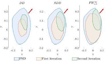
Figure 2: Feasible regions of inner approximations of (16) in Algorithm 1 using $DD$, $SDD$, and $\mathcal{FW}^{n}_{\alpha,2}$ with $\alpha=\{2,2,2,2,2\}$. The red arrows denote the decreasing direction of the cost value.

TABLE I: Cost values of inner approximations in Algorithm 1 for solving (16). We used $DD$, $SDD$, and $\mathcal{FW}^{n}_{\alpha,2}$ with $\alpha=\{2,2,2,2,2\}$. The optimal cost of (16) is $-0.298$.

	DD		SDD		$\mathcal{FW}^{n}_{\alpha,2}$
Iter	Cost	Gap	Cost	Gap	Cost	Gap
$1$	$-0.148$	$50.3$%	$-0.176$	$40.9$%	$-0.232$	$22.2$%
$2$	$-0.236$	$20.8$%	$-0.277$	$7.04$%	$-0.298$	$0$%

Example 1

Consider an SDP of the form

$$\min_{x,y} -x-y$$ (16)

$$\mathrm{subject~{}to} I+xA+yB\succeq 0,$$

where $A$ and $B$ are two $10\times 10$ matrices with each entry randomly generated. We consider inner approximations by DD, SDD and $\mathcal{FW}_{\alpha}^{10}$ with $\alpha=\{2,2,2,2,2\}$. The results are shown in Figure 2. The blue part in Figure 2 shows the feasible region of (16). We then replace the semidefinite constraint by $DD$, $SDD$ and $\mathcal{FW}^{10}_{\alpha,2}$. Orange and green parts in Figure 2 show the feasible regions in iteration 1 and 2 of Algorithm 1. It is clear that the feasible region moves towards the direction where the cost decreases. As shown in Table I (also in Figure 2), our algorithm using $\mathcal{FW}^{n}_{\alpha,2}$ achieves the optimal cost at the second iteration, while the results from DD/SDD approximations [18] are still far away from the optimal cost. $\square$

IV Outer Approximations of the PSD cone

The inner approximation in (8) provides an upper bound of the SDPs (1). Here, we introduce an outer approximation for the same problem (1a), which provides a lower bound. Therefore, the optimal cost of (1) can be bounded above and below simultaneously.

IV-A Outer approximations

Consider the relationship $\mathcal{FW}^{n}_{\alpha,2}\subseteq\mathbb{S}^{n}_{+}\subseteq(\mathcal{FW}^{n}_{\alpha,2})^{*}$. Replacing PSD cone $\mathbb{S}^{n}_{+}$ by the dual cone $(\mathcal{FW}^{n}_{\alpha,2})^{*}$ gives an outer approximation of (1a), i.e.,

$${\mathsf{L}}_{\alpha}^{1}\coloneqq\min_{X} \langle C,X\rangle$$ (17)

$$\mathrm{subject~{}to} \langle A_{i},X\rangle=b_{i},\qquad i=1,\ldots,m,$$

$$X\in(\mathcal{FW}^{n}_{\alpha,2})^{*}.$$

We have ${\mathsf{L}}_{\alpha}^{1}\leq d^{\star}=p^{\star}.$ Note that the dual cone $(\mathcal{FW}^{n}_{\alpha,2})^{*}$ admits a decomposition as [20]

$$(\mathcal{FW}^{n}_{\alpha,2})^{*}=\Big{\{}X\in\mathbb{S}^{n}\mid E_{kl}^{\alpha}X(E_{kl}^{\alpha})^{{\mathsf{T}}}\in\mathbb{S}^{\alpha_{k}+\alpha_{l}}_{+},$$ (18)

$$\qquad\qquad 1\leq k<l\leq p\Big{\}}.$$

Therefore, problem (17) can be rewritten as:

$${\mathsf{L}}_{\alpha}^{1}=\min_{X} \langle C,X\rangle$$ (19)

$$\mathrm{subject~{}to} \langle A_{i},X\rangle=b_{i},\qquad i=1,\ldots,m,$$

$$E_{kl}^{\alpha}X(E_{kl}^{\alpha})^{{\mathsf{T}}}\in\mathbb{S}^{\alpha_{k}+\alpha_{l}}_{+},1\leq k<l\leq p.$$

The gap $p^{\star}-{\mathsf{L}}_{\alpha}^{1}$ might be large. Similar to inner approximations, we aim to solve a sequence of outer approximations in the following form

$${\mathsf{L}}_{\alpha}^{t}\coloneqq\min_{X}\quad \langle C,X\rangle$$

$$\mathrm{subject~{}to}\quad \langle A_{i},X\rangle=b_{i},\qquad i=1,\ldots,m,$$ (20)

$$E_{kl}^{\alpha}V_{t}XV_{t}^{{\mathsf{T}}}(E_{kl}^{\alpha})^{{\mathsf{T}}}\in\mathbb{S}^{\alpha_{k}+\alpha_{l}}_{+},1\leq k<l\leq p,$$

which is parameterized by $V_{t}\in\mathbb{R}^{n\times n}$. However, we cannot generate the matrix $V_{t+1}$ by Cholesky decomposition of the optimal solution $X_{t}$ of (20), since it is not positive semidefinite. To resolve this, motivated by [18], we look into the dual problem of (20), which is

$${\mathsf{L}}_{\alpha}^{t}=\max_{y,X_{kl}}\quad b^{{\mathsf{T}}}y$$

$$\mathrm{subject~{}to}\quad C-\sum_{i=1}^{m}y_{i}A_{i}=\sum_{1\leq k<l\leq p}V_{t}^{{\mathsf{T}}}(E_{kl}^{\alpha})^{{\mathsf{T}}}X_{kl}E_{kl}^{\alpha}V_{t},$$

$$X_{kl}\in\mathbb{S}^{\alpha_{k}+\alpha_{l}}_{+},\quad 1\leq k<l\leq p.$$ (21)

For the optimal solution $y^{t,\star}$ of (21) at iteration $t$, the matrix $C-\sum_{i=1}^{m}y_{i}^{t,\star}A_{i}$ is guaranteed to be positive semidefinite. Then, we choose a sequence of matrices $\{V_{t}\}$ for (21) as

$$\begin{split}V_{1}&=I\\ V_{t+1}&=\mathrm{chol}\left(C-\sum_{i=1}^{m}y_{i}^{t,\star}A_{i}\right),\end{split}$$ (22)

where $y^{t,\star}$ is the optimal solution of (21) at iteration $t$.

IV-B Monotonically increasing lower bounds

The lower bounds from the sequence of outer approximations defined in (21) and (22) are monotonically increasing, as proved in the following result.

Proposition 2

Given any partition $\alpha$, solving (21) with matrices $\{V_{t}\}$ in (22) leads to

$${\mathsf{L}}^{1}_{\alpha}\leq{\mathsf{L}}^{2}_{\alpha}\leq\ldots\leq{\mathsf{L}}^{t}_{\alpha}\leq{\mathsf{L}}^{t+1}_{\alpha}\leq d^{\star}=p^{\star}.$$

Proof:

It is not difficult to see that the dual problem (21) is equivalent to

$$\max_{y}\quad b^{{\mathsf{T}}}y$$

$$\mathrm{subject~{}to}\quad C-\sum_{i=1}^{m}y_{i}A_{i}\in\mathcal{FW}^{n}_{\alpha,2}(V_{t}).$$ (23)

Suppose the optimal solution to (23) at iteration $t$ is $y_{i}^{t,\star}$. Let

$$Z_{t}^{\star}=C-\sum_{i=1}^{m}y_{i}^{t,\star}A_{i},\quad V_{t+1}=\mathrm{chol}(Z_{t}^{\star}).$$

We have $Z_{t}^{\star}=V_{t+1}^{{\mathsf{T}}}\times I\times V_{t+1}\in\mathcal{FW}^{n}_{\alpha,2}(V_{t+1})$ since $I\in\mathcal{FW}^{n}_{\alpha,2}$. It means that $y_{i}^{t,\star}$ is feasible to (23) at iteration $t+1$. Thus, we have ${\mathsf{L}}^{t}_{\alpha}\leq{\mathsf{L}}^{t+1}_{\alpha}$. ∎

Similar to Theorem 2, when $C-\sum_{i=1}^{m}y_{i}^{t,\star}A_{i}$ is strictly positive definite, we have a strictly increasing cost, as summarized in the following theorem.

Theorem 3

Given any partition $\alpha$, let $\{y_{i}^{t,\star},X_{kl}^{t,\star}\}$ be an optimal solution of (21) at iterate $t$. If $C-\sum_{i=1}^{m}y_{i}^{t,\star}A_{i}$ is strictly positive definite and ${\mathsf{L}}^{t}_{\alpha}<d^{\star}$, then ${\mathsf{L}}^{t}_{\alpha}<{\mathsf{L}}^{t+1}_{\alpha}\leq d^{\star}$.

Proof:

Let $({y^{\star},Z^{\star}})$ be the optimal solution of (1b), and $y_{i}^{t,\star}$ is an optimal solution of (23) at iteration $t$. We construct

$$\hat{y}\coloneqq(1-\lambda)y^{t,\star}+\lambda y^{\star},$$ (24)

with some $\lambda\in(0,1)$. We will prove there exists a $\lambda\in(0,1)$ such that $\hat{y}$ in (24) is feasible for (23) at iteration $t+1$. We then complete the proof by observing

$${\mathsf{L}}^{t+1}_{\alpha}=b^{{\mathsf{T}}}y^{t+1,\star}\geq b^{{\mathsf{T}}}\hat{y}=(1-\lambda)b^{{\mathsf{T}}}y^{t,\star}+\lambda b^{{\mathsf{T}}}y^{\star}>{\mathsf{L}}^{t}_{\alpha}.$$

To prove $\hat{y}$ is feasible at iteration $t+1$, we need to show

$$C-\sum_{i=1}^{m}\hat{y}_{i}A_{i}\in\mathcal{FW}^{n}_{\alpha,2}(V_{t+1}),\;\text{for some}\;\lambda\in(0,1).$$ (25)

Indeed, we have

$$C-\sum_{i=1}^{m}\hat{y}_{i}A_{i}$$

$$= (1-\lambda)\left(C-\sum_{i=1}^{m}y^{t,\star}_{i}A_{i}\right)+\lambda\left(C-\sum_{i=1}^{m}y^{\star}_{i}A_{i}\right).$$

Since $C-\sum_{i=1}^{m}y^{t,\star}_{i}A_{i}=V_{t+1}^{{\mathsf{T}}}V_{t+1}$ that is strictly positive definite, $V_{t+1}$ must be invertible. Then, we have

$$\left(V_{t+1}^{-1}\right)^{{{\mathsf{T}}}}\left(C-\sum_{i=1}^{m}\hat{y}_{i}A_{i}\right)V_{t+1}^{-1}$$

$$= (1-\lambda)I+\lambda\left(V_{t+1}^{-1}\right)^{{{\mathsf{T}}}}\left(C-\sum_{i=1}^{m}y^{\star}_{i}A_{i}\right)V_{t+1}^{-1}\in\mathcal{FW}^{n}_{\alpha}$$

when $\lambda\in(0,1)$ is small enough. It means that (25) holds with this $\lambda$ for $\hat{y}$ in (24). This completes the proof. ∎

Input: SDP data $A_{i},C\in\mathbb{S}^{n},b\in\mathbb{R}^{m}$, block partition $\alpha$, and maximum iteration $t_{\max}$

Output: Lower bound ${\mathsf{L}}_{\alpha}$

Initialize $t=1;V_{1}=I;$

while $t<t_{\max}$  do

       Solve $\eqref{eq:outer-approximation-step-t-dual}$ to get ${\mathsf{L}}_{\alpha}^{t}$ and $y^{t,\star};$

      Set ${\mathsf{L}}_{\alpha}={\mathsf{L}}_{\alpha}^{t};$

       Compute $V_{t+1}=\mathrm{chol}(C-\sum_{i=1}^{m}y_{i}^{t,\star}A_{i});$

       Set $t=t+1;\;$

end while

return ${\mathsf{L}}_{\alpha}$

Algorithm 2 Outer-approximations using $\mathcal{FW}^{n}_{\alpha,2}$

Remark 1 (Solving outer approximations)

Unlike the inner approximations (12), the outer approximations (20) and (21) are not in the standard form of SDPs. Thus they cannot be solved directly using standard conic solvers. In our implementation, we apply the idea in [24] and transform (21) into the following primal form of SDPs

$$\min_{y,X_{kl}}\; -b^{{\mathsf{T}}}y$$

$$\mathrm{subject~{}to}\; \sum_{1\leq k<l\leq p}V_{t}^{{\mathsf{T}}}(E_{kl}^{\alpha})^{{\mathsf{T}}}X_{kl}E_{kl}^{\alpha}V_{t}+\sum_{i=1}^{m}y_{i}A_{i}=C,$$

$$X_{kl}\in\mathbb{S}^{\alpha_{k}+\alpha_{l}}_{+},1\leq k<l\leq p,$$ (26)

which is ready to be solved using standard conic solvers. We note that the size of PSD constraints has been reduced in (23), but the number of equality constraints is $n^{2}$. Thus, solving (23) might not be as efficient as solving (12). $\square$

Our iterative outer approximations for solving (1) is listed in Algorithm 2. We use SDP (16) to illustrate our algorithm.

Example 2

The feasible regions in the first and $11$th iterations are shown in Figure 3. In particular, the blue part shows the feasible region of (16). We then replace the PSD constraint by $(DD)^{*}$, $(SDD)^{*}$ and $(\mathcal{FW}^{10}_{\alpha,2})^{*}$. Orange and green regions are the feasible regions in iterations 1 and 11. It is clear that the feasible region moves towards the direction where the cost increases. As shown in Table II (also in Figure 3), our algorithm using $\mathcal{FW}^{n}_{\alpha,2}$ achieves the optimal cost at iteration 11, while the results from DD/SDD approximations [18] are still far away from the optimal cost. $\square$

Figure 4 shows the convergence of the upper and lower bounds of SDP (16) from Algorithm 1 and 2. In this case, the convergence using $\mathcal{FW}^{n}_{\alpha,2}$ is much faster than the DD/SDD strategies [14, 18].

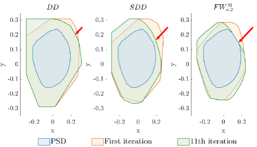
Figure 3: Feasible regions of outer approximations in Algorithm 2 by $DD$, $SDD$, and $\mathcal{FW}^{n}_{\alpha,2}$ with $\alpha=\{2,2,2,2,2\}$. The red arrow denotes the increasing direction of the cost value.

TABLE II: Cost values of iteratively outer approximation (16) using $DD$, $SDD$, and $\mathcal{FW}^{n}_{\alpha,2}$. The optimal cost value of (16) is $-0.298$.

	DD		SDD		$\mathcal{FW}^{n}_{\alpha,2}$
Iter	Cost	Gap	Cost	Gap	Cost	Gap
$1$	$-0.499$	$67.5$%	$-0.469$	$57.4$%	$-0.401$	$34.6$%
$11$	$-0.443$	$48.7$%	$-0.350$	$17.6$%	$-0.298$	$0$%

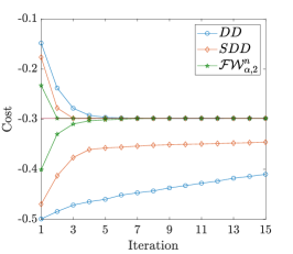
Figure 4: Inner/Outer approximations of SDP (16) using DD, SDD, and $\mathcal{FW}^{n}_{2,\alpha}$ with $\alpha=\{2,\ldots,2\}$.

Remark 2 (Role of partition $\alpha$)

In our Algorithms 1-2, the choice of partition $\alpha$ brings flexibility in balancing the computational efficiency and solution quality at each iteration. Choosing a suitable partition might be problem dependent; we refer interested readers to [20] for more discussions. Here, we highlight that 1) a coarser partition normally leads to faster convergence in Algorithms 1-2, as shown in our extensive numerical experiments in Section V; 2) a coarser partition also leads to a smaller number $p$ in (21) and (12). The latter fact is important in constructing the problem in each iteration, especially for large-scale cases. For example, when $n=2000$, if we use the SDD matrices for inner/outer approximations [14, 18], the number of small blocks is $\binom{2000}{2}=1\,999\,000$ which is too large to even construct the problem instances (21) and (12). We indeed failed to construct such problems in our experiments in Section V-C. Instead, for $\alpha=\{10,\ldots,10\}$ ($\beta=\{20,\ldots,20\}$, respectively), the number of blocks is reduced to $\binom{200}{2}=19900$ ($\binom{100}{2}=4950$, respectively), for which efficient constructions exist.

V Numerical Results

In this section, we present computational results of Algorithms 1-2 on three classes of SDPs: 1) independent stable set, 2) binary quadratic optimization, and 3) SDPs with random data. Our experiments were carried out in MATLAB R2021a on a Windows PC with 2.6 GHz speed and 24 GB RAM. All the SDP instances at each iteration of Algorithms 1-2 were solved by MOSEK [7].

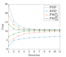
Figure 5: Inner/Outer approximations of Lov$\acute{a}$sz theta number (28) by different partitions: $\alpha=\{2,\ldots,2\}$, and $\beta=\{5,\ldots,5\}$.

TABLE III: Success rate of upper bounds of $\vartheta(\mathcal{G})$ in (28) for $140$ instances of 30-nodes Erd$\ddot{o}$s-$\acute{R}$enyi graphs using Algorithm 2, where $\alpha=\{2,\ldots,2\}$ and $\beta=\{5,\ldots,5\}$.

Iteration $t$	SDD	$\mathcal{FW}^{n}_{\alpha,2}$	$\mathcal{FW}^{n}_{\beta,2}$
$1$	$0\%$	$0\%$	$0\%$
$3$	$0\%$	$5.7\%$	$36.4\%$
$5$	$20\%$	$36.4\%$	$86.4\%$
$7$	$35.7\%$	$79.3\%$	$95.7\%$

V-A The maximum stable set problem

The maximum stable set problem is a classical combinatorial problem, which aims to find the stability number of a graph. A stable set of a undirected graph $\mathcal{G}=(\mathcal{V},\mathcal{E})$ is a set of nodes of $\mathcal{G}$ such that there are no edges between them. The maximum stable number of $\mathcal{G}$, denoted as $\alpha(\mathcal{G})$, is the size of maximum stable set. However, testing whether a $\alpha(\mathcal{G})$ is greater than an integer $k$ is well-known to be NP-complete [25]. This problem can be formulated as

$$\alpha(\mathcal{G})\coloneqq\max_{x_{i}} \sum_{i=1}^{n}x_{i}$$ (27)

$$\mathrm{subject~{}to} x_{i}\in\{0,1\},\quad i=1,2,\ldots,n,$$

$$x_{i}x_{j}=0,\quad\forall(i,j)\in\mathcal{E}.$$

A well-known SDP-based upper bound, introduced in [26], can be computed by

$$\vartheta(\mathcal{G})\coloneqq\max_{X} \langle J,X\rangle$$ (28)

$$\mathrm{subject~{}to} \langle I,X\rangle=1,$$

$$X_{ij}=0,\quad\forall(i,j)\in\mathcal{E},$$

$$X\succeq 0,$$

where $J$ is an all-one matrix and $I$ is the identity matrix. The cost of (28) is called Lov$\acute{a}$sz theta number, denoted as $\vartheta(\mathcal{G})$, which provides an upper bound $\vartheta(\mathcal{G})\geq\alpha(\mathcal{G})$. We now apply Algorithms 1 and 2 to get a sequence of upper and lower bounds on Lov$\acute{a}$sz theta number.

We first generated a Erd$\ddot{o}$s-$\acute{R}$enyi graph of 30 nodes with edge probability 0.2, and then applied Algorithms 1 and 2 using three different partitions: SDD (trivial partition), $\alpha=\{2,\ldots,2\}$, and $\beta=\{5,\ldots,5\}$. As shown in Figure 5, a coarser partition $\beta$ leads to the fastest convergence for both inner and outer approximation in this case. To give a more quantitative comparison, we further generated 140 instances of 30-node Erd$\ddot{o}$s-$\acute{R}$enyi graphs with edge probability from 0.2 to 0.8. We use Algorithm 2 to compute the upper bound of $\vartheta(\mathcal{G})$. When the upper bound is within 99% suboptimality to $\vartheta(\mathcal{G})$, we consider it as a success. Table III lists the success rate at different iterations of Algorithm 2. As expected, a coarser partition $\beta$ gives much higher success rates compared to SDD approximation [18]. Specifically, in the seventh iteration, $\mathcal{FW}^{n}_{\beta,2}$ obtains $95.7\%$ success rate, while SDD only has $35.7\%$ success rate.

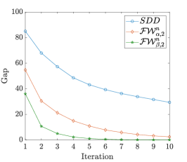
Figure 6: Inner approximation on the binary quadratic optimization (30) with $\alpha=\{10,\ldots,10\}$ and $\beta=\{20,\ldots,20\}$.

TABLE IV: Upper bounds of (30) at iteration 10 using SDD, $\mathcal{FW}^{n}_{\alpha,2}$, $\mathcal{FW}^{n}_{\beta,2}$ with $\alpha=\{10,\ldots,10\},~{}\beta=\{20,\ldots,20\}$.

	SDD		$\mathcal{FW}^{n}_{\alpha,2}$		$\mathcal{FW}^{n}_{\beta,2}$
Instance	Gap	Time	Gap	Time	Gap	Time
1	$28.77$	$43.5$	$3.02$	$27.0$	$0.05$	$32.4$
2	$30.81$	$51.4$	$2.31$	$25.6$	$0.03$	$30.4$
3	$29.24$	$48.4$	$3.54$	$27.5$	$0.04$	$29.2$
4	$29.45$	$47.2$	$3.14$	$26.5$	$0.04$	$32.7$
5	$29.40$	$55.8$	$2.43$	$26.7$	$0.03$	$36.9$

V-B Binary quadratic optimization

Binary quadratic optimization is another classical combinatorial problem, in which we have a quadratic cost and a binary decision variable $x$. Formally, the problem is

$$\min_{x} x^{T}Qx$$ (29)

$$\mathrm{subject~{}to} x_{i}^{2}=1,\quad i=1,2,\ldots,n,$$

where $Q\in\mathbb{S}^{n}$. Many well-known problems are in the form of (29), such as max-cut problems [27]. The quadratic constraint define a finite set. The number of elements grows with the rate $2^{n}$. It is well-known that such a problem is NP-complete [28]. A standard semidefinite relaxation is

$$\min_{X} \langle Q,X\rangle$$ (30)

$$\mathrm{subject~{}to} X_{ii}=1,\quad i=1,2,\ldots,n,$$

$$X\in\mathbb{S}^{n}_{+},$$

which returns a lower bound for (29).

We apply Algorithm 1 for inner approximations of (30). We generated five random cost matrices $Q\in\mathbb{S}^{100}$. We apply three different partitions: SDD, $\alpha=\{10,\ldots,10\}$, and $\beta=\{20,\ldots,20\}$. We set the maximum iteration as $10$. The results are shown in Figure 6 and Table IV. As expected again, as the partition becomes coarser, the approximation quality increases. For example, inner approximation by partition $\beta$ obtains almost optimal solution ($\geq 99.9\%$ optimality) within $10$ iterations, while SDD can only achieve around $70\%$ optimality while taking a longer time (the longer time consumption is related to the large number of small blocks; see Remark 2).

V-C Random SDPs

Our final experiment is to show the scalability of the inner approximations in Algorithm 1. We generated seven random large-scale SDPs with PSD constraints of $1500$, $2000$, $2500$, $3000$, $3500$, $4000$, and $4500$. The number of linear constraints is fixed as $m=10$. We approximate the PSD cone using two different partitions $\alpha=\{10,\ldots,10\}$ and $\beta=\{20,\ldots,20\}$. As discussed in Remark 2, we failed to use SDD approximation in this large-scale experiment.

We ran Algorithm 1 for 30 minutes and then compare the solution quality. The optimality gap is computed by $\lvert\frac{p^{\star}-f_{30}}{p^{\star}}\rvert\times 100\%$, where $p^{\star}$ is the optimal cost value of original SDP, and $f_{30}$ is the obtained upper bound after running $30$ minutes. The results are listed in Table V. Our proposed method shows promising efficiency and accuracy. For example, when $n=4500$ and $m=10$, Algorithm 1 with partition $\beta$ obtained a solution with $99.9\%$ optimality in $30$ minutes, while original SDP took over 4.5 hours to solve.

TABLE V: Computational results of 6 different large-scale SDPs using Algorithm 1 with $\alpha=\{10,\ldots,10\}$ and $\beta=\{20,\ldots,20\}$. $f_{1}$ denotes the cost value of the first iteration. $f_{30}$ denotes the cost value after $30$ minutes. The time consumption (in seconds) for solving the original SDP is listed in the last column.

	$\mathcal{FW}^{n}_{\alpha,2}$			$\mathcal{FW}^{n}_{\beta,2}$			PSD
$n$	$f_{1}$	$f_{30}$	Gap	$f_{1}$	$f_{30}$	Gap	Time
$1500$	$5.63e6$	$4.76e6$	$0.03$	$5.20e6$	$4.76e6$	$0.03$	$603$
$2000$	$3.33e6$	$2.86e6$	$0.10$	$3.09e6$	$2.86e6$	$0.05$	$1\,201$
$2500$	$6.11e6$	$5.29e6$	$0.07$	$5.70e6$	$5.29e6$	$0.05$	$2\,893$
$3000$	$1.81e7$	$1.32e7$	$0.79$	$1.57e7$	$1.32e7$	$0.79$	$5\,508$
$3500$	$8.96e6$	$7.08e6$	$0.10$	$8.02e6$	$7.07e6$	$0.08$	$7\,369$
$4000$	$9.52e6$	$6.89e6$	$0.15$	$8.21e6$	$6.89e6$	$0.11$	$10\,689$
$4500$	$2.05e7$	$1.70e7$	$0.08$	$1.88e7$	$1.69e7$	$0.06$	$16\,989$

VI Conclusions

In this paper, we have introduced the iterative inner/outer approximations for solving SDPs (cf. Algorithm 1-2), and analyzed their solution quality (cf. Propositions 1-2 and Theorems 2-3). Numerical results on stable set, binary quadratic optimization, and random SDPs have shown promising accuracy and computational scalability when proper partitions were used. Future work includes analyzing the convergence of (or modified) Algorithm 1-2 (some recent results appeared in [19]). Developing other types of iterative algorithms based on block factor-width matrices will also be interesting.

References

- [1] S. Boyd, L. El Ghaoui, E. Feron, and V. Balakrishnan, Linear matrix inequalities in system and control theory. SIAM, 1994.
- [2] R. Sotirov, “SDP relaxations for some combinatorial optimization problems,” in Handbook on Semidefinite, Conic and Polynomial Optimization. Springer, 2012, pp. 795–819.
- [3] G. Blekherman, P. A. Parrilo, and R. R. Thomas, Semidefinite optimization and convex algebraic geometry. SIAM, 2012.
- [4] L. Vandenberghe and S. Boyd, “Semidefinite programming,” SIAM review, vol. 38, no. 1, pp. 49–95, 1996.
- [5] Y. Zheng, G. Fantuzzi, and A. Papachristodoulou, “Chordal and factor-width decompositions for scalable semidefinite and polynomial optimization,” Annual Reviews in Control, vol. 52, pp. 243–279, 2021.
- [6] A. Majumdar, G. Hall, and A. A. Ahmadi, “Recent scalability improvements for semidefinite programming with applications in machine learning, control, and robotics,” Annual Review of Control, Robotics, and Autonomous Systems, vol. 3, pp. 331–360, 2020.
- [7] M. ApS, “Mosek optimization toolbox for matlab,” User’s Guide and Reference Manual, Version, vol. 4, 2019.
- [8] B. O’donoghue, E. Chu, N. Parikh, and S. Boyd, “Conic optimization via operator splitting and homogeneous self-dual embedding,” Journal of Optimization Theory and Applications, vol. 169, no. 3, pp. 1042–1068, 2016.
- [9] Y. Zheng, G. Fantuzzi, A. Papachristodoulou, P. Goulart, and A. Wynn, “Chordal decomposition in operator-splitting methods for sparse semidefinite programs,” Mathematical Programming, vol. 180, no. 1, pp. 489–532, 2020.
- [10] ——, “CDCS: Cone decomposition conic solver, version 1.1,” 2016.
- [11] L. Vandenberghe and M. S. Andersen, “Chordal graphs and semidefinite optimization,” Foundations and Trends in Optimization, vol. 1, no. 4, pp. 241–433, 2015.
- [12] Y. Zheng and G. Fantuzzi, “Sum-of-squares chordal decomposition of polynomial matrix inequalities,” Math. Program., pp. 1–38, 2021.
- [13] E. G. Boman, D. Chen, O. Parekh, and S. Toledo, “On factor width and symmetric H-matrices,” Linear algebra and its applications, vol. 405, pp. 239–248, 2005.
- [14] A. A. Ahmadi and A. Majumdar, “DSOS and SDSOS optimization: more tractable alternatives to sum of squares and semidefinite optimization,” SIAM J Appl Math., vol. 3, no. 2, pp. 193–230, 2019.
- [15] D. Bertsimas and R. Cory-Wright, “On polyhedral and second-order cone decompositions of semidefinite optimization problems,” Operations Research Letters, vol. 48, no. 1, pp. 78–85, 2020.
- [16] A. A. Ahmadi, S. Dash, and G. Hall, “Optimization over structured subsets of positive semidefinite matrices via column generation,” Discrete Optimization, vol. 24, pp. 129–151, 2017.
- [17] Y. Wang, A. Tanaka, and A. Yoshise, “Polyhedral approximations of the semidefinite cone and their application,” Computational Optimization and Applications, vol. 78, no. 3, pp. 893–913, 2021.
- [18] A. A. Ahmadi and G. Hall, “Sum of squares basis pursuit with linear and second order cone programming,” Algebraic and geometric methods in discrete mathematics, vol. 685, pp. 27–53, 2017.
- [19] B. Roig-Solvas and M. Sznaier, “A globally convergent lp and socp-based algorithm for semidefinite programming,” arXiv preprint arXiv:2202.12374, 2022.
- [20] Y. Zheng, A. Sootla, and A. Papachristodoulou, “Block factor-width-two matrices and their applications to semidefinite and sum-of-squares optimization,” IEEE Transactions on Automatic Control, 2022.
- [21] A. Sootla, Y. Zheng, and A. Papachristodoulou, “Block factor-width-two matrices in semidefinite programming,” in 2019 18th European Control Conference (ECC). IEEE, 2019, pp. 1981–1986.
- [22] F. Alizadeh and D. Goldfarb, “Second-order cone programming,” Mathematical programming, vol. 95, no. 1, pp. 3–51, 2003.
- [23] J. F. Sturm, “Using sedumi 1.02, a matlab toolbox for optimization over symmetric cones,” Optimization methods and software, vol. 11, no. 1-4, pp. 625–653, 1999.
- [24] J. Löfberg, “Dualize it: software for automatic primal and dual conversions of conic programs,” Optimization Methods & Software, vol. 24, no. 3, pp. 313–325, 2009.
- [25] R. M. Karp, “Reducibility among combinatorial problems,” in Complexity of computer computations. Springer, 1972, pp. 85–103.
- [26] L. Lovász, “On the shannon capacity of a graph,” IEEE Transactions on Information theory, vol. 25, no. 1, pp. 1–7, 1979.
- [27] P. Festa, P. M. Pardalos, M. G. Resende, and C. C. Ribeiro, “Randomized heuristics for the max-cut problem,” Optimization methods and software, vol. 17, no. 6, pp. 1033–1058, 2002.
- [28] J. Hartmanis, “Computers and intractability: a guide to the theory of np-completeness (michael r. garey and david s. johnson),” Siam Review, vol. 24, no. 1, p. 90, 1982.