GM-TOuNN: Graded Multiscale Topology Optimization using Neural Networks

Abstract

Multiscale topology optimization (M-TO) entails generating an optimal global topology, and an optimal set of microstructures at a smaller scale, for a physics-constrained problem. With the advent of additive manufacturing, M-TO has gained significant prominence. However, generating optimal microstructures at various locations can be computationally very expensive. As an alternate, graded multiscale topology optimization (GM-TO) has been proposed where one or more pre-selected and graded (parameterized) microstructural topologies are used to fill the domain optimally. This leads to a significant reduction in computation while retaining many of the benefits of M-TO.

A successful GM-TO framework must: (1) be capable of efficiently handling numerous pre-selected microstructures, (2) be able to continuously switch between these microstructures during optimization, (3) ensure that the partition of unity is satisfied, and (4) discourage microstructure mixing at termination.

In this paper, we propose to meet these requirements by exploiting the unique classification capacity of neural networks. Specifically, we propose a graded multiscale topology optimization using neural-network (GM-TOuNN) framework with the following features: (1) the number of design variables is only weakly dependent on the number of pre-selected microstructures, (2) it guarantees partition of unity while discouraging microstructure mixing, and (3) it supports automatic differentiation, thereby eliminating manual sensitivity analysis. The proposed framework is illustrated through several examples.

Overview of the proposed method: Given candidate microstructures and a topology optimization problem, a neural network (NN) maps the spatial coordinates to a volume fraction field and a microstructure field, that produce a graded multiscale design.

Keywords multiscale topology optimization, graded microstructure, neural networks, automatic differentiation

1 Introduction

Topology optimization (TO) is a strategy for optimally distributing material within a design domain ([1, 2]) to maximize a desired objective, while meeting one or more constraints. Various TO methods have been proposed; these include density-based methods([3]), homogenization ([4, 5]), level-set ([6, 7]), evolutionary ([8, 9]), morphable components ([10]), and topological sensitivity based methods ([11, 12]). These methods typically lead to a single-scale design where all geometric features are of similar size. As an example, for the cantilever problem posed in fig. 1(a), a single-scale TO that minimizes the compliance, subject to a volume constraint, leads to the topology in fig. 1(b).

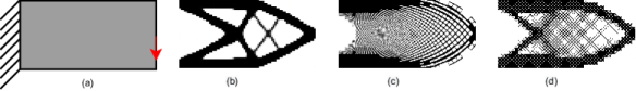
Figure 1: TO problem and solutions: (a) Mid-cantilever problem. (b) Single-scale solution. (c) Multiscale solution. (d) Graded multiscale solution using a single X-shaped microstructure.

In contrast, in multiscale topology optimization (M-TO), geometric features are computed at two or more length scales ([13],[14]). For the problem in fig. 1(a), fig. 1(c) illustrates a topology, based on a two-scale M-TO ([15]). Such designs exhibit unique characteristics such as large surface-to-volume ratio, excellent resilience, etc. This has led to a wide range of applications ([16, 17]) including energy absorption ([18]), heat exchangers ([19]), and biomedical applications ([20]). Current M-TO methods include clustering ([21, 15, 22]), kriging ([23]), multi-material ([24]), conformal lattices ([25]), etc. The advent of additive manufacturing has further spurned research in M-TO ([16]).

1.1 Graded Multiscale TO

However, one of the challenges in M-TO is the high computational cost since one must generate and evaluate various microstructures (through homogenization) during each step of the optimization process ([13, 21, 15, 26]). To reduce this cost, researchers have proposed the use of graded variations of one or more pre-selected microstructural topologies ([14, 19, 27]). [14] expressed the mechanical properties as a density function, with a B-spline-based interpolation. [19] designed graded cellular structures With triply periodic shapes. [27] parameterized the radii of each member of a lattice with linear and sinusoidal graded variations. These methods are referred to as graded multiscale TO, or GM-TO, leading to topologies such as the one illustrated in fig. 1(d), where, as an example, graded variations of a single X-shaped microstructure are used everywhere. This leads to a significant reduction in computational cost ([28]) since homogenization is not needed within the optimization loop. However, restricting the design to a single microstructure can significantly reduce performance ([29]). To further improve the performance of GM-TO, without substantially increasing the computational cost, one can use a finite number of graded microstructures.

Density-based methods: Theoretically, using a finite number of microstructures in GM-TO is analogous to using multiple materials in TO. Therefore, various authors ([30, 31, 32, 33]) proposed the use of uniform multi-phase materials interpolation (UMMI) models for GM-TO. Given the elasticity matrix of each microstructure at a particular volume fraction, two different UMMI models have been proposed for interpolation [34, 35]. The first type (UMMI-1) proposed by [31, 33], simply adds the contributions from each microstructure, and does not penalize microstructure mixing. The UMMI of the second type (UMMI-2) penalizes microstructure mixing at the cost of non-linearity ([30]). To mitigate the effect of non-linearity, [36] suggested a gradual increase in the penalty in multi-materials, further explored as a multi-scale formulation by [37, 38]. Despite penalization, microstructure mixing is not entirely eliminated in UMMI-2. Further, while multiple materials can often co-exist at a given point, this is unacceptable in GM-TO. Finally, a handful (typically less than five) materials can be sufficient in multi-material TO, while a large number of microstructures are required in GM-TO.

Level-set methods: Level-set methods are also a popular choice for GM-TO. [39, 40] considered a level-set based method where the microstructural shape is represented and parametrized by implicit functions thereby circumventing the need for homogenization within every loop; instead one can rely on curve-fitting. [41] utilized the level set function to evolve on topologies on both the micro and macroscale, with connectivity ensured by the higher-order continuity of the level-set function. [42] addressed the challenge of connectivity of microstructures through shape metamorphosis to build graded transition zones using a connectivity index. Finally, GM-TO with graded variations of a single microstructure was implemented by [43] based on the parametrized level-set functions using radial basis functions.

Data-driven methods: Recently, data-driven techniques have been proposed to address GM-TO. For instance, [44, 45] utilize a latent variable Gaussian process that embeds discrete microstructures in a continuous and differentiable latent space. While the latent space is trained on the discrete homogenized data, the procedure of snapping and re-optimization may lead to sub-optimal results. Several authors ([46, 47, 48]) replaced the expensive homogenization process with neural networks that map the design variables to the homogenized elasticity matrix. [33] used neural networks to interpolate the stiffness matrices from homogenized data. [49] used two neural networks trained on topology optimized data: one for determining the microstructural topology and the other to improve the connectivity of microstructures. One of the challenges in data-driven methods is the computational expense in data generation and training of the machine learning models. Another challenge with the data-driven methods is that physical bounds on the elasticity matrices (such as positive-definiteness) cannot be enforced explicitly, which can lead to spurious stiffness matrices and non-convergence.

1.2 Paper Contributions

In this paper, we exploit the unique classification capability of neural networks to address some of the limitations of current GM-TO methods. Specifically, we propose a graded multiscale topology optimization using neural-networks (GM-TOuNN) (section 2) framework. GM-TOuNN extends the mesh-independent neural-network (NN) based representation of the macro-scale topology proposed by [50] to GM-TO. The mesh-independent representation allows us to consider a large number of candidate microstructures without increasing the number of design variables. Further, the partition of unity is implicitly guaranteed by the NN construction. Finally, one can leverage automatic differentiation (AD) of the NN computational framework to provide end-to-end differentiability and automated sensitivity analysis. Numerical experiments are presented in section 3. We conclude with limitations and future work in section 4.

2 Proposed Method

2.1 Problem Specification

Consider a design domain with prescribed loads, restraints and a set of microstructural topologies (fig. 2). In the current work, we seek to compute an optimal multiscale design where we determine, at every location, the appropriate microstructure and its size-parameter (gradation). For simplicity, we will assume the compliance must be minimized subject to a volume constraint.

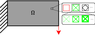
Figure 2: A GM-TO problem.

To assist in optimization, we introduce the following design variables. The presence or absence of a microstructure $m$ at any point $\bm{x}$ will be denoted by the variable $\rho_{m}(\bm{x})$, where, ideally, $\rho_{m}(\bm{x})\in\{0,1\}$. However, for continuous gradient-based optimization, we will let $0\leq\rho_{m}\leq 1$ and drive it towards $0/1$ through penalization. Thus, at any point $\bm{x}$, one can define the vector $\bm{\rho}(\bm{x})=\{\rho_{1}(\bm{x}),\rho_{2}(\bm{x}),\ldots,\rho_{M}(\bm{x})\}$ that captures the presence or absence of the $M$ microstructures with the partition of unity constraint $\sum\rho_{m}(\bm{x})=1$. Further, since the microstructures are graded, we control their size by the scalar design variable $0\leq v(\bm{x})\leq 1$ where 0 denotes a void and 1 denotes a complete fill. Thus, in conclusion, $\bm{\rho}(\bm{x})$ dictates the type of microstructure, while $v(\bm{x})$ dictates the size or volume fraction of the microstructure at $\bm{x}$.

Consequently, one can pose the GM-TO problem in a discrete finite-element setting as:

$$\underset{\bm{\rho},\bm{v}}{\text{minimize}} J(\bm{\rho},\bm{v})=\bm{f}^{T}\bm{u}$$ (1a)

subject to $$\bm{K}(\bm{\rho},\bm{v})\bm{u}=\bm{f}$$ (1b)

$$g_{v}(\bm{v})\coloneqq\frac{\sum\limits_{e}v(\bm{x}_{e})A_{e}}{V_{f}^{*}\sum\limits_{e}A_{e}}-1\leq 0$$ (1c)

$$\sum\limits_{m=1}^{M}\rho_{m}(\bm{x})=1\;,\;\forall\bm{x}$$ (1d)

$$0\leq\rho_{m}(\bm{x})\leq 1\;,\;\forall\bm{x}\;,\;\forall m$$ (1e)

$$0\leq v(\bm{x})\leq 1\;,\;\forall\bm{x}$$ (1f)

where $J$ is the structural compliance, $\bm{K}$ is the finite element stiffness matrix, $\bm{u}$ is the displacement field, $\bm{f}$ is the applied force, $V_{f}^{*}$ the maximum allowed volume fraction, with $A_{e}$ is the area (2D) of the element $e$.

2.2 Design Representation using Neural Networks

Typically, for such problems, the design variables are captured via the underlying FE mesh ([51]), i.e., for the above problem, design variables $\bm{\rho}_{e}$ and $v_{e}$ are defined at each element $e$. Thus the number of design variables grows linearly with the mesh size. Further, observe that the partition of unity constraint must be imposed over each element.

In this paper, we avoid this undesirable growth in complexity by indirectly controlling the design variables via a coordinate-based neural-network ([50, 52]). The proposed neural-network (NN) architecture (see fig. 3) consists of the following entities:

1. Input Layer: The input to the NN are points $\bm{x}\in\mathbf{R}^{d}$ ($d=2$ for 2D) within the domain.

2. Hidden Layers: The hidden layers consists of a series of Swish ($x.sigmoid(x)$, [53]) activated dense layers.

3. Output Layer: The output layer consists of $M+1$ neurons corresponding to the microstructure composition $\bm{\rho}=\{\rho_{1},\rho_{2},\ldots\rho_{M}\}$ and the volume fraction $v$. Further, the neurons associated with $\bm{\rho}$ are activated by a softmax function. This guarantees that the partition of unity ($\sum\rho_{i}=1$) and physical validity $0\leq\rho_{i}\leq 1$ are automatically satisfied. The output neuron associated with volume fraction is activated via a Sigmoid function, ensuring that $0\leq v(\bm{x})\leq 1$. Thus, no additional constraint are needed.

4. Design Variables: The weights and bias, denoted by the $\bm{w}$, now become the primary design variables, i.e., we have $\bm{\rho}(x,y;\bm{w})$ and $v(x,y;\bm{w})$.

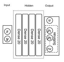
Figure 3: Neural network architecture used for GM-TOuNN.

Thus the strategy is to perform GM-TO via the NN weights $\bm{w}$, i.e., the GM-TO problem in eq. 1 reduces to:

$$\underset{\bm{w}}{\text{minimize}} J(\bm{w})=\bm{f}^{T}\bm{u}(\bm{w})$$ (2a)

subject to $$\bm{K}(\bm{w})\bm{u}=\bm{f}$$ (2b)

$$g_{v}(\bm{w})\coloneqq\frac{\sum\limits_{e}v(\bm{x}_{e};\bm{w})A_{e}}{V_{f}^{*}\sum\limits_{e}A_{e}}-1\leq 0$$ (2c)

Observe that: (1) no additional constraint is needed since they are automatically satisfied by the NN, and (2) increasing the number of candidate microstructures only increases the number of output neurons but not the number of design variables.

2.3 Material Model

Given the NN-architecture, one can now proceed to construct the material model for analysis. Towards this end, let $[C_{m}(v)]$ be the elasticity matrix of microstructure $m$ at volume fraction $v$, where $[C_{m}(v)]$ consists of six independent components (in 2D):

$$[C_{m}(v)]=\begin{bmatrix}C_{11}(v)&C_{12}(v)&C_{13}(v)\\ &C_{22}(v)&C_{23}(v)\\ \lx@intercol\hfil\text{sym.}\hfil\lx@intercol&C_{33}(v)\end{bmatrix}$$ (3)

To obtain $[C_{m}(v)]$, we adopt a simple constrained polynomial scheme ([54]). Specifically, the homogenized constitutive matrix [55] for microstructure $m$ is evaluated at a few instances of volume fractions. Then, a polynomial ensuring positive definiteness is interpolated to these instances for each of the components. As an example, the polynomials for an X-type microstructure are illustrated in fig. 4.

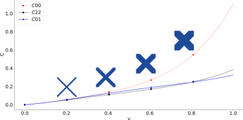
Figure 4: Polynomial fit of the components of constitutive matrix for the $X$ type microstructure (note: $C_{00}=C_{11}$)

Given $[C_{m}(v)]$ for each microstructure $m$, the effective elasticity matrix at any location $\bm{x}$ is defined here as a weighted average ([34]):

$$[C(\bm{\rho},v)]=\sum\limits_{m=1}^{M}\rho_{m}^{p}[C_{m}(v)]$$ (4)

where $p$ is the solid isotropic material with penalization (SIMP) constant. The penalization discourages intermediate volume fractions, i.e., discourages microstructure mixing.

2.4 Finite Element Analysis

We will use conventional finite element analysis (FEA) as part of the framework. Here, we use a structured quadrilateral mesh due to its simplicity. The element stiffness matrix is defined as:

$$[K_{e}]=\int\limits_{\Omega_{e}}[\nabla N_{e}]^{T}[C(\bm{x}_{e})][\nabla N_{e}]d\Omega_{e}$$ (5)

where $[\nabla N_{e}]$ is the gradient of the shape matrix, and $[C(\bm{x}_{e})]$ is the elasticity tensor evaluated at the center of the element.

In a straightforward, but naïve, implementation, one would evaluate $\bm{\rho}$ and $v$ at the center of each element via the NN. Then, given the pre-computed polynomials $[C_{m}(v)]$, one would then find the effective $[C]$ for that element via eq. 4. Finally the element stiffness matrices will be computed via eq. 5. Thus the element stiffness matrices must be computed for each element, and for each step of the optimization process. This can be computationally very expensive. To significantly reduce the computation, we exploit the concept of template stiffness matrices proposed by [15].

Observe that one can express the element stiffness matrix as follows:

$$=C_{11}[\hat{K}^{1}]+C_{22}[\hat{K}^{2}]+C_{33}[\hat{K}^{3}]$$ (6)

$$+C_{12}[\hat{K}^{4}]+C_{13}[\hat{K}^{5}]+C_{23}[\hat{K}^{6}]$$

where,

$$[\hat{K}^{i}]=\int\limits_{\Omega_{e}}[\nabla N_{e}]^{T}[\hat{C}^{i}][\nabla N_{e}]d\Omega_{e},\quad i=1,2,\ldots 6$$ (7)

and

$$[\hat{C}^{1}]=\begin{bmatrix}1&0&0\\ 0&0&0\\ 0&0&0\\ \end{bmatrix}\;[\hat{C}^{2}]=\begin{bmatrix}0&0&0\\ 0&1&0\\ 0&0&0\\ \end{bmatrix}\quad\;[\hat{C}^{3}]=\begin{bmatrix}0&0&0\\ 0&0&0\\ 0&0&1\\ \end{bmatrix}$$

$$[\hat{C}^{4}]=\begin{bmatrix}0&1&0\\ 1&0&0\\ 0&0&0\\ \end{bmatrix}\;[\hat{C}^{5}]=\begin{bmatrix}0&0&1\\ 0&0&0\\ 1&0&0\\ \end{bmatrix}\quad\;[\hat{C}^{6}]=\begin{bmatrix}0&0&0\\ 0&0&1\\ 0&1&0\\ \end{bmatrix}$$ (8)

Thus the matrices $[\hat{K}^{i}]$ are computed at the start of the optimization. Then, during optimization, the element stiffness matrices are computed efficiently via eq. 6. In other words, one would evaluate $\bm{\rho}$ and $v$ at the center of each element via the NN. Then, given the pre-computed polynomials $[C_{m}(v)]$, one would then find the effective $[C]$ for that element (as before). But, to compute the element stiffness matrices, we will rely on eq. 6 This will be followed by the assembly of the global stiffness matrix $\bm{K}$.

2.5 Loss Function

We now consider solving the NN-based optimization problem in eq. 2. Neural networks are designed to minimize a loss function using well-known optimization techniques such as Adam procedure ([56]). We therefore convert the constrained minimization problem into a loss function minimization by employing a log-barrier scheme as proposed in [57]. Specifically, the loss function is defined as

$$L(\bm{w})=J+\psi(g_{v})$$ (9)

where,

$$\psi_{t}(g)=\begin{cases}-\frac{1}{t}\log(-g)\;,\quad g\leq\frac{-1}{t^{2}}\\ tg-\frac{1}{t}\log(\frac{1}{t^{2}})+\frac{1}{t}\;,\quad\text{otherwise}\end{cases}$$ (10)

where the parameter $t$ is updated during each iteration, making the enforcement of the constraint stricter as the optimization progresses.

2.6 Sensitivity Analysis

Since Adam is a gradient-based optimizer, it requires sensitivities, i.e., derivative of the loss function (eq. 9) with respect to the design variable (weights of the NN $\bm{w}$). Fortunately, one can exploit modern automatic differentiation frameworks ( [58]) to avoid manual sensitivity calculations. In particular, expressing all our computation, including FEA within JAX ([59]), results in an end-to-end differentiable framework, as illustrated in fig. 5.

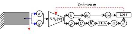
Figure 5: Optimization loop of the proposed GM-TOuNN framework.

2.7 Algorithm

We summarize the proposed framework in algorithm 1. We will assume that a GM-TO problem, a desired volume fraction, an NN configuration and a set of microstructures with their interpolated coefficients are given.

The first step in the algorithm is to discretize the domain with a finite element mesh, and sample the mesh (3) at the center of each element (these serve as inputs to the NN). We compute the template stiffness matrices (4). The log barrier penalty $t$ and SIMP penalty parameter are also initialized (5).

In the main iteration, the element volume fraction $v$ and microstructure field $\bm{\rho}$ are computed using the NN using the current values of $\bm{w}$ (7). These fields are then used to construct the stiffness matrix and to solve for the displacement (8 - 12). Then we compute the objective (13) and volume constraint (14), leading to the loss function (15). The weights $\bm{w}$ are then updated using the Adam optimization scheme (17). The optimizer requests the sensitivities which are computed in an automated fashion (16). Finally the log-barrier penalty and SIMP penalty parameters are updated (19 and 20). The process is repeated until termination, i.e., till the relative change in loss is below a certain threshold or the iterations exceed a maximum value. Upon termination, each element is replaced with an image of the associated microstructure with the desired volume fraction. The framework is schematically depicted in fig. 5.

Algorithm 1 Graded Mutliscale TO

1:procedure GMTOuNN($\Omega_{0}$, BC, $V_{f}^{*}$, …) $\triangleright$ Inputs

2:     $\Omega^{0}\rightarrow\Omega^{0}_{h}$ $\triangleright$ Discretize domain for FE

3:     $\bm{x}=\{x_{e},y_{e}\}_{e\in\Omega^{0}_{h}}$ $\triangleright$ elem centers; NN input

4:     $\Omega^{0}_{h}\rightarrow[\hat{K}]$ $\triangleright$ Compute stiff. templates eq. 7

5:     k = 0; $t=t_{0}$; $p=1$ $\triangleright$ Initialization

6:     repeat$\triangleright$ Optimization (Training)

7:         $NN(\bm{x}_{e};\bm{w})\rightarrow\{\bm{\rho},v\}_{e}$ $\triangleright$ Fwd prop NN

8:         $v\rightarrow[C_{m}]\;m=1,\ldots,M\;\forall e$$\triangleright$ elasticity matr. eq. 3

9:         $\{[C_{m}],\rho_{m}\}_{e}\rightarrow[C]_{e}$ $\triangleright$ net elasticity matrix eq. 4

10:         $\{[C],[\hat{K}]\}_{\forall e}\rightarrow[K]_{e}$ $\triangleright$ elem stiff matrices eq. 6

11:         $\bigcup\limits_{e}[K]_{e}\rightarrow[K]$ $\triangleright$ global stiff matrix

12:         $\{[K],\bm{f}\}\rightarrow\bm{u}$ $\triangleright$ FEA eq. 2b

13:         $\{\bm{f},\bm{u}\}\rightarrow J$ $\triangleright$ Objective, Equation 2a

14:         $\{v_{e},V_{f}^{*}\}\rightarrow g_{v}$ $\triangleright$ vol cons, eq. 2c

15:         $\{J,g_{v}\}\rightarrow L$ $\triangleright$ Loss from Equation 9

16:         $AD(L\leftarrow\bm{w})\rightarrow\nabla L$ $\triangleright$ sensitivity analysis

17:         $w+\Delta w(\nabla L)\rightarrow w$ $\triangleright$ Adam optimizer [56] step

18:         $\text{k}++$

19:         $t=t_{0}\mu^{k}$ $\triangleright$ Increment $t$; log-barrier term

20:         $p=p+\Delta p$ $\triangleright$ SIMP penalty update

21:     until  $||\Delta L||<\epsilon^{*}$ and $k<k_{max}$ $\triangleright$ convg. criteria

22:     return $\bm{w},\bm{\rho},\bm{v}$

23:end procedure

3 Numerical examples

In this section, we conduct several experiments to illustrate the method and algorithm. The default settings are as follows:

• Mesh: A mesh size of $60\times 30$ with elements of size $1\times 1$ is used for all experiments, unless otherwise stated; the force is assumed to be 1 unit.

• Material: The microstructures are assumed to be composed of an isotropic material with a Poisson’s ratio $\nu=0.3$ and Young’s modulus $E=1$.

• Neural Network: The NN comprises of 4 Swish-activated hidden layers with 20 neurons in each layer.

• Candidate Microstructures: A set of 11 predefined microstructures (fig. 6) are used in the experiments. Observe that connectivity between these microstructures is guaranteed. A quintic polynomial is used to interpolate the components of the constitutive matrix.

• Material Penalization: The SIMP penalization constant $p$ in eq. 4 is incremented every iteration by $0.02$ using the continuation scheme [60], starting from a value of $1$, capped at $8$.

• Loss Function: The constraint penalty values of $t_{0}=1$ and $\mu=1.01$ is used.

• Optimizer: Adam optimizer with a learning rate of $0.01$ is used. Further, the gradients are clipped at a maximum norm of 1 to improve stability of convergence ([61]). A maximum of 300 iterations were allowed with $\epsilon^{*}=0.01$

• Computing Environment: All experiments are conducted on a MacBook M1 Pro, using the JAX ([59]) environment.

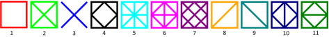
Figure 6: Microstructures considered in the experiments.

3.1 Validation

Consider the simple tensile bar problem in fig. 7(a). Although eleven microstructures were provided (see fig. 6), the final topology in fig. 7(b) consists of a single microtopology (number 1) with a complete fill for all elements in the middle and void at the top and bottom, i.e., the result is consistent with expectations. The optimization converged in 240 iterations, taking 47 seconds.

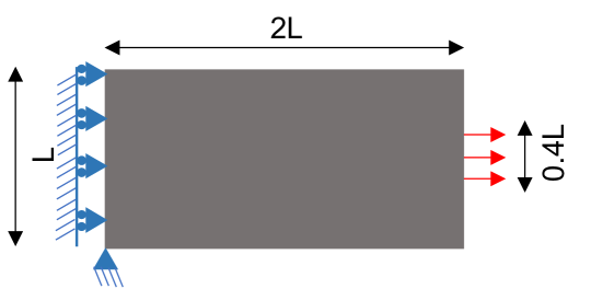
(a) Loading of a tensile bar.

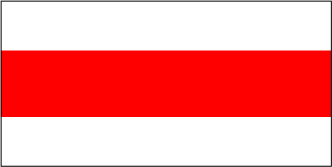
(b) GM-TO of a tensile bar with $V_{f}^{*}=0.4$ ($J^{*}=183$).

Figure 7: A tensile-bar problem.

Next, we consider an MBB beam in fig. 8(a). [54] reported compliance values between $76$ and $88$ when considering only one microstructure at a time. In comparison, we achieve a compliance of $68$ when all microstructures are allowed; see fig. 8(b).

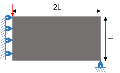
(a) Loading of an MBB beam.

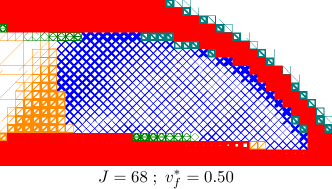
(b) Optimized MBB beam.

Figure 8: GM-TO of an MBB beam.

Next, we consider an L-bracket (800 elements) illustrated in fig. 9. Using only a single X-type microstructure, [54] achieved a compliance of 1130, 283, 171 for volume fractions of 0.1, 0.3 and 0.5 respectively. By considering all microstructures (fig. 10), we achieved compliance of 1048, 263 and 158 respectively.

Figure 9: Loading of an L-bracket

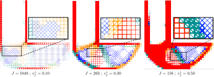
Figure 10: GM-TO of an L-bracket at various volume fractions.

Finally, we consider an edge-loaded beam with a mesh of $32\times 20$ elements illustrated in fig. 11(a). Here, the design is constrained to have the same microstructure along the X-axis (but can vary along the Y-Axis), with a desired volume fraction $V_{f}^{*}=0.6$. The topology and compliance obtained (fig. 11(c)) is validated against the one reported by [15] (fig. 11(b)).

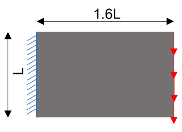
(a) Edge-loaded beam.

(b) M-TO design ($J=1.45e5$) obtained by [15].

(c) GM-TO design ($J=1.41e5$) obtained using the proposed method.

Figure 11: Validation for an edge-loaded beam.

3.2 Convergence Study

We illustrate the typical convergence of the proposed algorithm for a mid-cantilever beam (fig. 1(a)) for $V_{f}^{*}=0.5$. The compliance, volume fraction and the evolving topology at various instances are illustrated in fig. 12. We observe that the log-barrier formulation leads to a stable convergence. Similar convergence behavior was observed for all other examples. The computation took $53$ secs.

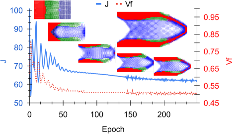
Figure 12: Convergence of compliance and volume fraction for a mid-cantilever beam. Topologies are illustrated at the $0^{\text{th}}$, $50^{\text{th}}$, $100^{\text{th}}$, $150^{\text{th}}$, $200^{\text{th}}$ and $250^{\text{th}}$(final) iterations.

3.3 Varying number of microstructures

Two central hypotheses of the current work is that one can achieve better designs with larger number of candidate microstructures, and the framework is (computationally) insensitive to the number of candidates. To validate these, consider the problem in fig. 8(a). The topologies and compliance values when allowing for varying number of microstructures, in the order in which they are present in fig. 6, are illustrated in fig. 13, As expected, the compliance improves as we allow for larger number of microstructures. As noted earlier, each additional candidate microstructure requires only one additional output neuron (2 additional design variables), enabling us to consider large set of microstructures if necessary. The computational time was approximately $56$ seconds, independent of the number of microstructures.

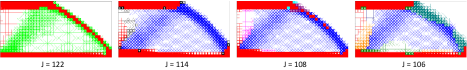
Figure 13: Design and compliance using 2, 4, 7 and 11 microstructures.

3.4 Pareto Designs

Exploring the Pareto-front is critical in making design choices and understanding the trade-off between the objective and constraint. Consider once again the mid-cantilever beam in fig. 1(a). We illustrate the compliance values and topologies for varying volume fractions $V_{f}^{*}$ in fig. 14.

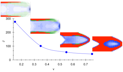
Figure 14: Pareto designs of mid-cantilever beam.

3.5 Mesh and NN Dependency

Next we study the effect of NN size and FE mesh on the computed topology using the tip cantilever (fig. 2) as an example; all other parameters are kept constant. For varying NN size, the topologies are reported in fig. 15; no appreciable difference in computational time was observed. Similarly, fig. 16 captures the topologies for varying mesh size; the computational times were 7.5, 24.7 and 114.3 seconds per 100 iterations for the $40\times 20$, $60\times 30$ and $80\times 40$ mesh respectively.

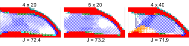
Figure 15: GM-TO of a tip cantilever at $V_{f}^{*}=0.45$ with varying NN size.

Figure 16: GM-TO of a tip cantilever at $V_{f}^{*}=0.25$ with varying mesh size.

3.6 High Resolution Design

In the proposed method, one can perform optimization on a coarse mesh and then re-sample at a higher resolution to populate the microstructures, resulting in smoother variation in the microstructure topologies. Note that, even after re-sampling, the framework guarantees partition of unity. However, due to NN-interpolation, microstructure mixing can occur on the finer mesh at the interfaces. This was resolved by choosing the microstructure $m$ with the largest $\rho_{m}$. This is illustrated in fig. 17 where we optimize on a $40\times 20$ mesh and then re-sample on a $80\times 40$ mesh.

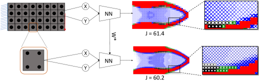
Figure 17: Extraction of high resolution design with smoother variation of microstructures.

4 Conclusions

A framework for graded multi-scale topology optimization using neural network was proposed and demonstrated. The salient features of this framework are: (1) the number of design variables are only weakly dependent on the number of pre-selected microstructures, (2) the partition of unity constraint is automatically satisfied, and (3) manual sensitivity calculations is avoided.

The framework was limited to 2D compliance minimization problems, involving microstructures governed by a single size parameter. Extension to 3D, non-compliance problems (such as energy absorption [62], orthopedic implants [63], resonant frequencies [64]) using more generic multi-parameter microstructures need to be explored. Furthermore, while we relied on polynomials for directly interpolating the elasticity components, it is desirable to consider an Eigen-value decomposition ([54]) for increased robustness. The framework can complement and might benefit from data driven approaches ([44, 45]). Finally, while we relied on the simple Adam optimization procedure, second order optimization methods such as LBFGS might result in better/faster convergence ([65]).

Replication of Results

The Python code pertinent to this paper is available at github.com/UW-ERSL/GMTOuNN

Compliance with ethical standards

The authors declare that they have no conflict of interest.

References

- [1] M. P. Bendsøe and O. Sigmund. Topology optimization. Springer Berlin Heidelberg, 2004.
- [2] O. Sigmund and K. Maute. Topology optimization approaches: A comparative review. Structural and Multidisciplinary Optimization, 48(6):1031–1055, 2013.
- [3] M. P. Bendsøe. Optimal shape design as a material distribution problem. Structural Optimization, 1(4):193–202, 1989.
- [4] M. P. Bendsøe and N. Kikuchi. Generating optimal topologies in structural design using a homogenization method. Computer Methods in Applied Mechanics and Engineering, 71(2):197–224, nov 1988.
- [5] B. Hassani and E. Hinton. A review of homogenization and topology optimization I - Homogenization theory for media with periodic structure. Computers and Structures, 69(6):707–717, 1998.
- [6] J. A. Sethian and Andreas Wiegmann. Structural Boundary Design via Level Set and Immersed Interface Methods. Journal of Computational Physics, 163(2):489–528, 2000.
- [7] M.Y. Wang, X. Wang, and D. Guo. A level set method for structural topology optimization. Computer Methods in Applied Mechanics and Engineering, 192(1-2):227–246, jan 2003.
- [8] Y. M. Xie and G. P. Steven. A simple evolutionary procedure for structural optimization. Computers and Structures, 49(5):885–896, dec 1993.
- [9] X. Y. Yang, Y. M. Xei, G. P. Steven, and O. M. Querin. Bidirectional evolutionary method for stiffness optimization. AIAA Journal, 37(11):1483–1488, nov 1999.
- [10] W. Zhang, J. Yuan, J. Zhang, and X. Guo. A new topology optimization approach based on Moving Morphable Components (MMC) and the ersatz material model. Structural and Multidisciplinary Optimization, 53(6):1243–1260, 2016.
- [11] K. Suresh. A 199-line Matlab code for Pareto-optimal tracing in topology optimization. Structural and Multidisciplinary Optimization, 42(5):665–679, 2010.
- [12] Shiguang Deng and Krishnan Suresh. Multi-constrained topology optimization via the topological sensitivity. Structural and Multidisciplinary Optimization, 51(5):987–1001, 2015.
- [13] H. C. Rodrigues, J. M. Guedes, and M. P. Bendsøe. Hierarchical optimization of material and structure. Structural and Multidisciplinary Optimization, 24(1):1–10, 2002.
- [14] Y. Wang, H. Xu, and D. Pasini. Multiscale isogeometric topology optimization for lattice materials. Computer Methods in Applied Mechanics and Engineering, 316:568–585, 2017.
- [15] Tej Kumar and Krishnan Suresh. A density-and-strain-based k-clustering approach to microstructural topology optimization. Structural and Multidisciplinary Optimization, 61(4):1399–1415, 2020.
- [16] Wenjin Tao and Ming C. Leu. Design of lattice structure for additive manufacturing. In 2016 International Symposium on Flexible Automation (ISFA), pages 325–332. IEEE, aug 2016.
- [17] Y. Wang, L. Zhang, S. Daynes, H. Zhang, S. Feih, and M. Y. Wang. Design of graded lattice structure with optimized mesostructures for additive manufacturing. Materials and Design, 142:114–123, 2018.
- [18] Lin Cheng, Xuan Liang, Jiaxi Bai, Qian Chen, John Lemon, and Albert To. On utilizing topology optimization to design support structure to prevent residual stress induced build failure in laser powder bed metal additive manufacturing. Additive Manufacturing, 27(March):290–304, 2019.
- [19] Dawei Li, Ning Dai, Yunlong Tang, Guoying Dong, and Yaoyao Fiona Zhao. Design and Optimization of Graded Cellular Structures with Triply Periodic Level Surface-Based Topological Shapes. Journal of Mechanical Design, Transactions of the ASME, 141(7), 2019.
- [20] Fei Liu, Zhongfa Mao, Peng Zhang, David Z. Zhang, Junjie Jiang, and Zhibo Ma. Functionally graded porous scaffolds in multiple patterns: New design method, physical and mechanical properties. Materials & Design, 2018.
- [21] R. Sivapuram, P. D. Dunning, and H. A. Kim. Simultaneous material and structural optimization by multiscale topology optimization. Structural and Multidisciplinary Optimization, 54(5):1267–1281, 2016.
- [22] Jiao Jia, Daicong Da, Cha-Liang Loh, Haibin Zhao, Sha Yin, and Jun Xu. Multiscale topology optimization for non-uniform microstructures with hybrid cellular automata. Structural and Multidisciplinary Optimization, 62(2):757–770, 2020.
- [23] Yan Zhang, Hao Li, Mi Xiao, Liang Gao, Sheng Chu, and Jinhao Zhang. Concurrent topology optimization for cellular structures with nonuniform microstructures based on the kriging metamodel. Structural and Multidisciplinary Optimization, 59(4):1273–1299, apr 2019.
- [24] Y. Zhang, M. Xiao, H. Li, L. Gao, and S. Chu. Multiscale concurrent topology optimization for cellular structures with multiple microstructures based on ordered SIMP interpolation. Computational Materials Science, 155:74–91, dec 2018.
- [25] Tongyu Wu and Shu Li. An efficient multiscale optimization method for conformal lattice materials. Structural and Multidisciplinary Optimization, 63(3):1063–1083, 2021.
- [26] Xuechen Gu, Shaoming He, Yihao Dong, and Tao Song. An improved ordered simp approach for multiscale concurrent topology optimization with multiple microstructures. Composite Structures, 287:115363, 2022.
- [27] Dilaksan Thillaithevan, Paul Bruce, and Matthew Santer. Stress-constrained optimization using graded lattice microstructures. Structural and Multidisciplinary Optimization, 63(2):721–740, 2021.
- [28] C. Wang, J. H. Zhu, W. H. Zhang, S. Y. Li, and J. Kong. Concurrent topology optimization design of structures and non-uniform parameterized lattice microstructures. Structural and Multidisciplinary Optimization, 58(1):35–50, 2018.
- [29] Zijun Wu, Fei Fan, Renbin Xiao, and Lianqing Yu. The substructuring‐based topology optimization for maximizing the first eigenvalue of hierarchical lattice structure. International Journal for Numerical Methods in Engineering, page nme.6342, mar 2020.
- [30] Zhen Liu, Liang Xia, Qi Xia, and Tielin Shi. Data-driven design approach to hierarchical hybrid structures with multiple lattice configurations. Structural and Multidisciplinary Optimization, 61(6):2227–2235, feb 2020.
- [31] Liang Xu and Gengdong Cheng. Two-scale concurrent topology optimization with multiple micro materials based on principal stress direction. In World Congress of Structural and Multidisciplinary Optimisation, pages 1726–1737. Springer, 2017.
- [32] Yaguang Wang and Zhan Kang. Concurrent two-scale topological design of multiple unit cells and structure using combined velocity field level set and density model. Computer methods in applied mechanics and engineering, 347:340–364, 2019.
- [33] Han Zhou, Jihong Zhu, Chuang Wang, Yifei Zhang, Jiaqi Wang, and Weihong Zhang. Hierarchical structure optimization with parameterized lattice and multiscale finite element method. Structural and Multidisciplinary Optimization, 65(1):1–20, 2022.
- [34] J. Stegmann and E. Lund. Discrete material optimization of general composite shell structures. International Journal for Numerical Methods in Engineering, 62(14):2009–2027, apr 2005.
- [35] Tong Gao and Weihong Zhang. A mass constraint formulation for structural topology optimization with multiphase materials. International Journal for Numerical Methods in Engineering, 88(8):774–796, nov 2011.
- [36] Emily D. Sanders, Miguel A. Aguiló, and Glaucio H. Paulino. Multi-material continuum topology optimization with arbitrary volume and mass constraints. Computer Methods in Applied Mechanics and Engineering, 340:798–823, oct 2018.
- [37] ED Sanders, A Pereira, and GH Paulino. Optimal and continuous multilattice embedding. Science Advances, 7(16):eabf4838, 2021.
- [38] Fernando V Senhora, Emily D Sanders, and Glaucio H Paulino. Optimally-tailored spinodal architected materials for multiscale design and manufacturing. Advanced Materials, page 2109304, 2022.
- [39] Cong Hong Phong Nguyen and Young Choi. Multiscale design of functionally graded cellular structures for additive manufacturing using level-set descriptions. Structural and Multidisciplinary Optimization, 64(4):1983–1995, 2021.
- [40] Ruijie Zhao, Junpeng Zhao, and Chunjie Wang. Stress-constrained multiscale topology optimization with connectable graded microstructures using the worst-case analysis. International Journal for Numerical Methods in Engineering, 123(8):1882–1906, 2022.
- [41] Chen Yu, Qifu Wang, Zhaohui Xia, Yingjun Wang, Chao Mei, and Yunhua Liu. Multiscale topology optimization for graded cellular structures based on level set surface cutting. Structural and Multidisciplinary Optimization, 65(1):1–17, 2022.
- [42] Xiao-Yi Zhou, Zongliang Du, and H Alicia Kim. A level set shape metamorphosis with mechanical constraints for geometrically graded microstructures. Structural and Multidisciplinary Optimization, 60(1):1–16, 2019.
- [43] Hui Liu, Hongming Zong, Ye Tian, Qingping Ma, and Michael Yu Wang. A novel subdomain level set method for structural topology optimization and its application in graded cellular structure design. Structural and Multidisciplinary Optimization, 60(6):2221–2247, 2019.
- [44] Liwei Wang, Siyu Tao, Ping Zhu, and Wei Chen. Data-driven topology optimization with multiclass microstructures using latent variable gaussian process. Journal of Mechanical Design, 143(3), 2021.
- [45] Liwei Wang, Anton van Beek, Daicong Da, Yu-Chin Chan, Ping Zhu, and Wei Chen. Data-driven multiscale design of cellular composites with multiclass microstructures for natural frequency maximization. Composite Structures, 280:114949, 2022.
- [46] Li Zheng, Siddhant Kumar, and Dennis M Kochmann. Data-driven topology optimization of spinodoid metamaterials with seamlessly tunable anisotropy. Computer Methods in Applied Mechanics and Engineering, 383:113894, 2021.
- [47] Seth Watts, William Arrighi, Jun Kudo, Daniel A. Tortorelli, and Daniel A. White. Simple, accurate surrogate models of the elastic response of three-dimensional open truss micro-architectures with applications to multiscale topology design. Structural and Multidisciplinary Optimization, nov 2019.
- [48] Daniel A. White, William J. Arrighi, Jun Kudo, and Seth E. Watts. Multiscale topology optimization using neural network surrogate models. Computer Methods in Applied Mechanics and Engineering, 346:1118–1135, apr 2019.
- [49] Darshil Patel, Dustin Bielecki, Rahul Rai, and Gary Dargush. Improving connectivity and accelerating multiscale topology optimization using deep neural network techniques. Structural and Multidisciplinary Optimization, 65(4):1–19, 2022.
- [50] Aaditya Chandrasekhar and Krishnan Suresh. Tounn: topology optimization using neural networks. Structural and Multidisciplinary Optimization, 63(3):1135–1149, 2021.
- [51] Emily D. Sanders, Miguel A. Aguiló, and Glaucio H. Paulino. Multi-material continuum topology optimization with arbitrary volume and mass constraints. Computer Methods in Applied Mechanics and Engineering, 340:798–823, oct 2018.
- [52] Aaditya Chandrasekhar and Krishnan Suresh. Multi-material topology optimization using neural networks. Computer-Aided Design, 136:103017, 2021.
- [53] Prajit Ramachandran, Barret Zoph, and Quoc V Le. Searching for activation functions. arXiv preprint arXiv:1710.05941, 2017.
- [54] Tej Kumar, Saketh Sridhara, Bhagyashree Prabhune, and Krishnan Suresh. Spectral decomposition for graded multi-scale topology optimization. Computer Methods in Applied Mechanics and Engineering, 377:113670, 2021.
- [55] Erik Andreassen and Casper Schousboe Andreasen. How to determine composite material properties using numerical homogenization. Computational Materials Science, 83:488–495, 2014.
- [56] Diederik P. Kingma and Jimmy Lei Ba. Adam: A method for stochastic optimization. In 3rd International Conference on Learning Representations, ICLR 2015 - Conference Track Proceedings. International Conference on Learning Representations, ICLR, dec 2015.
- [57] Hoel Kervadec, Jose Dolz, Jing Yuan, Christian Desrosiers, Eric Granger, and I Ben Ayed. Constrained deep networks: Lagrangian optimization via log-barrier extensions. CoRR, abs/1904.04205, 2(3):4, 2019.
- [58] Aaditya Chandrasekhar, Saketh Sridhara, and Krishnan Suresh. Auto: a framework for automatic differentiation in topology optimization. Structural and Multidisciplinary Optimization, 64(6):4355–4365, 2021.
- [59] James Bradbury, Roy Frostig, Peter Hawkins, Matthew James Johnson, Chris Leary, Dougal Maclaurin, George Necula, Adam Paszke, Jake VanderPlas, Skye Wanderman-Milne, and Qiao Zhang. JAX: composable transformations of Python+NumPy programs, 2018.
- [60] O. Sigmund and J. Petersson. Numerical instabilities in topology optimization: A survey on procedures dealing with checkerboards, mesh-dependencies and local minima. Structural Optimization, 16(1):68–75, 1998.
- [61] Razvan Pascanu, Tomas Mikolov, and Yoshua Bengio. Understanding the exploding gradient problem. CoRR, abs/1211.5063, 2012.
- [62] Wen Zhang, TX Yu, and Jun Xu. Uncover the underlying mechanisms of topology and structural hierarchy in energy absorption performances of bamboo-inspired tubular honeycomb. Extreme Mechanics Letters, 52:101640, 2022.
- [63] Nicola Ferro, Simona Perotto, Daniele Bianchi, Raffaele Ferrante, and Marco Mannisi. Design of cellular materials for multiscale topology optimization: application to patient-specific orthopedic devices. Structural and Multidisciplinary Optimization, 65(3):1–26, 2022.
- [64] Morgan Nightingale, Robert Hewson, and Matthew Santer. Multiscale optimisation of resonant frequencies for lattice-based additive manufactured structures. Structural and Multidisciplinary Optimization, 63(3):1187–1201, 2021.
- [65] Jorge Nocedal and Stephen Wright. Numerical optimization. Springer Science & Business Media, 2006.