DRAGON (Differentiable Graph Execution) : A suite of Hardware Simulation and Optimization tools for Modern Workloads

Abstract

We introduce DRAGON, an open-source, fast and explainable hardware simulation and optimization toolchain that enables hardware architects to simulate hardware designs, and to optimize hardware designs to efficiently execute workloads.

The DRAGON toolchain provides the following tools: Hardware Model Generator (DGen), Hardware Simulator (DSim) and Hardware Optimizer (DOpt).

DSim provides the simulation of running algorithms (represented as data-flow graphs) on hardware described. DGen describes the hardware in detail, with user input architectures/technology (represented in a custom description language). A novel methodology of gradient descent from the simulation allows us optimize the hardware model (giving the directions for improvements in technology parameters and design parameters), provided by Dopt.

DRAGON framework (DSim) is much faster than previously avaible works for simulation, which is possible through performance-first code writing practices, mathematical formulas for common computing operations to avoid cycle-accurate simulation steps, efficient algorithms for mapping, and data-structure representations for hardware state.

DRAGON framework (Dopt) generates performance optimized architectures for both AI and Non-AI Workloads, and provides technology targets for improving these hardware designs to 100x-1000x better computing systems.

1 Introduction

21st-century computing systems are dramatically different from the 20th-century ones. Unlike traditional processors that dominated 20th-century computing, domain-specific accelerators are rising in the 21st century. The diversity of applications, algorithms and accelerator hardware architectures is changing very rapidly. For example, more than 200 hardware accelerators for AI inference and training have been published over the past 3-4 years. Beyond AI, hardware accelerators for data analytics, graph processing, genomics and security are also growing.

In addition, the computing demands of many of these applications are increasing at unprecedented rates. For example, the computing demands of AI workloads are doubling every 3-4 months. The latest GPT-3 by OpenAI requires 355 GPU-years to train.

Major opportunities created by these 21st-century computing trends also bring their unique challenges: Traditional processor simulators are no longer sufficient to create 21st century hardware architectures. Creating a different simulator for each application-accelerator configuration is infeasible.

Supporting a new algorithm and architecture using current simulators requires significant development time (many person-months). By the time simulators are created, the accelerators they target often become obsolete. To keep up with the fast pace, new simulation frameworks are required.

The performance (throughput, energy) demands of emerging applications cannot be met by architectural improvements or (incremental) technology improvements alone. While accelerators bring benefits over processors, further improvements (e.g., 100X Energy-Delay-Product (EDP) benefits) require significant technology improvements in conjunction with architecture improvements. This creates a critical need to translate application needs into technology targets.

We propose a new, elegant, fast and explainable framework (Fig. 1) for end-to-end joint co-exploration and co-optimization of technologies, architectures and algorithms. Our framework overcomes the above challenges.

The features of our framework are:

• Fast Performance Estimation (both energy and throughput) for a wide range of AI (inference and training) and non-AI workloads on many accelerator architectures.

• Technology Target derivation from workload performance objective (in terms of execution time, energy consumption etc.). It is a first of its kind feature which runs in seconds vs. traditional trial and error approaches that can be highly inaccurate (i.e., can miss important design points during technology space exploration) and slow (i.e., weeks or longer per exploration).

• Accelerator architecture design optimization for those technology targets (e.g., in terms of systolic array structure, processing element dimensions, global buffer organization, connectivity to on-chip and off-chip memory for AI accelerators and the entire compute-memory subsystem for non-AI accelerators) that achieve desired system-level performance (e.g, Energy Efficiency, Execution Time). Our framework provides accelerator design generation for a wide range of workloads, with designs supporting multiple data-flow graphs, all within a time frame of a few seconds.

Our results are made possible by our unique approach which utilizes the (1) differentiable component (memory, compute, interconnects, connectivity) models from the technology parameter space created in the background, (2) combines the created component models with workload data flow/control-data flow graphs through appropriate scheduling/mapping steps for fast performance estimation, and (3) uses special (and provably correct) techniques to derive gradients of application performance metrics with respect to technology parameters.

The paper is organized as follows : Section 2 provides our methodology which creates data-flow graph and control-data graph representation for supporting multiple types of AI workloads, and Non-AI workloads respectively. User can specify different accelerator designs in a custom Architecture-description language (ADL) for the support of multiple data-flow AI/ control data-flow Non-AI architectures. The architecture description taken as input is used to create a hardware representation and a mapping process of the data-flow/control-data flow graph on the accelerator is used to generate the performance outputs (latency, energy consumption, resource utilization).

Section 3 provides the methodology that describes a Technology Description Language, and takes device-level technology parameters as input. Section 4 describes custom functions created to utilize device-level technology parameters and design parameters from ADL to create performance models (latency/energy etc.) of hardware components. Section 5 describes utilizing hardware component performance models to generate execution statistics for the entire application.

2 Background

A number of performance estimation simulators exist in computer architecture [1, 13, 4, 5, 16, 12, 14, 15], which given an application can produce the performance estimates of its execution latency and energy consumption.

AI-specific simulators such as Scale-Sim [11], Timeloop [10], NN-Dataflow [17], Zig-Zag [9], NAAS [7], have also been created which target a subset of CNN-specific workloads, but don’t support modern AI workloads such as Transformers, Graph Neural Networks, Deep Recommendation Models, Generative Models etc.

Running large AI workloads in these simulators is still a slow process, because the development of these simulators are not designed with runtime as a first priority.

Further, these simulators cater to one or the other subset of architectures and don’t support the wide-range of architectures we support.

Table 1 compares the capabilities of our framework with other open source available tools.

Simulators	Perf. Est.	Mapping	CNNs	DLRMs/ Transformers/ GNNs	Non-AI Workloads	Algorithm Search	Derive Accel. Design	Derive Techn. Targets.	Run Time (Avg.)
Scale-Sim (ARM) [11]	Latency	Single	✓	✗	✗	✗	✗	✗	$\sim 10^{3}$
Timeloop (Nvidia)	Latency, Energy	Single	✓	✗	✗	✗	✗	✗	$\sim 10^{2}$
NN-Dataflow [17]	Latency	Multiple (for maximal reuse)	✓	✗	✗	✗	✗	✗	$\sim 5*10^{2}$
Zig-Zag [9]	Latency, Energy	Multiple	✓	✗	✗	✗	Yes, (Memory Design using Sweep)	✗	$\sim 10^{4}$
NAAS[7]	Latency, Energy	Multiple	✓	✗	✗	✓	✓	✗	–
Ours	Latency, Energy	Multiple (w.r.t objective)	✓	✓	✓	✓	Yes, Single-Pass	Yes, Single-Pass	1

Table 1: Comparison of our Work with Previously Published Results

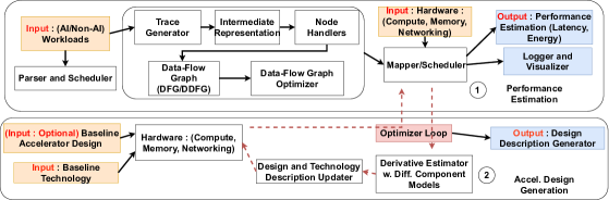
Figure 1: Overview of the Framework

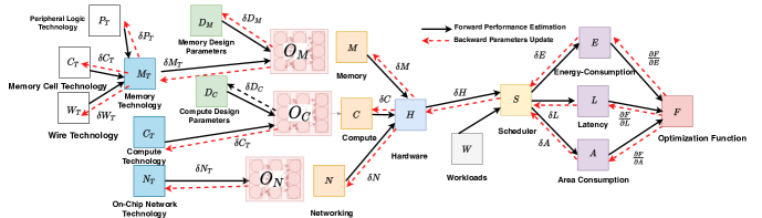
Figure 2: Forward and Backward Phase Execution

3 The Hardware Model

Parameter Type	Value	Classes	Parameter Names
CompTechPars	$\mathcal{R}$	$cc\in CompCls$	${\color[rgb]{0.921875,0.30078125,0.29296875}{\texttt{wireCap}}},{\color[rgb]{0.921875,0.30078125,0.29296875}{\texttt{wireResisist}}}$
	$\mathcal{Z}$		node
MemTechPars	$\mathcal{R}$	$mc\in MemCls$	${\color[rgb]{0.921875,0.30078125,0.29296875}{\texttt{wireCap}}},{\color[rgb]{0.921875,0.30078125,0.29296875}{\texttt{wireResist}}}$
			${\color[rgb]{0.921875,0.30078125,0.29296875}{\texttt{cellReadLatency}}},{\color[rgb]{0.921875,0.30078125,0.29296875}{\texttt{cellAccessDevice}}}$
			${\color[rgb]{0.921875,0.30078125,0.29296875}{\texttt{cellReadPower}}},{\color[rgb]{0.921875,0.30078125,0.29296875}{\texttt{cellLeakagePower}}}$, cellArea
	$\mathcal{Z}$		peripheralLogicNode
CompArchPars	$\mathcal{Z}$	systolicArray	sysArrX,sysArrY, sysArrN
		vector	${\color[rgb]{0.921875,0.30078125,0.29296875}{\texttt{vectDataWidth}}},{\color[rgb]{0.921875,0.30078125,0.29296875}{\texttt{vectN}}}$
		macTree	${\color[rgb]{0.921875,0.30078125,0.29296875}{\texttt{mTreeX}}},{\color[rgb]{0.921875,0.30078125,0.29296875}{\texttt{mTreeY}}},{\color[rgb]{0.921875,0.30078125,0.29296875}{\texttt{mTreeTileX}}},{\color[rgb]{0.921875,0.30078125,0.29296875}{\texttt{mTreeTileY}}}$
		fpu	fpuN
		SoC	frequency
MemArchPars	$\mathcal{Z}$	$mc\in MemCls$	${\color[rgb]{0.921875,0.30078125,0.29296875}{\texttt{capacity}}},{\color[rgb]{0.921875,0.30078125,0.29296875}{\texttt{bankSize}}},{\color[rgb]{0.921875,0.30078125,0.29296875}{\texttt{nReadPorts}}}$
CompMetrics	$\mathcal{R}$	$cc\in CompCls$	${\color[rgb]{0.921875,0.30078125,0.29296875}{\texttt{intPower}}},{\color[rgb]{0.921875,0.30078125,0.29296875}{\texttt{leakagePower}}},{\color[rgb]{0.921875,0.30078125,0.29296875}{\texttt{latency}}},{\color[rgb]{0.921875,0.30078125,0.29296875}{\texttt{area}}}$
MemMetrics	$\mathcal{R}$	$mc\in MemCls$	${\color[rgb]{0.921875,0.30078125,0.29296875}{\texttt{readLatency}}},{\color[rgb]{0.921875,0.30078125,0.29296875}{\texttt{writeLatency}}}$
			${\color[rgb]{0.921875,0.30078125,0.29296875}{\texttt{readEnergy}}},{\color[rgb]{0.921875,0.30078125,0.29296875}{\texttt{writeEnergy}}}$
			${\color[rgb]{0.921875,0.30078125,0.29296875}{\texttt{leakagePower}}},{\color[rgb]{0.921875,0.30078125,0.29296875}{\texttt{area}}}$

Table 2: Summary of compute and memory technology parameters, architectural parameters, and performance metrics. Each parameter is mapped to either a real or a natural number in a concrete hardware model. Some parameters only apply for a particular hardware unit.

The hardware model captures the performance of a class of candidate hardware designs. The hardware model models the performance of each memory unit $mc\in MemCls{}=\{{\color[rgb]{0.921875,0.30078125,0.29296875}{\texttt{localMem}}},{\color[rgb]{0.921875,0.30078125,0.29296875}{\texttt{globalBuf}}},{\color[rgb]{0.921875,0.30078125,0.29296875}{\texttt{mainMem}}}\}$ and each compute unit $cc\in CompCls{}=\{{\color[rgb]{0.921875,0.30078125,0.29296875}{\texttt{systolicArray}}},{\color[rgb]{0.921875,0.30078125,0.29296875}{\texttt{vector}}},{\color[rgb]{0.921875,0.30078125,0.29296875}{\texttt{macTree}}},{\color[rgb]{0.921875,0.30078125,0.29296875}{\texttt{Fpu}}}\}$ in the hardware design. Together, the memory units and compute units make up the hardware units in the hardware design $c\in HwCls=CompCls\cup MemCls$.

Architectural and Technology Parameters: The hardware model is defined over a set of technology parameters $tp{}\in TP{}\subset TechPars{}$ and architectural parameters $ap{}\in AP{}\subset ArchPars{}$ that capture the technology-specific and architectural properties that can be tuned at design-time. Each of the technology and architectural parameters resolve to real numbers $x\in\mathcal{R}$ when the hardware model is specialized to implement a specific design.

Table 2 presents a summary of the memory and compute technology parameters and architectural parameters. The technology parameters are broken up into memory technology parameters ($MemTechPars$) that capture the characteristics of memory devices, and compute primitive technology parameters ($CompArchPars$) that capture the characteristics of computational primitives, such as flip-flops, adders, and multipliers. The architectural parameters $ArchPars=CompArchPars\cup MemArchPars$ are broken up into memory architectural parameters ($MemArchPars$) and compute architectural parameters $CompArchPars$. Some architectural parameters only apply to a particular kind of compute unit.

Metrics: The hardware model models the following the compute and memory performance metrics $m\in M=MemMetrics\cup CompMetrics$ for each memory and compute unit in the design. Table 2 summarizes the memory and compute unit metrics captured in the hardware model.

The Hardware Model: The hardware model models each performance metric as a differentiable, algebraic function $e\in E\subseteq Exprs$ over technology parameters $tp{}\in TP{}\subset TechPars{}$ and architectural parameters $ap{}\in AP{}\subset ArchPars{}$. The hardware model is fully described as follows:

$$\texttt{\color[rgb]{0.28125,0.203125,0.83203125}{H}}\in HwModels=(CompCls\times CompMetrics)\cup(MemCls\times MemMetrics)\rightarrow Exprs$$

The hardware model maps pairs of compute and memory class-metric pairs to architecture- and technology-parameter dependent expressions. To derive a concrete hardware model that captures the performance of a specific hardware design from the above model, we apply a set of technology parameter assignments $TA\subseteq\mathcal{P}(TechPars{}\times\mathcal{R})$ and a set of architectural parameter assignments $AA{}\subseteq\mathcal{P}(ArchPars{}\times\mathcal{Z})$ to the mapped expressions:

$$\texttt{\color[rgb]{0.28125,0.203125,0.83203125}{CH}}=\texttt{\color[rgb]{0.28125,0.203125,0.83203125}{specialize}}(\texttt{\color[rgb]{0.28125,0.203125,0.83203125}{H}},TA{},AA{})=\{\langle c,m\rangle\rightarrow\texttt{\color[rgb]{0.28125,0.203125,0.83203125}{sub}}(e,TA\cup AA)~{}|~{}\texttt{\color[rgb]{0.28125,0.203125,0.83203125}{H}}(\langle c,m\rangle)=e\}$$

The concrete hardware model $\texttt{\color[rgb]{0.28125,0.203125,0.83203125}{CH}}\in ConcHwModels=(CompCls\times CompMetrics)\cup(MemCls{}\times MemMetrics)\rightarrow\mathcal{R}$ maps the compute and memory performance metrics for each compute and memory unit to real values.

4 Application Workloads

The DRAGON toolchain works with application workloads $w\in W\subseteq Workloads$. Each workload is provided as a dataflow graph or a control dataflow graph. Each workload $w$ is a directed graph with a list of vertices $v\in Verts$ and a list of edges $e\in Edges$.

5 DRAGON

We introduce DRAGON, a suite of hardware simulation and optimization tools that enable hardware designers to simulate hardware designs, and to optimize hardware designs to efficiently execute certain workloads. The DRAGON toolchain provides the following tools:

• Hardware Model Generator (DGen, Section 5.1): DGen derives a hardware model H from an architectural specification that describes the overall structure of the hardware platform. DGen works with a device model library that models the performance metrics for each computational primitive (flip-flop, adder, and multiplier) and memory unit, and an accelerator template library that derives the performance models for each type of computational unit $cc$ in the architectural specification. The accelerator library uses the computational primitive performance models from the device model library to derive the computational unit models. The output of DGenis a hardware model H that models the performance of the provided hardware design.

• Hardware Simulator (DSim, Section 6): DSimproduces performance estimates for a concrete hardware design. DSim takes as input a concrete hardware model CH and a computational workload $w$ and derives energy, power, runtime, and area measurement estimates. The output of the hardware simulator is a set of performance estimate $\texttt{\color[rgb]{0.28125,0.203125,0.83203125}{P}}\in PerfEstimate:Measurements\rightarrow\mathcal{R}^{+}$, where $q\in Measurements=\{{\color[rgb]{0.921875,0.30078125,0.29296875}{\texttt{energy}}},{\color[rgb]{0.921875,0.30078125,0.29296875}{\texttt{power}}},{\color[rgb]{0.921875,0.30078125,0.29296875}{\texttt{area}}},{\color[rgb]{0.921875,0.30078125,0.29296875}{\texttt{runtime}}}\}$.

• Hardware Optimizer (DOpt, Section 7) DOptoptimizes the technology and architectural parameters in a given hardware design so that the hardware design efficiently executes a set of workloads. DOpt takes as input a hardware model H, a set of initial technology and architectural parameter assignments $TA$ and $AA$, and a collection of computational workloads $W$ and produces as output a set of technology and architectural parameter assignments $TA^{\prime}$ and $AA^{\prime}$ that optimize the performance of the hardware on the provided set of workloads. We also present an extension to DOpt, $Dopt2$, that also optimizes the architectural specification used to derive the hardware model to optimally execute the candidate workloads.

5.1 Hardware Model Generator (DGen)

The DGen hardware model generator accepts as input a specification of the hardware architecture, a device-level performance model library and a template library for different accelerator designs:

• Architectural Specification: The architectural specification $a\in A=\mathcal{P}(MemCls)\times\mathcal{P}(CompCls)\times{MemCls\rightarrow MemTypes}$ selects the subset of memory units and compute units present in the hardware platform and assigns each memory unit to a memory type $\texttt{\color[rgb]{0.28125,0.203125,0.83203125}{memType}}\in memAssignFuncs:MemCls\rightarrow MemTypes$. The memory type of each memory unit $mt\in MemTypes=\{{\color[rgb]{0.921875,0.30078125,0.29296875}{\texttt{sram}}},{\color[rgb]{0.921875,0.30078125,0.29296875}{\texttt{rram}}},{\color[rgb]{0.921875,0.30078125,0.29296875}{\texttt{dram}}}\}$ determines which device performance models to use.

• Device Performance Model Library: The device performance model library contains a library of performance models for different memory technologies $\texttt{\color[rgb]{0.28125,0.203125,0.83203125}{memLib}}\in DevMemLib:MemTypes\times MemMetrics\rightarrow Exprs$ and a library of performance models for different logical primitives $\texttt{\color[rgb]{0.28125,0.203125,0.83203125}{primLib}}\in DevPrimLib:PrimitiveType\times CompMetrics\rightarrow XExprs$, where the logical primitives in the model library are $PrimitiveType=\{{\color[rgb]{0.921875,0.30078125,0.29296875}{\texttt{adder}}},{\color[rgb]{0.921875,0.30078125,0.29296875}{\texttt{ff}}},{\color[rgb]{0.921875,0.30078125,0.29296875}{\texttt{mult}}}\}$. Here, $xe\in XE\subset XExprs$ define the space of expressions over only technology parameters.

• Accelerator Template Library: The accelerator template library derives the compute unit performance models from the performance models of different logical primitives. The $\texttt{\color[rgb]{0.28125,0.203125,0.83203125}{accTempls}}:\texttt{\color[rgb]{0.28125,0.203125,0.83203125}{primLib}}\times CompCls\times CompMetrics\rightarrow Exprs$.

DGen produces as output, a hardware performance model H that is then used by the DRAGON simulator and optimizer to simulate and optimize the hardware design.

5.1.1 Deriving the Hardware Model

Given an architectural specification $\langle MC,CC,\texttt{\color[rgb]{0.28125,0.203125,0.83203125}{memType}}{}\rangle$ and the device memory model memLib, DGen derives a an expression $e$ for each memory performance metric $mm$ and each memory unit $mc\in MC$:

$$\texttt{\color[rgb]{0.28125,0.203125,0.83203125}{H}}(mc,mm):=\texttt{\color[rgb]{0.28125,0.203125,0.83203125}{memLib}}(\texttt{\color[rgb]{0.28125,0.203125,0.83203125}{memType}}(mc),mm)$$

Given an architectural specification $\langle MC,CC,\texttt{\color[rgb]{0.28125,0.203125,0.83203125}{memType}}\rangle$, the logical primitive performance models primLib, and the accelerator template library accTempls, DGen derives an expression $e$ for each compute performance metric $cm$ and each compute unit $cc\in CC$:

$$\texttt{\color[rgb]{0.28125,0.203125,0.83203125}{H}}(cc,cm):=\texttt{\color[rgb]{0.28125,0.203125,0.83203125}{accTempls}}(\texttt{\color[rgb]{0.28125,0.203125,0.83203125}{primLib}},cc,cm)$$

5.2 Software Stack Simulation

Algorithm 1 Software Stack Simulation

1:function prefetchVertex(CH, $z$, $ms$, $cs$, $V$,$VS$)

2:    match $V,VS$ do

3:        case $[],[]$

4:           return simulateVertex(CH,$z$,$ms$, $cs$, $V$, $VS$)         

5:        case $v::V^{\prime},vs::VS^{\prime}$

6:           $nComp,nAlloc,nRead,nWrite=\texttt{\color[rgb]{0.28125,0.203125,0.83203125}{getStats}}(vs)$

7:           if hasSpace(CH, nAlloc) then

8:               $ms^{\prime},vs^{\prime}$ = prefetch($v$,$vs$, $ms)$

9:               return mapVertex(CH,$z$,$ms^{\prime}$, $cs$, $v::V$, $vs^{\prime}::VS$)

10:           else

11:               return mapVertex(CH,$z$,$ms$, $cs$, $V$, $VS$)

12:           end if            

13:end function

14:function mapVertex(CH, $z$, $ms$, $cs$, $V$,$VS$)

15:    match $V,VS$ do

16:        case $[],[]$

17:           return $\langle z,ms,cs\rangle$         

18:        case $v::V^{\prime},vs::VS^{\prime}$

19:           $nComp,nAlloc,nRead,nWrite=\texttt{\color[rgb]{0.28125,0.203125,0.83203125}{getStats}}(vs)$

20:           if $\neg~{}\texttt{\color[rgb]{0.28125,0.203125,0.83203125}{hasSpace}}$(CH, nAlloc) then

21:               $v^{\prime},v^{\prime\prime}=\texttt{\color[rgb]{0.28125,0.203125,0.83203125}{splitVertex}}(v)$

22:               $vs^{\prime},vs^{\prime\prime}=\texttt{\color[rgb]{0.28125,0.203125,0.83203125}{getVertexState}}(\texttt{\color[rgb]{0.28125,0.203125,0.83203125}{CH}},[v^{\prime},v^{\prime\prime}])$

23:               return mapVertex(CH, $z$, $ms$, $cs$, $v^{\prime}::v^{\prime\prime}::V^{\prime}$,$vs^{\prime}::vs^{\prime\prime}::VS^{\prime}$)

24:           else

25:               $z^{\prime}$,$cs^{\prime}$ = mapToCompute(CH, $cs$, nComp)

26:               $ms^{\prime}$ = memAlloc(CH,$ms$, nAlloc)

27:               $ms^{\prime\prime}$ = mapMemAcc(CH,$ms^{\prime}$,nRead,nWrite)

28:               return prefetchVertex(CH, $z^{\prime}$, $cs^{\prime}$, $ms^{\prime\prime}$, $V^{\prime}$, $VS^{\prime}$)

29:           end if             

30:end function

31:function mapWorkload($w$, CH)

32:    $\langle V,E\rangle=\texttt{\color[rgb]{0.28125,0.203125,0.83203125}{workloadOptimize}}(w)$

33:    $VS$ = $\texttt{\color[rgb]{0.28125,0.203125,0.83203125}{getVertexState}}(\texttt{\color[rgb]{0.28125,0.203125,0.83203125}{CH}},V)$

34:    $ms=\{mc\to\langle 0,0,0,0\rangle~{}|~{}mc\in MemCls\}$

35:    $cs=\{cc\to\langle 0,0,0\rangle~{}|~{}cc\in CompCls\}$

36:    return mapVertex(CH,0,$ms$, $cs$)

37:end function

The mapper maps the workload to the concrete hardware specification. The algorithm optimizes the workload on the fly to execute efficiently on the target hardware platform an estimates the performance of the workload on the target hardware platform. The mapper algorithm is used by DSim to estimate the performance of the workload on the hardware, and is used by the DOpt to optimize the hardware parameters to efficiently execute the target computation. The mapper performs the three basic operations:

• mapWorkload: Map the workload to the concrete hardware specification. The algorithm optimizes the workload on the fly to execute efficiently on the target hardware platform an estimates the performance of the workload on the target hardware platform.

• mapVertex: Map a single DFG node to the target hardware, as described by the concrete hardware specification. The algorithm returns the updated memory state, compute state, and vertex state of the hardware platform. The the target node consumes more memory than is available, the mapper applies a memory streaming optimization that reduces the amount of memory that needs to be allocated (lines 20-23). Otherwise, the mapper applies a prefetching compiler optimization (prefetchVertex) and continues executing the program.

• prefetchVertex: Emulates a prefetching compiler optimization (XXX).

The mapper tracks the following additional quanitites:

• Vertex State: The vertex state captures the resource utilization of a DFG vertex on the hardware described in the concrete hardware specification. The vertex state tracks the number of compute operations performed on each compute unit, the number of read accesses performed on each memory unit, and the number of write accesses and allocations for each memory unit. The vertex state is used to up

• Memory State: The memory state tracks the amount of memory utilized, the memory bandwidth utilized, the number of rows utilized, and number of columns utilized for each memory unit in the concrete hardware specification.

• Compute State: The compute state tracks the number of cores utilized. If the compute unit is a systolic array, the first and second values track the number of rows and columns utilized.

• Cycle Count: The algorithm tracks the cycle count.

The mapper makes use of the following helper functions:

• getStats: get the total number of allocations, total number of reads, and total number of writes performed by the vertex state.

• splitVertex: Split the workload vertex into two vertices.

• hasSpace: Return if the concrete hardware specification has enough space to allocate $nAlloc$ bytes.

• getVertexState: Get the vertex state for the vertex, given the concrete hardware specification.

• workloadOptimize: optimize the order the vertices and edges should be visted in the workload. Returns the optimized workload. Models compiler optimizations such as DFG partitioning, Compute Merge Optimizer.

The mapper uses the following functions to estimate the performance of the workload on the hardware. These functions have some XXX property XXX that enables them to be differentiated:

• mapToCompute: updates the compute state to perform $nComp$ compute operations on the target hardware.

• memAlloc: updates the memory state to perform $nAlloc$ allocations in the memory hierarchy.

• mapMemAcc: updates the memory state to perform $nRead$ reads and $nWrite$ writes on teh stored data.

• prefetch: Emulates prefetching

5.3 The DSim Simulator

Runtime: The DSim simulator calculates the runtime from $z$, the number of cycles returned by mapWorkload and the frequency architectural parameter from the architectural specification:

$$Runtime=z\cdot\texttt{\color[rgb]{0.28125,0.203125,0.83203125}{CH}}({\color[rgb]{0.921875,0.30078125,0.29296875}{\texttt{SoC}}},{\color[rgb]{0.921875,0.30078125,0.29296875}{\texttt{frequency}}})$$ (1)

Energy: The DSim simulator calculates the energy from the memory state $ms$ and compute state $cs$ returned by the mapWorkload algorithm, and the $mm$ and $cm$ metrics from the concrete hardware specification. Each of these metrics resolves to a real value in the concrete hardware specification.

Energy = 0

for $mc\in MemCls$ do

    $\_,\_,reads,writes=ms(mc)$

    $re,we,lp=mm(mc)$

    $Energy+=\sum_{i}^{N}reads\times re+writes\times we+lp\times Runtime$

end for

for $cc\in CompCls$ do

    $\_,\_,num\_access=cs(cc)$

    ${}_{,}en,lp=cm(cc)$

    $Energy+=\sum_{i}^{N}en\times num\_access+lp\times Runtime$

end for

Compact Representation: The total energy consumption is $Energy_{mem}+Energy_{compute}$, the sum of the energy consumption from the memory units, and the energy consumption from the compute units.

$$Energy_{mem}=\sum_{mc\in MemCls} \texttt{\color[rgb]{0.28125,0.203125,0.83203125}{CH}}(mc,{\color[rgb]{0.921875,0.30078125,0.29296875}{\texttt{readEnergy}}})\cdot r+\texttt{\color[rgb]{0.28125,0.203125,0.83203125}{CH}}(mc,{\color[rgb]{0.921875,0.30078125,0.29296875}{\texttt{writeEnergy}}})\cdot w$$

$$+\texttt{\color[rgb]{0.28125,0.203125,0.83203125}{CH}}(mc,{\color[rgb]{0.921875,0.30078125,0.29296875}{\texttt{leakagePower}}})\cdot Runtime$$

$$\textbf{where}\langle\_,r,w\rangle=ms(mc)$$

$$Energy_{compute}=\sum_{cc\in CompCls} \texttt{\color[rgb]{0.28125,0.203125,0.83203125}{CH}}(cc,{\color[rgb]{0.921875,0.30078125,0.29296875}{\texttt{intEnergy}}})\cdot numAcc+\texttt{\color[rgb]{0.28125,0.203125,0.83203125}{CH}}(cc,{\color[rgb]{0.921875,0.30078125,0.29296875}{\texttt{leakagePower}}})\cdot Runtime$$

$$\textbf{where}~{}\langle\_,\_,numAcc\rangle=cs(cc)$$

Area: The area of the hardware platform is the sum of all the areas of the compute units and the sym of all the areas of the memory units.

$$Area=\sum_{mc\in MemCls}\texttt{\color[rgb]{0.28125,0.203125,0.83203125}{CH}}(mc,{\color[rgb]{0.921875,0.30078125,0.29296875}{\texttt{area}}})+\sum_{cc\in CompCls}\texttt{\color[rgb]{0.28125,0.203125,0.83203125}{CH}}(cc,{\color[rgb]{0.921875,0.30078125,0.29296875}{\texttt{area}}})$$ (2)

Power: The power is the average energy over the runtime.

$$Power=Energy/Runtime$$ (3)

6 Hardware Simulator (DSim)

The hardware simulator DSim accepts as input a concrete hardware model CH and workload to simulate $w$ and produces as output a collection of performance estimates P that report the latency, energy, power, and area of the hardware.

Algorithm 2 DSim simulation algorithm

1:function simulate($w$, CH)

2:    $ms=\{mc\to\langle 0,0,0,0\rangle~{}|~{}mc\in MemCls\}$

3:    $cs=\{cc\to\langle 0,0,0\rangle~{}|~{}cc\in CompCls\}$

4:    $\langle V,E\rangle=\texttt{\color[rgb]{0.28125,0.203125,0.83203125}{workloadOptimize}}(w)$

5:    $VS$ = computeVertexState(V)

6:    nCycles = 0

7:    for $v_{i}::V$, $vs_{i}::VS$ do

8:        $nComp,nAlloc,nRead,nWrite=\texttt{\color[rgb]{0.28125,0.203125,0.83203125}{getStats}}(vs_{i})$

9:        if $\neg~{}hasEnoughSpace$(CH, nAlloc) then

10:           $v_{i}^{\prime},v_{i}^{\prime\prime}=split(v_{i})$

11:           $vs_{i}^{\prime},vs_{i}^{\prime\prime}$ = ComputeVertexState($v_{i}^{\prime}$),ComputeVertexState($v_{i}^{\prime\prime}$)

12:           $V=v_{i}^{\prime}::v_{i}^{\prime\prime}::[v_{i_{1}}...v_{N}]$

13:           $VS=vs_{i}^{\prime}::vs_{i}^{\prime\prime}::[..XXX...]$

14:        else

15:           cycles,$cs^{\prime}$ = maptoCompute(CH, nComp)

16:           $ms^{\prime}$ = memAlloc(CH,$ms$, nAlloc)

17:           $ms^{\prime\prime}$ = applyMemAccesses(CH,$ms^{\prime}$,nRead,nWrite)

18:        end if

19:        nCycles += cycles

20:        $\_,nAlloc^{\prime},\_,\_=\texttt{\color[rgb]{0.28125,0.203125,0.83203125}{getStats}}(v_{i+1})$

21:        if hasEnoughSpace(CH, nAlloc’) $\wedge$ $i+1<||V||$ then

22:           $ms^{\prime\prime\prime},vs_{i+1}^{\prime}$ = Prefetch($v_{i+1}$, $vs_{i+1}$, ms”)

23:           $VS[i+1]=vs_{i+1}^{\prime}$

24:           cs,ms= cs’,ms”’

25:        else

26:           cs,ms= cs’,ms”

27:        end if

28:    end forreturn $\langle nCycles,cs,ms\rangle$

29:end function

Vertex State: Each vertex has state, $vertexstate$.

State: The simulator maintains the state of the hardware while executing the computation. The hardware state is broken up into memory $ms$ and the compute sate $cs$.

Memory State: Memory capacity utilization [Natural], Bandwidth utilization [Natural] (2 values) Compute: utilization for number of rows and number of columns in NxM dimensional compute fabric. For XXX, YYY, ZZZ the dimension M = 1, so the second tuple value is always zero. For systolic array, both values can be non-zero. Order for memory state [capacity utilization, bandwidth utilization, numberReads, numberWrites]. Order for compute is going to be [number compute operations, number rows activated, number columns activated].

Statistics: For each vertex we collect the number of cycles, number of compute operations, and the number of read accesses and write accesses. As we traverse the graph, we track the number of cycles (cycles), number of compute operations (nComp, per compute unit), number of read accesses (nRead, per memory unit), and number of write accesses (nWrite, per memory unit). All of these values are natural nubmers.

7 The DOpt Optimizer

The mapping/scheduling process prevent differentiation of the mapping process.

Since, different scheduling algorithms create a large number of hardware components, a technology-to-component bipartite graph is created with gathers the technology parameter updates from the hardware components.

The derivatives “flow” backwards from the performance objective specified to the design and technology parameters after our techniques that make the scheduling and mapping process differentiable.

The first sub-process of the backward produces the optimal accelerator designs : 1. Optimizing the accelerator given for mapping and 2. Optimizing the accelerator design generation from scheduling (i.e. creating a performance objective aware binding process and finding parameters of loop unrolling, pipelining, memory divisions, etc).

In the second sub-process the technology parameters are updated, via the gradient flows from the differentiable component models in our framework. From the updated technology parameters, the characteristics of the component models in hardware description are modelled again for the subsequent forward pass,

One iteration of forward and backward pass (where the design/tech params are updated), constitutes a single epoch of our framework. This process is iterated for several epochs until either a convergence of the parameters is reached (for accelerator design params) or the performance benefit objective is met (for technology parameters).

Using our backward pass, we plot gradient updates of the design and technology parameters, Figure 3 shows the design and technology parameter space, the gradient flows are demonstrated with little arrows.

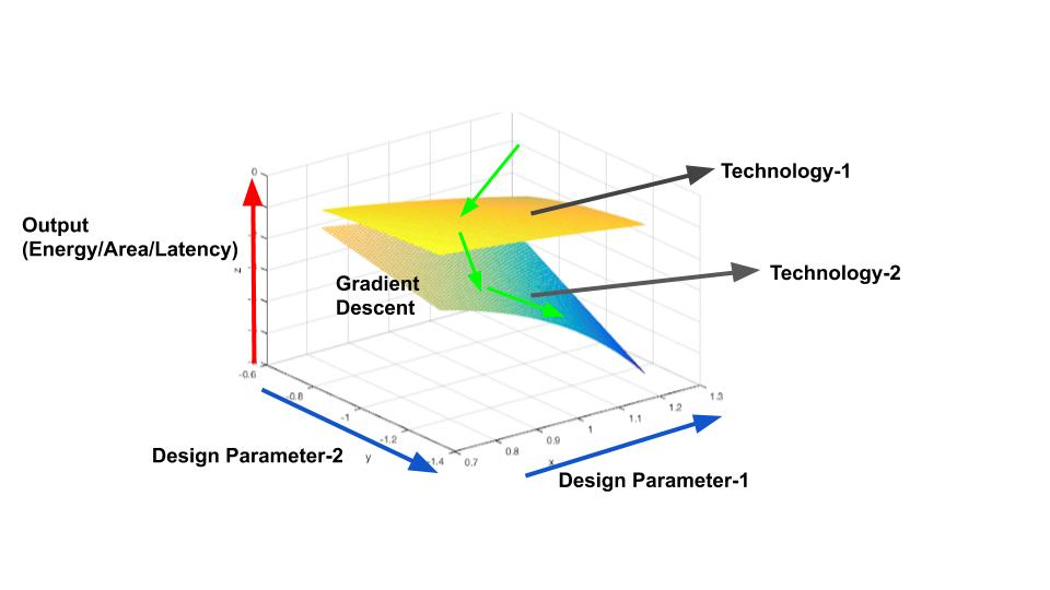
Figure 3: Gradient Descent Optimization on the Joint Space of Design and Technology Params

8 Discussion and Results

8.1 Execution Speed and Validation Results

Figure 1 shows that our estimates are simultaneously accurate (within 80-97% accuracy) and fast ( 1,000-fold faster, 1 second vs 30 mins. per simulation run) compared to state-of-the-art simulators (such as SCALE-Sim, NN-Dataflow, ZigZag) for a wide range of (AI) Workloads (CNNs, LSTMs, DLRMs, Transformers).

In addition, our framework is readily available (vs. several months of development time for state-of-the-art accelerators) for performance estimation on new classes of AI-workloads and accelerators.

Figure shows the accuracy comparison of our Hardware Simulator compared to open source frameworks available (Scale-Sim, Timeloop, Zigzag) and cycle accurate simulators such as N3XT Sim.

8.2 Design Space Exploration Results

Table 4 shows the optimal architecture derived from the exploration of AI and Non-AI workloads, and the gradient descent curves for design parameters are shown in Figure 7.

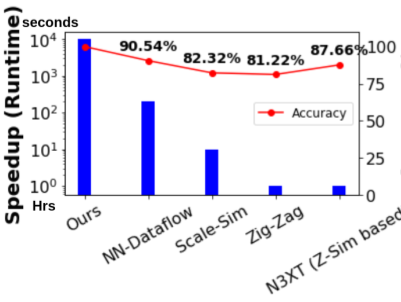
Figure 4: Accuracy of Our Framework with Existing Works

8.3 Technology Derivation Results

Table 5 shows the technology targets required for workloads

Figure 3 shows the technology targets derived for 100X EDP performance of Google’s BERT, and the order in which those technology targets improvement need to be executed. Targeting different technology parameters the EDP benefits decrease considerably to 1.82X (as in Figure 3(b)). The execution time of our framework in deriving these technology targets is within 10s, while an iterative approach over several technology space points ($>10^{5}$) in a simulation run will take a time frame of weeks.

Inference/Training	Objective : Execution Time	Objective : Energy Consumption
Vision Models	On chip memory density $\geq$ Connectivity $>$
	External memory frequency $>$
	Wire capacitance $>$ Logic delay	Logic energy $>$ External Memory: Cell leakage $>$
		External/Internal memory Peripheral logic leakage
Language Models	Connectivity $>$ On chip memory density $>$
	external memory frequency $>$
	Wire capacitance $>$ Logic delay	On chip memory: Wire cap. $>$
		External memory: Cell leakage $>$ Logic energy $>$
		On chip memory cell leakage
Recommendation Models	Connectivity	Connectivity$>$  On chip memory : peripheral logic cap

Table 3: Order of Importance for Different Technologies

9 Software Availability

The code is available at https://github.com/missionfission/dragon-project, released under the CC BY 4.0 license.

10 Appendix A : Algorithms

Algorithm 3 Data-flow Graph Optimizations

1:Compute Merge Optimizer

2:Merges small nodes in parallel to execute more efficiently

3:DFG = D(V, E) denote the input workload data flow graph,

4:Create a new DFG/set of DFG’s

5:$D’=bridgepartition(D)={D_{1}(V,E),D_{2}(V,E),D_{3}(V,E)...}$

6:for d do $\in\ D^{\prime}$

7:    p = $source-cut(d)$

8:    for $p_{1},p_{2}...\in p$ do

9:        if $p_{1}.compute<H_{vth}$ and $p_{2}.compute<H_{vth}$ and .., $\sum p_{i}.compute<H_{vth}$ then,

10:           p’ = merge ($p_{1}$ , $p_{2}$ ..) ..

11:        end if

12:    end for

13:end forreturn D’

Algorithm 4 Scheduling Backpropagation

1:D(V,E) for execution

2:Architecture Generation and Execution (Scheduling, Allocation and Binding).

3:Identify parameter points, for ex. Memory partitioning, loop unrolling, etc. (can be given externally for fixed hardware).

4:AD = $P_{i}$ (Accelerator design space is the set of all parametric points)

5:for node n in D(V, E) :  do

6:    $T_{exec}=t_{max}(t_{mem}\_M_{i},..,t_{c}\_C_{i})$

7:    $T_{exec_{m}in}=t_{min}(t_{mem}\_M_{i},..,t_{c}\_C_{i})$

8:    $E_{exec}=E_{mem}\_M_{i}+E_{c}\_C_{i}$

9:    $T_{total}+=t_{exec}$

10:    $E_{total}+=E_{exec}$ 

11:    $T_{gradient}\_M_{i}+=t_{min}-t_{mem}\_M_{i}$

12:    $T_{gradient}\_C_{i}+=t_{min}-t_{c}\_C_{i}$

13:    $E_{gradient}\_M_{i}=E_{mem}\_M_{i}$

14:    $E_{gradient}\_C_{i}=E_{c}\_C_{i}$ $f(..M_{i}..)=t_{mem}\_M_{i}$

15:end for

16:if (perf objective = time) then

17:    $M_{i}=-\alpha*T_{gradient}\_M_{i}/(\delta M_{i})(\delta M_{i}=\frac{\partial P}{\partial M_{i}})$

18:end if

19:if ( thenperf objective = energy)

20:    $M_{i}=-\alpha*E_{gradient}\_M_{i}/(\delta M_{i})(\delta M_{i}=\frac{\partial P}{\partial M_{i}})$

21:end if

Algorithm 5 Template-Space Mapping Backpropagation

1:AD = $P_{i}$ (Accelerator design space is the set of all parametric points)

2:for node n in D(V, E) do :

3:    Node.in_edges = []

4:    compute_time(in_edges)

5:    partitioned nodes, $T_{exec}=fractional\_exec(t_{max}(t_{mem}\_M_{i},..,t_{c}\_C_{i})+in_{o}ut\_swap_{t}ime)$

6:    $T_{exec}=t_{max}(t_{mem}\_M_{i},..,t_{c}\_C_{i})$

7:    $T_{exec}\_min=t_{min}(t_{mem}\_M_{i},..,t_{c}\_C_{i})$

8:    $E_{exec}=E_{mem}\_M_{i}+E_{c}\_C_{i}$

9:    $T_{total}+=t_{exec}$

10:    $E_{total}+=E_{exec}$

11:    $T_{gradient}\_M_{i}+=t_{min}-t_{mem}\_M_{i}$

12:    $T_{gradient}\_C_{i}+=t_{min}-t_{c}\_C_{i}$

13:    $E_{gradient}\_M_{i}=E_{mem}\_M_{i}$

14:    $E_{gradient}\_C_{i}=E_{c}\_C_{i}$ For memory size : $f(..M_{i}..)=t_{mem}\_M_{i}$

15:    if ( thenperf objective = time)

16:        $M_{i}=-\alpha*T_{gradient}\_M_{i}/(\delta M_{i})(\delta M_{i}=\frac{\partial P}{\partial M_{i}}$

17:    end if

18:    if ( thenperf objective = energy)

19:        $M_{i}=-\alpha*E_{gradient}\_M_{i}/(\delta M_{i})(\delta M_{i}=\frac{\partial P}{\partial M_{i}})$

20:    end if

21:    Total Memory Energy Consumption (TMEC) : $\sum_{i}$ (${ww}_{M_{i}}$ *${ew}_{M_{i}}$ + ${rw}_{M_{i}}$*${er}_{M_{i}}$ + $l_{M_{i}}*t_{W}$) where, Dynamic read energy (nJ) : ${er}_{M_{i}}$, Dynamic write energy (nJ): ${ew}_{M_{i}}$, Standby leakage per bank(mW) : $l_{M_{i}}$, Read Accesses : ${rw}_{M_{i}}$, Write Accesses : ${ww}_{M_{i}}$, Workload Execution Time : $t_{W}$, So, individual gradients are,

$$\delta({ew}_{M_{i}})=\delta(TMEC)/({ww}_{M_{i}})$$ (4)

$$\delta({rw}_{M_{i}})=\delta(TMEC)/({er}_{M_{i}})$$ (5)

$$\delta({l_{M_{i}}})=\delta(TMEC)/({t_{W}})$$ (6)

$$\delta({t_{W}})=\sum_{i}\delta(TMEC)/({l_{M_{i}}})+\sum_{i}\delta(TMEC)/({l_{C}})$$ (7)

22:end for

Algorithm 6 Full Flow of Backward Pass

1:Start with a generated/random Hardware point $\to$ Nodes of the graph are scheduled

2:Do the Scheduling with that Point $\to$ Generate the Execution Statistics (Component-breakdown of the area, energy, and timing) Generate the reference tables using plugins $\to$ Currently using a table at 40nm.

3:Generate Logs of the memory states variations i.e. memory bandwidth and utilization over the execution of the graph. (Extreme use high/low memory bandwidth requirements and high/low memory utilization)

4:Apply Gradient Descent on the Optimization metric (time/area/energy/edp)

5:Update the hardware config $\to$ Check the values are realistic (within a certain bound).

6:Iterate until convergence. Checkout if performance at constraint boundaries is better.

11 Appendix B : Mapping, Scheduling and Synthesis Details

Algorithm 7 Prefetch nodes

1:D = list(n in sorted_nodes())

2:for n in D: do

3:    if mem.bw_util $>$ 0.9*bw_limit : then

4:        continue

5:    end if

6:    if mem.size_util $>$ 0.9*size_limit & mem_bw $<$ 0.9*bw_limit then

7:        n.set_execution = streaming

8:    end if

9:    if mem.size_util $<$ 0.9*size_limit & mem_bw $<$ 0.9*bw_limit then

10:        n.next.fetch_data()

11:    end if

12:end for

11.0.1 Mapping for Performance Objective

For the objective of fastest execution/(execution time), we follow the above strategy of prefetching nodes and tiling for highest execution time.

For execution of a application, that consumes lower energy consumption, the strategies used are to somehow lower the computational and memory accesses for the application.

Finding Compute-Reuse/Data-Reuse Oppurtunities in Applications

• Reducing memory accesses by storing commonly reused data in a buffer, so that it can be accessed again for consumption. Identifying locality is expressed in two ways : Spatial and Temporal Locality. Taking advantage of data reuse opportunities is possible, if the corresponding stall caused by data reuse, such as reduced bandwidth access to the compute blocks is mitigated by the schedule.

  Stencil Data Reuse : Data reuse in common stencils is possible, analytical expressions for quantifying of data reuse of matrix multiplication, simple linear algebra processing.

  Loop Blocking : Convolution Loop blocking [17] describes the locality for allowing efficient data reuse in convolutional workloads, by an exhaustive search of the loop orderings. We formulate the loop ordering search for energy efficiency as similar problem, and solve the tiling parameter search using gradient descent optimization.

  $${x,y,c,k}=min(energy\_cost(loop\_tiling(x,y,c,k)))$$ (8)

  where x = [x_1,x_2 ..] for n memory levels. Data reuse opportunities existing in general applicatons is found using Reduction trees (finding source-cycles in DFG in a certain time-frame) described in [3, 8]

• The second strategy is to stored the result of computation of commonly used sub-expressions, that utilize the same data in the memory buffer space, this can reduce energy consumption of the map(application $\to$ hardware), if the energy consumption of the corresponding accesses are small enough, with enough memory space/bandwidth available to store the computed results.

  Recurring Compute Regions : Common RCRs may exist in data-flow graphs, that operate on the same data are found using the method described in [2].

11.1 Scheduling Policies

For Scheduling the Non-AI workloads, the LLVM IR (for C programs) and AST for python programs are used as intermediate representation.

11.2 Scheduling and Allocation

The creation of the hardware from the IR follows a two step process : generation of realistic schedule (determining the clock cycle) and allocation of the hardware resources to the schedule.

The Dataflow Graph creation from Scheduling, allocates each statement to a control step, for the ASAP scheduling process, we minize the number of control steps. For this, we store the allowed control-steps/cycles of each ast node, scheduled control-steps/cycles in the node information. The final time-steps of node execution is determined after allocation of hardware tuned to performance objective, mapping the nodes on the allocated hardware. [6]. The mapping process (main memory accounted is similar as described in Algorithm 2).

We defined the base datapath creation process as the process that converts the AST IR into basic blocks. This is mapped from ast.Type represenation, such ast.For, ast.If, ast.Func into functional units and memory blocks for synthesis.

For allocation of resources at nodes such as loops or common functions, we create a common dict of hardware resources, with specialized hardware alloc possible for stencil computation such as matrix multiplication, n-D array processing. The final allocation from the conflict graph and register allocation is done using the interval graphs.

The memory allocation follows a similar step, where memory allocated type is ’scratchpad SRAM’ by default. Memory partitioning is defined by memory bandwidth requirements to match compute bandwidth.

11.3 Scheduling for Latency Objective :

The performance objective, for the scheduled synthesis of hardware, we assume a logical allocation, using the objective $F=Te^{(a-A)}$.

The loop unrolling factors, memory partitioning, loop flattening, registers and map-reduce (memory prefetch allocation) are determined by the performance objective. A heuristic allocation is done initially, while the parameters are found by gradient descent of the backward pass.

11.4 Scheduling for Energy Objective :

The performance objective, for the scheduled synthesis of hardware, we assume a logical allocation, using the objective $F=Ee^{(a-A)}$.

The loop unrolling factors, memory partitioning, loop flattening, registers and map-reduce (memory prefetch allocation) are determined by the above objective. A heuristic allocation is done initially, while the parameters are found by gradient descent of the backward pass.

The factors affecting data-reuse and compute-reuse opportunities are similar to the mapping process.

12 Appendix C : Examples and Proofs

12.1 Theorem 1 : $\delta t_{overlap}$ = 0 under area constraint A

Using langrage multipliers for constraint optimization, we get our equation as :

$$Lagrange\ Eqn=F+\lambda(a-A)$$ (9)

where $F$ is the optimization objective and A is the area constraint provided by the user.

The time gradient which expresses the compute and memory stall, for which both memory and compute bandwidth should be equal in the execution.

the ideal design/technology params that reaches the performance objective and minimizes the execution time say, follows a scheduling graph $K$, under some Area Constraint A, and scheduling graph of current design and technology parameters, say is denoted as $G$, in the same Area Constraint A.

Stall time as Gradients : The gradient of each factor of time is estimated by using the critical components that do not hide latency. i.e. , If latency is entirely hidden during execution then the gradient is zero.

The gradient of each factor of time is estimated by using the critical components that do not hide latency. i.e. , If latency is entirely hidden during execution then the gradient is zero.

The gradient of each factor of time is estimated by using the critical components that do not hide latency. i.e. , If latency is entirely hidden during execution then the gradient is zero.

From the execution of program, the number and size of these components, may change the scheduling graph.

12.2 Gradient Calculations in a Tiled Dot Product Program

Tiled Dot Product : Size of vectors N is to be mapped on registers of size B, hence a number the tile dot product needs to happen [N/B] times. And if the memory read time (DRAM) is say t1 and SRAM is say t2, the total time to read from memory is [N/B]*(t1 + t2).

For an efficient fully pipelined implementation of the tiled Dot Product, we would want Compute Bandwidth = Memory bandwidth, to avoid bottlenecks in the execution, hence, time of Compute t3 = [B/P]*t4+t5*2, where t4 is the time of execution of one multiply operation, t5 is time of add operation. The total area consumed here is then (approx) : Area of SRAM (B)*2 + P*Multipliers Area + 2*Adders Area.

For a single instruction of vector operation of size N, under area constraint A, we can easily determine the values of B and P,

However, a full program can have different dot product operations, mapped to the same datapath, which can have varying different sizes, $N_{1}$, $N_{2}$,…

To find the best mapping hardware in this case, we have somehow take into account the hardware best for the entire program. Further, a bigger memory size SRAM can allow prefetching of data for the next operation, which can violate the fact that, Compute Bandwidth should be equal to memory bandwidth.

This causes the space of configurations to try increase exponentially as the program becomes larger, the real power of our methodology, that accumulates gradients throughout the program is to determine the best mapping hardware in that case.

So, our problem for executing a series of vector ops of different sizes, reduces,

$$F=minimize_{B,P}(\sum_{i=1}^{k}max([B/P]*t4+t5*2,[N_{i}/B]*(t1+t2))$$ (10)

where we assume no prefetching.

Now, we can look at how it solves the equation, we have the ideal configuration $K$ with B’ memory size and P’ multipliers, then $t_{{grad}_{memsize}}=([N/B]-[N/B^{\prime}])*(t1+t2)$, which is reduced as $[N/B]*beta*(t1+t2)$, where beta = $([N/B]-[N/B^{\prime}])/(N/B)$.

And we can merge beta, with the hyperparameters of gradient updates, and the sign of beta = sign(a-A).

13 Appendix D : Software Class Diagram

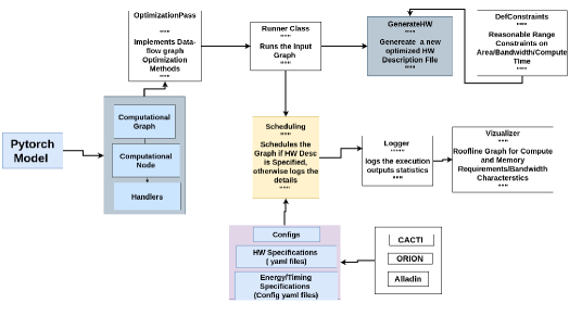
Figure 5: Software Class Diagram

References

- [1] Janibul Bashir, Khushal Sethi, and Smruti R Sarangi. Power efficient photonic network-on-chip for a scalable gpu. In Proceedings of the 13th IEEE/ACM International Symposium on Networks-on-Chip, pages 1–2, 2019.
- [2] DA Conners and Wen-Mei W Hwu. Compiler-directed dynamic computation reuse: Rationale and initial results. In MICRO-32. Proceedings of the 32nd Annual ACM/IEEE International Symposium on Microarchitecture, pages 158–169. IEEE, 1999.
- [3] Ilya Issenin, Erik Brockmeyer, Miguel Miranda, and Nikil Dutt. Data reuse analysis technique for software-controlled memory hierarchies. In Proceedings Design, Automation and Test in Europe Conference and Exhibition, volume 1, pages 202–207. IEEE, 2004.
- [4] A Ji, W Jung, J Woo, K Sethi, SL Luc, and AP Chandrakasan. Reconfigurable cnn processor for compressed networks. In Research Abstracts, page 14, 2020.
- [5] Zexi Ji, Wanyeong Jung, Jongchan Woo, Khushal Sethi, Shih-Lien Lu, and Anantha P Chandrakasan. Compacc: Efficient hardware realization for processing compressed neural networks using accumulator arrays. In 2020 IEEE Asian Solid-State Circuits Conference (A-SSCC), pages 1–4. IEEE, 2020.
- [6] P Kollig and BM Al-Hashimi. Simultaneous scheduling, allocation and binding in high level synthesis. Electronics Letters, 33(18):1516–1518, 1997.
- [7] Yujun Lin, Mengtian Yang, and Song Han. Naas: Neural accelerator architecture search. arXiv preprint arXiv:2105.13258, 2021.
- [8] Gabriel Marin and John Mellor-Crummey. Pinpointing and exploiting opportunities for enhancing data reuse. In ISPASS 2008-IEEE International Symposium on Performance Analysis of Systems and software, pages 115–126. IEEE, 2008.
- [9] Linyan Mei, Pouya Houshmand, Vikram Jain, Juan Sebastian P. Giraldo, and Marian Verhelst. Zigzag: A memory-centric rapid DNN accelerator design space exploration framework. CoRR, abs/2007.11360, 2020.
- [10] Angshuman Parashar, Priyanka Raina, Yakun Sophia Shao, Yu-Hsin Chen, Victor A Ying, Anurag Mukkara, Rangharajan Venkatesan, Brucek Khailany, Stephen W Keckler, and Joel Emer. Timeloop: A systematic approach to dnn accelerator evaluation. In 2019 IEEE international symposium on performance analysis of systems and software (ISPASS), pages 304–315. IEEE, 2019.
- [11] Ananda Samajdar, Yuhao Zhu, Paul Whatmough, Matthew Mattina, and Tushar Krishna. Scale-sim: Systolic cnn accelerator simulator. arXiv preprint arXiv:1811.02883, 2018.
- [12] Khushal Sethi. Design space exploration of algorithmic multi-port memories in high-performance application-specific accelerators. arXiv preprint arXiv:2007.09363, 2020.
- [13] Khushal Sethi. Efficient on-chip communication for parallel graph-analytics on spatial architectures. arXiv preprint arXiv:2108.11521, 2021.
- [14] Khushal Sethi, Vivek Parmar, and Manan Suri. Low-power hardware-based deep-learning diagnostics support case study. In 2018 IEEE Biomedical Circuits and Systems Conference (BioCAS), pages 1–4. IEEE, 2018.
- [15] Khushal Sethi and Manan Suri. Optimized implementation of neuromorphic hats algorithm on fpga. In 2019 IEEE International Symposium on Circuits and Systems (ISCAS), pages 1–5. IEEE, 2019.
- [16] Khushal Sethi and Manan Suri. Nv-fogstore: Device-aware hybrid caching in fog computing environments. arXiv preprint arXiv:2010.10562, 2020.
- [17] Xuan Yang, Mingyu Gao, Qiaoyi Liu, Jeff Setter, Jing Pu, Ankita Nayak, Steven Bell, Kaidi Cao, Heonjae Ha, Priyanka Raina, et al. Interstellar: Using halide’s scheduling language to analyze dnn accelerators. In Proceedings of the Twenty-Fifth International Conference on Architectural Support for Programming Languages and Operating Systems, pages 369–383, 2020.