Percolation in a triangle on a square lattice

Abstract

Percolation on a plane is usually associated with clusters spanning two opposite sides of a rectangular system. Here we investigate three-leg clusters generated on a square lattice and spanning the three sides of equilateral triangles. If the position and orientation of the triangles relative to the lattice are uniformly randomized, one obtains an efficient method of determining the percolation threshold, on par with the most advanced Monte Carlo methods developed for the rectangular geometry. The universal crossing probability for three-leg clusters is geometry-independent, which opens a way for further improvements of the method.

I Introduction

With a simple, purely geometrical definition and complex behavior that includes a phase transition, percolation has become an important theoretical model in statistical physics. It has also applications in various areas of science, like conductivity in strongly heterogeneous solids [1, 2], fluid flow in porous media [3, 4], epidemics [5], and thermal conductivity of composites [6].

While some critical exponents and crossing probabilities in 2-dimensional systems [7, 8, 9, 10, 11], as well as percolation thresholds in several particular models [12, 13, 14] are known rigorously, many results in this field has been obtained with computer simulations. Over the years, advanced numercial methods have been developed, like the Leath method [15, 16, 17], hull-generating walks [18, 19], gradient percolation [20, 21, 22], toroidal wrapping [23, 24, 25], spanning clusters [26, 27], rescaled particles [28], frontier tracking [29], parallelized percolation on distributed machines [30], dynamic programming [31], and the transfer matrix method [32, 33]. These methods, in all their diversity, share one common feature: they are usually implemented with the assumption that the system has a square (rectangular, hypercubic) geometry. This choice is quite natural: it corresponds to the most elementary and efficient computer data structure: array. It also facilitates implementation of useful boundary conditions, including wrapping boundaries. Wrapping boundaries, in turn, enable one to study percolation on cylinders and tori, the shapes for which strong theoretical results have been derived and for which boundary effects are minimized, which results in a faster convergence rate to the thermodynamic limit [23].

The symmetry of a rectangle is closely related to the required connectedness of a cluster: in spanning percolation the two sides that are checked for spanning are geometrically equivalent, and so are the remaining two. One expects that this configuration will produce quicker convergence to the thermodynamic limit than, for instance, a trapezoid. If one uses square systems, it is possible to investigate clusters that span or wrap in both directions simultaneously [23]. But what about spanning in other number of directions than two or four, for example, three? It was recently argued that the probability, $p_{3}$ that, in the thermodynamic limit, there exists a three-leg cluster touching the three sides of a triangle at the percolation threshold has a universal value $1/2$ [34, 11]. This result is supposed to be valid for any lattice and even systems of arbitrary shape, in which case their perimeter must be divided into three disjoint parts (arcs). For self-matching lattices this property holds even for finite systems.

The aim of the paper is to investigate whether the property of $p_{3}\to 1/2$ can be used to develop an efficient method of finding the percolation threshold, $p_{\mathrm{c}}$, for planar lattices. To this end, we investigate the well-known case of the site percolation on a square lattice, assuming, however, that the system is in the shape of an equilateral triangle, the simplest geometry with the three-fold symmetry corresponding to the three legs of the clusters. The precise value of $p_{\mathrm{c}}$ in this model [33],

$$p_{\mathrm{c}}=0.592\,746\,050\,792\,10(2),$$ (1)

will be used as a reference value against which the method will be evaluated.

II Method

We start from placing an equilateral triangle with sides of length $L$ on a square lattice (Fig. 1).

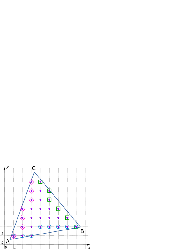
Figure 1: Geometry of the model. An equilateral triangle $ABC$ is located on a square lattice in such a way that its vertex $A$ is placed randomly inside $[0,1)\times[0,1)$ and the angle between side $AB$ and the direction of the $x$ axis is a random variable between 0 and 15 degrees. Circles, squares, and diamonds mark the ”edge” site corresponding to three sides of the triangle. A three-leg percolating cluster must contain at least one site from each of these groups.

Incompatibility of the symmetries of the triangle and the lattice gives rise to specific problems; for example, the number of lattice sites encompassed by a triangle is not invariant under translation and rotation, and the number of sites contained inside a triangle of side length $L$ only approximately scales as $L^{2}$, a problem particularly serious for small triangles. There are also problems of topological nature: if one side of the triangle is parallel to the $x$ axis, it cuts $\approx L$ lattice bonds, whereas the remaining two sides cut $\approx\sqrt{3}L$ bonds. Thus, the sides, even though of equal lengths, are not equivalent, which may have an adverse effect on the simulation convergence rate.

To mitigate these problems, for each $L$ we consider an ensemble of equilateral triangles randomly distributed and oriented relative to the underlying lattice. Symmetries of the lattice and the triangle allow to restrict the ensemble to the cases where vertex $A$ is distributed uniformly inside the square $[0,1)\times[]0,1)$, and the angle $\alpha$ made by side $AB$ and the direction of the $x$ axis is distributed uniformly between 0 and 15 degrees.

Each simulation starts from randomization of the location and orientation of the triangle. Then, a minimum bounding box for the triangle is computed such that its corners are at lattice sites. This will be the arena of the simulation: rectangular geometry trivializes the computation of the neighboring sites. Next, the set of the sites encompassed by the triangle is determined. We shall call them “active sites”. Only active sites can be occupied as the cluster grows. Some of these sites are marked as edge sites. We define three groups of edge sites, each corresponding to a triangle side. A site is an edge site to side $AB$ if a nearest-neighbor bond starting at this site cuts $AB$. Two other groups are defined similarly for sides $BC$ and $CA$. A site can be an edge site for more than one side (for example, the lattice sites nearest to vertices $A$ and $B$ in Fig. 1). We define a three-leg percolating cluster as a cluster that contains at least one site from each of these groups.

When the geometry has been established, a list of active sites is shuffled randomly (we used the 64-bit Mersenne twister mt19937 random number generator from the standard C++ library). During simulation proper, subsequent elements are popped from this list and the corresponding sites are marked as occupied. With each new site occupied, the union-find algorithm [23, 35] is used to monitor clusters’ growth. It also updates the information about the edge groups each cluster has reached. To this end, before the simulation begins, the union-find assigns to each site three bits that are used to signal the property of being connected to a given group of edge sites. This property is updated whenever clusters merge. A simulation ends when, for some cluster, all these bits are set to 1, which indicates that a three-leg percolating cluster has just been formed. Finally, the number of occupied sites is recorded.

In this way we obtained the distribution of the probability $R(n;L)$ that for the ensemble of a randomly positioned and oriented equilateral triangles of side $L$, with $n$ of their internal sites occupied, there is a three-leg cluster that spans all of its sides. We introduce the occupation probability

$$p=\frac{n}{S(L)},$$ (2)

where $S(L)=(\sqrt{3}/4)L^{2}$ is the expected number of lattice sites contained inside the triangle, which, due to the randomization of its placement and orientation, is equal to its area. Clearly, at percolation, $0<p<1$. Note, however, that in principle a triangle can hold more than $S(L)$ lattice sites within itself, leading to the possibility of $p>1$ when every or nearly every site is occupied. This, however, cannot happen at the onset of percolation; moreover, the upper bound for $p$ as $L\to\infty$ is 1, as it should.

An important quantity that we want to obtain from simulations is $R_{L}(p)$, the probability that, for site occupancy $p$, a triangle of side $L$ contains a cluster spanning all of its sides. While it is closely related to directly measured $R(n;L)$, the relation is, to some extent, unknown. First, we require $R_{L}(p)$ to be continuous, whereas $R(n;L)$ is discrete; second, $R(n;L)$ is not known exactly, but is estimated from simulations. The discrete nature of $R(n;L)$ is especially problematic for small $L$. For example, for $L=4$ only for 8 values of $n$ is this function different from 0 and 1. The usual way of dealing with these problems is to fit the data to some function (e.g. linear) in a vicinity of $p$. Here, however, we use the canonical ensemble method [23]. Its main idea is to weight the values of a discrete-value function $F$ with coefficients from the corresponding binomial distribution,

$$F(p)=\sum_{n=0}^{N}{N\choose n}p^{n}(1-p)^{N-n}F(n),$$ (3)

where $N$ is the number of sites in the system. This, however, poses a subtle problem: our simulations are performed for en ensemble of triangles in which $N$ may take on many values for fixed $L$, and its mean value, $S(L)$, is non-integer. We solve this by replacing the binomial distribution with its normal approximation, $\mathcal{N}\left(S(L)p,S(L)p(1-p)\right)$. This leads to

$$R_{L}(p)=\frac{1}{\sigma\sqrt{2\pi}}\sum_{n=0}^{\lfloor S(L)\rfloor}\exp\left({\frac{-(n-\mu)^{2}}{2\sigma^{2}}}\right)R(n;L),$$ (4)

with $\mu=S(L)p$, and $\sigma^{2}=S(L)p(1-p)$.

It is expected [34] that $R_{L}(p_{\mathrm{c}})\to 1/2$ as $L\to\infty$ (Fig. 2).

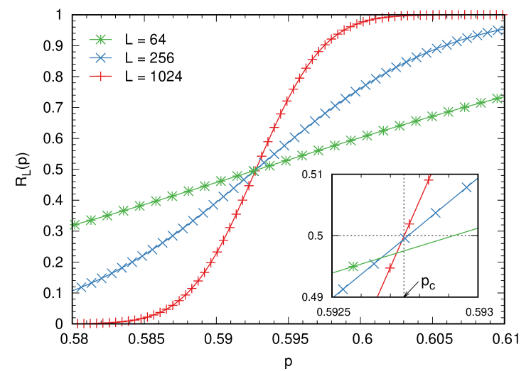
Figure 2: The probability $R_{L}(p)$ that a triangle of side $L$ with occupation probability $p$ of its internal sites contains a three-leg percolating cluster. Inset: close-up of the intersection region.

We can use this property to define an $L$-dependent approximation of the percolation threshold, $p^{*}_{L}$, defined as the solution to

$$R_{L}(p^{*}_{L})=1/2.$$ (5)

It was suggested [27] that $p^{*}_{L}$ can be approximated with

$$p^{*}_{L}\approx p_{\mathrm{c}}+L^{-1/\nu}\sum_{k=0}^{M}A_{k}L^{-k},$$ (6)

where $\nu=4/3$ is a critical exponent [7], $A_{k}$ are some nonuniversal parameters, and $M$ is a cut-off. However, in our case the sites forming ”edge groups” are situated inside the triangle, so the effective side length may differ from $L$. We therefore introduce another parameter, $\lambda$, that accounts for this uncertainty and helps to correct for the truncation of higher-order terms [36, 26],

$$p^{*}_{L}\approx p_{\mathrm{c}}+(L+\lambda)^{-1/\nu}\sum_{k=0}^{M}A_{k}(L+\lambda)^{-k},\quad L\geq L_{\mathrm{min}}.$$ (7)

where $L_{\mathrm{min}}$ is the cut-off for the system size below which this approximation is invalid.

The uncertainties of $p^{*}_{L}$ are estimated using the bootstrap method [37]. Next, the Levenberg–Marquardt algorithm for nonlinear least squares curve-fitting is applied to estimate the values of $p_{\mathrm{c}}$, $\lambda$, and $A_{k}$ in Eq. (7). The cut-offs $L_{\mathrm{min}}$ and $M$ are determined from the requirement that they should minimize the error estimate for $p_{\mathrm{c}}$. Quality of the fit was monitored with the regression standard error $s=\sqrt{\chi^{2}/\mathrm{dof}}$ (the square root of the chi-squared statistic per degree of freedom). For a good fit, $s$ is close to or smaller than 1.

III Results

We performed simulations of nearest-neighbor site percolation on a square lattice for triangles of side $L$ ranging from 4 to 1440 (all lengths in lattice units). The total number of active sites inside the triangles was $\approx 2\cdot 10^{14}$ for each $L\geq 16$, and between $10^{12}$ and $10^{13}$ for each $L<16$. The uncertainties of $p^{*}_{L}$ were below $3\cdot 10^{-7}$ for $L\geq 16$ and below $10^{-6}$ for $L<16$.

The first question we investigated was the convergence rate in Eq. (7). Since $R_{L}(p_{\mathrm{c}})\to 1/2$ as $L\to\infty$, and we use this limiting value in Eq. (5), $p^{*}_{L}-p_{\mathrm{c}}$ is expected to scale as $L^{-1-1/\nu}$ [26, 27], which is equivalent to $A_{0}=0$ in (7). When we set $M=1$ in (7) and used the best known value of $p_{\mathrm{c}}$, Eq. (1), we obtained $A_{0}=3.5\cdot 10^{-6}\pm 2\cdot 10^{-6}$ with the regression standard error $s\approx 0.6$, in agreement with the convergence rate $\sim L^{-1-1/\nu}$ = $L^{-7/4}$.

Setting $A_{0}=0$, we obtained $A_{1}=0.20707(6)$, $\lambda=0.9942(25)$, and

$$p_{\mathrm{c}}=0.592\,746\,10(4),$$ (8)

with $L_{\mathrm{min}}=16$ and the regression standard error $s\approx 0.7$. This fit is shown in Fig. 3.

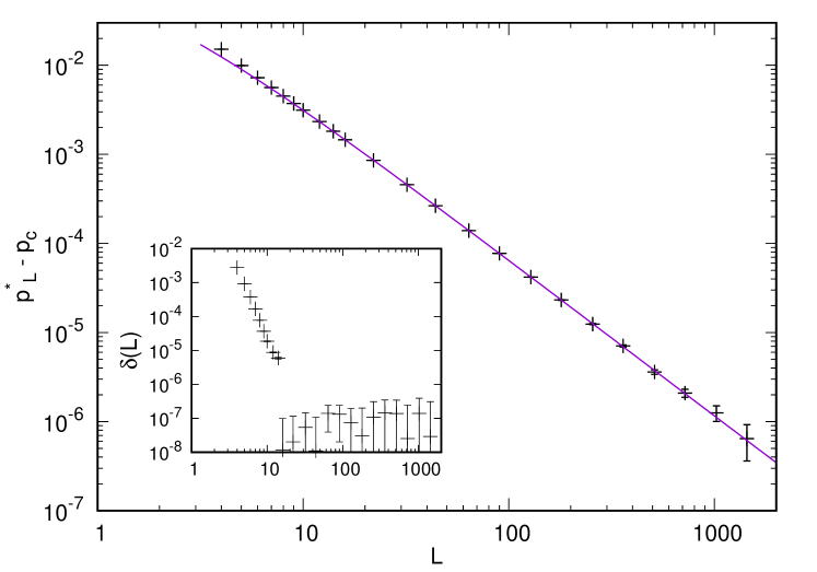
Figure 3: $p^{*}_{L}-p_{\mathrm{c}}$ (symbols) and its approximation $A_{0}/(L+\lambda)^{1+1/\nu}$ (line). Inset: $\delta(L)=|p^{*}_{L}-p_{\mathrm{c}}-A_{0}/(L+\lambda)^{1+1/\nu}|$, the error introduced by using (7) with $M=1$ and $L_{\mathrm{min}}=16$.

The value of $p_{\mathrm{c}}$ is in agreement with Eq. (1). In terms of measurement precision, our method turns out to be at least on par with alternative simulation methods based on Monte Carlo sampling ([32, 38] and references therein). The value of $s$ being less than 1 indicates that the fit is good: actually, the difference between $p^{*}_{L}$ and its approximation $p_{\mathrm{c}}+A_{1}/(L+\lambda)^{1+1/\nu}$ is less than $2\cdot 10^{-7}$ for all $L\geq 16$ (Fig. 3, inset). For $4\leq L<16$ it behaves roughly as $L^{-\omega}$ with $\omega=6.0(4)$. This suggests that $A_{2},A_{3},A_{4}\approx 0$ in (7). However, fits in this region are poor and the hypothesis that three consecutive terms in (7) vanish should be taken with caution.

The role of $\lambda$ in (7) is to help reduce both $M$ and $L_{\mathrm{min}}$. One could do without it and set $\lambda=0$, effectively reducing (7) to (6). This would require taking $M=3$, with the total of 4 fitting parameters instead of 3. The uncertainty of $p_{\mathrm{c}}$ thus obtained would be higher by about 25% compared to the value reported in (8), which is acceptable, but the uncertainty of $A_{1}$ would be tripled.

Is randomization of the position and orientation of triangles necessary? When we fixed vertex $A$ at (x, y) and $B$ at (x + L, y) with $x=y=0.5$, we found that the left hand side of (7) still exhibits the $\sim L^{-1-1/\nu}$ behavior, but it also contains a significant contribution of what can be regarded as noise (Fig. 4).

Figure 4: $p^{*}_{L}-p_{\mathrm{c}}$ for triangles with vertex $A$ fixed at $(0.5,0.5)$ and angle $\alpha=0$. The dashed line is a guide to the eye with the slope $-1-1/\nu=-1.75$.

Its magnitude is so large that it makes the method practically useless. When we set $x=0.5$ and treated $y$ as a random variable uniformly distributed in $(0,1)$, this “noise” was still present, though its magnitude was much smaller (data not shown). Thus, full randomization ot triangles’ position and orientation appears necessary for lattice-based systems. However, for continuous systems (e.g. percolation of overlapping discs or squares [39]) this step can be omitted.

Using the canonical ensemble method to estimate $R_{L}(p)$ is crucial, because it works well even for small system sizes, where the discrete nature of $R(n;L)$ is quite problematic for other methods, e.g. those based on approximation. Further studies are necessary to check whether applying the exact canonical weighting could improve the validity of Eq. (7) for small $L$.

The simulations were run in parallel on several computers with varying computational power. Simulations depicted in Fig. 3 would have taken about 1.5 years if done only on the PC on which this paper was written (a four-core processor running 8 threads in parallel at 3.4 GHz). The computational overhead introduced by randomization of the triangle orientation is about 100% for very small systems ($L=4$), but quickly drops to $\approx 10\%$ for $L\gtrsim 50$. The highest (multi-threaded) computational efficiency is obtained for $L\approx 64$, for which one occupied site is processed at $\approx 33$ processor clock cycles. It decreases $\approx 5$ times for the smallest and largest system sizes considered here, the former due to the randomization overhead, the latter due to processor cache misses.

IV Discussion

The method presented here can be applied to other system shapes (with an arbitrary division of their boundary into three compact regions), lattices, and cluster connectedness definitions, all with the universal three-leg crossing probability $1/2$. In contrast to this, universal spanning (”two-leg”) and wrapping probabilities are known only for some particular system shapes, e.g. rectangles, and for more complicated cases would have to be treated as an additional unknown. A disadvantage of our method is a rather slow convergence rate to the thermodynamic limit, most likely related to open boundary conditions [40].

The method can be generalized to more complex shapes, e.g., convex polygons. The bounding box can be determined from the maximum and minimum values of the vertex coordinates. Then one can iterate over each of the sites lying inside the bounding box and test if it lies inside the polygon and if so, if it is adjacent to any of the polygon’s sides. This general method can be used for complex networks, e.g., Penrose tiling [41]. A more efficient way is to shoot a small number of “rays“ in such a way that they cut all internal sites of the polygon. In the case depicted in Fig. 1 they could be shot vertically or horizontally along the grid lines. If a ray hits a convex polygon, it enters the system at some point $q_{1}$ and leaves it at some $q_{2}$ ($q_{1}$ and $q_{2}$ can coincide). Any lattice site between $q_{1}$ and $q_{2}$ must be an internal site and all edge sites must lie in their close proximity. This reduces the computational complexity of discovering the edge sites from quadratic to linear in the characteristic system size. This method should be applicable for all networks based on regular lattices, including networks with voids and bottlenecks [42] and frustrated lattices [43]. Once the geometry of the system has been established, the remaining steps are essentially the same as in traditional methods.

The angle by which each system is rotated can be arbitrary. Here we reduced it to the range from 0 o 15 degrees only because for equilateral triangles some code simplifications are then possible. For example, no sites adjacent to edge $AB$ in Fig. 1 can have the same vertical coordinates.

Bond percolation can be treated in a very similar way. Rather than with active sites, one would deal with active bonds defined as those with at least one end lying inside the system. Edge bonds would be then defined as those that cut a given system edge.

Monte Carlo methods, including the one presented here, for simple planar lattice models have recently become overshadowed by transfer-matrix methods [33]. Still, we hope that our work can prove useful in more complicated cases, like networks with voids and bottlenecks, continuous models, or in higher-dimensions [44].

V Conclusions

We have shown that Monte-Carlo simulations in systems with incompatible symmetries of their geometry and the underlying lattice can be efficient in determining the percolation threshold. The key step is randomization of the system orientation and position relative to the lattice. The computational overhead related to this additional step is acceptable. Although the convergence rate to the thermodynamic limit is slower than in some methods based on wrapping, this is compensated by very small (or perhaps even vanishing) values of several higher-order terms and the possibility of using small lattices.

Three-leg clusters have proved useful in determining the value of the percolation threshold. Their advantage is that the universal crossing probability associated with them is geometry-independent, which opens the room for further improvements of the method.

References

- Hunt [2001] A. Hunt, Applications of percolation theory to porous media with distributed local conductances, Advances in Water Resources 24, 279 (2001).
- Bessaguet et al. [2019] C. Bessaguet, E. Dantras, G. Michon, M. Chevalier, L. Laffont, and C. Lacabanne, Electrical behavior of a graphene/PEKK and carbon black/PEKK nanocomposites in the vicinity of the percolation threshold, Journal of Non-Crystalline Solids 512, 1 (2019).
- Sahimi [1993] M. Sahimi, Flow phenomena in rocks: from continuum models to fractals, percolation, cellular automata, and simulated annealing, Rev. Mod. Phys. 65, 1393 (1993).
- Bolandtaba and Skauge [2011] S. Bolandtaba and A. Skauge, Network modeling of EOR processes: a combined invasion percolation and dynamic model for mobilization of trapped oil, Transport in porous media 89, 357 (2011).
- Ziff [2021] R. M. Ziff, Percolation and the pandemic, Physica A: Statistical Mechanics and its Applications 568, 125723 (2021).
- Shtein et al. [2015] M. Shtein, R. Nadiv, M. Buzaglo, K. Kahil, and O. Regev, Thermally conductive graphene-polymer composites: size, percolation, and synergy effects, Chemistry of Materials 27, 2100 (2015).
- Stauffer and Aharony [1994] D. Stauffer and A. Aharony, Introduction to Percolation Theory, 2nd ed. (Taylor and Francis, London, 1994).
- Cardy [1992] J. L. Cardy, Critical percolation in finite geometries, Journal of Physics A: Mathematical and General 25, L201 (1992).
- Lawler et al. [2002] G. Lawler, O. Schramm, and W. Werner, One-arm exponent for critical 2D percolation, Electronic Journal of Probability 7, 1 (2002).
- Smirnov [2001] S. Smirnov, Critical percolation in the plane: conformal invariance, cardy’s formula, scaling limits, Comptes Rendus de l’Académie des Sciences - Series I - Mathematics 333, 239 (2001).
- Flores et al. [2017] S. M. Flores, J. J. H. Simmons, P. Kleban, and R. M. Ziff, A formula for crossing probabilities of critical systems inside polygons, Journal of Physics A: Mathematical and Theoretical 50, 064005 (2017).
- Sykes and Essam [1964] M. F. Sykes and J. W. Essam, Exact critical percolation probabilities for site and bond problems in two dimensions, Journal of Mathematical Physics 5, 1117 (1964), https://doi.org/10.1063/1.1704215 .
- Kesten [1980] H. Kesten, The critical probability of bond percolation on the square lattice equals 1/2, Communications in Mathematical Physics 74, 41 (1980).
- Wierman [2009] J. C. Wierman, Percolation thresholds, exact, in Encyclopedia of Complexity and Systems Science, edited by R. A. Meyers (Springer New York, New York, NY, 2009) pp. 6579–6587.
- Leath [1976] P. L. Leath, Cluster size and boundary distribution near percolation threshold, Phys. Rev. B 14, 5046 (1976).
- Lorenz and Ziff [1998] C. D. Lorenz and R. M. Ziff, Precise determination of the bond percolation thresholds and finite-size scaling corrections for the sc, fcc, and bcc lattices, Phys. Rev. E 57, 230 (1998).
- Xun et al. [2021] Z. Xun, D. Hao, and R. M. Ziff, Site percolation on square and simple cubic lattices with extended neighborhoods and their continuum limit, Phys. Rev. E 103, 022126 (2021).
- Voss [1984] R. F. Voss, The fractal dimension of percolation cluster hulls, Journal of Physics A: Mathematical and General 17, L373 (1984).
- Ziff et al. [1984] R. M. Ziff, P. T. Cummings, and G. Stells, Generation of percolation cluster perimeters by a random walk, Journal of Physics A: Mathematical and General 17, 3009 (1984).
- Rosso et al. [1985] M. Rosso, J. F. Gouyet, and B. Sapoval, Determination of percolation probability from the use of a concentration gradient, Phys. Rev. B 32, 6053 (1985).
- Ziff and Sapoval [1986] R. M. Ziff and B. Sapoval, The efficient determination of the percolation threshold by a frontier-generating walk in a gradient, Journal of Physics A: Mathematical and General 19, L1169 (1986).
- Tencer and Forsberg [2021] J. Tencer and K. M. Forsberg, Postprocessing techniques for gradient percolation predictions on the square lattice, Phys. Rev. E 103, 012115 (2021).
- Newman and Ziff [2001] M. E. J. Newman and R. M. Ziff, Fast Monte Carlo algorithm for site or bond percolation, Phys. Rev. E 64, 016706 (2001).
- Wang et al. [2013] J. Wang, Z. Zhou, W. Zhang, T. M. Garoni, and Y. Deng, Bond and site percolation in three dimensions, Phys. Rev. E 87, 052107 (2013).
- Koza and Poła [2016] Z. Koza and J. Poła, From discrete to continuous percolation in dimensions 3 to 7, Journal of Statistical Mechanics: Theory and Experiment 2016, 103206 (2016).
- Ziff [1992] R. M. Ziff, Spanning probability in 2D percolation, Phys. Rev. Lett. 69, 2670 (1992).
- de Oliveira et al. [2003] P. M. C. de Oliveira, R. A. Nórbrega, and D. Stauffer, Corrections to finite size scaling in percolation, Brazilian Journal of Physics 33, 616 (2003).
- Torquato and Jiao [2012] S. Torquato and Y. Jiao, Effect of dimensionality on the continuum percolation of overlapping hyperspheres and hypercubes. II. Simulation results and analyses, The Journal of Chemical Physics 137, 074106 (2012).
- Quintanilla et al. [2000] J. Quintanilla, S. Torquato, and R. M. Ziff, Efficient measurement of the percolation threshold for fully penetrable discs, Journal of Physics A: Mathematical and General 33, L399 (2000).
- Pruessner and Moloney [2003] G. Pruessner and N. R. Moloney, Numerical results for crossing, spanning and wrapping in two-dimensional percolation, Journal of Physics A: Mathematical and General 36, 11213 (2003).
- Yang et al. [2013] Y. Yang, S. Zhou, and Y. Li, Square++: Making a connection game win-lose complementary and playing-fair, Entertainment Computing 4, 105 (2013).
- Feng et al. [2008] X. Feng, Y. Deng, and H. W. J. Blöte, Percolation transitions in two dimensions, Phys. Rev. E 78, 031136 (2008).
- Jacobsen [2015] J. L. Jacobsen, Critical points of Potts and O(N) models from eigenvalue identities in periodic Temperley-Lieb algebras, Journal of Physics A: Mathematical and Theoretical 48, 454003 (2015).
- Koza [2019] Z. Koza, Critical in percolation on semi-infinite strips, Phys. Rev. E 100, 042115 (2019).
- Cormen et al. [2009] T. H. Cormen, C. E. Leiserson, R. L. Rivest, and C. Stein, Introduction to algorithms (MIT press, 2009).
- Levinshteln and Efros [1975] M. Levinshteln and L. Efros, The relation between the critical exponents of percolation theory, Zh. Eksp. Teor. Fiz 69, 396 (1975).
- Press et al. [2007] W. H. Press, S. A. Teukolsky, W. T. Vetterling, and B. P. Flannery, Numerical Recipes 3rd Edition: The Art of Scientific Computing, 3rd ed. (Cambridge University Press, USA, 2007).
- Lee [2008] M. J. Lee, Pseudo-random-number generators and the square site percolation threshold, Phys. Rev. E 78, 031131 (2008).
- Mertens and Moore [2012] S. Mertens and C. Moore, Continuum percolation thresholds in two dimensions, Phys. Rev. E 86, 061109 (2012).
- Hovi and Aharony [1996] J.-P. Hovi and A. Aharony, Scaling and universality in the spanning probability for percolation, Phys. Rev. E 53, 235 (1996).
- Yonezawa et al. [1989] F. Yonezawa, S. Sakamoto, and M. Hori, Percolation in two-dimensional lattices. I. A technique for the estimation of thresholds, Phys. Rev. B 40, 636 (1989).
- Haji-Akbari and Ziff [2009] A. Haji-Akbari and R. M. Ziff, Percolation in networks with voids and bottlenecks, Phys. Rev. E 79, 021118 (2009).
- Haji-Akbari et al. [2015] A. Haji-Akbari, N. Haji-Akbari, and R. M. Ziff, Dimer covering and percolation frustration, Phys. Rev. E 92, 032134 (2015).
- Gori and Trombettoni [2015] G. Gori and A. Trombettoni, Conformal invariance in three dimensional percolation, Journal of Statistical Mechanics: Theory and Experiment 2015, P07014 (2015).