Explicit caching HYB: a new high-performance SpMV framework on GPGPU

Abstract.

Sparse Matrix-Vector Multiplication (SpMV) is a critical operation for the iterative solver of Finite Element Methods on computer simulation. Since the SpMV operation is a memory-bound algorithm, the efficiency of data movements heavily influenced the performance of the SpMV on GPU. In recent years, many research is conducted in accelerating the performance of SpMV on the graphic processing units (GPU). The performance optimization methods used in existing studies focus on the following areas: improve the load balancing between GPU processors, and reduce the execution divergence between GPU threads. Although some studies have made preliminary optimization on the input vector fetching, the effect of explicitly caching the input vector on GPU base SpMV has not been studied in depth yet.In this study, we are trying to minimize the data movements cost for GPU based SpMV using a new framework named” explicit caching Hybrid (EHYB)”. The EHYB framework achieved significant performance improvement by using the following methods:

1. Improve the speed of data movements by partitioning and explicitly caching the input vector to the shared memory of the CUDA kernel.

2. Reduce the volume of data movements by storing the major part of the column index with a compact format.

We tested our implementation with sparse matrices derived from FEM applications in different areas. The experiment results show that our implementation can overperform the state-of-the-arts implementation with significant speedup, and leads to higher FLOPs than the theoryperformance up-boundary of the existing GPU-based SpMV implementations.

1. Introduction

Sparse Matrix-Vector Multiplication (SpMV) evaluates the results of $y=A\times x$, where $A$ is a sparse matrix and $x$ and $y$ are (usually) dense vectors. SpMV is a critical operation for a wide range of scientific computing applications, especially in the iterative solver for the very large sparse linear system derived from the partial differential equation (PDE) in Finite Element Methods (FEM). With the computing capability for single-core processors limited by the power consumption problem that came with increasing frequency scaling (Mittal and Vetter, 2015), using the massive parallel computing processor such as general-purpose graphic processing units (GPGPU) became a must to improve the performance of scientific computing applications. For the important role of SpMV in scientific computing, the efficient parallel implementation of SpMV on the GPGPU architectures has been a hot research topic in the field of high-performance computing(Anzt et al., 2020a). And some of the new developed algorithms was integrated into the CUSPARSE library provided by NVIDIA.

In this study, we are work on developing a GPGPU based SpMV implementation leads to better performance than the state-of-art implementation of SpMV on GPU with reasonable preprocessing time. We try to optimizing the SpMV using the following methods:

• Reduce the amount of data movements by reduce the I/O volume for SpMV and

• Approaching the high efficiency of data movements by partitioning and explicitly caching the input vector to the shared-memory of GPU device.

The above methods are accomplished through a ”partitioning, reordering, and caching” procedure, categorized as preprocessing of the sparse matrix. The time cost of preprocessing procedure is comparable to the time cost for the format change of the sparse matrix, and the partitioning/reordering will introduce an extra preprocessing time. And the preprocessing time costs, based on or experiment, around 400$\times$ to 2000$\times$ of a single SpMV on GPU.

We tested our implementation with large sparse matrices derived from FEM on structure, biomedical, Computational Fluid Dynamic (CFD), and electromagnetics problems. Most of these matrices are generated with an unstructured mesh (which leads to an irregular sparse pattern). Based on our experiment on the Tesla V100 GPU, the optimized SpMV kernel we developed can leads to better performance when compared to the state-of-the-art GPU based library functions on SpMV.

2. Background

2.1. Concepts related to GPU code optimization

Implementing SpMV in GPGPU efficiently requires the code to be optimized according to the GPGPU architecture. Since the CUDA programming model becomes the de facto for GPGPU parallel programming, all the architecture-related code optimization discussed in this study will be based on the NVIDIA GPGPU and CUDA program model.

In the CUDA programming model, the GPU code is offloaded to the devices through kernel function and all the kernel functions executed the instructions which will be executed with a block of threads. The block will be divided into warps, which is a group of 32 threads. The GPU stream multiprocessor (SM) will try to execute the instructions belongs to one warp at each clock cycle. It is common that multiple warps of the same block were dispatched to one SM, and the pipeline of that SM will switch between the contexts of warps when the current warp is stall (i.e. waiting for data). Threads within the same warp execute different instructions will cause thread divergence. When thread divergence happened, the instructions from multiple threads will be executed serially.

GPU memory hierarchy is different compared to CPU memory hierarchy. According to the terminologies of CUDA, GPU memory space can be briefly categorized as: shared memory L1/texture cache, register file, L2 cache and global memory. Register files are the memory space used for stack variables of the CUDA threads. Global memory usually represents the RAM which is installed outside the GPU chip. The global memory is connected to the GPU chip wich DDR/HBM memory interface with limited bandwidth (which is 900 GB/s for Tesla V100 used in this study) and the latency of global memory can be hundreds of clock cycles of GPU chip. The L1/texture cache and shared memories are ”fast memory” which is consider as a part of the SM, these memory are connected to the SM processing units with a verh high bandwidth connections.

maximize the hit rate of the input vector fetch of SpMV operations.

2.2. Related research about SpMV on GPU

Significant research about optimizing the SpMV performance on GPGPU is conducted because SpMV is important in a large range of computing applications. This research starts at (Bell and Garland, 2009), where the researchers start to propose different sparse matrix storage formats to reduce the imbalance of GPU programming on matrices with different nonzero patterns. The format for high-performance SpMV on GPU examined by (Bell and Garland, 2009) includes Ellpack(ELL), Compressed Row(CSR), Coordinate(COO), Diagonal(DIA), and Hybrid(HYB). Numerous of research is conducting on finding the best format automatically for different blocks, and optimal partitioning the matrix according to the nonzero patterns using statistical methods(Li et al., 2014)(Yang et al., 2017)(Yang et al., 2018), or machine learning methods(Dufrechou et al., 2021)(Nisa et al., 2018)(Benatia et al., 2016). There are also research focus on developing new formats which may leads to better balancing on a wide range of matrices, the proposed novel format includes SELLp(Anzt et al., 2014), BiELL(Zheng et al., 2014), and JAD(Cevahir et al., 2009), to name a few. Among these novel formats, the best performance format is the BCOO format proposed by the yaspmv framework(Yan et al., 2014), however, the BCOO format requires an extremely long time of preprocessing (averagely 155,000$\times$)

In recent year, new algorithms are developed for efficiently conducting GPU based SpMV for imbalanced matrices with CSR format. Such as CSR5(Liu and Vinter, 2015), merge-based SpMV(Merrill and Garland, 2016), and hola SpMV(Steinberger et al., 2017). These new algorithms can provides excellent performance in a variety of nonzero patterns without format conversion. In the latest NVIDIA CUSPARSE library, a generic interface for SpMV is introduced. According to (Anzt et al., 2020b), the generic interface SpMV kernel in CUSPARSE can overperform many GPU libraries without conversion.

However, research on improving the input vector fetch efficiency on GPU-based SpMV is limited. In this study, we proposed a new SpMV framework on GPU named Explicitly Caching Hybrid framework (EHYB), multiple optimization methods is applied to make this framework overperform the state-of-the-art SpMV functions on GPUs.

3. The framework of EHYB on GPU

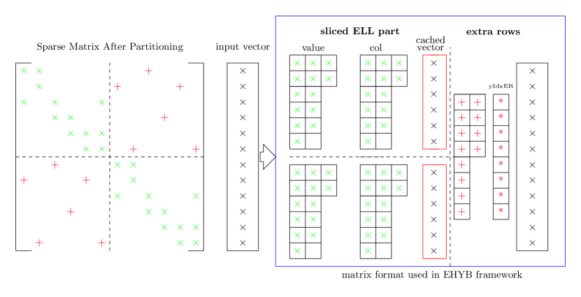
Figure 1. A sparse matrix in EHYB framework

Format description of EHYB

3.1. Graph-based partitioning as the first step of preprocessing

Figure 1 demonstrated the basic concepts of the EHYB framework. The first phase of the EHYB framework is to apply the graph-based partitioning to the input sparse matrix. Before partitioning, the sparse matrix will be recognized as an undirected graph with each row/column as a vertex and each entry as an edge connected the two vertexes related to its coordinate. After partitioning, the entries of the sparse matrix will be assigned to certain partitions, and their row index and column index as vertexes are most likely belong to the same partition. The left part of the figure 1 represents a sparse matric after the graph-based partitioning is applied. The SpMV operations on the major part of the entries in that matrix will only require input vector data with the index belongs to its partition (which was demonstrated as green $\times$ in the sparse matrix in figure 1). However, the partitioning can’t be perfect, which means there are still a few entries do not fall within this category, and these entries is demonstrated as $+$ in the figure. For these entries, the SpMV operations will require the input vector value with its index out of the partition of that entry.

For the entries represent as green $\times$ in figure 1, we can explicitly cache the input vector related to these entries in the shared memory of GPU. After the data is explicitly cached, the SpMV operations on the major part of the sparse matrix entries will not fetching data from the device memory of GPU. Instead of that, they will directly got the input vector value from the shared memory of GPU with much less latency.

Please be aware that the hypergraph-based partitioning is not suitable for the scenarios in this study. The hypergraph-based partitioning is developed for the SpMV operations running on a distributed memory system. For that scenario, the computing node only needs to fetching the same input vector value from other nodes once, because it can reuse the fetched data at the local memory. This premise is no longer valid in GPU architecture, which can be categorized as a shared memory system with an independent cache for each stream processor. In GPU, the input vector value fetched from other partitions will not stay in the cache for a long term. For that reason, the graph-based partitioning algorithm is more suitable for the EHYB framework in this paper.

3.2. The hybrid format of sparse matrix

To further improve the performance of the CUDA kernel function. The EHYB framework will store the sparse matrices to the format demonstrated as the left part of figure 1. From this figure we can find out that, the sparse matrix is split into two parts. The sliced ELL part stores the entries which only require input vector value from the cache, and the stride of the slice will be equal to the size of warp in GPU (which is 32). The post-partitioning reordering is conducted in a way that the reordered matrix will have its number of entries in row arranged in descending order within certain partitions. This reordering will reduce the thread divergence of CUDA warps since each thread belong to a warp will execute equal number of iterations on each slice of the matrix. The entries belong to the same partition will be processed by a single CUDA block because they need to share the input vector stored in the same cache.

The extra rows (ER) part of the EHYB matrix in figure 1 is also stored in an order according to its number of entries in the row. However, the input vector in the ER part of the matrix will not be cached into the shared memory. Also, an array of index yIdxER should be introduced for the ER part of the matrix, because the re-arrangement of the data is not a reordering, so we need an array to map the address of the ER data line to the real row number of the matrix.

The details about the implementation of preprocessing and CUDA kernels of EHYB will be demonstrated in the next section of this paper.

3.3. Input vector cache size

The number of partition and size of the input vector cache of EHYB framework can be determined using the following equation:

(1) $$K=MIN_{K\in\mathbb{Z}}(\frac{dimension\times\tau}{K\times P}<SHM^{max})$$

(2) $$VecSize=\frac{dimension}{K\times P}$$

Where $K$ is an integer value, $dimension$ is the number of rows in the matrix. $\tau$ is the number of bytes per value ($\tau=4$ for single precision) and $\tau=8$ for double precision). $P$ is the number of processor units of the GPU device. $P\times K$ is the number of partition of EHYB, and the input vector size can be calculated tough equation 2 The derivation of the equation 1 and 2 is straightforward, to maximize the performance of the SpMV kernel, we want to utilize all computing units (which is streaming processor in NVIDIA terminology) of the GPU. Also, we want to minimize the size of the ER entries of the EHYB matrix. So we set the vector cache size to the largest value which can make the number of partition equal to an integer which is multiple of the number of processing units in the GPU(which 80 SMX in the Tesla V100 GPU used in this study) .

3.4. reduce the memory footprint size of matrix

In figure 1, the col data of the sliced ELL part of the EHYB format stores the index of the input vector value the CUDA kernel will fetch during the SpMV operations. Consider index is used for fetching data from the cached vector in shared memory, and the vector cache size is limited by equation 1 and 2, we can confirm that the index value can’t be higher than $2^{16}$. This feature gives us the possibility to continue optimizing the EHYB framework by store the col data in figure 1 in short integer format. This will reduce the memory footprint of sliced ELL part by 25% in single precision, or 13.3% in double precision.

4. The implementation of EHYB

This section describes the detail of the implementation of preprocessing and CUDA kernel function of the EHYB framework. The ALgorithm 1 and 2 demonstrates the preprocessing phase of EHYB running on the host machine (CPU) and the CUDA kernel function described in algorithm 3 will be executed on the GPU.

4.1. Preprocessing and matrix reordering for the EHYB framework

1

2$G(V,E)$ $\leftarrow$ InputMatrix ;

3 PartVec $\leftarrow$ ParMETIS($G(V,E)$);

4 $Struct$ $S\{introwIdx;intentries;\}$;

5 for row from $1$ to Dimension do

6       for col from $1$ to $nnz$ at row do

7             S_array1[row].rowIdx=row ;

8             if PartVec $[\textnormal{{col}}]==$ PartVec $[\textnormal{{row}}]$ then

9                   S_array1[row ].entries$+=1$;

10                   if S_array1[row].rowIdx$==0$ then S_array1[row].rowIdx=row ;

11                  

12             else

13                   S_array2[].entries$+=1$;

14                   if S_array2[row].rowIdx$==0$ then S_array2[row].rowIdx=row ;

15                  

16             end if

17            

18       end for

19      

20 end for

21sort(S_array2) according to entries;

22for PartId from $1$ to patition do

23       sort(S_array1[PartId $\times vectorCacheSize$ to (PartId + 1)$\times vectorCacheSize$]);

24      

25 end for

26for row from $1$ to Dimension do

27       ReorderTable [S_arry1[row ].rowidx]$\leftarrow$row ;

28      

29 end for

30for row from $1$ to $ER\_rowNumber$ do

31       ArrangeTable[S_array2[row ].rowidx]$\leftarrow$row ;

32       yIdxER[row ]$\leftarrow$ReorderTable[S_array2[row ].rowidx]

33 end for

34Generate the PositionELL and PositionER vector similar to SELLp(Anzt et al., 2014);

Algorithm 1 Preprocessing algorithm of EHYB framework

Algorithm 1 of this paper demonstrated the preprocessing phase 1 of the EHYB framework. This algorithm will generate several ”metadata” vectors for the EHYB framework. The input of this algorithm is a sparse matrix with the coordinate (COO) format. In line 2 of algorithm 1, the sparse matrix is converted to a graph and passed to a function of multi-thread METIS library for the graph-based partitioning. The partitioning will generate a vector (PartVec) which indicates the partition assigned to each vertex of the graph.

Line 3 to line 14 of algorithm 1 created the struct array which stores the number of entries in each row for the sliced ELL part and ER part of the EHYB matrix. This array will be used as the input of sort operations in line 16 and line 18. Please notice that the for loop in line 17 is the main difference between the reordering in EHYB framework and the regular METIS-based reodering. In this for loop, the reorder permutation is determined by the descending order of the number of entries in row. Line 20 to line 27 of algorithm 1 will generating the meta vector for the metadata vector for the reodering and re-arrangement operations.

After the metadata vectors for the EHYB format matrix are generated, the reordering of the matrix will be completed through Algorithm 2. In line 4 to line 5 of algorithm 2, the post-partitioning reordering will be conducted as the value and col index of matrix moved to the sliced ELL part of the HYB matrix. And in line 10 to line 13 of the Algorithm 2, the re-arrangement will move the entries of the matrix to the ER part of the EHYB matrix.

1

2for $row$ from $1$ to Dimension do

3       $k1\leftarrow 0$;$k2\leftarrow 0$;;

4       for in  do

5             if PartVec $[col]$  then

                   $ELL\_idx\leftarrow\textnormal{{PositionELL}}[\textnormal{{ReorderTable}}[row]]$ $+\textnormal{{ReorderTable}}[row]\%warpSize+k1\times warpSize$; ColELL [$ELL\_idx$]$\leftarrow$ReorderTable $[col]$; ValELL [$ELL\_idx$]$\leftarrow$InputMatrix $[row][col]$; $k1+=1$

6             else

                   $ER\_idx\leftarrow\textnormal{{PositionER}}[\textnormal{{ArrangeTable}}[row]]$ $+\textnormal{{ArrangeTable}}[row]\%warpSize+k2\times warpSize$; ColER $[ER\_idx]\leftarrow$ReorderTable $[col]\;$; ValER $[ELL\_idx]\leftarrow$InputMatrix $[row][col]$; $k2+=1$

7             end if

8            

9       end for

10      

11 end for

Algorithm 2 Reordering phase of EHYB framework

4.2. Balancing optimization in CUDA kernel

The format we utilized in EHYB is similar to SELLp, which may cause unbalancing on the SpMV operations. To overcome this problem, we introduced balancing optimization in the CUDA kernel of EHYB, which is demonstrated in algorithm 3.

In line 6 to line 12 of the algorithm 3 the warp of a CUDA threads will processing the SpMV operations on a slice of entries. After the warp finished processing the current slice, line 14 to line 17 of algorithm 3 will assign a new slice belonging to the same partition to this warp. The kernel will processing the ER part of the EHYB matrix with same routine. The only difference is when processing ER part, the kernel will find the next slice globally, instead of finding the slice from same patition.

1

2

3$SliceIdStart\leftarrow blockIdx\times SlicePerBlock$;

4 $SliceIdEnd\leftarrow SliceIdStart+SlicePerBlock$;

5 $SliceId\leftarrow SliceIdStart+warpIdx$;

CachedVec $\leftarrow$ InputVector $[partBoundary[blockIdx]$ $\rightarrow partBoundary[blockIdx+1]]$; while $SliceId<SliceEndId$ do

6       $row\leftarrow warpLane+SliceId\times warpSize$; $Position\leftarrow\textnormal{{PositionELL}}[SliceId]$; $Width\leftarrow\textnormal{{WidthELL}}[SliceId]$; for $k$ from $1$ to $Width$ do

             $dataIdx\leftarrow Position+warpSize\times k+warpLane$; $y+=\textnormal{{ValELL}}[dataIdx]\times$ $\textnormal{{CachedVec}}[colELL[dataIdx]]$;

7       end for

8      OutputVector [row ]$\leftarrow y$; if $warpLane==0$ then

9             $SliceId\leftarrow$atomicAdd($SliceId$);

10       end if

11      shfl($SliceId$);

12 end while

13$SliceIdER\leftarrow atomicAdd(GlobalSilcedIdER)$; Repreat Line 5 to 18 on ER part of the matrix;

Algorithm 3 CUDA kernel function for EHYB framework

5. Evaluation

In this section, we tested our implementation with 94 large sparse matrices derived from problems related to real-world physical problem simulation in various applications. The data used in the experiments were not deliberately selected to fit the algorithms in this paper; rather, we did our best to make the matrices used in the experiments come from different domains. The matrices used includes the structural problem, Computational Fluid Dynamic problems, electromagnetics problems, biomedical problems, power system, VLSI/semiconductor device problem, semiconductor processes problem, model reduction problems, and optimization problem. We exclude the matrices derived from web/DNA connections since the main purpose of this paper is to develop a high-performance SpMV framework for iterative solvers of the very large sparse linear system derived from PDE-based problems. For the limitation of space We list the name of matrices and performance of the EHYB framework on these matrices in the table at the appendix section. The experiments in this section are conducted on the SDSC expanse cluster GPU nodes. The server is equipped with NVIDIA V100 SMX2 GPU, 374 GB DDR4 memory (running at 2,500 MHz) and a 20 core Intel Xeon Gold 6248 CPU. The GPU nodes we used contains 4 GPUs per node, but all the experiments in this study only used one GPU for the CUDA kernel function and at most 16 CPU cores for the preprocessing phase of EHYB.

To compare with the start-of-the-art performance of the GPU based SpMV, as described in section 2, we will compare the EHYB performance with the performance of holaspmv, yaspmv (single precision only), CSR5, merge-based SpMV and the latest CUSPARSE generic SpMV interface with ALG1 and ALG2. The results is demonstrated in the following sections.

5.1. single precision result

Figure 2 demonstrates the performance of EHYB in single precision, please be aware that the yaspmv didn’t generate correct results in some of the large matrices (also observed in (Steinberger et al., 2017)), and we changed all _shfl_ related function in holaSpMV to the synchronized function with the same name because the unsynchronize _shfl_ function is no longer supported on CUDA 10.2.

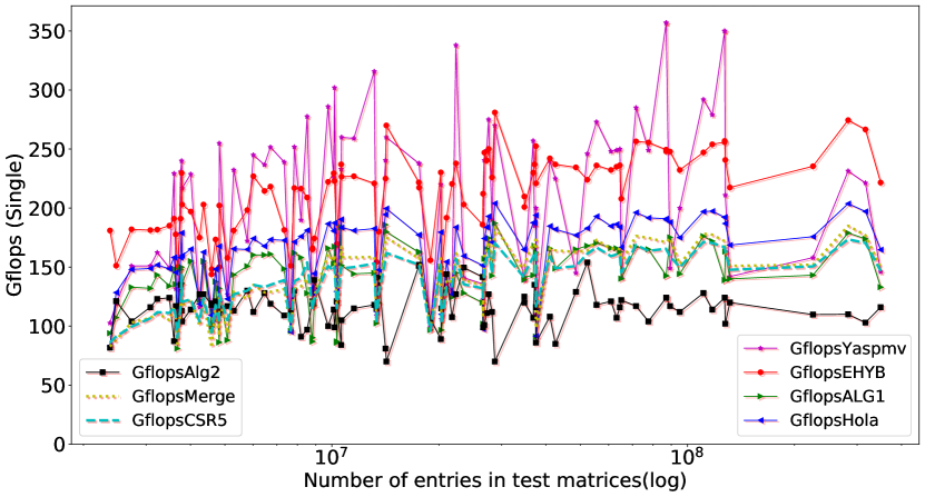
Figure 2. Float precision performance on 94 matrcies from suiteSparse

Gflop Line graphic for float precision

From figure 2 we can find out that EHYB over performs yaSpmv in most test data matrices (60%), the average speedup of EHYB versus yaSpmv is 1.15, and for larger matrices, EHYB performance gain comapred to yaSpmv is more significant. From table 1 we can also find out holaSpmv is the fastest framework which do not requires preprocessing. Averagely EHYB is 1.3$\times$ faster than holaSpmv in single precision.

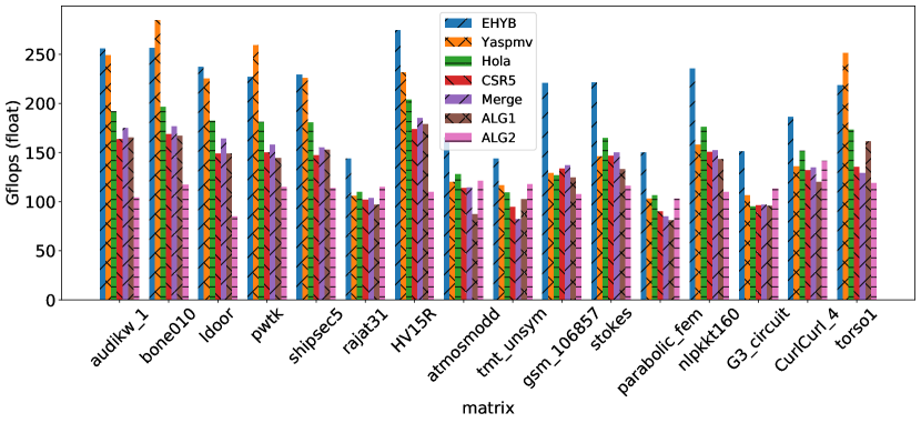
Figure 3. Single precision performance of 16 commonly tested matrices

float Gflop 16 matrices bar

SpMV framework:	EHYB is faster in % of matrices	max speedup	min speedup	average speedup
yasmpv	60.6%	2.0	0.69	1.13
holaspmv	100%	2.4	1.05	1.304
CSR5	100%	1.89	1.305	1.53
Merge	100%	2.25	1.31	1.517
ALG1	100%	2.42	1.21	1.518
ALG2	100%	4.0	1.21	1.90

Table 1. Speed up of EHYB versus other frameworks on single precision performance

5.2. double precision result

Figure 4 and figure 5 demonstrates the performance of EHYB compared with other implementations. The yaspmv library didn’t support double precision, so we compared the performance of EHYB with the remaining frameworks.

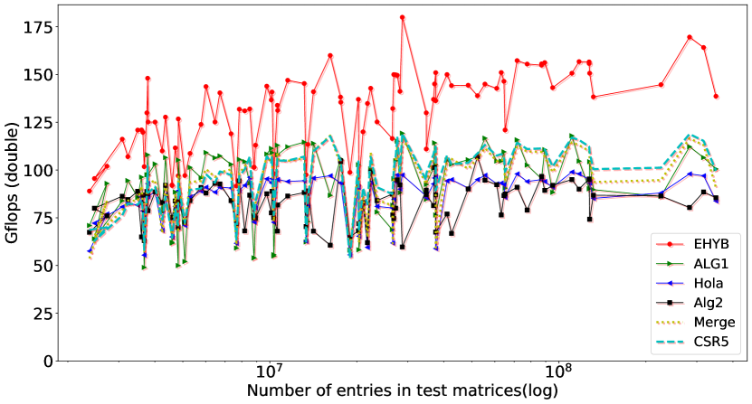
Figure 4. Double precision performance on 94 test matrices

Gflop Line graphic for double precision

From figure 4 we can find out the EHYB overperforms the other frameworks in all test matrices with a significant performance gain. The hola spmv performs solver than fastest CUSPARSE interface at most matrices in double precision tests, which is not match with the reuslts of single precision experiment. According to table 2, in double precision experiment, the CSR5 framework becomes the fastest framework besides EHYB.

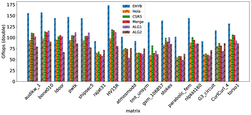
Figure 5. Double precision performance of 16 commonly tested matrices

double Gflop 16 matrices bar

SpMV framework:	max speedup	min speedup	average speedup
holaspmv	2.3	1.26	1.5
CSR5	1.84	1.13	1.38
Merge	2.29	1.15	1.41
ALG1	2.07	1.07	1.45
ALG2	3.01	1.19	1.59

Table 2. Speed up of EHYB versus other frameworks on double precision performance

6. preprocessing time cost and the significance of this study

Figure 6 demonstrates the preprocessing time of EHYB framework for 16 commonly tested sparse matrices. The preprocessing time cost can be decomposed into two parts: the partitioning part and the reordering part. In this study, we conducting the METIS partitioning with 16 threads on the host CPU (Intel Xeon Gold 6248). From figure 6 we can find out that the partitioning time cost for EHYB is around 400$\times$ to 1500$\times$ of the time cost of single SpMV operations on the GPU. And the reordering time cost is 50$\times$ to 400$\times$. The total preprocessing time will be around 500$\times$ to 2000$\times$. We should notice that the main part of the reordering time cost is caused by the sort operations in algorithm 1, currently, we conducting the sort operation with single thread, we expect that the reordering time will reduce significantly if the multi-thread sort algorithm is applied.

Although EHYB performs significant preprocessing, its preprocessing time cost is still around 100$\times$ less than the yaspmv(Yan et al., 2014) while it overperforms yaspmv on our experiments. The performance gain is also stable when compared to the time cost machine-learning-based partitiong/reordering preprocessing technology for GPU based SpMV (Dufrechou et al., 2021) (Benatia et al., 2016).

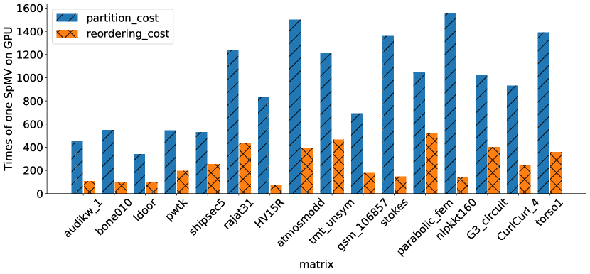
Figure 6. Preprocessing time for 16 commonly tested matrices

preprocessing bar fig

There are concerns about whether this research will benefit the real-world applications. The major reason for these concerns is: whether the SpMV operations still dominate the time cost of solving the linear system in the latest FEM algorithms. Since the modern preconditioned iterative solver has a high convergence rate, the solver can find the solution with less iterations, which makes it impossible to amortize the cost of preprocessing phase required by EHYB.

The widely cited classic literature (Saad, 2003) indicates that the time costs for SpMV dominated the overall time consumed for FEM-based simulation for large 3D problems. A recent book(Bertaccini and Durastante, 2018) also described this property of the FEM applications. On the other hand, in recent years, many new methods are developed on building high-efficient preconditioner for large linear systems derived from PDE. The algebraic multigrid (AMG) preconditioner(Boyle et al., 2010) can significantly improve the convergence rate of the iterative solver, thus reduce the iteration number to several hundred to several dozens(Isotton et al., 2021a). When AMG preconditioner is applied, building preconditioner matrices on coarser levels of a hierarchy of levels and forming and applying prolongation may cost more time than the the SpMV operations.

However, efficiently parallelize the AMG algorithm with the massive parallel accelerator such as GPGPU is a challange problem(Naumov et al., 2015). In GPGPU platform, the sparse approximate inverse (SPAI) preconditioner works well in many real-world applications according to latest literature(Isotton et al., 2021b)(Pearson and Pestana, 2020)(Singh and Ahuja, 2020). The high-performance SpMV kernel proposed in this paper will significantly improve the performance of the SPAI preconditioned iterative solver on GPGPU, since the SpMV operation will still be the most time consuming part of the iterative solver with SPAI preconditioner(Gao et al., 2021)(Georgescu et al., 2013).

The SPAI preconditioned iterative solver usually requires thousands of iterations to converge(Isotton et al., 2021b). Also, in transient simulation, the solver will repeatly solving the same linear system with hundreds of time steps(Kaehler and Henneberger, 2004). For transient simulation on real-world problems, the result of the preprocessing phase in EHYB is shared by hundreds of thousands of iterations. We can safely assume that the preprocessing time cost for EHYB can be amortized when applying the SPAI preconditioned solver for transient simulation problems.

7. Conclusion

In this study, we developed a novel SpMY framework on GPU named EHYB. The EHYB framework improves the speed of data movements by partitioning and explicitly caching the input vector to the shared memory of the CUDA kernel. The EHYB framework also reduces the volume of data movements by storing the major part of the column index in a compact format. The CUDA kernel function in EHYB is optimized to improving the balance between warps of CUDA threads. We tested the EHYB framework with a large number of sparse matrices derived from real-world applications. The experiment results indicate that the EHYB framework can overperform stat-of-the-art SpMV frameworks.

Appendix A Source code

The source code of this paper is available at: https://github.com/Chong-Chen-UNLV/EHYB_SPMV_GPU

Appendix B Matrices used for testing

Matrix name	Category	Dimension	Entries	Matrix name	Category	Dimension	Entries
poisson3D	CFD	85,623	2,374,949	ship_003	Structural	121,728	8,086,034
atmosmodj	CFD	1,270,432	8,814,880	BenElechi1	3D Problem	245,874	13,150,496
vas_stokes_1M	VLSI	1,090,664	34,767,207	Hook_1498	Structural	1,498,023	60,917,445
CurlCurl_1	Model Reduction	226,451	2,472,071	laminar_duct3D	CFD	67,173	3,833,077
CurlCurl2	Model Reduction	806,529	8,921,789	memchip	Circuit Simulation	2,707,524	14,810,202
inline1	Structural	503,712	36,816,342	Geo_1438	Structural	1,437,960	63,156,690
windtunnel_evap3d	CFD	40,816	2,730,600	cant	3D problem	62,451	4,007,383
m_t1	Structural	97,578	9,753,570	CurlCurl_3	Model Reduction	1,219,574	13,544,618
PFlow_742	3D problem	742,793	37,138,461	Serena	Structural	1,391,349	64,131,971
cfd2	CFD	123,440	3,087,898	offshore	Electromagnetics	259,789	4,242,673
shipsec5	Structural	179,860	10,113,096	crankseg_2	structural	63,838	14,148,858
RM07	CFD	381,689	37,464,962	vas_stokes_2M	Semiconductor	2,146,677	65,129,037
Goodwin_095	CFD	100,037	3,226,066	t3dh	Model Reduction	79,171	4,352,105
x104	Structural	108,384	10,167,624	TSOPF_RS_b2383_c1	power net	38,120	16,171,169
nv2	Semiconductor	1,453,908	52,728,362	bone010	Bio Engineering	986,703	71,666,325
FEM_3D_thermal2	Thermal	147,900	3,489,300	af_4_k101	Structural	503,625	17,550,675
atmosmodl	CFD	1,489,752	10,319,760	audikw_1	Structural	943,695	77,651,847
Emilia_923	Structural	923,136	41,005,206	t2em	Electromagnetics	921,632	4,590,832
oilpan	Structural	73,752	3,597,188	af_shell8_9_10	Structural	1,508,065	52,672,325
atmosmodm	CFD	1,489,752	10,319,760	consph	3D problem	83,334	6,010,480
ldoor	Structural	952,203	46,522,475	Transport	Structural	1,602,111	23,500,731
Dubcova3	3D Problem	146,689	3,636,649	Cube_Coup_dt6	Structural	2,164,760	127,206,144
crankseg_1	Structural	52,804	10,614,210	TEM152078	Electromagnetics	152,078	6,459,326
dielFilterV2real	Electromagnetics	1,157,456	48,538,952	CurlCurl_4	Model Reduction	806,529	8,921,789
parabolic_fem	CFD	525,825	3,674,625	Bump_2911	3D problem	2,911,419	127,729,899
bmwcra_1	Structural	148,770	10,641,602	boneS01	bio Engineering	127,224	6,715,152
tmt_unsym	Electromagnetics	917,825	4,584,801	dgreen	Semiconductor	1,200,611	38,259,877
s3dkt3m2	Structural	90,449	4,820,891	vas_stokes_4M	Semiconductor	4,382,246	131,577,616
pwtk	Structural	217,918	11,634,424	bmw7st_1	Structural	141,347	7,339,667
boneS10	Bio Engineering	914,898	55,468,422	F1	Structural	343,791	26,837,113
Long_Coup_dt0	Structural	1,470,152	87,088,992	nlpkkt160	Optimization	8,345,600	229,518,112
engine	Structural	143,571	4,706,073	G3_circuit	Circuit Simulation	1,585,478	7,660,826
Freescale1	Circuit Simulation	3,428,755	18,920,347	Fault_639	Structural	638,802	28,614,564
Long_Coup_dt6	Structural	638,802	28,614,564	HV15R	CFD	2,017,169	283,073,458
apache2	Structural	715,176	4,817,870	TEM181302	Electromagnetics	181,302	7,839,010
msdoor	Structural	415,863	19,173,163	ML_Laplace	Structural	377,002	27,689,972
dielFilterV3real	Electromagnetics	1,102,824	89,306,020	Queen_4147	3D Problem	4,147,110	329,499,284
s3dkq4m2	Structural	90,449	4,820,891	PR02R	CFD	161,070	8,185,136
rajat31	Circuit Simulation	4,690,002	20,316,253	nlpkkt80	Optimization	1,062,400	28,704,672
nlpkkt120	Optimization	3,542,400	96,845,792	stokes	Semiconductor	11,449,533	349,321,980
StocF-1465	CFD	1,465,137	21,005,389	torso1	Bio Engineering	116,158	8,516,500
ML_Geer	Structural	1,504,002	110,879,972	tmt_sym	Electromagnetics	726,713	5,080,961
F2	Structural	71,505	5,294,285	atmosmodd	CFD	1,270,432	8,814,880
gsm_106857	Electromagnetics	589,446	21,758,924	ss	Semiconductor	1,652,680	34,753,577
Flan_1565	Structural	1,564,794	117,406,044	Cube_Coup_dt0	Structural	2,164,760	124,406,070
Goodwin_127	Structural	178,437	5,778,545	CoupCons3D	Structural	416,800	22,322,336

Table 3. Matrix tested in this paper