Joint Coreset Construction and Quantization for Distributed Machine Learning

Abstract

Coresets are small, weighted summaries of larger datasets, aiming at providing provable error bounds for machine learning (ML) tasks while significantly reducing the communication and computation costs. To achieve a better trade-off between ML error bounds and costs, we propose the first framework to incorporate quantization techniques into the process of coreset construction. Specifically, we theoretically analyze the ML error bounds caused by a combination of coreset construction and quantization. Based on that, we formulate an optimization problem to minimize the ML error under a fixed budget of communication cost. To improve the scalability for large datasets, we identify two proxies of the original objective function, for which efficient algorithms are developed. For the case of data on multiple nodes, we further design a novel algorithm to allocate the communication budget to the nodes while minimizing the overall ML error. Through extensive experiments on multiple real-world datasets, we demonstrate the effectiveness and efficiency of our proposed algorithms for a variety of ML tasks. In particular, our algorithms have achieved more than 90% data reduction with less than 10% degradation in ML performance in most cases.

I Introduction

The rapid development of data capturing technologies, e.g., wearables and Internet of Things (IoT), has fueled the explosive growth of data-driven applications that employ various machine learning (ML) models to unleash the valuable information hidden in the data. One key challenge for such applications is the high communication cost in training ML models over large distributed datasets. One approach to address this challenge is federated learning [1, 2, 3], where distributed agents iteratively exchange model parameters to collectively train a global model. The exchanged parameters, however, are only useful for a single model, and separate communications are needed to train different models, limiting the efficiency in simultaneously training multiple ML models. When the goal is to train multiple models, which is the focus of our work in this paper, the alternative approach of collecting data summaries at a central location (e.g., a server) is often more efficient, as the summaries can be used to train multiple ML models, amortizing the communication cost.

To reduce the original dataset into small summaries, several techniques have been proposed, which can be generally classified into: 1) sketching techniques for reducing the feature dimension [4, 5, 6]; and 2) coreset construction techniques for reducing the sample dimension [7, 8, 9, 10, 11, 12, 13, 14, 15]. However, sketches change the feature space and thus require adaptations of the ML tasks, e.g., the feature space of a classifier needs to be modified to be applicable to the sketching results. In comparison, coresets only reduce the cardinality of the datasets and preserve the feature space, making them directly applicable to the original ML tasks. Therefore, we focus on coreset-based data summarization.

Coresets [7, 8, 9, 10, 11] are small, weighted versions of the original dataset, lying in the same feature space. Existing coreset construction algorithms focus on maximally reducing the cardinality with provable guarantees on the ML error. However, most of these algorithms are model-specific, i.e., constructing different coresets for training different ML models, which seriously limits their capability in reducing the communication cost when training multiple ML models. Recently, a robust coreset construction (RCC) algorithm was proposed to address this issue [16], where a clustering-based coreset was proved to be applicable for training a variety of ML models with provable error bounds.

However, existing coreset construction algorithms only reduce the number of data points, but not the number of bits required to represent each data point. The latter is the goal of quantization [17, 18], where various techniques, from simple rounding-based quantizers to sophisticated vector quantizers, have been proposed to transform the data points from arbitrary values in the sample space to a set of discrete values that can be encoded by a smaller number of bits [19, 20, 21, 22].

In this work, we propose the first framework to optimally integrate coreset construction and quantization. Intuitively, under a given communication budget specifying the total number of bits to collect, there is a trade-off between collecting more data points at a lower precision and collecting fewer data points at a higher precision. Jointly configuring the quantizer and the coreset construction algorithm to achieve the best trade-off can potentially achieve a smaller ML error than using quantization or coreset construction alone. Our goal is to realize this potential by developing efficient algorithms to compute the optimal configuration parameters explicitly.

In summary, our contributions include:

1. We are the first to incorporate quantization techniques into the coreset construction process. Based on rigorous analysis for the performance of a combination of coreset construction and quantization, we formulate an optimization problem to jointly configure the coreset construction algorithm and the quantizer to minimize the ML error under a given communication budget.

2. We propose two algorithms to solve the optimization by identifying proxies of the objective function that can be evaluated efficiently for large datasets. Through theoretical analysis as well as experimental evaluations, we demonstrate the effectiveness of the proposed algorithms in supporting diverse ML tasks.

3. We further propose a novel algorithm to allocate the communication budget across multiple nodes to adapt our solutions to the distributed setting. Experimental results demonstrate the effectiveness of the proposed algorithm as well as its advantages over existing solutions.

II Related work

Coresets have been widely applied in shape fitting and clustering problems [13]. Previous coreset construction algorithms can be classified into four categories: sampling-based algorithms [14, 23, 24, 25], SVD-based algorithms [15, 26, 27], space-decomposition algorithms [28, 16], and iterative algorithms [29, 7]. Sampling-based algorithms [14, 23, 24, 25] leverage importance/sensitivity sampling and other advanced sampling techniques to select a subset of the original data points to form a coreset. SVD-based algorithms [15, 26, 27] use the singular value decomposition (SVD) to build coresets for ML tasks including dictionary design and sparse representation. Space-decomposition algorithms [28, 16] partition the original sample space based on different criteria and then select representative points from these partitions. Iterative algorithms [29, 7] select points according to pre-defined criteria to form a coreset in an iterative manner.

However, most existing coreset construction algorithms are model-specific [11]. That is, different coresets will be constructed for training different ML models, increasing the communication cost in collecting the coresets when training multiple ML models. To address this issue, robust coreset construction (RCC) has been recently proposed in [16], where a single coreset can support a variety of ML models with provable error bounds. Therefore, in this work, we focus on RCC as our choice of coreset construction algorithm.

Quantization techniques [17, 18, 19, 20, 21, 22, 30, 31, 32] aim to quantize the data points to a set of discrete values so that each quantized value can be encoded by a smaller number of bits. Different quantizers have been proposed to support different applications [19, 20, 21, 22]. Recently, quantization has been leveraged to reduce the size of ML models without seriously degrading the model accuracy [30, 31, 32]. Existing quantizers can be classified into scalar quantizers and vector quantizers, where scaler quantizers apply quantization operations to each attribute of a data point, and vector quantizers [33, 34] apply quantization to each data point as a whole. In this work, we focus on a simple rounding-based scalar quantizer due to its simplicity and broad applicability. However, we note that our analysis can be easily extended to any given quantizer.

Despite extensive studies of coreset construction and quantization separately, to our knowledge, how to optimally combine them remains an open question. To this end, we propose the first framework to integrate coreset construction and quantization, by formulating and solving optimization problems to jointly configure the coreset construction algorithm and the quantizer at hand to achieve the optimal tradeoff between the ML error and the communication cost.

Roadmap. Section III reviews the background on coreset and quantization. Section IV formulates the main problem. Section V presents two algorithms based on strategic reformulation of the original problem. Section VI extends the solutions to distributed setting. Section VII presents our experimental results. At last, Section VIII concludes this paper.

III Preliminaries

In this section, we briefly review several definitions and algorithms that will be used in subsequent sections. Frequently used notations in this paper are listed in Table I.

TABLE I: Main notations

Variable	Definition
CS	The operation of coreset construction
QT	The operation of quantization
$\epsilon$, $\epsilon_{i}$	Overall/local ML error
$B$, $B_{i}$	Global/local communication budget
$\mathcal{Y}$, $\mathcal{Y}_{i}$	Total/local original dataset
$\mathcal{S}$	Coreset
$n$, $k$	Cardinalities of $\mathcal{Y}$ and $\mathcal{S}$
$\mathbf{y}_{i}$, $y_{ij}$	One data point and one attribute of the data point
$b_{0}$, $b$	$\#$bits for representing each attribute in $\mathcal{Y}$ and $\mathcal{S}$
$\Delta$	Maximum quantization error
$\mathbf{x}$, $\mathcal{X}$	One solution and solution space for the ML task
$\mbox{cost}(\mathcal{Y},\mathbf{x})$	cost function of the ML task
$\rho$	Lipschitz constant for the ML cost function
$\mbox{opt}(k)$	Optimal $k$-means clustering cost for $\mathcal{Y}$
$\mbox{opt}_{\infty}(k)$	Optimal $k$-center clustering cost for $\mathcal{Y}$
$m_{e}$	$\#$ of exponent bits in the floating point representation
	of an attribute
$N$	Number of nodes in distributed setting

III-A Data Representation

Let $\mathcal{Y}$ denote the original dataset with cardinality $n:=|\mathcal{Y}|$, dimension $d$, and precision $b_{0}$. Each data point $\mathbf{y}_{i}\in\mathcal{Y}$ is a column vector in $d$-dimensional space, and each attribute $y_{ij}$ is represented as a floating point number with a sign bit, an $m_{e}$-bit exponent, and a ($b_{0}-1-m_{e}$)-bit significand. Let $\mathbf{Y}:=[\mathbf{y}_{1},...,\mathbf{y}_{i},...,\mathbf{y}_{n}]$ denote the matrix with column vectors $\mathbf{y}_{i}$. For simplicity of analysis, we assume that $y_{ij}$’s have been normalized to $[-1,1]$ with zero mean (i.e., $\frac{1}{n}\sum_{i}y_{ij}=0$ for each $j$). Let $\mu(\mathcal{Y}):={1\over n}\sum_{\mathbf{y}_{i}\in\mathcal{Y}}\mathbf{y}_{i}$ denote the sample mean of $\mathcal{Y}$.

III-B Coreset Construction

A generic ML task can be considered as a cost minimization problem. Using $\mathcal{X}$ to denote the set of possible models, and $\mbox{cost}(\mathcal{Y},\mathbf{x})$ to denote the mismatch between the dataset $\mathcal{Y}$ and a candidate model $\mathbf{x}$, the problem seeks to find the model that minimizes $\mbox{cost}(\mathcal{Y},\mathbf{x})$. The cost function $\mbox{cost}(\mathcal{Y},\mathbf{x})$ is usually in the form of a summation $\mbox{cost}(\mathcal{Y},\mathbf{x})=\sum_{\mathbf{y}\in\mathcal{Y}}\mbox{cost}(\mathbf{y},\mathbf{x})$ or a maximization $\mbox{cost}(\mathcal{Y},\mathbf{x})=\max_{\mathbf{y}\in\mathcal{Y}}\mbox{cost}(\mathbf{y},\mathbf{x})$, where $\mbox{cost}(\mathbf{y},\mathbf{x})$ is the per-point cost that is model-specific. For example, minimum enclosing ball (MEB) [9] minimizes a maximum cost and $k$-means minimizes a sum cost.

A coreset $\mathcal{S}$ is a weighted (and often smaller) dataset that approximates $\mathcal{Y}$ in terms of costs.

Definition III.1 ($\epsilon_{\textrm{CS}}$-coreset [11]).

A set $\mathcal{S}\subseteq\mathbb{R}^{d}$ with weights $u_{\mathbf{q}}$ ($\forall\mathbf{q}\in\mathcal{S}$) is an $\epsilon_{\textrm{CS}}$-coreset for $\mathcal{Y}$ with respect to (w.r.t.) $\mbox{cost}(\mathcal{Y},\mathbf{x})$ ($\mathbf{x}\in\mathcal{X}$) if $\forall\mathbf{x}\in\mathcal{X}$,

$$(1-\epsilon_{\textrm{CS}})\mbox{cost}(\mathcal{Y},\mathbf{x})\leq\mbox{cost}(\mathcal{S},\mathbf{x})\leq(1+\epsilon_{\textrm{CS}})\mbox{cost}(\mathcal{Y},\mathbf{x}),$$ (1)

where $\mbox{cost}(\mathcal{S},\mathbf{x})$ is defined as $\mbox{cost}(\mathcal{S},\mathbf{x})=\sum_{\mathbf{q}\in\mathcal{S}}u_{\mathbf{q}}\mbox{cost}(\mathbf{q},\mathbf{x})$ if $\mbox{cost}(\mathcal{Y},\mathbf{x})$ is a sum cost, and $\mbox{cost}(\mathcal{S},\mathbf{x})=\max_{\mathbf{q}\in\mathcal{S}}\mbox{cost}(\mathbf{q},\mathbf{x})$ if $\mbox{cost}(\mathcal{Y},\mathbf{x})$ is a maximum cost.

Definition III.1 also provides a performance measure for coresets: $\epsilon_{\textrm{CS},\mathcal{S}}:=\sup_{\mathbf{x}\in\mathcal{X}}|\mbox{cost}(\mathcal{Y},\mathbf{x})-\mbox{cost}(\mathcal{S},\mathbf{x})|/\mbox{cost}(\mathcal{Y},\mathbf{x})$ measures the maximum relative error in approximating the ML cost function by coreset $\mathcal{S}$, called the ML error of $\mathcal{S}$. The smaller $\epsilon_{\textrm{CS},\mathcal{S}}$, the better $\mathcal{S}$ is in supporting the ML task.

Although most coreset construction algorithms only provide guaranteed performance for specific ML tasks, a recent work [16] showed that using clustering centers, especially $k$-means clustering centers, as the coreset achieves guaranteed performances for a broad class of ML tasks with Lipschitz-continuous cost functions. In the sequel, we denote the optimal $k$-means clustering cost for $\mathcal{Y}$ by $\mbox{opt}(k)$. It is known that the optimal $1$-means center of $\mathcal{Y}$ is the sample mean $\mu(\mathcal{Y})$.

III-C Quantization

Quantization reduces the number of bits required to encode each data point by transforming it to the nearest point in a set of discrete points, the selection of which largely defines the quantizer. Our solution will utilize the maximum quantization error, defined as $\Delta:=\max_{\mathbf{y}\in\mathcal{Y}}\mbox{dist}(\mathbf{y},\mathbf{y}^{\prime})$, where $\mathbf{y}^{\prime}$ denotes the quantized version of data point $\mathbf{y}$ and $\mbox{dist}(\mathbf{y},\mathbf{y}^{\prime})$ is their Euclidean distance. Given a quantizer, $\Delta$ depends on the number of bits used to represent each quantized value. Below we analyze $\Delta$ for a simple but practical rounding-based quantizer as a concrete example, but our framework also allows other quantizers.

Let $y_{ij}$ denote the $j$-th attribute of the $i$-th data point. The $b_{0}$-bit binary floating point representation of $y_{ij}$ is given by $(-1)^{\mbox{sign}(y_{ij})}\times 2^{e_{ij}}\times(a_{ij}(0)+a_{ij}(1)\times 2^{-1}+\ldots+a_{ij}(b_{0}-1-m_{e})\times 2^{-(b_{0}-1-m_{e})})$ [35]. Here, $\mbox{sign}(y_{ij})$ is the sign of $y_{ij}$ ($0$: nonnegative, $1$: negative), $e_{ij}$ is an $m_{e}$-bit exponent, and $a_{ij}(\cdot)\in\{0,1\}$ are the significant digits, where $a_{ij}(0)\equiv 1$ and does not need to be stored explicitly.

Consider a scalar quantizer that rounds each $y_{ij}$ to $s$ significant digits. The quantized value equals $y^{\prime}_{ij}=(-1)^{\mbox{sign}(y_{ij})}\times 2^{e_{ij}}\times(a_{ij}(0)+a^{\prime}_{ij}(1)\times 2^{-1}+\ldots+a^{\prime}_{ij}(s)\times 2^{-s})$, where $a^{\prime}_{ij}(s)\in\{0,1\}$ is the result of rounding the remaining digits ($0$: round down, $1$: round up). As $|y_{ij}-y^{\prime}_{ij}|\leq 2^{e_{ij}-s}$ and $|y_{ij}|\geq 2^{e_{ij}}$, we have ${|y_{ij}-y^{\prime}_{ij}|}/{|y_{ij}|}\leq 2^{-s}$. Hence, for $\mathcal{Y}$ in $\mathbb{R}^{d}$ where each attribute $y_{ij}$ is normalized to $[-1,1]$, the maximum quantization error of this quantizer is bounded by

$$\Delta\leq 2^{-s}\cdot\max_{\mathbf{y}_{i}\in\mathcal{Y}}\|\mathbf{y}_{i}\|.$$ (2)

IV Optimal Combination of Coreset Construction and Quantization

In this section, we first analyze the ML error bounds based on the data summary computed by a combination of coreset construction and quantization, and then formulate an optimization problem to minimize the ML error under a given budget of communication cost.

IV-A Workflow Design

The first question in the integration of quantization (QT) into coreset construction (CS) is to determine the order of these two operations. Intuitively, QT is needed after CS since the CS algorithm can result in arbitrary values that cannot be represented using $b$ bits as specified for the quantizer. Therefore, we consider a pipeline where CS is followed by QT.

IV-B Error Bound Analysis

The error bound for CS + QT is stated as follows.

Theorem IV.1.

After applying a $\Delta$-maximum-error quantizer to an $\epsilon_{\textrm{CS}}$-coreset $\mathcal{S}$ of the original dataset $\mathcal{Y}$, the quantized coreset $\mathcal{S}^{\prime}$ is an $(\epsilon_{\textrm{CS}}+\rho\Delta+\epsilon_{\textrm{CS}}\cdot\rho\Delta)$-coreset for $\mathcal{Y}$ w.r.t. any cost function satisfying:

1. $\mbox{cost}(\mathbf{y},\mathbf{x})\geq 1$

2. $\mbox{cost}(\mathbf{y},\mathbf{x})$ is $\rho$-Lipschitz-continuous in $\mathbf{y}\in\mathcal{Y}$, $\forall\mathbf{x}\in\mathcal{X}$.

Theorem IV.1 is directly implied by the following Lemma IV.1, which gives the ML error after one single quantization.

Lemma IV.1.

Given a set of points $\mathcal{Y}\subseteq\mathbb{R}^{d}$, let $\mathcal{Y}^{\prime}$ be the corresponding set of quantized points with a maximum quantization error of $\Delta$. Then, $\mathcal{Y}^{\prime}$ is a $\rho\Delta$-coreset of $\mathcal{Y}$ w.r.t. any cost function satisfying the conditions in Theorem IV.1.

Proof of Lemma IV.1.

For each $\mathbf{y}\in\mathcal{Y}$, we know $\mbox{dist}(\mathbf{y},\mathbf{y}^{\prime})\leq\Delta$. By the $\rho$-lipschitz-continuity of $\mbox{cost}(\cdot,\mathbf{x})$, we have

$$|\mbox{cost}(\mathbf{y},\mathbf{x})-\mbox{cost}(\mathbf{y}^{\prime},\mathbf{x})|\leq\rho\Delta.$$ (3)

Moreover, since $\mbox{cost}(\mathbf{y},\mathbf{x})\geq 1$, we have

$$\frac{|\mbox{cost}(\mathbf{y},\mathbf{x})-\mbox{cost}(\mathbf{y}^{\prime},\mathbf{x})|}{\mbox{cost}(\mathbf{y},\mathbf{x})}\leq\rho\Delta,$$ (4)

and thus

$$(1-\rho\Delta)\mbox{cost}(\mathbf{y},\mathbf{x})\leq\mbox{cost}(\mathbf{y}^{\prime},\mathbf{x})\leq(1+\rho\Delta)\mbox{cost}(\mathbf{y},\mathbf{x}).$$ (5)

If $\mbox{cost}(\mathcal{Y},\mathbf{x})=\sum_{\mathbf{y}\in\mathcal{Y}}\mbox{cost}(\mathbf{y},\mathbf{x})$, then treating $\mathcal{Y}^{\prime}$ as a coreset with unit weights, its cost is $\mbox{cost}(\mathcal{Y}^{\prime},\mathbf{x})=\sum_{\mathbf{y}^{\prime}\in\mathcal{Y}^{\prime}}\mbox{cost}(\mathbf{y}^{\prime},\mathbf{x})$. Summing (5) over all $\mathbf{y}\in\mathcal{Y}$ (or $\mathbf{y}^{\prime}\in\mathcal{Y}^{\prime}$), we have

$$(1-\rho\Delta)\mbox{cost}(\mathcal{Y},\mathbf{x})\leq\mbox{cost}(\mathcal{Y}^{\prime},\mathbf{x})\leq(1+\rho\Delta)\mbox{cost}(\mathcal{Y},\mathbf{x}).$$ (6)

If $\mbox{cost}(\mathcal{Y},\mathbf{x})=\max_{\mathbf{y}\in\mathcal{Y}}\mbox{cost}(\mathbf{y},\mathbf{x})$, then the cost of $\mathcal{Y}^{\prime}$ is $\mbox{cost}(\mathcal{Y}^{\prime},\mathbf{x})=\max_{\mathbf{y}^{\prime}\in\mathcal{Y}^{\prime}}\mbox{cost}(\mathbf{y}^{\prime},\mathbf{x})$. Suppose that the maximum is achieved at $\mathbf{y}_{1}$ for $\mbox{cost}(\mathcal{Y},\mathbf{x})$, and $\mathbf{y}^{\prime}_{2}$ for $\mbox{cost}(\mathcal{Y}^{\prime},\mathbf{x})$. Based on (5), we have

$$(1-\rho\Delta)\mbox{cost}(\mathbf{y}_{1},\mathbf{x})\leq\mbox{cost}(\mathbf{y}^{\prime}_{1},\mathbf{x})\leq\mbox{cost}(\mathbf{y}^{\prime}_{2},\mathbf{x})$$ (7a)

$$\leq(1+\rho\Delta)\mbox{cost}(\mathbf{y}_{2},\mathbf{x})\leq(1+\rho\Delta)\mbox{cost}(\mathbf{y}_{1},\mathbf{x})$$ (7b)

which again leads to (6) as $\mbox{cost}(\mathcal{Y},\mathbf{x})=\mbox{cost}(\mathbf{y}_{1},\mathbf{x})$ and $\mbox{cost}(\mathcal{Y}^{\prime},\mathbf{x})=\mbox{cost}(\mathbf{y}^{\prime}_{2},\mathbf{x})$. ∎

Proof of Theorem IV.1.

By Lemma IV.1 and Definition III.1, we have that $\forall\mathbf{x}\in\mathcal{X}$,

$$(1-\epsilon_{\textrm{CS}})(1-\rho\Delta)\mbox{cost}(\mathcal{Y},\mathbf{x})\leq(1-\rho\Delta)\mbox{cost}(\mathcal{S},\mathbf{x})$$

$$\leq\mbox{cost}(\mathcal{S}^{\prime},\mathbf{x})\leq(1+\rho\Delta)\mbox{cost}(\mathcal{S},\mathbf{x})$$

$$\leq(1+\epsilon_{\textrm{CS}})(1+\rho\Delta)\mbox{cost}(\mathcal{Y},\mathbf{x}),$$ (8)

which yields the result. ∎

IV-C Configuration Optimization

IV-C1 Abstract Formulation

Our objective is to minimize the ML error under bounded communication costs, through the joint configuration of coreset construction and quantization. Given a $n$-point dataset in $\mathbb{R}^{d}$ and a communication budget of $B$, we aim to find a quantized coreset $\mathcal{S}$ with $k$ points and a precision of $b$ bits per attribute, that can be represented by no more than $B$ bits. Our goal is to Minimize the Error under a given Communication Budget (MECB), formulated as

$$\min_{b,k}\quad \epsilon_{\textrm{CS}}(k)+\rho\Delta(b)+\epsilon_{\textrm{CS}}(k)\cdot\rho\Delta(b)$$ (9a)

s.t. $$b\cdot k\cdot d\leq B,$$ (9b)

$$b,\>k\in\mathbb{Z}^{+},$$ (9c)

where $\epsilon_{\textrm{CS}}(k)$ represents the ML error of a $k$-point coreset constructed by the given coreset construction algorithm, and $\Delta(b)$ is the maximum quantization error of $b$-bit quantization by the given quantizer. We want to find the optimal values of $k$ and $b$ to minimize the error bound (9a) according to Theorem IV.1, under the given budget $B$. Note that our focus is on finding the optimal configuration of known CS/QT algorithms instead of developing new algorithms.

IV-C2 Concrete Formulation

We now concretely formulate and solve an instance of MECB for two practical CS/QT algorithms. Suppose that the CS operation is by the $k$-means based robust coreset construction (RCC) algorithm in [16], which is proven to yield a $\rho\sqrt{f(k)}$-coreset for all ML tasks with $\rho$-Lipschitz-continuous cost functions, where $f(k):=\mbox{opt}(k)-\mbox{opt}(2k)$ is the difference between the $k$-means and the $2k$-means costs. Moreover, suppose that the QT operation is by the rounding-based quantizer defined in Section III-C, which has a maximum quantization error of $\Delta(b):=2^{-(b-1-m_{e})}\max_{\mathbf{y}_{i}\in\mathcal{Y}}\|\mathbf{y}_{i}\|$ to generate a $b$-bit quantization with $s=b-1-m_{e}$ significant digits according to (2). Then, by Theorem IV.1, the MECB problem in this case becomes:

$$\min_{b,k}\quad \rho\sqrt{f(k)}+\rho\Delta(b)+\rho^{2}\Delta(b)\sqrt{f(k)}$$ (10a)

s.t. $$b\cdot k\cdot d\leq B,$$ (10b)

$$b,k\in\mathbb{Z}^{+}.$$ (10c)

IV-C3 Straightforward Solution

In (10), only $b$ (or $k$) is the free decision variable. Thus, a straightforward way to solve (10) is to evaluate the objective function (10a) for each possible value of $b$ and then select $b^{*}$ that minimizes the objective value. We refer to this solution as the EMpirical approach (EM) later in the paper. However, this approach is computationally expensive for large datasets, as evaluating $f(k)$ requires solving $k$-means problems for large values of $k$. To address this challenge, we will develop efficient heuristic algorithms for approximately solving (10) in the following section by identifying proxies of the objective function that can be evaluated efficiently.

V Efficient Algorithms for MECB

In this section, we propose two algorithms to effectively and efficiently solve the concrete MECB problem given in (10).

V-A Eigenvalue Decomposition Based Algorithm for MECB (EVD-MECB)

V-A1 Re-formulating the Optimization Problem

This algorithm is motivated by the following bound derived in [37].

Theorem V.1 (Bound for $k$-means costs ​​[37]).

The optimal $k$-means cost for $\mathcal{Y}$ is bounded by

$$\mbox{opt}(k)\geq n\widebar{\mathbf{y}^{2}}-\sum_{i=1}^{k-1}\lambda_{i},$$ (11)

where $n\widebar{\mathbf{y}^{2}}:=\sum_{i=1}^{n}\mathbf{y}_{i}^{T}\mathbf{y}_{i}$ is the total variance and $\lambda_{i}$ is the $i$-th principal eigenvalue of the covariance matrix $\mathbf{Y}\mathbf{Y}^{T}$.

input : A dataset $\mathcal{Y}$, Lipschitz constant $\rho$ for the targeted ML task, communication budget $B$.

output : Optimal $(k^{*},b^{*})$ to configure a quantized $\epsilon$-coreset $\mathcal{S}^{\prime}$ for $\mathcal{Y}$ within budget $B$.

1 Calculate eigenvalues $\{\lambda_{i}\}_{i=1}^{d}$ for $\mathbf{Y}\mathbf{Y}^{T}$;

2 $\Lambda_{j}\leftarrow\sum_{i=1}^{j}\lambda_{i},\forall 1\leq j\leq d$;

3 foreach $b=[1+m_{e},\>2+m_{e},\ldots,b_{0}]$ do

4       $k\leftarrow\Bigl{\lfloor}B/d/b\Bigr{\rfloor}$;

5       $f(k)\leftarrow\Lambda_{2k-1}-\Lambda_{k-1}$;

6       $\Delta(b)\leftarrow 2^{-(b-1-m_{e})}\max_{\mathbf{y}_{i}\in\mathcal{Y}}\|\mathbf{y}_{i}\|$;

7       $\epsilon(k,b)\leftarrow\rho\cdot\sqrt{f(k)}+\rho\cdot\Delta(b)+\rho^{2}\cdot\Delta(b)\cdot\sqrt{f(k)}$;

8      

9$(k^{*},b^{*})\leftarrow\mathop{\arg\min}{\epsilon(k,b)}$;

10 return $(k^{*},b^{*})$;

Algorithm 1 EVD-MECB

We use the bound in (11) as an approximation of $k$-means cost that is much faster to evaluate than the exact $k$-means cost. Replacing $\mbox{opt}(k)$ by this bound, we obtain an approximation of (10), where $f(k)$ is approximated by

$$f(k)\approx n\widebar{\mathbf{y}^{2}}-\sum_{i=1}^{k-1}\lambda_{i}-(n\widebar{\mathbf{y}^{2}}-\sum_{i=1}^{2k-1}\lambda_{i})=\sum_{i=k}^{2k-1}\lambda_{i}.$$ (12)

V-A2 EVD-MECB Algorithm

The righthand side of (12) is easier to calculate than the exact value of $f(k)$, as we can compute the eigenvalue decomposition once [38], and use the results to evaluate $\sum_{i=k}^{2k-1}\lambda_{i}$ for all possible values of $k$. As each number in $\mathcal{Y}$ has $b_{0}-1-m_{e}$ significant digits, the number of feasible values for $b$ (and hence $k$) is $b_{0}-1-m_{e}$. By enumerating all the feasible values, we can easily find the optimal solution $(k^{*},b^{*})$ to this approximation of (10). We summarize the algorithm in Algorithm 1.

input : A dataset $\mathcal{Y}$, the maximum number of centers $K$.

output : The costs $(g(k))_{k=1}^{K}$ for greedy $k$-center clustering for $k=1,\ldots,K$.

1$\mathcal{G}\leftarrow\emptyset$;

2 foreach $\mathbf{y}\in\mathcal{Y}$ do

3       $d(y)\leftarrow\infty$;

4      

5while $|\mathcal{G}|<K$ do

6       find $\mathbf{y}\leftarrow\mathop{\arg\max}_{\mathbf{q}\in\mathcal{Y}}{d(\mathbf{q})}$;

7       $\mathcal{G}\leftarrow\mathcal{G}\cup\{\mathbf{y}\}$;

8       foreach $j=1,\ldots,|\mathcal{Y}|$ do

9             $d(\mathbf{y}_{j})\leftarrow\min(d(\mathbf{y}_{j}),\>\mbox{dist}(\mathbf{y}_{j},\mathbf{y}))$;

10            

11      $g(|\mathcal{G}|)\leftarrow\max_{\mathbf{y}_{j}\in\mathcal{Y}}d(\mathbf{y}_{j})$;

12      

13return $(g(k))_{k=1}^{K}$;

Algorithm 2 $k$-center cost computation

V-B Max-distance Based Algorithm for MECB (MD-MECB)

V-B1 Re-formulating the Optimization Problem

Alternatively, we can bound the ML error based on the maximum distance between each data point and its corresponding point in the coreset. Let $f_{2}(k):=\max_{i=1,\ldots,k}\max_{\mathbf{y}\in\mathcal{Y}_{i}}\mbox{dist}(\mathbf{y},\mu(\mathcal{Y}_{i}))$ be the maximum distance between any data point and its nearest $k$-means center, where $\{\mu(\mathcal{Y}_{i})\}_{i=1}^{k}$ are the $k$-means clusters. Then, a similar proof as that of Lemma IV.1 implies the following.

Lemma V.1.

The centers of the optimal $k$-means clustering of $\mathcal{Y}$, each weighted by the number of points in its cluster, provide a $\rho f_{2}(k)$-coreset for $\mathcal{Y}$ w.r.t. any cost function satisfying the conditions in Theorem IV.1.

This lemma provides an alternative error bound for the RCC algorithm in [16], which constructs the coreset as in Lemma V.1. Using $\epsilon_{\textrm{CS}}=\rho f_{2}(k)$, if we apply the rounding-based quantization after RCC, we can apply Theorem IV.1 to obtain an alternative error bound for the resulting quantized coreset, which is $\rho f_{2}(k)+\rho\Delta(b)+\rho^{2}f_{2}(k)\Delta(b)$. We note that minimizing $f_{2}(k)$ is exactly the objective of $k$-center clustering [39, 40, 41]. Hence, we would like to use the optimal $k$-center cost, denoted by $\mbox{opt}_{\infty}(k)$, as a heuristic to calculate $f_{2}(k)$. By using this alternative error bound and approximating $f_{2}(k)\approx\mbox{opt}_{\infty}(k)$, we can reformulate the MECB problem as follows:

$$\min_{b,k}\quad \rho\cdot\mbox{opt}_{\infty}(k)+\rho\Delta(b)+\rho^{2}\cdot\mbox{opt}_{\infty}(k)\Delta(b)$$ (13a)

s.t. $$b\cdot k\cdot d\leq B,$$ (13b)

$$b,k\in\mathbb{Z}^{+},$$ (13c)

where $\Delta(b)$ is defined as in (10).

V-B2 MD-MECB Algorithm

The re-formulation (13) allows us to leverage algorithms for $k$-center clustering to efficiently evaluate $\mbox{opt}_{\infty}(k)$. Although $k$-center clustering is a NP-hard problem [42], a number of efficient heuristics have been proposed. In particular, it has been proved [42] that the best possible approximation for $k$-center clustering is $2$-approximation, achieved by a simple greedy algorithm [43] that keeps adding the point farthest from the existing centers to the set of centers until $k$ centers are selected. The beauty of this algorithm is that we can modify it to compute the $k$-center clustering costs for all possible values of $k$ in one pass, as shown in Algorithm 2. Specifically, after adding each center (lines 2–2) and updating the distance from each point to the nearest center (line 2), we record the clustering cost (line 2). As the greedy algorithm achieves $2$-approximation [42], the returned costs satisfy $\mbox{opt}_{\infty}(k)\leq g(k)\leq 2\mbox{opt}_{\infty}(k)$, where $g(\cdot)$ is defined in line 2. Based on this algorithm, the MD-MECB algorithm, shown in Algorithm 3, solves an approximation of (13) with $\mbox{opt}_{\infty}(k)$ approximated by $g(k)$.

input : A dataset $\mathcal{Y}$, Lipschitz constant $\rho$ for the targeted ML task; communication budget $B$.

output : Optimal $(k^{*},b^{*})$ to configure a quantized $\epsilon$-coreset $S^{\prime}$ for $Y$ within budget $B$.

1 Run Algorithm 2 with input $\mathcal{Y}$ and $K\!=\!\min\{\bigl{\lfloor}\frac{B}{d\cdot(1+m_{e})}\bigr{\rfloor},n\}$;

2 foreach $b=[1+m_{e},\>2+m_{e},\ldots,b_{0}]$ do

3      $k\leftarrow\Bigl{\lfloor}B/d/b\Bigr{\rfloor}$;

4       $\mbox{opt}_{\infty}(k)\leftarrow g(k)$ by the output of Algorithm 2;

5       $\Delta(b)\leftarrow 2^{-(b-1-m_{e})}\max_{\mathbf{y}_{i}\in\mathcal{Y}}\|\mathbf{y}_{i}\|$;

6       $\epsilon(k,b)\leftarrow\rho\cdot\mbox{opt}_{\infty}(k)+\rho\Delta(b)+\rho^{2}\cdot\mbox{opt}_{\infty}(k)\Delta(b)$;

7      

8$(k^{*},b^{*})\leftarrow\mathop{\arg\min}\epsilon(k,b)$;

9 return $(k^{*},b^{*})$;

Algorithm 3 MD-MECB

V-C Discussions

V-C1 Performance Comparison

The straightforward solution EM (Section IV-C3) directly minimizes the error bound (10a) and is thus expected to find the best configuration for CS + QT. In comparison, the two proposed algorithms (EVD-MECB and MD-MECB) only optimize approximations of the error bound. It is difficult to theoretically analyze or compare the ML errors of these algorithms since the bound may be loose and the approximations may be smaller than the bound. Instead, we will use empirical evaluations to compare the actual ML errors achieved by these algorithms (see Section VII).

V-C2 Complexity Comparison

In terms of complexity, EM involves executions of the $k$-means algorithm for all $(k,b)$ pairs, which is thus computationally complicated. In comparison, EVD-MECB only requires one eigenvalue decomposition (EVD) and one matrix multiplication, while MD-MECB only needs to invoke Algorithm 2 once. Therefore, both of them can be implemented efficiently. As EVD can be computed with complexity $O(n^{3})$ [44], EVD-MECB has a complexity of $O(n^{3}+d+b_{0})$. Since the computational complexity of Algorithm 2 is $O(n^{2})$ (achieved at $K=n$), MD-MECB has a complexity of $O(n^{2}+b_{0})$. Hence, MD-MECB is expected to be more efficient than EVD-MECB, which will be further validated in Section VII.

VI Distributed Setting

We now describe how to construct a quantized coreset under a global communication budget in distributed settings. Suppose that the data are distributed over $N$ nodes as $\{\mathcal{Y}_{1},\ldots,\mathcal{Y}_{N}\}$. Our goal is to configure the construction of local coresets $\{\mathcal{S}_{1},\ldots,\mathcal{S}_{N}\}$ such that $\bigcup_{i=1}^{N}\mathcal{S}_{i}$ can be represented by no more than $B$ bits and is an $\epsilon$-coreset for $\bigcup_{i=1}^{N}\mathcal{Y}_{i}$ for the smallest $\epsilon$. Given a distribution of the budget to each node, we can use the algorithms in Section V to make each $\mathcal{S}_{i}$ an $\epsilon_{i}$-coreset of the local dataset $\mathcal{Y}_{i}$ for the smallest $\epsilon_{i}$. However, the following questions remain: (1) How is $\epsilon$ related to $\epsilon_{i}$’s? (2) How can we distribute the global budget $B$ to minimize $\epsilon$? In this section, we answer these questions by formulating and solving the distributed version of the MECB problem.

VI-A Problem Formulation in Distributed Setting

In the following, we first show that $\epsilon=\max_{i}\epsilon_{i}$, and then formulate the MECB problem in the distributed setting.

Lemma VI.1.

If $\mathcal{C}_{1}$ and $\mathcal{C}_{2}$ are $\epsilon_{1}$-coreset and $\epsilon_{2}$-coreset for datasets $\mathcal{Y}_{1}$ and $\mathcal{Y}_{2}$, respectively, w.r.t. a cost function, then $\mathcal{C}_{1}\bigcup\mathcal{C}_{2}$ is a $\max\{\epsilon_{1},\epsilon_{2}\}$-coreset for $\mathcal{Y}_{1}\bigcup\mathcal{Y}_{2}$ w.r.t. the same cost function.

Proof.

We consider both sum and maximum cost functions. Without loss of generality, we assume $\epsilon_{2}\geq\epsilon_{1}$.

Sum cost: Given a feasible solution $\mathbf{x}$, we consider sum cost as $\mbox{cost}(\mathcal{Y},\mathbf{x})=\sum_{\mathbf{y}\in\mathcal{Y}}\mbox{cost}(\mathbf{y},\mathbf{x})$. According to Definition III.1, we have $(1-\epsilon_{1})\sum_{\mathbf{y}\in\mathcal{Y}_{1}}\mbox{cost}(\mathbf{y},\mathbf{x})\leq\sum_{\mathbf{c}\in\mathcal{C}_{1}}\mbox{cost}(\mathbf{c},\mathbf{x})\leq(1+\epsilon_{1})\sum_{\mathbf{y}\in\mathcal{Y}_{1}}\mbox{cost}(\mathbf{y},\mathbf{x})$ and $(1-\epsilon_{2})\sum_{\mathbf{y}\in\mathcal{Y}_{2}}\mbox{cost}(\mathbf{y},\mathbf{x})\leq\sum_{\mathbf{c}\in\mathcal{C}_{2}}\mbox{cost}(\mathbf{c},\mathbf{x})\leq(1+\epsilon_{2})\sum_{\mathbf{y}\in\mathcal{Y}_{2}}\mbox{cost}(\mathbf{y},\mathbf{x})$. Summing up these two equations and noting that $\epsilon_{2}\geq\epsilon_{1}$, we can conclude that $\mathcal{C}_{1}\bigcup\mathcal{C}_{2}$ is an $\epsilon_{2}$-coreset for $\mathcal{Y}_{1}\bigcup\mathcal{Y}_{2}$.

Maximum cost: The proof for maximum cost function is similar as above but taking the maximum instead. ∎

We can easily extend Lemma VI.1 to multiple nodes to compute the global $\epsilon$ error as: $\epsilon=\max_{i}\epsilon_{i}$. Thus the objective of minimizing $\epsilon$ is equivalent to minimizing the largest $\epsilon_{i}$ for $i\in\{1,\ldots,N\}$.

Let $B_{i}$ denote the local budget for the $i$-th node. Intuitively, the larger the local budget $B_{i}$, the smaller $\epsilon_{i}$. Therefore, we model $\epsilon_{i}$ as a non-increasing function w.r.t. the local budget $B_{i}$, denoted by $\epsilon_{i}(B_{i})$.

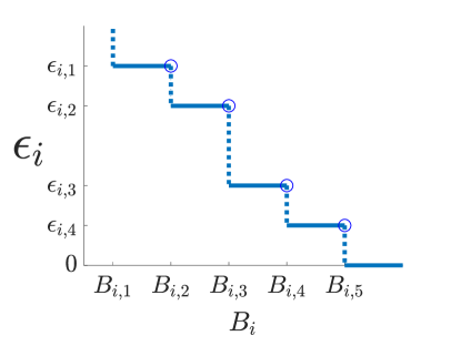
Figure 1: Illustration of step objective functions.

Then, we can formulate the MECB problem in the distributed setting (MECBD) as follows:

$$\min\quad {\max_{i\in\{1,\ldots,N\}}}\epsilon_{i}(B_{i})$$ (14a)

s.t. $$\sum_{i=1}^{N}B_{i}\leq B.$$ (14b)

Note that to compute $\epsilon_{i}(B_{i})$ for a given $B_{i}$, we need to solve an instance of the MECB problem in (10) for dataset $\mathcal{Y}_{i}$ and budget $B_{i}$.

input : Distributed datasets $\{\mathcal{Y}_{i}\}_{i=1}^{N}$, Lipschitz constant $\rho$, communication budget $B$.

output : Optimal $\{(k^{*}_{i},b^{*}_{i})\}_{i=1}^{N}$ to configure the construction of local quantized coresets within a global budget $B$.

1

each node $i=1,...,N$:  

2       $B_{0}\leftarrow 1\cdot(1+m_{e})\cdot d$;

3       compute $\epsilon_{i}(B_{0})$ by MD-MECB or EVD-MECB;

4       $\mathcal{E}_{i}\leftarrow\{(B_{0},\epsilon_{i}(B_{0}))\}$;

5       foreach integer $B_{i}\in[B_{0}+1,|\mathcal{Y}_{i}|\cdot b_{0}\cdot d]$ do

6             compute $\epsilon_{i}(B_{i})$ by MD-MECB or EVD-MECB;

7             if $\epsilon_{i}(B_{i})<\min\{\epsilon_{i,j}:\>(B_{i,j},\epsilon_{i,j})\in\mathcal{E}_{i}\}$  then

8                   $\mathcal{E}_{i}\leftarrow\mathcal{E}_{i}\cup\{(B_{i},\epsilon_{i}(B_{i}))\}$;

9                  

10      report $\mathcal{E}_{i}$ to the server;

the server:  

11       $\mathbf{E}$ is an ordered list of $\epsilon$-values in $\bigcup_{i}\mathcal{E}_{i}$, sorted in descending order;

12       $I_{max}\leftarrow$ first index in $\mathbf{E}$;

13       $I_{min}\leftarrow$ last index in $\mathbf{E}$;

14       while true  do

15             $I\leftarrow\Bigl{\lfloor}\frac{I_{max}+I_{min}}{2}\Bigr{\rfloor}$;

16             $\epsilon_{I}\leftarrow$ the $I$-th element in $\mathbf{E}$;

17             for $i=1,\ldots,N$  do

18                   $B_{i}(\epsilon_{I})\leftarrow\min\{B_{i,j}:\>(B_{i,j},\epsilon_{i,j})\in\mathcal{E}_{i},\>\epsilon_{i,j}\leq\epsilon_{I}\}$;

19                  

20             if $I_{min}=I_{max}+1$  then

21                   send $B_{i}(\epsilon_{I})$ to node $i$ for each $i=1,\ldots,N$;

22                   break while loop;

23                  

24            else

25                   if $\sum_{i=1}^{N}B_{i}(\epsilon_{I})>B$ then

26                         $I_{min}=I$;

27                        

28                  else

29                         $I_{max}=I$;

30                        

31                  

32      

each node $i=1,...,N$:  

33       find local $(k_{i}^{*},b_{i}^{*})$ under budget $B_{i}(\epsilon_{I})$ given by the server by MD-MECB or EVD-MECB;

34      

35return $\{(k^{*}_{i},b^{*}_{i})\}_{i=1}^{N}$;

Algorithm 4 OBA-MECBD

VI-B Optimal Budget Allocation Algorithm for MECBD (OBA-MECBD)

The MECBD problem in (14) is a minimax knapsack problem [45, 46] with a nonlinear non-increasing objective function. Special cases of this problem with strictly decreasing objective functions have been solved in [46]. However, the objective function of MECBD is a step function as shown below, which is not strictly decreasing. Below we will develop a polynomial-time algorithm to solve our instance of the minimax knapsack problem using the following property of $\epsilon_{i}(B_{i})$.

We note that $\epsilon_{i}(B_{i})$ is a non-increasing step function of $B_{i}$ (see Figure 1). This is because the configuration parameters $k$ and $b$ in the CS + QT procedure are integers. Therefore, there exist intervals $[B_{i,j},B_{i,j+1})$ ($j=0,1,2,...$) such that for any $B_{i},B^{\prime}_{i}\in[B_{i,j},B_{i,j+1})$, we have $\epsilon_{i}(B_{i})=\epsilon_{i}(B^{\prime}_{i})$, as shown in Figure 1. Given a target value of $\epsilon_{i}$, the minimum $B_{i}$ for reaching this target is thus always within the set $\{B_{i,j}\}$.

Our algorithm, shown in Algorithm 4, has three main steps. First, in lines 4–4, each node computes the set $\mathcal{E}_{i}$ of all pairs of $B_{i,j}$ and the corresponding $\epsilon_{i}(B_{i,j})$. This is achieved by evaluating $\epsilon_{i}(B_{i})$ according to MD-MECB or EVD-MECB for gradually increasing $B_{i}$ and recording all the points where $\epsilon_{i}(\cdot)$ decreases. After that, the set $\mathcal{E}_{i}$ is sent to a server.

Second, the server allocates the global budget to the nodes according to lines 4–4. To this end, it computes an ordered list $\mathbf{E}$ of all possible values of the global $\epsilon:=\max_{i}\epsilon_{i}$. Let $B_{i}(\epsilon)$ denote the smallest value of $B_{i}$ such that $\epsilon_{i}(B_{i})\leq\epsilon$. The main idea is to perform a binary search for the target value of $\epsilon\in\mathbf{E}$ (lines 4–4). For each candidate value of $\epsilon$, we compute $B_{i}(\epsilon)$ for all $i$. If $\sum_{i}B_{i}(\epsilon)<B$ (i.e., we are below the budget when targeting at the current choice of $\epsilon$), we will eliminate all $\epsilon^{\prime}\in\mathbf{E}$ such that $\epsilon^{\prime}>\epsilon$; otherwise, we will eliminate all $\epsilon^{\prime}\in\mathbf{E}$ such that $\epsilon^{\prime}<\epsilon$. After finding the target value of $\epsilon$ such that $\sum_{i}B_{i}(\epsilon)$ achieves the largest value within $B$, the server sends the corresponding local budget $B_{i}(\epsilon)$ to each node.

Finally, each node uses MD-MECB or EVD-MECB to compute its local configuration $(k_{i}^{*},b_{i}^{*})$ under the given budget.

Complexity: We analyze the complexity step by step. First, computing $\mathcal{E}_{i}$ at each node (lines 4–4) has a complexity of $O((n^{2}+b_{0})db_{0}n)$ if using MD-MECB and $O((n^{3}+d+b_{0})db_{0}n)$ if using EVD-MECB, dominated by line 4. Second, computing the budget allocation at the server (lines 4–4) has a complexity of $O(db_{0}n\log(db_{0}n))$. Specifically, as $\mathbf{E}$ has $O(db_{0}n)$ elements, sorting it takes $O(db_{0}n\log(db_{0}n))$. The while loop is repeated $O(\log(db_{0}n))$ times, as each loop eliminates half of the candidate $\epsilon$ values in $\mathbf{E}$, and each loop takes $O(db_{0}n)$, dominated by lines 4–4. Finally, computing the local configuration at each node (line 4) takes $O(n^{2}+b_{0})$ using MD-MECB and $O(n^{3}+d+b_{0})$ using EVD-MECB.

Optimality: Next, we prove the optimality of OBA-MECBD in budget allocation. Let $\epsilon_{i}^{\pi}(B_{i})$ be the error bound for a given solution $\pi$ of the MECB problem for dataset $\mathcal{Y}_{i}$ and budget $B_{i}$. We show that OBA-MECBD is optimal in the following sense.

Theorem VI.1.

Using a given MECB algorithm $\pi$ as the subroutine called in lines 4, 4, and 4, OBA-MECBD solves MECBD optimally w.r.t. $\pi$, i.e., its budget allocation $(B_{i})_{i=1}^{N}$ is the optimal solution to (14) with $\epsilon_{i}(B_{i})$ replaced by $\epsilon_{i}^{\pi}(B_{i})$.

Proof.

Let $B_{i}^{\pi}(\epsilon)$ denote the smallest value of $B_{i}$ such that $\epsilon_{i}^{\pi}(B_{i})\leq\epsilon$. By lines 4–4 in Algorithm 4, $I_{min}$ and $I_{max}$ should always satisfy $\sum_{i=1}^{N}B_{i}^{\pi}(\epsilon_{I_{min}})>B$ and $\sum_{i=1}^{N}B_{i}^{\pi}(\epsilon_{I_{max}})\leq B$ for all nontrivial values of $B$. Let $\epsilon^{*}$ denote the value of $\epsilon_{I}$ at the end of budget allocation, which is the value of (14a) achieved by OBA-MECBD. As $I=I_{max}$ and $I_{min}=I_{max}+1$ at this time, $\epsilon^{*}$ must be the smallest value of $\epsilon$ such that $\sum_{i=1}^{N}B_{i}^{\pi}(\epsilon)\leq B$. Therefore, for any other budget allocation $(B^{\prime}_{i})_{i=1}^{N}$ such that $\sum_{i=1}^{N}B^{\prime}_{i}\leq B$, we must have $\max_{i}\epsilon_{i}^{\pi}(B^{\prime}_{i})\geq\epsilon^{*}$. ∎

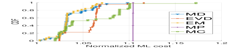
(a) MEB

(b) $k$-means ($k=2$)

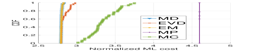
(c) PCA (3 components)

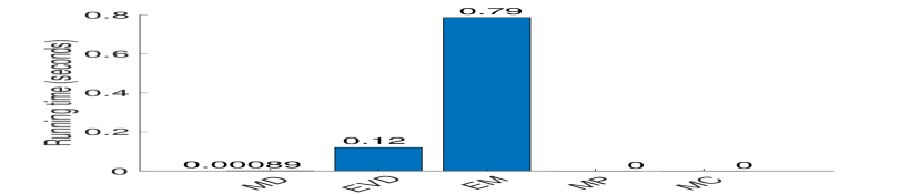
(d) Running time

Figure 2: Evaluation on Fisher’s Iris dataset (centralized setting).

VII Performance Evaluation

In this section, we evaluate our proposed algorithms using multiple real-world datasets for various ML tasks. Our objective is to validate the effectiveness and efficiency of our proposed algorithms (EVD-MECB, MD-MECB, OBA-MECBD) against benchmarks.

VII-A Datasets

In our experiments, we use four real-world datasets to evaluate our algorithms: (1) Fisher’s Iris dataset [47], with 3 classes, 50 data points in each class, 5 attributes for each data point; (2) Facebook metric dataset [48], which has 494 data points with 19 attributes; (3) Pendigits dataset [49], which has $7,494$ data points and 17 attributes; (4) MNIST handwritten digits dataset in a 784-dimensional space [50], where we use $60,000$ data points for training and $10,000$ data points for testing. We leverage the approach in [16] to pre-process the labels, i.e., each label is mapped to a number such that distance between points with the same label is smaller than distance between points with different labels. All the original data are represented in the standard IEEE 754 double-precision binary floating-point format [35].

VII-B ML Tasks

We consider four ML tasks: (1) minimum enclosing ball (MEB) [9]; (2) $k$-means ($k=2$ in our experiments); (3) principal component analysis (PCA); and (4) neural network (NN) (with three layers, 100 neurons in the hidden layer). Tasks (1–3) are unsupervised, and task (4) is supervised.

VII-C Algorithms

For the centralized setting, we consider five different algorithms for comparison. The first two are the proposed algorithms, i.e., EVD-MECB in Algorithm 1 (denoted by EVD), MD-MECB in Algorithm 3 (denoted by MD). The third algorithm is the straightforward solution EM (see Section IV-C3). The fourth algorithm aims to Maximize the Precision (MP), i.e., using the configuration $k=\Bigl{\lfloor}\frac{B}{d\cdot b_{0}}\Bigr{\rfloor}$ and $b=b_{0}$ to construct coresets. The fifth algorithm aims to Maximize the Cardinality (MC), i.e., using $k=\min(n,\Bigl{\lfloor}\frac{B}{d\cdot(1+m_{e})}\Bigr{\rfloor})$ and $b=\max(1+m_{e},\Bigl{\lfloor}\frac{B}{d\cdot n}\Bigr{\rfloor})$ to construct coresets, where $1+m_{e}$ is the minimum number of bits required to represent a number by the rounding-based quantizer (Section III-C).

For the distributed setting, we consider six algorithms for comparison. The first five algorithms correspond to instances of OBA-MECBD in Algorithm 4 that use EVD-MECB, MD-MECB, EM, MP, and MC as their subroutines, respectively. We denote these algorithms by OBA-EVD, OBA-MD, OBA-EM, OBA-MP and OBA-MC, respectively. The sixth algorithm is DRCC as proposed in [16] that optimizes the allocation of a given coreset cardinality to individual nodes.

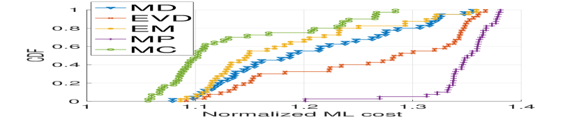
(a) MEB

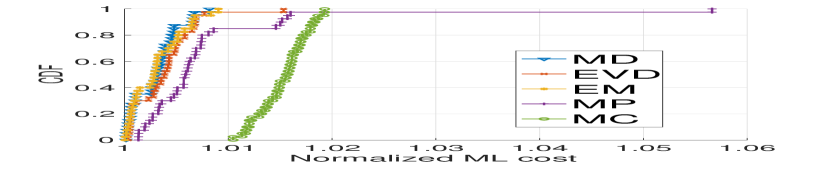
(b) $k$-means ($k=2$)

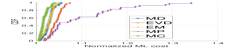
(c) PCA (3 components)

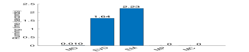
(d) Running time

Figure 3: Evaluation on Facebook metric dataset (centralized setting).

VII-D Performance Metrics

We use the normalized ML cost to measure the performance of unsupervised ML tasks. The normalized ML cost is defined as $\mbox{cost}(\mathcal{Y},\mathbf{x}_{\mathcal{S}})/\mbox{cost}(\mathcal{Y},\mathbf{x}^{*})$, where $\mathbf{x}_{\mathcal{S}}$ is the model learned from coreset $\mathcal{S}$ and $\mathbf{x}^{*}$ is the model learned from the original dataset $\mathcal{Y}$. For supervised ML tasks, we use classification accuracy to measure the performance. Furthermore, we report the running time of each algorithm. All metrics are computed over $40$ Monte Carlo runs unless stated otherwise.

VII-E Results in Centralized Setting

VII-E1 Unsupervised Learning

We first evaluate the unsupervised learning tasks: MEB, $k$-means, and PCA. We perform this evaluation on three datasets: Fisher’s Iris, Facebook metric, and Pendigits. Figures 2–4 show the cumulative distribution function (CDF) of normalized ML costs as well as the average running time of each algorithm, when the budget is set to $2\%$ of the size of the original dataset, i.e., $B=960$, $12014$ and $163069$, respectively. We also list the $b^{*}$ values over the Monte Carlo runs for EVD-MECB (EVD), MD-MECB (MD), and EM in Tables II–IV. We have the following observations: 1) In most cases, our proposed algorithms EVD-MECB and MD-MECB yield coresets that are much smaller ($98\%$ smaller) than the original dataset but support these ML tasks with less than $10\%$ degradation in performance. 2) Compared to the proposed algorithms, EM achieves a slightly better ML performance, but has a much higher running time. 3) Compared to EVD-MECB, MD-MECB is not only faster, but also more closely approximates EM. 4) Compared with MP and MC that relies on a single operation, the algorithms jointly optimizing coreset constrution and quantization (EM, EVD-MECB, MD-MECB) achieve much better ML performance over all.

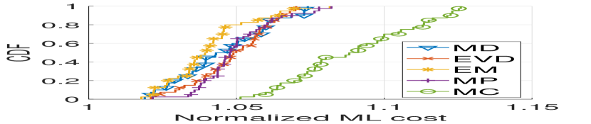
(a) MEB

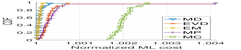
(b) $k$-means ($k=2$)

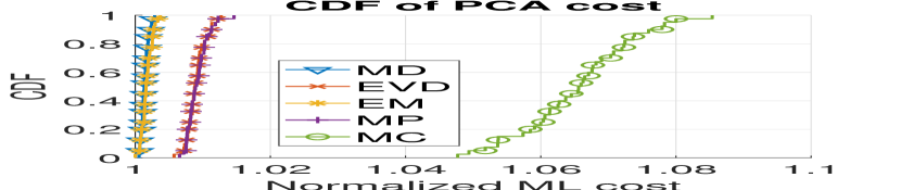
(c) PCA (11 components)

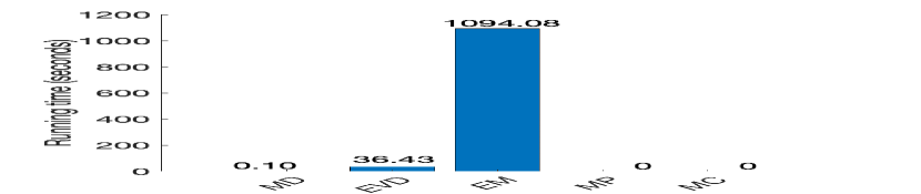
(d) Running time

Figure 4: Evaluation on Pendigits dataset (centralized setting).

TABLE II: Returned $b^{*}$ for Fisher’s Iris

Algorithm	$b^{*}$	$\#$ of occurrences
EVD	[31]	[40]
MD	$[16,18,20,23]$	$[1,22,16,1]$
EM	$[18,20]$	$[21,19]$

TABLE III: Returned $b^{*}$ for Facebook Metric

Algorithm	$b^{*}$	$\#$ of occurrences
EVD	[20]	[40]
MD	$[18,19,20,21,22,23]$	$[3,5,20,6,4,2]$
EM	$[18,19,20,21,22,23,24,27]$	$[1,6,9,6,10,5,2,1]$

TABLE IV: Returned $b^{*}$ for Pendigits

Algorithm	$b^{*}$	$\#$ of occurrences
EVD	[52]	[40]
MD	$[19,20,21]$	$[4,35,1]$
EM	$[19,20,21,22,23,24]$	$[5,15,6,7,6,1]$

VII-E2 Supervised Learning

For supervised learning, we evaluate neural network based classification on the MNIST dataset. We do not evaluate EM here because its running time for this dataset is prohibitively high.

Same as unsupervised learning, we only use $2\%$ of the original data, i.e., $B=60,211,200$. Figure 5 shows the CDFs of classification accuracy over 10 Monte Carlo runs. Note that in contrast to costs, a higher accuracy means better performance. MD-MECB, EVD-MECB, and MP all achieve over $80\%$ accuracy, while MC only achieves less than $40\%$ accuracy, because it changes the value of each attribute too much. As we zoom in, we see that MD-MECB performs the best. Moreover, MD-MECB is also relatively fast, with a running time of approximately $15$ minutes per run, whereas EVD-MECB takes up to $4.5$ hours for each run due to computing eigenvalue decomposition for a large matrix. After evaluating different budgets, we note that although MP happens to perform well with $2\%$ data, its performance is highly sensitive to the budget $B$, while the proposed algorithms (MD-MECB, EVD-MECB) adapt well to a wide range of budgets.

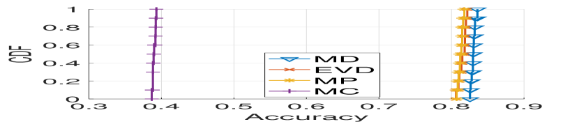
(a) Overall CDFs

(b) Zoomed-in CDFs

Figure 5: Evaluation on MNIST (Neural Net Accuracies)

VII-F Results in Distributed Setting

In this experiment, we use Fisher’s Iris dataset and Pendigits dataset to evaluate our proposed distributed algorithm (Algorithm 4). The original data points are randomly distributed across 10 nodes. The global communication budgets are set to $4,875$ bits for Fisher’s Iris and $828,087$ bits for Pendigits, which correspond to $10\%$ of the original data size.

We present the results for distributed setting in Figures LABEL:fig:fisheriris_distributed and LABEL:fig:pendigits_distributed, from which we have the following observations: 1) With only $10\%$ data in the distributed setting, most of the algorithms equipped with OBA outperform DRCC with a small degradation in the ML performance. 2) Compared with OBA-MP, OBA-MC, and DRCC that only rely on one operation to compress the data, our proposed OBA-EVD and OBA-MD which jointly optimize the operations of coreset construction and quantization perform significantly better. 3) OBA-MD is the most efficient over all these algorithms.

VII-G Summary of Experimental Results

• We demonstrate via real ML tasks and datasets that it is possible to achieve reasonable ML performance (less than $10\%$ of degradation in most cases) and substantial data reduction ($90$–$98\%$ smaller than the original dataset) by combining coreset construction with quantization.

• The proposed algorithms approximate the performance of EM, with a significantly lower running time.

• Jointly optimizing coreset construction and quantization achieves much better ML performance than relying on only one of these operations.

• MD-MECB and its distributed variant (OBA-MD) achieve the best performance-efficiency tradeoff among all the evaluated algorithms, making them the most suitable for large datasets.

VIII Conclusion

In this paper, we have proposed the first framework, MECB, to jointly configure coreset construction algorithms and quantizers in order to minimize the ML error under a given communication budget. We have proposed two algorithms to efficiently compute approximate solutions to the MECB problem, whose effectiveness and efficiency have been demonstrated through experiments based on multiple real-world datasets. We have further proposed an algorithm to extend our solutions to the distributed setting by carefully allocating the communication budget across multiple nodes to minimize the overall ML error, which has shown significant improvements over alternatives when combined with our proposed solutions to MECB. Our solutions only depend on a smoothness parameter of the ML cost function, and can thus serve as a key enabler in reducing the communication cost for a broad range of ML tasks.

References

- [1] J. Konečnỳ, H. B. McMahan, F. X. Yu, P. Richtárik, A. T. Suresh, and D. Bacon, “Federated learning: Strategies for improving communication efficiency,” arXiv preprint arXiv:1610.05492, 2016.
- [2] V. Smith, C.-K. Chiang, M. Sanjabi, and A. S. Talwalkar, “Federated multi-task learning,” in Advances in Neural Information Processing Systems, 2017, pp. 4424–4434.
- [3] S. Wang, T. Tuor, T. Salonidis, K. K. Leung, C. Makaya, T. He, and K. Chan, “When edge meets learning: Adaptive control for resource-constrained distributed machine learning,” in IEEE INFOCOM 2018-IEEE Conference on Computer Communications. IEEE, 2018, pp. 63–71.
- [4] J. M. Phillips, “Coresets and sketches,” arXiv preprint arXiv:1601.00617, 2016.
- [5] D. Feldman, M. Monemizadeh, C. Sohler, and D. P. Woodruff, “Coresets and sketches for high dimensional subspace approximation problems,” in Proceedings of the twenty-first annual ACM-SIAM symposium on Discrete Algorithms. Society for Industrial and Applied Mathematics, 2010, pp. 630–649.
- [6] T. Sarlos, “Improved approximation algorithms for large matrices via random projections,” in 2006 47th Annual IEEE Symposium on Foundations of Computer Science (FOCS’06). IEEE, 2006, pp. 143–152.
- [7] M. Bādoiu, S. Har-Peled, and P. Indyk, “Approximate clustering via core-sets,” in ACM STOC, 2002.
- [8] P. K. Agarwal, S. Har-Peled, and K. R. Varadarajan, “Geometric approximation via coresets,” Combinatorial and computational geometry, vol. 52, pp. 1–30, 2005.
- [9] K. L. Clarkson, “Coresets, sparse greedy approximation, and the frank-wolfe algorithm,” ACM Transactions on Algorithms (TALG), vol. 6, no. 4, p. 63, 2010.
- [10] S. Har-Peled and S. Mazumdar, “On coresets for k-means and k-median clustering,” in Proceedings of the thirty-sixth annual ACM symposium on Theory of computing. ACM, 2004, pp. 291–300.
- [11] D. Feldman and M. Langberg, “A unified framework for approximating and clustering data,” in STOC, June 2011.
- [12] M. F. Balcan, S. Ehrlich, and Y. Liang, “Distributed k-means and k-median clustering on general topologies,” in NIPS, 2013.
- [13] D. Feldman, M. Volkov, and D. Rus, “Dimensionality reduction of massive sparse datasets using coresets,” in NIPS, 2016.
- [14] M. Langberg and L. J. Schulman, “Universal approximators for integrals,” in SODA, 2010.
- [15] D. Feldman, M. Schmidt, and C. Sohler, “Turning big data into tiny data: Constant-size coresets for k-means, PCA, and projective clustering,” in SODA, 2013.
- [16] H. Lu, M.-J. Li, T. He, S. Wang, V. Narayanan, and K. S. Chan, “Robust coreset construction for distributed machine learning,” 2019. [Online]. Available: http://arxiv.org/abs/1904.05961
- [17] R. M. Gray and D. L. Neuhoff, “Quantization,” IEEE transactions on information theory, vol. 44, no. 6, pp. 2325–2383, 1998.
- [18] S. Lloyd, “Least squares quantization in pcm,” IEEE transactions on information theory, vol. 28, no. 2, pp. 129–137, 1982.
- [19] K. Sayood, Introduction to Data Compression, Fourth Edition, 4th ed. San Francisco, CA, USA: Morgan Kaufmann Publishers Inc., 2012.
- [20] T. Fischer, “A pyramid vector quantizer,” IEEE transactions on information theory, vol. 32, no. 4, pp. 568–583, 1986.
- [21] D. Goodman and R. Wilkinson, “A robust adaptive quantizer,” IEEE Transactions on Communications, vol. 23, no. 11, pp. 1362–1365, 1975.
- [22] N. Farvardin and V. Vaishampayan, “Optimal quantizer design for noisy channels: An approach to combined source-channel coding,” IEEE Transactions on Information Theory, vol. 33, no. 6, pp. 827–838, 1987.
- [23] A. Dasgupta, P. Drineas, B. Harb, R. Kumar, and M. W. Mahoney, “Sampling algorithms and coresets for ell_p regression,” SIAM Journal on Computing, vol. 38, no. 5, pp. 2060–2078, 2009.
- [24] M. Lucic, M. Faulkner, A. Krause, and D. Feldman, “Training mixture models at scale via coresets,” stat, vol. 1050, p. 23, 2017.
- [25] K. Chen, “On coresets for k-median and k-means clustering in metric and euclidean spaces and their applications,” SIAM Journal on Computing, vol. 39, no. 3, pp. 923–947, 2009.
- [26] D. Feldman, M. Feigin, and N. Sochen, “Learning big (image) data via coresets for dictionaries,” Journal of mathematical imaging and vision, vol. 46, no. 3, pp. 276–291, 2013.
- [27] C. Boutsidis, P. Drineas, and M. Magdon-Ismail, “Near-optimal coresets for least-squares regression,” IEEE. Trans. IT, vol. 59, no. 10, pp. 6880–6892, October 2013.
- [28] S. Har-Peled and S. Mazumdar, “On coresets for k-means and k-median clustering,” in STOC, 2004.
- [29] K. L. Clarkson, “Coresets, sparse greedy approximation, and the Frank-Wolfe algorithm,” ACM Transactions on Algorithms, vol. 6, no. 4, August 2010.
- [30] S. Han, H. Mao, and W. J. Dally, “Deep compression: Compressing deep neural networks with pruning, trained quantization and huffman coding,” arXiv preprint arXiv:1510.00149, 2015.
- [31] A. Zhou, A. Yao, Y. Guo, L. Xu, and Y. Chen, “Incremental network quantization: Towards lossless cnns with low-precision weights,” arXiv preprint arXiv:1702.03044, 2017.
- [32] D. Lin, S. Talathi, and S. Annapureddy, “Fixed point quantization of deep convolutional networks,” in International Conference on Machine Learning, 2016, pp. 2849–2858.
- [33] R. M. Gray, “Vector quantization,” Readings in speech recognition, vol. 1, no. 2, pp. 75–100, 1990.
- [34] A. Gersho and R. M. Gray, Vector quantization and signal compression. Springer Science & Business Media, 2012, vol. 159.
- [35] IEEE, “754-2019 - ieee standard for floating-point arithmetic,” 2019. [Online]. Available: https://ieeexplore.ieee.org/servlet/opac?punumber=8766227
- [36] D. Arthur and S. Vassilvitskii, “k-means++: The advantages of careful seeding,” in SODA, January 2007.
- [37] C. Ding and X. He, “K-means clustering via principal component analysis,” in Proceedings of the twenty-first international conference on Machine learning. ACM, 2004, p. 29.
- [38] G. W. Stewart, “A krylov–schur algorithm for large eigenproblems,” SIAM Journal on Matrix Analysis and Applications, vol. 23, no. 3, pp. 601–614, 2002.
- [39] A. Lim, B. Rodrigues, F. Wang, and Z. Xu, “k-center problems with minimum coverage,” Theoretical Computer Science, vol. 332, no. 1-3, pp. 1–17, 2005.
- [40] S. Khuller and Y. J. Sussmann, “The capacitated k-center problem,” SIAM Journal on Discrete Mathematics, vol. 13, no. 3, pp. 403–418, 2000.
- [41] S. Khuller, R. Pless, and Y. J. Sussmann, “Fault tolerant k-center problems,” Theoretical Computer Science, vol. 242, no. 1-2, pp. 237–245, 2000.
- [42] D. S. Hochbaum and D. B. Shmoys, “A best possible heuristic for the k-center problem,” Mathematics of operations research, vol. 10, no. 2, pp. 180–184, 1985.
- [43] J. Kleinberg and E. Tardos, Algorithm design. Pearson Education India, 2006.
- [44] J. Demmel, I. Dumitriu, and O. Holtz, “Fast linear algebra is stable,” Numerische Mathematik, vol. 108, no. 1, pp. 59–91, 2007.
- [45] H. Luss, “A nonlinear minimax allocation problem with multiple knapsack constraints,” Operations Research Letters, vol. 10, no. 4, pp. 183–187, 1991.
- [46] ——, “An algorithm for separable non-linear minimax problems,” Operations Research Letters, vol. 6, no. 4, pp. 159–162, 1987.
- [47] R. Fisher, “Iris data set,” https://archive.ics.uci.edu/ml/datasets/iris, 1936. [Online]. Available: https://archive.ics.uci.edu/ml/datasets/iris
- [48] S. Moro, P. Rita, and B. Vala, “Facebook metrics data set,” https://archive.ics.uci.edu/ml/datasets/Facebook+metrics, 2016. [Online]. Available: https://archive.ics.uci.edu/ml/datasets/Facebook+metrics
- [49] E. Alpaydin and F. Alimoglu, “Pen-based recognition of handwritten digits data set,” https://archive.ics.uci.edu/ml/datasets/Pen-Based+Recognition+of+Handwritten+Digits, 1996. [Online]. Available: https://archive.ics.uci.edu/ml/datasets/Pen-Based+Recognition+of+Handwritten+Digits
- [50] Y. LeCun, C. Cortes, and C. Burges, “The MNIST database of handwritten digits,” http://yann.lecun.com/exdb/mnist/, 1998. [Online]. Available: http://yann.lecun.com/exdb/mnist/