Discovery and analysis of three magnetic hot subdwarf stars: evidence for merger-induced magnetic fields

Abstract

Magnetic fields can play an important role in stellar evolution. Among white dwarfs, the most common stellar remnant, the fraction of magnetic systems is more than 20 per cent. The origin of magnetic fields in white dwarfs, which show strengths ranging from 40 kG to hundreds of MG, is still a topic of debate. In contrast, only one magnetic hot subdwarf star has been identified out of thousands of known systems. Hot subdwarfs are formed from binary interaction, a process often associated with the generation of magnetic fields, and will evolve to become white dwarfs, which makes the lack of detected magnetic hot subdwarfs a puzzling phenomenon. Here we report the discovery of three new magnetic hot subdwarfs with field strengths in the range 300–500 kG. Like the only previously known system, they are all helium-rich O-type stars (He-sdOs). We analysed multiple archival spectra of the three systems and derived their stellar properties. We find that they all lack radial velocity variability, suggesting formation via a merger channel. However, we derive higher than typical hydrogen abundances for their spectral type, which are in disagreement with current model predictions. Our findings suggest a lower limit to the magnetic fraction of hot subdwarfs of $0.147^{+0.143}_{-0.047}$ per cent, and provide evidence for merger-induced magnetic fields which could explain white dwarfs with field strengths of $50-150$ MG, assuming magnetic flux conservation.

1 Introduction

Magnetic fields have been detected in stars across many evolutionary stages, from the main sequence (Babcock, 1947) to the white dwarf cooling sequence (Kemp et al., 1970), since many decades. Yet the origin and evolution of these fields is not entirely understood (e.g. Ferrario et al., 2015; Wurster et al., 2018). For white dwarfs, the final observable evolutionary stage of over 95 per cent of stars, the fraction of systems with detectable magnetic fields is estimated to be over one fifth ($22\pm 4$ per cent, Bagnulo & Landstreet, 2021).

Several mechanisms have been put forward to explain the magnetic fields observed in white dwarfs. Firstly, the magnetic field could be explained simply as a fossil field that was already present in the cloud from which the star originally formed (Woltjer, 1964; Landstreet, 1967; Angel et al., 1981). In this scenario, the field strength results from flux conservation when the progenitor star contracts to become a white dwarf, with magnetic Ap and Bp stars (Moss, 2001) being the likely progenitors of magnetic white dwarfs. Alternatively, the fossil field could arise due to a dynamo acting in the convective core during the main sequence or the asymptotic giant branch (Stello et al., 2016) and only be revealed after the white dwarf progenitor loses its outer layers. Another model suggests that the magnetic field could result from a dynamo generated during the merger of two stars forming a white dwarf (Tout et al., 2008; Briggs et al., 2015, 2018), or from the merger of two white dwarfs (García-Berro et al., 2012). A merger during an earlier evolutionary stage (the main sequence or even pre-main sequence, Ferrario et al., 2009; Schneider et al., 2016; Schneider et al., 2019) leading to a magnetic main sequence star that evolves to a magnetic white dwarf is also a possibility. Finally, another scenario proposes that the magnetic fields in white dwarfs are generated during the cooling of the star itself (Valyavin & Fabrika, 1999), for example due to crystallisation, which induces the formation of a convective mantle around the solid white dwarf core (Isern et al., 2017). However, none of these scenarios alone can fully explain the observed fraction and field strengths of magnetic white dwarfs; likely more than one scenario is required (Bagnulo & Landstreet, 2021).

Before reaching the white dwarf stage, a small fraction of systems will go through the extended horizontal branch (EHB), where they are referred to as hot subdwarf stars (see Heber, 2016, for a review). These stars appear hot and smaller than canonical horizontal branch stars due to previous enhanced mass-loss attributed to binary interaction (Han et al., 2002, 2003; Pelisoli et al., 2020). They will evolve directly to the white dwarf cooling track without ascending the asymptotic giant branch. Despite this direct connection with white dwarfs, the fraction of magnetic hot subdwarfs seems to be much smaller than that of magnetic white dwarfs. Searches using spectropolarimetry found no evidence of magnetic fields in around 40 hot subdwarfs, even with detection limits as low as 1 to 2 kG (Landstreet et al., 2012; Mathys et al., 2012; Randall et al., 2015; Bagnulo et al., 2015). The picture is not much better for detection through Zeeman splitting: to date, out of around 6000 spectroscopically confirmed hot subdwarfs (Geier, 2020; Culpan et al., 2022), there is only one confirmed magnetic hot subdwarf (Dorsch et al., 2022). An earlier work by Heber et al. (2013) claimed a first detection and reported a magnetic field strength of 300–700 kG from Zeeman-split hydrogen and helium lines, but the reported star was never named or analysed in detail. In addition, the merger remnant J22564-5910 could host a magnetic field, but the observed spectral features could instead be explained by a disc (Vos et al., 2021). The detection of photometric variability consistent with spots could point towards a magnetic field for a number of hot subdwarfs (Jeffery et al., 2013; Geier et al., 2015; Balona et al., 2019; Momany et al., 2020), but the cause for variability and its possible connection to a magnetic field remains to be investigated. This conflict between an abundance of magnetic white dwarfs and a dearth of magnetic hot subdwarfs might contain clues about the possible channels leading to the formation of magnetic white dwarfs, and thus to the behaviour of magnetic fields throughout stellar evolution, calling for more investigation of possible magnetic fields in hot subdwarfs.

In this work, we report the discovery and characterisation of three magnetic hot subdwarfs: SDSS J041536.05+253857.1 SDSS J130346.61+264630.6, and SDSS J160325.52+341237.4 (henceforth J0415+2538, J1303+2646, J1603+3412, respectively). This discovery represents a significant increase in the number of known magnetic hot subdwarfs, and can shed light onto the origin and evolution of stellar magnetic fields.

2 Spectroscopic and photometric data

We identified the possible presence of a magnetic field in the three stars based on visual analysis of spectra taken with the Sloan Digital Sky Survey (SDSS, Eisenstein et al., 2011). The three targets were part of a sample of candidate white dwarfs identified by their colours, but were instead found to show narrower lines and very blue spectra consistent with hot subdwarfs (see Fig. 1). The strength of the helium lines compared to the hydrogen lines and the presence of He ii lines imply a He-sdO classification for all three objects. In addition, we identified hints of Zeeman splitting of the Balmer lines, caused by the magnetic field breaking azimutal symmetry.

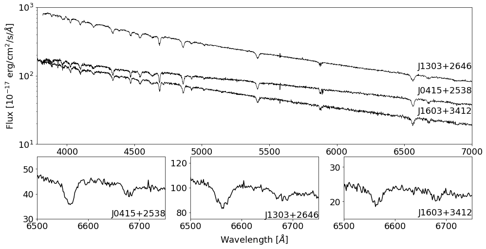
Figure 1: SDSS spectra of J0415+2538, J1303+2646, and J1603+3412 are shown in the top panel. The bottom panel zooms in the region around H $\alpha$ and the He i 6678 Å line, which show hints of Zeeman splitting. J0415+2538 is in a region with strong reddening (see Sec. 3.1).

We then searched the database of the Isaac Newton Group of telescopes for available spectroscopy for the three objects. We found multiple archival spectra taken with the Intermediate-dispersion Spectrograph and Imaging System (ISIS) at the William Herschel Telescope (WHT). Data from seven nights was available for J0415+2538 (Table 1), three nights for J1303+2646 (Table 2), and two for J1603+3412 (Table 3). In most cases, more than one spectrum was taken each night. For all observations, except those taken on 2015 December 15 for J0415+2538, arc lamps were taken in the same position as the target.

Table 1: List of archival WHT/ISIS spectra retrieved for J0415+2538

Date	Grating	Central wavelength (Å)		Number of spectra
		Blue	Red
20140203	R600	4300	6403	2
20140204	R600	4300	6403	2
20150822	R600	4298	6201	4
20150823	R600	4298	6201	4
20150824	R600	4298	6201	4
20150825	R600	4298	6201	4
20151215	R600	4498	6900	3

Table 2: List of archival WHT/ISIS spectra retrieved for J1303+2646

Date	Grating	Central wavelength (Å)		Number of spectra
		Blue	Red
20050225	R1200	4501	6199	1
20120531	R600	4351	6558	4
20150615	R1200	4750	6799	4
20150616	R1200	4750	6799	6

Table 3: List of archival WHT/ISIS spectra retrieved for J1603+3412

Date	Grating	Central wavelength (Å)		Number of spectra
		Blue	Red
20150615	R1200	4750	6799	4
20150616	R1200	4750	6799	5

We downloaded all the spectra and associated calibration files and performed data reduction and optimal extraction (Marsh, 1989) using pamela. All spectra were de-biased and flat-fielded using the standard starlink packages kappa, figaro and convert. Wavelength calibration was carried out using molly.

In order to search for photometric variability in the three stars, in particular variations that could be attributed to spots, we queried the database of the Transiting Exoplanet Survey Satellite (TESS, Ricker et al., 2015) using the Mikulski Archive for Space Telescopes (MAST). J0415+2538 (TIC 56742534) was observed in sectors 43 and 44 with cadences of 20 seconds and 2 minutes, whereas for J1303+2646 and J1603+3412 only 30-minute full-frame images (FFIs) are available during one and two sectors, respectively.

Though the cadence and duration of the TESS light curve is adequate for detecting rotation periods typical of most hot subdwarfs ($\lesssim 50$ days Charpinet et al., 2018; Reed et al., 2018), rotation periods nearing a hundred days have been detected for some hot subdwarfs (Reed et al., 2014; Bachulski et al., 2016). In addition, TESS observations can suffer from significant contamination from nearby stars given the large pixel size of 21 arcsec. In fact, the reported contribution of J0415+2538 to the TESS aperture is only 26 per cent. Only J1303+2646 seems to be fairly isolated, since the TESS observations of J1603+3412 are also possibly contaminated by a nearby bright star (see Fig. 2). For these reasons, we have also retrieved light curves from the Zwicky Transient Facility (ZTF, Bellm et al., 2019) and the Catalina Real Time Transient Survey (CRTS, Drake et al., 2009) for our three targets, given the better spatial resolution and often longer time span of these surveys compared to TESS.

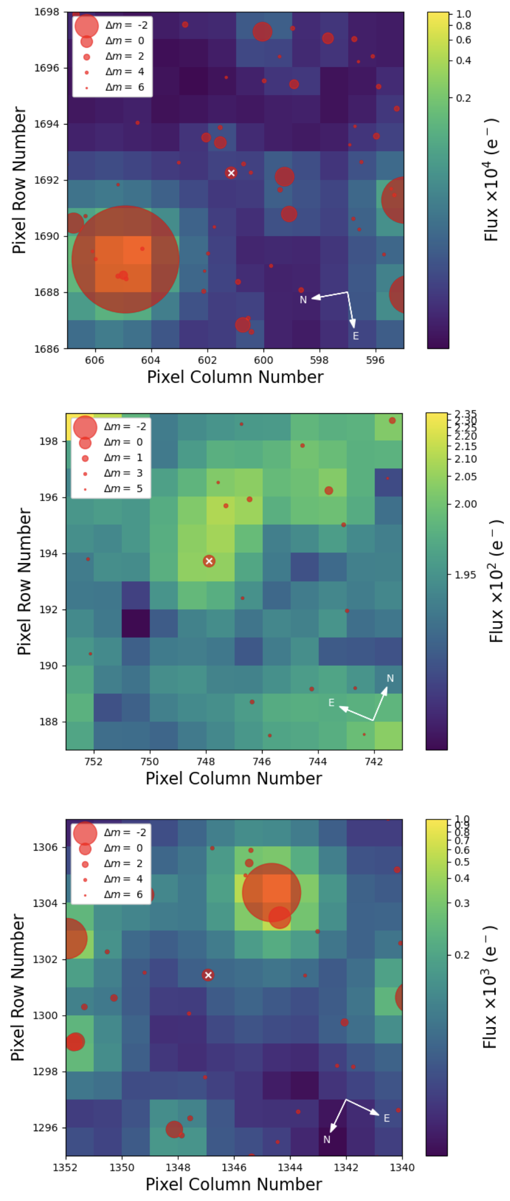
Figure 2: TESS field of view for the three targets, J0415+2538, J1303+2646, and J1603+3412 from top to bottom. The targets are marked by a white cross, and other stars in the field with a magnitude difference ($\Delta m$) of up to six are also indicated. Both J0415+2538 and J1603+3412 have bright stars nearby that likely contaminate their TESS light curves. Images generated with tpfplotter (Aller et al., 2020).

3 Data analysis

3.1 Spectral and spectral energy distribution fitting

The spectral analysis for our three targets was performed following the method used by Dorsch et al. (2022) to model the prototype magnetic He-sdO, Gaia DR2 5694207034772278400 (henceforth J0809-2627). Atmospheric structures were computed using the plane-parallel, homogeneous, and hydrostatic code Tlusty (Hubeny & Lanz, 2017a, b), including H, He, C, N, O, Ne, Si, P, S, Fe, and Ni in non-local thermodynamic equilibrium. The magnetic field was not considered in the atmospheric structure and only linear Zeeman splittings were included in the spectrum synthesis, which was performed with Synspec (Hubeny & Lanz, 2017c). A simple homogeneous and uniform magnetic field across the visible hemisphere was assumed. Polarised radiative transfer in the lines was not considered. A more detailed description of our methods is given in section 3 and appendix B of Dorsch et al. (2022).

We performed global $\chi^{2}$ fits to the WHT/ISIS spectra of each star. Initially we fitted the Doppler-corrected co-added spectra to evaluate the performance of our simple treatment of the magnetic field. The free parameters were the effective temperature $T_{\mathrm{eff}}$, the surface gravity $\log g$, the helium abundance $\log n(\mathrm{He})/n(\mathrm{H})$, and the mean magnetic field strength $B$. This initial fit showed that the spectra of J1303+2646 clearly display broadened displaced Zeeman components (see Fig. 3), which indicates that the magnetic field across the surface of this star is non-homogeneous. To account for that, we constructed toy models consisting of more than one homogeneous component, which allowed us to roughly emulate a non-homogeneous magnetic field geometry causing variation of the magnetic field strength on the stellar surface. For each star, we re-fitted the co-added spectra with one and two additional homogeneous magnetic field components that were allowed to vary in strength and surface ratio. The results of this exercise are summarised in Table 5. Importantly, our toy model also allowed us to investigate the systematic uncertainties of the derived atmospheric parameters caused by our approximation of an uniform magnetic field. The resulting $T_{\mathrm{eff}}$ values change insignificantly, because they are dominantly constrained by the helium ionisation equilibrium rather than by the detailed spectral line shapes. The surface gravities as well as the hydrogen to helium ratios, however, are derived mainly from the shapes of the hydrogen and helium lines. Therefore, changes of 0.1–0.2 dex are observed when introducing a second component. Adding a third one leads to considerably smaller changes of the atmospheric parameters, which we judge to be insignificant for J0415+2538 and J1603+3412, for which we therefore adopted the two-component model. The field structure of J1303+2646 is more complex, which led us to adopt three components.

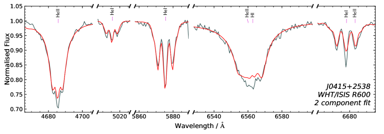
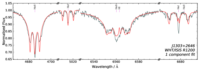
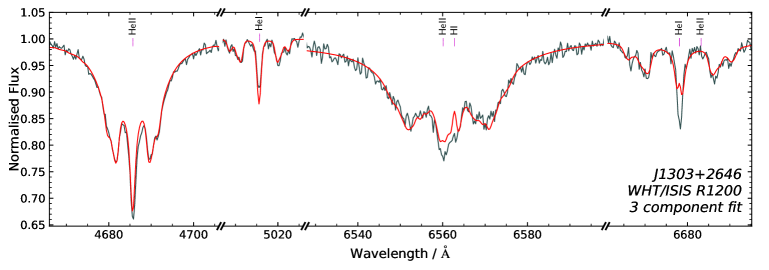
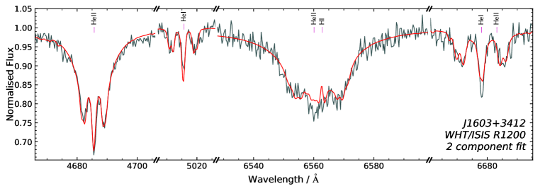
Figure 3: H i, He i and He ii lines in the merged and radial velocity-corrected WHT/ISIS spectra for each target. The best model is shown in red, not including metal lines. Labels indicate H i and He i-ii line positions at $B=0$. The top panel shows our best fit for J0415+2538. The two middle panels show fits for J1303+2646: initially using only one magnetic field component, which leads to a poor fit to the Zeeman components, and using three components, which can much better approximate the complex magnetic field geometry. The bottom panel shows the final fit for the merged spectrum of J1603+3412.

Once the number of components was fixed, all available spectra were fitted simultaneously with the selected number of components to determine $T_{\mathrm{eff}}$, $\log g$, $\log n(\mathrm{He})/n(\mathrm{H})$, mean magnetic field strength $B$ and surface ratio $A$ of each component, and the radial velocities $v_{\mathrm{rad}}$. We only allowed $v_{\mathrm{rad}}$ to be different for the individual spectra, forcing a global best-fit for the atmospheric parameters. The magnetic field axis was forced to be inclined at an angle $\psi=90^{\circ}$ with respect to the line of sight because our simplified model for the magnetic field geometry does not allow for a physical interpretation of this angle. The projected rotational velocity was fixed to $v_{\mathrm{rot}}\sin i$ = 0  km s^-1 for all stars because it is not well constrained by the low-resolution WHT/ISIS spectra. We only derived upper limits based on the value preferred by the fit. Spectral regions that were poorly reproduced by our models were excluded from the fit. This includes He i 4471 Å, as well as regions that are affected by metal lines. Important metal line blends are due to strong N iii lines partly blended with H i/He ii 4101, 4862 Å and He ii 4201, 4543 Å.

Our best-fit models are compared with the merged and radial velocity-corrected WHT/ISIS spectra in Fig. 3. The best-fit parameters are listed in Table 4, which lists the average magnetic field for each star. The strengths and relative surface ratios of the components are given in Table 6. The uncertainties of the atmospheric parameters stated in Table 4 are estimated systematical uncertainties because the statistical uncertainties are negligible in comparison. For the radial velocities, we state the average values and their standard deviations. For J0415+2538, we exclude the radial velocity measurements taken on 2015 December 15, given that no arc lamp was taken with the same pointing as the target, making the radial velocities unreliable due to instrumental shifts. In all three cases, there is no evidence of significant radial velocity variability in timescales spanning thousands of days (see Fig. 4), comparable to the longest orbital periods observed for hot subdwarfs (Vos et al., 2019), indicating that the three stars are single.

Table 4: Stellar parameters derived from spectroscopic and SED fits. We include also the values for the prototype star J0809-2627 from Dorsch et al. (2022) for comparison. For $T_{\mathrm{eff}}$, $\log g$, and $\log n(\mathrm{He})/n(\mathrm{H})$, we quote the systematic uncertainties which are dominant over the statistical ones. For $v_{\mathrm{rad}}$, we quote the average and standard deviation over the multiple measurements. For $R$ and $L$, the quoted values are the mode and the 68 per cent confidence interval.

	J0809-2627	J0415+2538	J1303+2646	J1603+3412
$T_{\mathrm{eff}}$ (K)	$44900\pm 1000$	$46580\pm 1500$	$47950\pm 1500$	$46450\pm 1500$
$\log g$	$\phantom{+}5.93\pm 0.15$	$\phantom{+}5.98\pm 0.25$	$\phantom{+}5.97\pm 0.30$	$\phantom{+}6.06\pm 0.20$
$\log n(\mathrm{He})/n(\mathrm{H})$	$+0.28\pm 0.10$	$-0.10\pm 0.15$	$+0.25\pm 0.15$	$+0.07\pm 0.15$
$B_{\mathrm{avg}}$ (kG)	$353\pm 10$	$305\pm 20$	$450\pm 20$	$335\pm 15$
$v_{\mathrm{rad}}$ (km s-1)	$33\pm 2$	$-17\pm 10$	$-37\pm 8$	$6\pm 5$
$v_{\mathrm{rot}}\sin i~{}$ (km s-1)	$<40$	$<45$	$<60$	$<65$
$R$ (R☉)	$0.184^{+0.011}_{-0.010}$	$0.148^{+0.020}_{-0.015}$	$0.19^{+0.05}_{-0.04}$	$0.14^{+0.06}_{-0.04}$
$L$ (L☉)	$123^{+19}_{-16}$	$91^{+29}_{-21}$	$160^{+100}_{-60}$	$70^{+80}_{-40}$

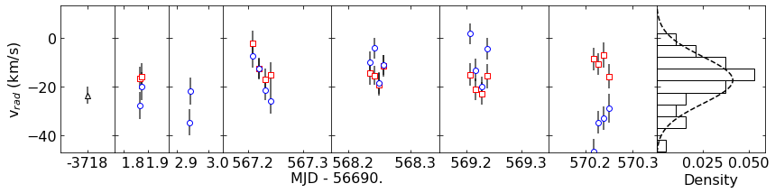
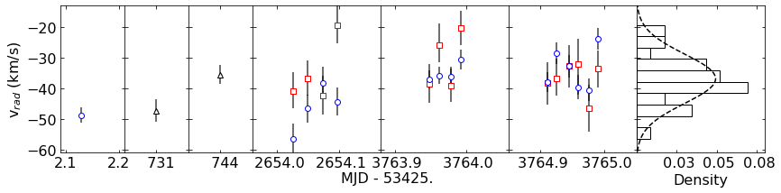
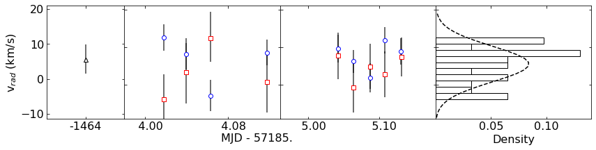
Figure 4: Radial velocities for J0415+2538, J1303+2646, and J1603+3412, from top to bottom. Estimates obtained from the red and blue WHT arms are shown as red squares and blue circles. Estimates from the SDSS spectra (two available in the case of J1303+2646) are shown as black triangles. The rightmost panel shows a histogram of the values, with a normal distribution with mean and standard deviation derived from the measurements for comparison.

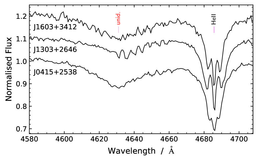
Figure 5: Merged and radial velocity-corrected WHT/ISIS spectra from top to bottom for J1603+3412, J1303+2646, and J0415+2538. The spectra are offset in steps of 0.1 for better visibility. The origin of the broad and smooth feature centred at about 4631 Å is unknown.

The similarities between the atmospheric parameters of all four known magnetic He-sdOs are remarkable. All stars share an intermediate helium abundance, with almost the same number of hydrogen and helium atoms in their photospheres. This is highly unusual for He-sdO stars at $T_{\mathrm{eff}}$ > 43 000 K, which are almost always extremely hydrogen-poor or helium-poor (Stroeer et al., 2007; Luo et al., 2021). The distinction of two groups of He-sdOs based on hydrogen abundance was suggested by Naslim et al. (2013), who named those with significant hydrogen (H/He $>$ 0.25), like our objects, intermediate He-sdO (iHe-sdO). Those with lower hydrogen content are called extreme He-sdO (eHe-sdO). An additional subdivision was proposed by Stroeer et al. (2007) and Hirsch (2009), who demonstrated that the He-sdOs from the ESO supernovae type Ia progenitor survey (SPY) project can be split into four groups characterised by their carbon and nitrogen content: N-rich, C-rich, C&N-rich, and N-poor objects. Due to the low resolution of the available spectra, detailed abundance patterns could not be determined. All stars seem to lack strong carbon lines, similar to J0809-2627. Hints of the C iv lines at 5805 Å and the C iii 4070 Å triplet are observed in the merged WHT/ISIS spectrum of J0415+2538 and to a lesser degree in the SDSS spectrum of J1603+3412, but are absent in the WHT/ISIS spectrum of J1303+2646. This suggests that carbon is not strongly enriched, although solar carbon abundances cannot be excluded. The N iii 4517, 4639 Å multiplets in the WHT/ISIS spectra of J1303+2646 are best reproduced at a nitrogen abundance of about ten times solar. The same lines are weaker in the spectra of J0415+2538 and J1603+3412, suggesting nitrogen abundances between two and six times solar. In short, there is indication that the magnetic objects are N-rich, but better spectra are needed to probe the C content.

In addition, all stars show a strong and broad feature in the 4629 – 4660 Å range, centred at about 4631 Å (see Fig. 5). The origin of the feature remains unclear. A photospheric origin seems to be excluded by the lack of similar features at other wavelengths. The same argument can be used to exclude both ultra-high excitation lines, which are observed for some DO-type white dwarfs (Werner et al., 1995; Reindl et al., 2019), and diffuse interstellar bands. An instrumental effect is excluded because the feature is also observed in the SDSS spectra. The feature is present in the X-SHOOTER spectrum J0809-2627 as well, but weaker than in the three new stars.

Following Dorsch et al. (2022), we also fitted the spectral energy distribution (SED) of the three stars using the same model grid. The SED was constructed by collecting photometric measurements from multiple surveys (see Appendix B). $T_{\mathrm{eff}}$, $\log g$, and $\log n(\mathrm{He})/n(\mathrm{H})$ were fixed to the values determined from spectroscopy, and the angular diameter $\Theta$ was left as a free parameter. We used the law of Fitzpatrick et al. (2019) to account for interstellar extinction, with the colour excess $E_{44-55}$ left to vary freely, but keeping a fixed extinction parameter $R(55)=3.02$. We combined the derived $\Theta$ with the parallax from Gaia EDR3 (Gaia Collaboration et al., 2016, 2021) to estimate the stellar radii $R$ and luminosities $L$. We applied a parallax correction to the parallax following Lindegren et al. (2021), and inflated its uncertainty according to equation 16 of El-Badry et al. (2021). In principle, the stellar mass could be determined from the radius and $\log g$ measurements, but the large uncertainties preclude any meaningful results. The obtained radii and luminosities are listed in Table 4. Although these luminosities are higher than for canonical sdB hot subdwarfs, they are consistent with what has been previously derived for He-sdOs (see e.g. Stroeer et al., 2007). We find a significant reddening of $E_{44-55}=0.298\pm 0.005$ mag for J0415+2538, in agreement with reddening maps (e.g. Lallement et al., 2018), whereas J1303+2646 and J1603+3412 are not strongly reddened ($E_{44-55}=0.0049\pm 0.0028$ mag and $E_{44-55}=0.025\pm 0.006$ mag, respectively).

3.2 Light curve analysis

We retrieved the light curves for J0415+2538 provided by the TESS Science Processing Operations Center (SPOC) pipeline. Given the range of periods in which we are interested, we focus the analysis on the 2-minute light curve, which provides a better signal-to-noise ratio. For J1303+2646 and J1603+3412, for which no SPOC light curves are available, we used eleanor (Feinstein et al., 2019) to perform the photometry. We excluded from the analysis any points more than five standard deviations away from the median, and calculated a Fourier transform for each light curve up to the Nyquist frequency. Light curves and periodograms are shown in Fig. 6.

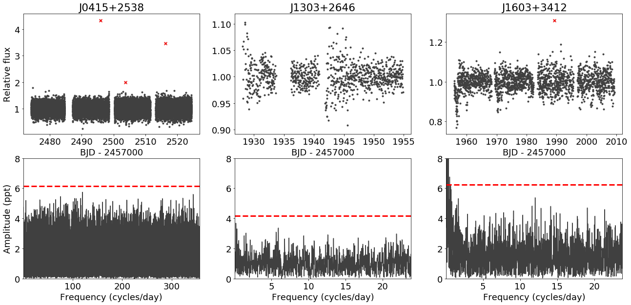
Figure 6: The top panels show the TESS light curves for our three targets as indicated. Points excluded from the analysis are marked by crosses. The bottom panels show the respective Fourier transforms, with the dashed line indicating an adopted detection limit of four times the average amplitude. Aside from low-frequency noise in the periodogram of J1603+3412, no significant peaks appear.

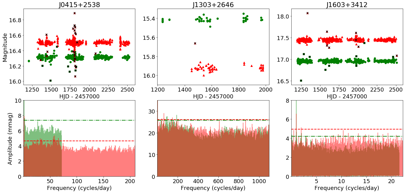
Figure 13: The light curves for the $r$ (red triangles) and $g$ (green circles) filters are shown in the top panel, with excluded datapoints marked by crosses. The bottom panels show the Fourier transform. The only peaks significantly above the detection threshold of four times the average (red dashed line for $r$, green dot-dashed line for $g$) are multiples of one-day aliases, seen clearly in particular for J1603+3412.

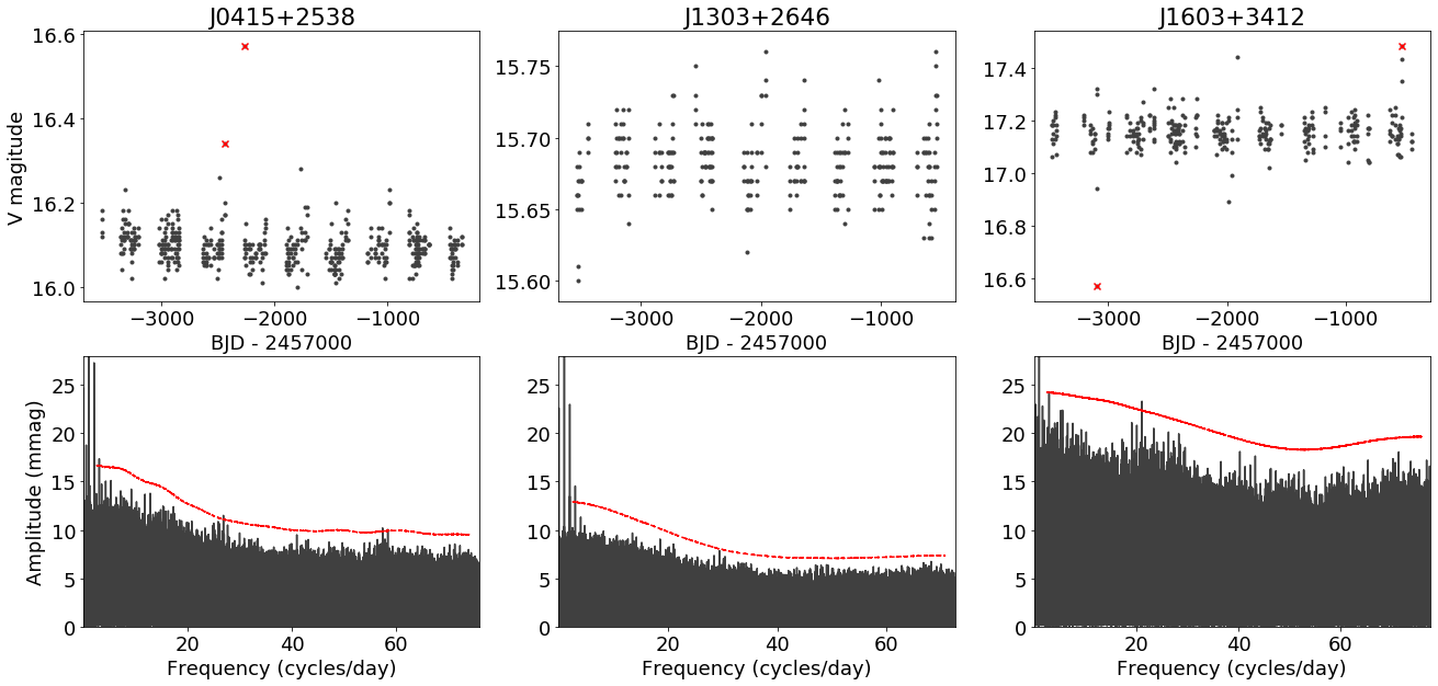
Figure 14: CRTS light curves are shown in the top panels, with the bottom panels showing the respective Fourier transforms. The dashed line indicating the threshold here was calculated as four times the average amplitude in a 5 cycles/day window, given the visible varying amplitude over the frequency spectrum. Multiples of one-day aliases are seen for all light curves. Some other marginal peaks appear slightly above the threshold, but they are not seen in the TESS or ZTF data.

For ZTF and CRTS, we retrieved the light curves from their respective databases for each of our targets. In the case of ZTF, there are two different filters available, $r$ and $g$, and both were retrieved. A Fourier transform was calculated in the same way as for the TESS data, with the Nyquist frequency estimated from the median cadence of observations taken on the same night. Results for ZTF and CRTS are shown in Appendix C (Figs. 13 and 14, respectively).

We do not identify any signs of periodic variability for our targets. The few possibly significant peaks that appear in the Fourier transforms are either multiples of one-day aliases, given the nightly observations of ZTF and CRTS, or appear marginally above the threshold only for one survey and not the others. We can rule out periodic variability in the range of a few minutes to $\approx 600$ days down to an amplitude of 0.6 per cent for J0415+2538 based on the TESS and ZTF light curves, and even longer periods of up to $\approx 1000$ days are ruled out by CRTS down to $\approx 1.5$ per cent. For J1303+2646, TESS rules out periods between an hour and 13 days with amplitudes larger than $\approx 0.4$ per cent, whereas CRTS rules out periods up to $\approx 1000$ days down to $\approx 1.2$ per cent (the ZTF light curve is in turn quite scarce for this object). Finally, for J1603+3412, TESS and ZTF rule out periods between an hour and $\approx 600$ days down to $\approx 0.5$ per cent, whereas the CRTS light curve is not particularly constraining given that the magnitude of the target is near the CRTS detection limit.

4 Discussion

4.1 The detection of magnetic fields in hot subdwarfs

Our three new detections increase the number of hot subdwarfs with confirmed magnetic fields from one to four. Considering that there are 2036 hot subdwarfs identified from SDSS spectra (Geier, 2020), and assuming that there is no bias in selecting magnetic systems (which is reasonable since their colours do not seem to be strongly affected), the three detections from SDSS spectra imply a lower limit to the magnetic fraction of hot subdwarfs of $0.147^{+0.143}_{-0.047}$ per cent. Given the low-resolution of SDSS ($R\approx 2000$), only field strengths larger than $\sim 200$ kG can be identified from visual inspection, implying that lower fields would remain undetected. This detection limit is significantly improved for high resolution ($R\approx 20000$), which would reveal fields down to $\sim 50$ kG. However, high resolution spectra are available for a smaller number of stars ($\approx 200$) which are not homogeneously selected.

Previous searches for magnetic fields in hot subdwarfs mainly used low-resolution spectropolarimetry (Landstreet et al., 2012; Mathys et al., 2012), which has the advantage of lower detection limits of the order of a few hundred gauss to kilogauss, but the disadvantage of requiring the targets to be fairly bright. These searches targeted forty stars of quite different spectral types in various stages of stellar evolution, including sdB stars in close binary systems with white dwarfs as well as low-mass main sequence companions (see Appendix D). Most observations were carried out with the FORS spectropolarimeter at the ESO VLT. Landstreet et al. (2012) and Bagnulo et al. (2012) reanalysed most FORS observations of hot subdwarfs and found no detections even at 2$\sigma$ level, concluding that there is “no evidence for the presence of magnetic fields at the level of 1 kG”.

There are five He-sdOs that have been probed by spectropolarimetry, two eHe-sdO stars and three iHe-sdO stars. Landstreet et al. (2012) derived a mean $B_{z}=90\pm 140$ G for the eHe-sdO CD-31 4800 and $B_{z}=232\pm 178$ G for the iHe-sdO HD 127493. Randall et al. (2015) reported an upper 3 $\sigma$ limit of 300 G for a magnetic field of the iHe star LS IV$-$14 116. Hence, no magnetic fields at a level of a few hundred gauss are present in these three He-sdOs. Earlier work by Elkin (1996) targeted the eHe-sdO star BD$+$25 4655 and the iHe-sdO BD$+$75 325. They measured circularly polarised spectra using the 6-metre telescope at the Russian Academy of Sciences Special Astronomical Observatory and determined a magnetic field strength of $B_{z}=1680\pm 60$ G in BD+75 325. Three additional measurements of BD+75 325 pointed at a variable field strength (Elkin, 1998). In addition, Elkin (1998) failed to detect a magnetic field at the 400 G level from three observations of BD+25 4655. Hence, BD+75 325 would be the only hot subdwarf with a detected magnetic field of a few kG. However, Landstreet et al. (2012) argue that the real uncertainties in these measurements are likely of the order of 1 kG, i.e. of the same order of the reported fields, hence confirmation would be needed with more sensitive methods. In summary, the fields of the four confirmed magnetic He-sdOs are larger by a factor of at least a thousand than those of the few probed He-sdOs.

We compare the location of all subdwarfs probed for magnetic fields in the Kiel diagram with the four magnetic He-sdOs in Fig. 7. The binary status of the stars, inferred from $v_{\mathrm{rad}}$ variability, is also indicated, as well as the He-enrichment. About 60 per cent of the previously studied stars with sufficient $v_{\mathrm{rad}}$ measurements show no evidence of a binary companion, like the known magnetic systems. Strikingly, the four stars for which magnetic fields have been detected cluster very closely together in the Kiel diagram, and none of the previously probed stars are found in this region. This might suggest that a very specific formation scenario is required to generate a magnetic field. However, spectropolarimetric searches in a larger number of stars would be required to confirm that magnetism does not occur for hot subdwarfs in other regions of the Kiel diagram.

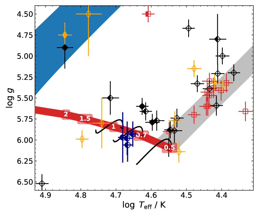
Figure 7: Kiel diagram showing hot subdwarf stars in which magnetic fields have been probed for. The four known magnetic He-sdOs are shown as blue circles. Black diamonds mark apparently single (non-$v_{\mathrm{rad}}$ variable) stars, red squares show known close binaries with white dwarf or low-mass main sequence/brown dwarf companions ($v_{\mathrm{rad}}$ variable), and orange thin diamonds indicate unknown $v_{\mathrm{rad}}$ variability. Helium-poor stars are marked by open symbols, extremely He-rich stars by filled symbols, and intermediately He-rich stars by half filled, half open symbols. For details on the objects, see Appendix D and Table 7. The solid black lines indicate the core helium burning phase in the merger tracks of Yu et al. (2021) for a metallicity of $Z=0.01$ and remnant masses of 0.45, 0.65, 0.85 $M_{\odot}$. The grey shaded region marks the location of the EHB by Dorman et al. (1993) for solar metallicity, the blue shaded region marks the range of post-asymptotic giant branch (AGB) tracks of Miller Bertolami (2016), and thick red line indicates the zero age helium main sequence from Paczyński (1971).

4.2 Formation scenarios for magnetic hot subdwarfs

Interestingly, all four known magnetic systems are of He-sdO spectral type and show remarkably similar atmospheric parameters (see Table 4). This strongly suggests that all four stars were formed by the same evolutionary channel. Dorsch et al. (2022) argued that J0809-2627 is likely the result of a merger, given the derived atmospheric parameters and metal abundances. The lack of radial velocity variability for the three stars presented here provides further evidence for a merger origin for magnetic He-sdOs, taking into account that hot subdwarfs are not expected to form without binary interaction (Pelisoli et al., 2020). Indeed, evidence is increasing that the majority of He-rich sdO stars result from mergers. While the fraction of hydrogen-rich subdwarfs in close binaries is high (about 50 per cent, Maxted et al., 2001; Napiwotzki et al., 2004), Geier et al. (2022) showed that radial velocity variables are very rare amongst He-sdOs, concluding that they are likely formed by mergers.

Other He-rich hot subdwarfs likely formed by mergers were observed by the SPY survey (Napiwotzki et al., 2003; Lisker et al., 2005; Stroeer et al., 2007; Hirsch, 2009), which obtained high resolution spectra ($R\approx 20000$) of tens of hot subwarfs. More recent spectral analyses of He-rich sdO stars from high resolution spectroscopy have been reported by Schindewolf et al. (2018), Naslim et al. (2013); Naslim et al. (2020), Dorsch et al. (2019), and Jeffery et al. (2021) while Latour et al. (2018) analysed four He-poor sdOs. In addition, for well over a hundred sdB stars, spectroscopic analyses based on even higher resolution spectroscopy are available (e.g. Edelmann et al., 2005; Geier et al., 2013; Schneider et al., 2018), but no hint for Zeeman broadening has been found in any of them. Finally, Werner et al. (2022) recently found a CO-rich subtype of He-sdOs whose origin has been attributed to mergers (Miller Bertolami et al., 2022) which also display no Zeeman splitting. This implies that the magnetic fields in the other analysed stars, if existent, must be much weaker than observed for the four magnetic He-sdOs.

We compare the four magnetic subdwarfs to the He-rich subdwarfs from the SPY project and other detailed high-resolution studies (Lanz et al., 1997; Schindewolf et al., 2018; Dorsch et al., 2019; Dorsch et al., 2020; Dorsch, 2022), as well as the CO He-sdOs of Werner et al. (2022) in the Kiel diagram (Fig. 8). The three main subtypes (N-rich, C-rich, C&N-rich) form two distinct clusters, with the N-rich stars being cooler than the C and C&N-rich. The two CO-He-sdOs, the three N-poor eHe-sdOs and the four magnetic iHe-sdOs are amongst the hottest He-sdOs. Though it can be noted that the four magnetic He-sdOs are fairly isolated, it is puzzling that no He-sdO stars other than the four ones discussed here have been found to be magnetic, if mergers were to always lead to magnetic fields. This suggests that some fine-tuning is required in the formation of magnetic systems.

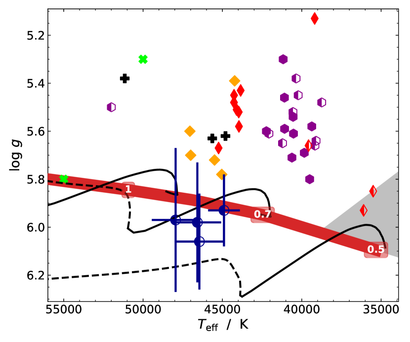
Figure 8: Distribution of He-rich hot subdwarf stars in the Kiel diagram. The blue circles with error bars are the magnetic He-sdOs. Extremely He-rich stars are marked by filled symbols and intermediately He-rich stars by half filled, half open symbols. Surface metal abundances are indicated by purple hexagons (N-rich), red thin diamonds (C&N-rich), orange diamonds (C-rich), or black pluses (C-rich, N-poor). The CO-rich He-sdOs from Werner et al. (2022) are green cross-marks. Merger tracks from Yu et al. (2021) for a metallicity of $Z=0.01$ and remnant masses of 0.45, 0.65, 0.85 $M_{\odot}$ are shown as black lines, where solid lines correspond to the core helium burning phase and dashed lines indicate helium shell burning. The zero age helium main sequence from Paczyński (1971) is shown as a thick red line. The grey shaded region marks the approximate location of the EHB.

Proposed merger scenarios that could form magnetic hot subdwarfs are the merger of two He-core white dwarfs (Han et al., 2003; Zhang & Jeffery, 2012; Yu et al., 2021), the merger between a hybrid CO/He-core white dwarf and a He-core white dwarf (Justham et al., 2011), and the merger between a He-core white dwarf and a low mass CO-core white dwarf (Miller Bertolami et al., 2022). One of the differences between these channels is the resulting mass: the models of Han et al. (2003) and (Miller Bertolami et al., 2022) can only account for masses up to $\approx 0.8$ M_☉, whereas larger masses could be explained by the hybrid merger channel, though the predicted luminosities are higher than those observed for the magnetic He-sdOs. Unfortunately we cannot constrain masses for the studied objects, but future higher-resolution observations and improved astrometry could allow mass estimates to help differentiate between the possible scenarios.

The observed atmospheric abundances can also provide important constraints for the merger models. The rapid mass transfer in He-core white dwarf mergers is predicted to lead to two components (Zhang & Jeffery, 2012): a fast accretion event producing a corona around the primary, which is hot enough for helium burning to occur and to produce carbon and convert nitrogen to neon, and a disc from which the material is slowly accreted onto the surface of the primary. The disc is not hot enough to ignite helium burning. Therefore, the composition of the accreted matter is that of the former He-core white dwarf companion, which is He- and N-rich, but C-poor. Composite merger models assume that both components are created in different relative mass fractions. Accordingly, evolutionary calculations of Zhang & Jeffery (2012) predict that C-rich, N-poor surfaces result from fast hot mergers, N-rich surfaces from slow cold mergers and C&N-rich surfaces from composite models. These variants of the He-core white dwarf merger scenario can explain the different subclasses of He-sdO by the relative mass fraction contained in the corona as opposed to the accretion disc. Expanding on the work of Zhang & Jeffery (2012), Yu et al. (2021) found that the masses of the merging white dwarfs also play a role, with lower masses forming N-rich systems and larger masses leading to C-enrichment. As shown in Fig. 9, the models of Yu et al. (2021) seem to be able to explain the observed $T_{\mathrm{eff}}$ and luminosity of the magnetic He-sdOs. However the exact type of merger cannot be constrained, since we cannot place good constraints on C-enrichment, though N-rich surfaces seem to be a characteristic of the four magnetic iHe-sdOs.

Another puzzle is the division of He-sdOs according to hydrogen content into iHe- and eHe-sdOs as discussed extensively by Luo et al. (2021). All four magnetic He-sdOs show a higher hydrogen abundance than typically observed for He-sdOs (see e.g. Stroeer et al., 2007; Schindewolf et al., 2018). However, neither Yu et al. (2021) nor Justham et al. (2011) have included hydrogen in their models. Model predictions are difficult to make, because the atmosphere corresponds to only a small fraction of the stellar envelope. Attempts have been made by Hall & Jeffery (2016) and Schwab (2018), but, as already pointed out by Dorsch et al. (2022), their models typically predict surfaces poor in hydrogen, at odds with what we find. Yet, we find the stars to lie close to the helium main sequence, which supports that their hydrogen envelopes should be small. The discrepancy between observed and predicted abundances is likely due to limitations on the modelling of the merger, rather than an issue with the idea of a merger itself. For instance, the hydrogen abundance is strongly dependent on rotation, which in turn depends on the angle between the rotation and magnetic axes (García-Berro et al., 2012), which is not included in the models. Our fits to the available observations of the magnetic He-sdOs do not constrain the magnetic field geometry well, as that would require higher-resolution spectra allowing to better resolve the shape of the Zeeman components. The fact that more than one homogeneous component was needed to fit the observed spectra already hints at a non-homogeneous magnetic field.

As for the observed projected rotation velocities, they are typically small in hot subdwarfs, irrespective of their chemical composition (see e.g. Geier & Heber, 2012), and the magnetic systems seem to be no exception, as suggested by our upper limits on $v_{\mathrm{rot}}\sin i$. As an alternative to a precise $v_{\mathrm{rot}}\sin i$ estimate that could constrain rotation, we searched for signs of rotation in publicly available TESS, ZTF, and CRTS light curves for the three stars. However, we find no evidence for periodic variability in any of them. Similarly, the magnetic He-sdO from Dorsch et al. (2022) was also found to show no signs of a rotation period in the light curve. Although magnetism is certainly able to induce stellar spots, it seems that detectable spots are uncommon in the case of strongly magnetic He-sdOs.

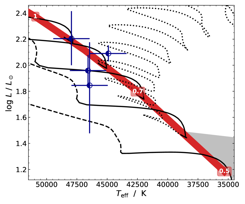
Figure 9: Luminosity as a function of $T_{\mathrm{eff}}$ for the four magnetic He-sdOs (blue half open dots). Merger tracks from Yu et al. (2021) for a metallicity of $Z=0.01$ and remnant masses of 0.85, 0.75, 0.65, 0.55, and 0.45 $M_{\odot}$ are shown in black, where the solid line corresponds to the core helium burning phase and the dashed line indicates helium shell burning. For the 0.55 $M_{\odot}$ track, the pre-helium main sequence phase is shown as a dotted line. The broad red line shows the helium zero-age main sequence from Paczyński (1971), with labelled masses. The grey shaded region marks the approximate location of the EHB.

Apart from mergers, another scenario that could cause magnetism during the hot subdwarf phase is a dynamo acting in the convective core during the main sequence, which has been invoked to explain a fraction of white dwarfs. In this scenario, the field would be exposed when the progenitor star loses its outer layers due to binary interaction. It cannot, however, explain the four known stars given the lack of binary companions. A fossil field from the formation cloud could work similarly, requiring the strongly magnetic Ap and Bp stars to have their cores exposed by binary interaction. The fact that no binary hot subdwarfs have been found to be magnetic could be an argument against these scenarios. The fields in the cores of red giant stars are found to be of the order of $\approx 100$ kG (Fuller et al., 2015), which should be detectable with spectropolarimetry or high-resolution, high signal-to-noise ratio spectra. Only a few tens of hot subdwarfs have spectropolarimetric observations, so the lack of detection in this case is perhaps not surprising. On the other hand, high-resolution spectra are available for hundreds of hot subdwarfs, in particular sdBs. To explain the lack of detection, the fraction of systems with detectable magnetic fields must be a few percent at most, which was also the conclusion of Landstreet et al. (2012).

5 Summary & Conclusions

We identified three new magnetic hot subdwarfs from their SDSS spectra. Using archival WHT/ISIS spectra and SED fits, we estimated their stellar parameters. The observed magnetic fields are in the range $300-500$ kG. Assuming conservation of magnetic flux, this implies fields of the order of $50-150$ MG at the white dwarf stage, consistent with typically observed values (Kepler et al., 2013; Bagnulo & Landstreet, 2021). The similarity between the stellar parameters of all four known magnetic hot subdwarfs points at a common origin for all of them. Their lack of radial velocity variability and observed abundances are consistent with a merger channel, though better data, as well as more complete merger models including hydrogen and magnetic fields, are required to constrain the exact channel. In addition, it seems that a merger alone is not sufficient to trigger a magnetic field, given the lack of detection in high-resolution spectra of likely merger remnants, for example by Napiwotzki et al. (2004) and Werner et al. (2022). Still, our findings provide evidence that mergers are indeed responsible for a fraction of magnetic white dwarfs, in particular those with strong ($\gtrsim 50$ MG) fields.

Formation scenarios other than mergers could lead to magnetism in hot subdwarfs, in particular the stripping of a red giant with a field generated during the main sequence, e.g. due to a convective core. Since evidence of magnetic fields has been found for intermediate-mass red giants ($M\gtrsim 1.1$ M_⊙, Stello et al., 2016), and those can lead to hot subdwarfs with non-canonical masses (i.e. different from the typical $0.47$ M_☉ value resulting from solar-metallicity objects that experience a He-flash), focusing future spectropolarimetric searches on low- or high-mass hot subdwarfs could be profitable. It is worth noting that the stellar-stripping scenario could lead to magnetism also in sdBs – it predicts He-sdOs that are more luminous than the ones observed here, and sdBs that can have similar luminosities but cooler temperature (Götberg et al., 2018).

Finally, we propose that an ‘H’ should be added to the spectral class of magnetic hot subdwarfs showing Zeeman splitting, in analogy to white dwarf classes, making J0415+2538, J1303+2646, J1603+3412, and the prototype J0809-2627 from Dorsch et al. (2022) He-sdOHs.

Data Availability

All the data analysed in this work are public in the respective data archives.

Appendix A Multi-component spectroscopic fits

Table 5: Atmospheric parameters from fits with one, two, or three components to the co-added WHT/ISIS spectra of the three targets.

Star	$T_{\mathrm{eff}}$/K	$\log g$	$\log n(\mathrm{He})/n(\mathrm{H})$	$B_{1}$/kG	$B_{2}$/kG	$B_{3}$/kG	$A_{2}/A_{1}$	$A_{3}/A_{1}$	$\chi^{2}_{r}$
J0415+2538	46730	6.02	$-$0.15	280	–	–	–	–	2.56
J0415+2538	46460	5.95	$-$0.12	266	420	–	0.24	–	2.31
J0415+2538	46430	5.96	$-$0.13	262	377	469	0.21	0.10	2.45
J1303+2646	48880	6.07	+0.22	415	–	–	–	–	2.66
J1303+2646	47920	5.87	+0.32	384	571	–	0.56	–	1.99
J1303+2646	47790	5.84	+0.33	364	584	442	0.67	0.61	1.89
J1603+3412	46620	6.08	+0.06	340	–	–	–	–	2.33
J1603+3412	45980	6.03	+0.05	291	395	–	0.82	–	2.10
J1603+3412	45700	5.95	+0.06	284	377	523	0.90	0.27	2.07

Table 6: The magnetic fields of the individual components and their relative surface ratio for each of the three stars in our best-fit model to the individual WHT/ISIS spectra. The uncertainties for the surface ratios are one sigma statistical, whereas the uncertainties on the magnetic field strengths are estimated systematic uncertainties.

	J0415+2538	J1303+2646	J1603+3412
$B_{1}$ (kG)	$270\pm 15$	$370\pm 20$	$292\pm 15$
$B_{2}$ (kG)	$430\pm 30$	$581\pm 20$	$390\pm 15$
$B_{3}$ (kG)	–	$439\pm 20$	–
$A_{2}/A_{1}$	$0.260^{+0.014}_{-0.014}$	$0.70^{+0.13}_{-0.05}$	$0.81^{+0.16}_{-0.08}$
$A_{3}/A_{1}$	–	$0.56^{+0.23}_{-0.08}$	–

Appendix B SED fits

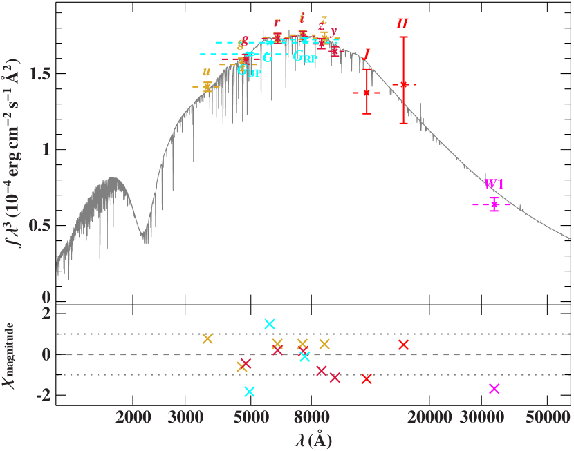
Figure 10: SED fit for J0415+2538. The grey line shows the best-fit, while filter-averaged flux measurements are shown by dashed horizontal lines. Residuals are shown in the bottom panel. The photometric systems are colour-coded: SDSS (ochre, Alam et al., 2015), Pan-STARRS (dark red, Magnier et al., 2020), Gaia EDR3 (cyan, Riello et al., 2021), 2MASS (red, Cutri et al., 2003), and WISE (magenta, Schlafly et al., 2019).

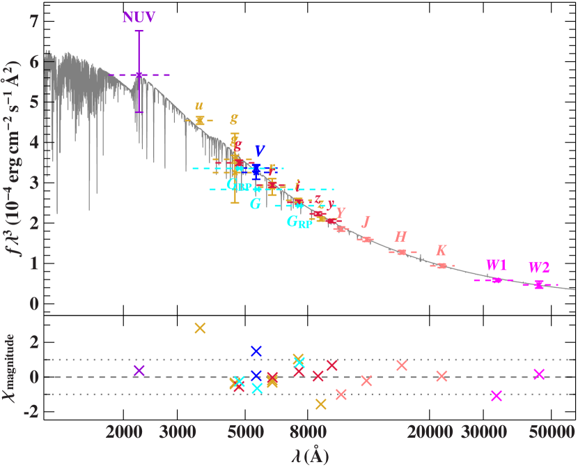
Figure 11: SED fit for J1303+2646. Like for Fig. 10, we show the model in grey and the filter-averaged flux measurements as dashed lines. The photometric systems are GALEX (purple, Bianchi et al., 2017), SDSS (ochre, Alam et al., 2015; Henden et al., 2016), Pan-STARRS (dark red, Magnier et al., 2020), Johnson (blue, Kilkenny et al., 1988; Henden et al., 2016), Gaia EDR3 (cyan, Riello et al., 2021), UKIDSS (pink, Lawrence et al., 2007), and WISE (magenta, Schlafly et al., 2019).

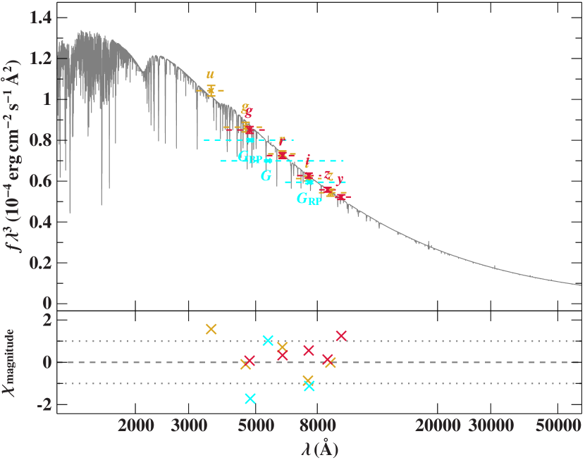
Figure 12: SED fit for J1603+3412 using SDSS (ochre, Alam et al., 2015), Pan-STARRS (dark red, Magnier et al., 2020), and Gaia EDR3 (cyan, Riello et al., 2021).

Appendix C Additional light curves

Appendix D Hot subwarfs probed for magnetic fields

Table 7 lists, to the best of our knowledge, all hot subdwarfs with determined atmospheric parameters that have upper limits or disputed claims of a magnetic field from spectropolarimetry. In addition, they all have spectra of similar quality or better than the stars discussed here, which would reveal Zeeman splitting for fields $\sim 50$ kG or more. Among the hot subdwarfs, the sdB HD 76431 has been studied by spectropolarimitry most extensively (Elkin, 1998; Petit et al., 2012; Landstreet et al., 2012; Chountonov & Geier, 2012) at many epochs, but no detection of a significant magnetic field was reported. Chountonov & Geier (2012) estimated the detection limit at 100–200 G. For other stars in Table 7, no field could be reported at upper detection limits of 1 kG or better (see also Sect. 4.1). For the four sdBs studied by Kawka et al. (2007) the limits turned out to be somewhat higher at several kG. The distribution of the stars listed in Table 7 in the Kiel diagram is shown in Fig. 7. All subtypes are represented (sdB, sdOB, sdO, He-sdB, as well as both variants of He-sdO, that is iHe and eHe-sdOs), though the majority are sdBs. Also some more luminous subdwarfs (e.g. LS IV-12 1, LSE 263, and LSE 153, marked with the prefix “l”) are included which probably evolved from the AGB. HD 188112 is an underluminous sdB of too low mass for core helium burning to ignite, and Balloon 09010 0001 is a large amplitude pulsating (V361Hya) star (Telting et al., 2008). The main types of binaries are also all represented (white dwarf or low-mass companion with short orbital period, main sequence or giant companions in long orbital period systems), with only seven stars lacking sufficient $v_{\mathrm{rad}}$ measurements to allow conclusive remarks about binary status. An unconfirmed detection of a variable magnetic field was reported for BD+75 325 (see Sect. 4.1).

Table 7: Hot subdwarfs with well-determined atmospheric parameters and upper limits on magnetic fields, typically of the order of a few kG. The $v_{\mathrm{rad}}$ variability is inferred from multi-epoch observations indicated in the notes. The orbital period is given in days when determined, and the entry “no” indicates no $v_{\mathrm{rad}}$ variations detected on long time scales ($>$months).

Name	Spectral	$v_{\mathrm{rad}}$	$T_{\mathrm{eff}}$	$\log g$	$\log n(\mathrm{He})/n(\mathrm{H})$	References
	class	variablity				Atmospheric parameters	$B$ limit
BD+75 325	iHe-sdO	nos17	$52000\pm 2000$	$5.50\pm 0.20$	+0.00	Lanz et al. (1997)	Elkin (1996, 1998)
HD 128220	lHe-sdO+GIII	871.78HH	$40600\pm 400$	$4.5\pm 0.1$	$0.30\pm 0.05$	Rauch (1993)	Elkin (1998)
BD+25 4655	eHe-sdO	noE	$39500\pm 1000$	$5.8\pm 0.1$	$1.55\pm 0.15$	Dorsch (2022)	Elkin (1998)
Feige 87	sdB+G	936V	$27270\pm 500$	$5.47\pm 0.15$	$-2.56^{+0.22}_{-0.50}$	Vos et al. (2013)	Elkin (1998)
HD 76431	sdB	noR,Kh,CG	$31180\pm 220$	$4.67\pm 0.03$	$-1.58\pm 0.05$	Khalack et al. (2014)	Chountonov & Geier (2012)
GD 687	sdB+WD	0.37765G	$24350\pm 360$	$5.32\pm 0.05$	$-2.38$	Lisker et al. (2005)	Kawka et al. (2007)
GD 1669	sdB	noGH	$34126\pm 360$	$5.77\pm 0.05$	$-1.36$	Lisker et al. (2005)	Kawka et al. (2007)
GD 108	sdB+?	3.18095C	$27760\pm 670$	$5.60\pm 0.11$	$<-3.0$	Kawka et al. (2007)	Kawka et al. (2007)
WD 1153-484	sdB		$30080\pm 660$	$5.15\pm 0.10$	$<-3.0$	Kawka et al. (2007)	Kawka et al. (2007)
SB 290	sdB+K	uncertainG	$26300\pm 100$	$5.31\pm 0.01$	$-2.52\pm 0.08$	Geier et al. (2013)	Landstreet et al. (2012)
HD 4539	sdB	noS,K,E	$23200\pm 100$	$5.20\pm 0.01$	$-2.27\pm 0.24$	Schneider et al. (2018)	Landstreet et al. (2012)
PHL 932	sdB	noK,E	$33644\pm 500$	$5.74\pm 0.05$	$-1.64\pm 0.05$	Lisker et al. (2005)	Landstreet et al. (2012)
PG 0133+114	sdB+WD	1.23787E	$30073\pm 201$	$5.70\pm 0.04$	$-2.14\pm 0.04$	Luo et al. (2021)	Landstreet et al. (2012)
SB 707	sdB+WD	5.85E	$35400\pm 500$	$5.90\pm 0.05$	$-2.90\pm 0.10$	O’Toole & Heber (2006)	Landstreet et al. (2012)
PG 0342+026	sdB	noE,S	$26000\pm 1100$	$5.59\pm 0.12$	$-2.69\pm 0.10$	Geier et al. (2013)	Landstreet et al. (2012)
HD 127493	iHe-sdO	noE	$42070\pm 180$	$5.61\pm 0.04$	$0.33\pm 0.06$	Dorsch et al. (2019)	Landstreet et al. (2012)
HD 149382	sdB	noJ	$34200\pm 1000$	$5.89\pm 0.15$	$-1.60\pm 0.10$	Saffer et al. (1994)	Landstreet et al. (2012)
HD 171858	sdB+WD	1.63280E	$27200\pm 800$	$5.30\pm 0.10$	$-2.84\pm 0.1$	Geier et al. (2010b)	Landstreet et al. (2012)
HD 188112	sdB+WD	0.6065812E	$21500\pm 500$	$5.66\pm 0.06$	$-5.00$	Heber et al. (2003)	Landstreet et al. (2012)
HD 205805	sdB	noE	$25000\pm 500$	$5.00\pm 0.10$	$-2.00\pm 0.2$	Przybilla et al. (2006)	Landstreet et al. (2012)
JL 87	iHe-sdB	noE	$25800\pm 1000$	$4.80\pm 0.30$	$0.33$	Ahmad et al. (2007)	Landstreet et al. (2012)
$[$CW 83$]$ 0512-08	sdB	noE,S	$38400\pm 1100$	$5.77\pm 0.12$	$-0.73\pm 0.10$	Geier et al. (2013)	Landstreet et al. (2012)
CPD-64 481	sdB+BD?	0.27726315Sch	$27500\pm 500$	$5.60\pm 0.05$	$-2.50\pm 0.10$	O’Toole & Heber (2006)	Landstreet et al. (2012)
CD-31 4800	eHe-sdO	noE	$42230\pm 300$	$5.60\pm 0.1$	$2.61\pm 0.20$	Schindewolf et al. (2018)	Landstreet et al. (2012)
PG 0909+276	sdOB	noE	$35500\pm 500$	$6.09\pm 0.05$	$-1.00\pm 0.10$	Geier et al. (2013)	Landstreet et al. (2012)
LS IV-12 1	lsdO	noE	$60000\pm 5000$	$4.50\pm 0.50$	$-0.95\pm 0.20$	Heber & Hunger (1987)	Landstreet et al. (2012)
LSE 263	lHe-sdO	noK	$70000\pm 2500$	$4.90\pm 0.25$	$>$+1.0	Husfeld et al. (1989)	Landstreet et al. (2012)
LSE 153	lHe-sdO		$70000\pm 1500$	$4.75\pm 0.15$	$>$+1.0	Husfeld et al. (1989)	Landstreet et al. (2012)
BD+28 4211	sdO	noL,H	$81300\pm 1200$	$6.52\pm 0.05$	$-1.12\pm 0.05$	Latour et al. (2015)	Landstreet et al. (2012)
EC 11481-2303	sdO		$55000\pm 5000$	$5.8\pm 0.3$	$-2.0\pm 0.3$	Rauch et al. (2010)	Landstreet et al. (2012)
SB 410	sdB+WD	0.8227E	$27600\pm 500$	$5.43\pm 0.05$	$-2.71\pm 0.10$	Geier et al. (2010b)	Mathys et al. (2012)
SB 459	sdB		$24900\pm 500$	$5.35\pm 0.10$	$-2.58\pm 0.10$	Sahoo et al. (2020)	Mathys et al. (2012)
LB 1516	sdB+WD	10.3598G2	$25200\pm 1100$	$5.41\pm 0.12$	$-2.78\pm 0.10$	Geier et al. (2013)	Mathys et al. (2012)
JL 194	sdB	noE	$25770\pm 380$	$5.21\pm 0.06$	$-2.69\pm 0.06$	Uzundag et al. (2021)	Mathys et al. (2012)
GD 1110	sdB+dM/BD	0.3131Sch	$26500\pm 1100$	$5.38\pm 0.12$	$-2.54\pm 0.10$	Geier et al. (2013)	Mathys et al. (2012)
SB 815	sdB	noK	$27200\pm 550$	$5.39\pm 0.10$	$-2.94\pm 0.01$	Schneider et al. (2018)	Mathys et al. (2012)
Feige 66	sdB		$33220\pm 370$	$6.14\pm 0.08$	$-1.61\pm 0.11$	Lei et al. (2018)	Petit et al. (2012)
LS IV-14 116	iHe-sdO	noJS,Ra	$35500\pm 1000$	$5.85\pm 0.10$	$-0.60\pm 0.10$	Dorsch et al. (2020)	Randall et al. (2015)
Balloon 09010 0001	sdB	0.0041T	$29446\pm 500$	$5.33\pm 0.1$	$-2.54\pm 0.2$	Oreiro et al. (2004)	Savanov et al. (2013)
Feige 34	sdO		$62550\pm 600$	$5.99\pm 0.03$	$-1.79\pm 0.04$	Latour et al. (2018)	Valyavin et al. (2006)

Notes: E = Edelmann et al. (2005) (variables published, non-variables: priv. com.), S17 =Schork (2017), S = Silvotti et al. (2020), J = Jacobs et al. (2011), K = Kawka et al. (2015), Kh = Khalack et al. (2014), R = Ramspeck et al. (2001), Ra = Randall et al. (2015), L = Latour et al. (2015), H = Herbig (1999), JS = Jeffery et al. (2015), R = Randall et al. (2015), C = Copperwheat et al. (2011), G = Geier et al. (2010a), GH = Geier & Heber (2012), T = Telting et al. (2008), HH=Howarth & Heber (1990), CG=Chountonov & Geier (2012), G2=Geier et al. (2014), Sch=Schaffenroth et al. (2014) V=Vos et al. (2013).

References

- Ahmad et al. (2007) Ahmad A., Behara N. T., Jeffery C. S., Sahin T., Woolf V. M., 2007, A&A, 465, 541
- Alam et al. (2015) Alam S., et al., 2015, ApJS, 219, 12
- Aller et al. (2020) Aller A., Lillo-Box J., Jones D., Miranda L. F., Barceló Forteza S., 2020, A&A, 635, A128
- Angel et al. (1981) Angel J. R. P., Borra E. F., Landstreet J. D., 1981, ApJS, 45, 457
- Babcock (1947) Babcock H. W., 1947, ApJ, 105, 105
- Bachulski et al. (2016) Bachulski S., Baran A. S., Jeffery C. S., Østensen R. H., Reed M. D., Telting J. H., Kuutma T., 2016, Acta Astron., 66, 455
- Bagnulo & Landstreet (2021) Bagnulo S., Landstreet J. D., 2021, MNRAS, 507, 5902
- Bagnulo et al. (2012) Bagnulo S., Landstreet J. D., Fossati L., Kochukhov O., 2012, A&A, 538, A129
- Bagnulo et al. (2015) Bagnulo S., Fossati L., Landstreet J. D., Izzo C., 2015, A&A, 583, A115
- Balona et al. (2019) Balona L. A., et al., 2019, MNRAS, 485, 3457
- Bellm et al. (2019) Bellm E. C., et al., 2019, PASP, 131, 018002
- Bianchi et al. (2017) Bianchi L., Shiao B., Thilker D., 2017, ApJS, 230, 24
- Briggs et al. (2015) Briggs G. P., Ferrario L., Tout C. A., Wickramasinghe D. T., Hurley J. R., 2015, MNRAS, 447, 1713
- Briggs et al. (2018) Briggs G. P., Ferrario L., Tout C. A., Wickramasinghe D. T., 2018, MNRAS, 478, 899
- Charpinet et al. (2018) Charpinet S., Giammichele N., Zong W., Van Grootel V., Brassard P., Fontaine G., 2018, Open Astronomy, 27, 112
- Chountonov & Geier (2012) Chountonov G., Geier S., 2012, in Kilkenny D., Jeffery C. S., Koen C., eds, Astronomical Society of the Pacific Conference Series Vol. 452, Fifth Meeting on Hot Subdwarf Stars and Related Objects. p. 93 (arXiv:1112.2921)
- Copperwheat et al. (2011) Copperwheat C. M., Morales-Rueda L., Marsh T. R., Maxted P. F. L., Heber U., 2011, MNRAS, 415, 1381
- Culpan et al. (2022) Culpan R., Geier S., Reindl N., Pelisoli I., Gentile-Fusillo N., Vorontseva A., 2022, A&A, in press
- Cutri et al. (2003) Cutri R. M., et al., 2003, VizieR Online Data Catalog, p. II/246
- Dorman et al. (1993) Dorman B., Rood R. T., O’Connell R. W., 1993, ApJ, 419, 596
- Dorsch (2022) Dorsch M., 2022, PhD thesis, Friedrich-Alexander University Erlangen-Nürnberg, in prep.
- Dorsch et al. (2019) Dorsch M., Latour M., Heber U., 2019, A&A, 630, A130
- Dorsch et al. (2020) Dorsch M., Latour M., Heber U., Irrgang A., Charpinet S., Jeffery C. S., 2020, A&A, 643, A22
- Dorsch et al. (2022) Dorsch M., Reindl N., Pelisoli I., Heber U., Geier S., Istrate A. G., Justham S., 2022, arXiv e-prints, p. arXiv:2201.08146
- Drake et al. (2009) Drake A. J., et al., 2009, ApJ, 696, 870
- Edelmann et al. (2005) Edelmann H., Heber U., Altmann M., Karl C., Lisker T., 2005, A&A, 442, 1023
- Eisenstein et al. (2011) Eisenstein D. J., et al., 2011, AJ, 142, 72
- El-Badry et al. (2021) El-Badry K., Rix H.-W., Heintz T. M., 2021, MNRAS, 506, 2269
- Elkin (1996) Elkin V. G., 1996, A&A, 312, L5
- Elkin (1998) Elkin V. G., 1998, Contributions of the Astronomical Observatory Skalnate Pleso, 27, 452
- Feinstein et al. (2019) Feinstein A. D., et al., 2019, PASP, 131, 094502
- Ferrario et al. (2009) Ferrario L., Pringle J. E., Tout C. A., Wickramasinghe D. T., 2009, MNRAS, 400, L71
- Ferrario et al. (2015) Ferrario L., de Martino D., Gänsicke B. T., 2015, Space Sci. Rev., 191, 111
- Fitzpatrick et al. (2019) Fitzpatrick E. L., Massa D., Gordon K. D., Bohlin R., Clayton G. C., 2019, ApJ, 886, 108
- Fuller et al. (2015) Fuller J., Cantiello M., Stello D., Garcia R. A., Bildsten L., 2015, Science, 350, 423
- Gaia Collaboration et al. (2016) Gaia Collaboration et al., 2016, A&A, 595, A1
- Gaia Collaboration et al. (2021) Gaia Collaboration et al., 2021, A&A, 649, A1
- García-Berro et al. (2012) García-Berro E., et al., 2012, ApJ, 749, 25
- Geier (2020) Geier S., 2020, A&A, 635, A193
- Geier & Heber (2012) Geier S., Heber U., 2012, A&A, 543, A149
- Geier et al. (2010a) Geier S., Heber U., Kupfer T., Napiwotzki R., 2010a, A&A, 515, A37
- Geier et al. (2010b) Geier S., Heber U., Podsiadlowski P., Edelmann H., Napiwotzki R., Kupfer T., Müller S., 2010b, A&A, 519, A25
- Geier et al. (2013) Geier S., Heber U., Edelmann H., Morales-Rueda L., Kilkenny D., O’Donoghue D., Marsh T. R., Copperwheat C., 2013, A&A, 557, A122
- Geier et al. (2014) Geier S., et al., 2014, A&A, 562, A95
- Geier et al. (2015) Geier S., et al., 2015, A&A, 577, A26
- Geier et al. (2022) Geier S., Dorsch M., Pelisoli I., Reindl N., Heber U., Irrgang A., 2022, arXiv e-prints, p. arXiv:2202.09608
- Götberg et al. (2018) Götberg Y., de Mink S. E., Groh J. H., Kupfer T., Crowther P. A., Zapartas E., Renzo M., 2018, A&A, 615, A78
- Hall & Jeffery (2016) Hall P. D., Jeffery C. S., 2016, MNRAS, 463, 2756
- Han et al. (2002) Han Z., Podsiadlowski P., Maxted P. F. L., Marsh T. R., Ivanova N., 2002, MNRAS, 336, 449
- Han et al. (2003) Han Z., Podsiadlowski P., Maxted P. F. L., Marsh T. R., 2003, MNRAS, 341, 669
- Heber (2016) Heber U., 2016, PASP, 128, 082001
- Heber & Hunger (1987) Heber U., Hunger K., 1987, The Messenger, 47, 36
- Heber et al. (2003) Heber U., Edelmann H., Lisker T., Napiwotzki R., 2003, A&A, 411, L477
- Heber et al. (2013) Heber U., Geier S., Gaensicke B., 2013, in European Physical Journal Web of Conferences. p. 04002 (arXiv:1211.5315), doi:10.1051/epjconf/20134304002
- Henden et al. (2016) Henden A. A., Templeton M., Terrell D., Smith T. C., Levine S., Welch D., 2016, VizieR Online Data Catalog, p. II/336
- Herbig (1999) Herbig G. H., 1999, PASP, 111, 1144
- Hirsch (2009) Hirsch H. A., 2009, PhD thesis, Friedrich-Alexander University Erlangen-Nürnberg
- Howarth & Heber (1990) Howarth I. D., Heber U., 1990, PASP, 102, 912
- Hubeny & Lanz (2017c) Hubeny I., Lanz T., 2017c, preprint, (arXiv:1706.01859)
- Hubeny & Lanz (2017a) Hubeny I., Lanz T., 2017a, preprint, (arXiv:1706.01935)
- Hubeny & Lanz (2017b) Hubeny I., Lanz T., 2017b, preprint, (arXiv:1706.01937)
- Husfeld et al. (1989) Husfeld D., Butler K., Heber U., Drilling J. S., 1989, A&A, 222, 150
- Isern et al. (2017) Isern J., García-Berro E., Külebi B., Lorén-Aguilar P., 2017, ApJ, 836, L28
- Jacobs et al. (2011) Jacobs V. A., et al., 2011, in Schuh S., Drechsel H., Heber U., eds, American Institute of Physics Conference Series Vol. 1331, Planetary Systems Beyond the Main Sequence. pp 304–309 (arXiv:1101.4158), doi:10.1063/1.3556216
- Jeffery et al. (2013) Jeffery C. S., et al., 2013, MNRAS, 429, 3207
- Jeffery et al. (2015) Jeffery C. S., Ahmad A., Naslim N., Kerzendorf W., 2015, MNRAS, 446, 1889
- Jeffery et al. (2021) Jeffery C. S., Miszalski B., Snowdon E., 2021, MNRAS, 501, 623
- Justham et al. (2011) Justham S., Podsiadlowski P., Han Z., 2011, MNRAS, 410, 984
- Kawka et al. (2007) Kawka A., Vennes S., Schmidt G. D., Wickramasinghe D. T., Koch R., 2007, ApJ, 654, 499
- Kawka et al. (2015) Kawka A., Vennes S., O’Toole S., Németh P., Burton D., Kotze E., Buckley D. A. H., 2015, MNRAS, 450, 3514
- Kemp et al. (1970) Kemp J. C., Swedlund J. B., Landstreet J. D., Angel J. R. P., 1970, ApJ, 161, L77
- Kepler et al. (2013) Kepler S. O., et al., 2013, MNRAS, 429, 2934
- Khalack et al. (2014) Khalack V., Yameogo B., LeBlanc F., Fontaine G., Green E., Van Grootel V., Petit P., 2014, MNRAS, 445, 4086
- Kilkenny et al. (1988) Kilkenny D., Heber U., Drilling J. S., 1988, South African Astronomical Observatory Circular, 12, 1
- Lallement et al. (2018) Lallement R., et al., 2018, A&A, 616, A132
- Landstreet (1967) Landstreet J. D., 1967, Physical Review, 153, 1372
- Landstreet et al. (2012) Landstreet J. D., Bagnulo S., Fossati L., Jordan S., O’Toole S. J., 2012, A&A, 541, A100
- Lanz et al. (1997) Lanz T., Hubeny I., Heap S. R., 1997, ApJ, 485, 843
- Latour et al. (2015) Latour M., Fontaine G., Green E. M., Brassard P., 2015, A&A, 579, A39
- Latour et al. (2018) Latour M., Chayer P., Green E. M., Irrgang A., Fontaine G., 2018, A&A, 609, A89
- Lawrence et al. (2007) Lawrence A., et al., 2007, MNRAS, 379, 1599
- Lei et al. (2018) Lei Z., Zhao J., Németh P., Zhao G., 2018, ApJ, 868, 70
- Lindegren et al. (2021) Lindegren L., et al., 2021, A&A, 649, A4
- Lisker et al. (2005) Lisker T., Heber U., Napiwotzki R., Christlieb N., Han Z., Homeier D., Reimers D., 2005, A&A, 430, 223
- Luo et al. (2021) Luo Y., Németh P., Wang K., Wang X., Han Z., 2021, ApJS, 256, 28
- Magnier et al. (2020) Magnier E. A., et al., 2020, ApJS, 251, 6
- Marsh (1989) Marsh T. R., 1989, PASP, 101, 1032
- Mathys et al. (2012) Mathys G., Hubrig S., Mason E., Michaud G., Schöller M., Wesemael F., 2012, Astronomische Nachrichten, 333, 30
- Maxted et al. (2001) Maxted P. F. L., Heber U., Marsh T. R., North R. C., 2001, MNRAS, 326, 1391
- Miller Bertolami (2016) Miller Bertolami M. M., 2016, A&A, 588, A25
- Miller Bertolami et al. (2022) Miller Bertolami M. M., Battich T., Córsico A. H., Althaus L. G., Wachlin F. C., 2022, arXiv e-prints, p. arXiv:2202.05635
- Momany et al. (2020) Momany Y., et al., 2020, Nature Astronomy, 4, 1092
- Moss (2001) Moss D., 2001, in Mathys G., Solanki S. K., Wickramasinghe D. T., eds, Astronomical Society of the Pacific Conference Series Vol. 248, Magnetic Fields Across the Hertzsprung-Russell Diagram. p. 305
- Napiwotzki et al. (2003) Napiwotzki R., et al., 2003, The Messenger, 112, 25
- Napiwotzki et al. (2004) Napiwotzki R., Karl C. A., Lisker T., Heber U., Christlieb N., Reimers D., Nelemans G., Homeier D., 2004, Ap&SS, 291, 321
- Naslim et al. (2013) Naslim N., Jeffery C. S., Hibbert A., Behara N. T., 2013, MNRAS, 434, 1920
- Naslim et al. (2020) Naslim N., Jeffery C. S., Woolf V. M., 2020, MNRAS, 491, 874
- O’Toole & Heber (2006) O’Toole S. J., Heber U., 2006, A&A, 452, 579
- Oreiro et al. (2004) Oreiro R., Ulla A., Pérez Hernández F., Østensen R., Rodríguez López C., MacDonald J., 2004, A&A, 418, 243
- Paczyński (1971) Paczyński B., 1971, Acta Astron., 21, 1
- Pelisoli et al. (2020) Pelisoli I., Vos J., Geier S., Schaffenroth V., Baran A. S., 2020, A&A, 642, A180
- Petit et al. (2012) Petit P., Van Grootel V., Bagnulo S., Charpinet S., Wade G. A., Green E. M., 2012, in Kilkenny D., Jeffery C. S., Koen C., eds, Astronomical Society of the Pacific Conference Series Vol. 452, Fifth Meeting on Hot Subdwarf Stars and Related Objects. p. 87 (arXiv:1110.5227)
- Przybilla et al. (2006) Przybilla N., Nieva M. F., Edelmann H., 2006, Baltic Astronomy, 15, 107
- Ramspeck et al. (2001) Ramspeck M., Heber U., Edelmann H., 2001, A&A, 379, 235
- Randall et al. (2015) Randall S. K., Bagnulo S., Ziegerer E., Geier S., Fontaine G., 2015, A&A, 576, A65
- Rauch (1993) Rauch T., 1993, A&A, 276, 171
- Rauch et al. (2010) Rauch T., Werner K., Kruk J. W., 2010, Ap&SS, 329, 133
- Reed et al. (2014) Reed M. D., Foster H., Telting J. H., Østensen R. H., Farris L. H., Oreiro R., Baran A. S., 2014, MNRAS, 440, 3809
- Reed et al. (2018) Reed M. D., et al., 2018, Open Astronomy, 27, 157
- Reindl et al. (2019) Reindl N., et al., 2019, MNRAS, 482, L93
- Ricker et al. (2015) Ricker G. R., et al., 2015, Journal of Astronomical Telescopes, Instruments, and Systems, 1, 014003
- Riello et al. (2021) Riello M., et al., 2021, A&A, 649, A3
- Saffer et al. (1994) Saffer R. A., Bergeron P., Koester D., Liebert J., 1994, ApJ, 432, 351
- Sahoo et al. (2020) Sahoo S. K., et al., 2020, MNRAS, 495, 2844
- Savanov et al. (2013) Savanov I. S., Romaniuk I. I., Semenko E. A., Dmitrienko E. S., 2013, Astronomy Reports, 57, 751
- Schaffenroth et al. (2014) Schaffenroth V., Classen L., Nagel K., Geier S., Koen C., Heber U., Edelmann H., 2014, A&A, 570, A70
- Schindewolf et al. (2018) Schindewolf M., Németh P., Heber U., Battich T., Miller Bertolami M. M., Irrgang A., Latour M., 2018, A&A, 620, A36
- Schlafly et al. (2019) Schlafly E. F., Meisner A. M., Green G. M., 2019, ApJS, 240, 30
- Schneider et al. (2016) Schneider F. R. N., Podsiadlowski P., Langer N., Castro N., Fossati L., 2016, MNRAS, 457, 2355
- Schneider et al. (2018) Schneider D., Irrgang A., Heber U., Nieva M. F., Przybilla N., 2018, A&A, 618, A86
- Schneider et al. (2019) Schneider F. R. N., Ohlmann S. T., Podsiadlowski P., Röpke F. K., Balbus S. A., Pakmor R., Springel V., 2019, Nature, 574, 211
- Schork (2017) Schork M., 2017, Teacher’s thesis, Friedrich-Alexander University Erlangen-Nürnberg
- Schwab (2018) Schwab J., 2018, MNRAS, 476, 5303
- Silvotti et al. (2020) Silvotti R., Ostensen R. H., Telting J. H., 2020, arXiv e-prints, p. arXiv:2002.04545
- Stello et al. (2016) Stello D., Cantiello M., Fuller J., Huber D., García R. A., Bedding T. R., Bildsten L., Silva Aguirre V., 2016, Nature, 529, 364
- Stroeer et al. (2007) Stroeer A., Heber U., Lisker T., Napiwotzki R., Dreizler S., Christlieb N., Reimers D., 2007, A&A, 462, 269
- Telting et al. (2008) Telting J. H., Geier S., Østensen R. H., Heber U., Glowienka L., Nielsen T., Oreiro R., Frandsen S., 2008, A&A, 492, 815
- Tout et al. (2008) Tout C. A., Wickramasinghe D. T., Liebert J., Ferrario L., Pringle J. E., 2008, MNRAS, 387, 897
- Uzundag et al. (2021) Uzundag M., et al., 2021, A&A, 651, A121
- Valyavin & Fabrika (1999) Valyavin G., Fabrika S., 1999, in Solheim S. E., Meistas E. G., eds, Astronomical Society of the Pacific Conference Series Vol. 169, 11th European Workshop on White Dwarfs. p. 206
- Valyavin et al. (2006) Valyavin G., Bagnulo S., Fabrika S., Reisenegger A., Wade G. A., Han I., Monin D., 2006, ApJ, 648, 559
- Vos et al. (2013) Vos J., Østensen R. H., Németh P., Green E. M., Heber U., Van Winckel H., 2013, A&A, 559, A54
- Vos et al. (2019) Vos J., Vučković M., Chen X., Han Z., Boudreaux T., Barlow B. N., Østensen R., Németh P., 2019, MNRAS, 482, 4592
- Vos et al. (2021) Vos J., et al., 2021, A&A, 655, A43
- Werner et al. (1995) Werner K., Dreizler S., Heber U., Rauch T., Wisotzki L., Hagen H. J., 1995, A&A, 293, L75
- Werner et al. (2022) Werner K., Reindl N., Geier S., Pritzkuleit M., 2022, MNRAS, 511, L66
- Woltjer (1964) Woltjer L., 1964, ApJ, 140, 1309
- Wurster et al. (2018) Wurster J., Bate M. R., Price D. J., 2018, MNRAS, 481, 2450
- Yu et al. (2021) Yu J., Zhang X., Lü G., 2021, MNRAS, 504, 2670
- Zhang & Jeffery (2012) Zhang X., Jeffery C. S., 2012, MNRAS, 419, 452