Gravitational Bremsstrahlung with tidal effects
in the post-Minkowskian expansion

Abstract

We compute the mass and current quadrupole tidal corrections to the four-momentum and energy flux radiated during the scattering of two spinless bodies, at leading order in $G$ and at all orders in the velocities, using the effective field theory worldline approach. In particular, we derive the conserved stress-energy tensor linearly coupled to gravity generated by the two bodies, including tidal fields, and the waveform in direct space. The integral is solved using scattering amplitude techniques. We show that our expressions are consistent with existing results up to the next-to-next-to-leading order in the post-Newtonian expansion.

Introduction – The direct detection of gravitational waves from binary black holes Abbott:2016blz and neutron stars TheLIGOScientific:2017qsa has opened an new way to test gravity in the strong-field regime Berti:2015itd and explore fundamental physics Barausse:2020rsu . An important target of current and future observations is the measurement of tidal deformations during the coalescence of compact objects Damour:1992qi ; Damour:1993zn ; Goldberger:2005cd ; Hinderer:2007mb ; Flanagan:2007ix ; Damour:2009vw ; Binnington:2009bb ; Hinderer:2009ca ; Kol:2011vg ; Damour:2012yf ; Favata:2013rwa , which may shed light on the internal structure of neutron stars Baiotti:2016qnr , the nature of black holes Barack:2018yly or the existence of more exotic astrophysical objects Buonanno:2014aza ; Cardoso:2019rvt ; Baumann:2019ztm .

Tidal deformations affect the conservative two-body dynamics as well as the emitted energy in gravitational waves. They have been studied utilising different analytical techniques, most notably the post-Newtonian (PN) expansion Mora:2003wt ; Vines:2010ca ; Vines:2011ud ; Henry:2019xhg ; Henry:2020pzq ; Henry:2020ski , the effective-one-body approach Damour:2009wj ; Bini:2012gu ; Steinhoff:2016rfi , Non-Relativistic-General-Relativity (NRGR) Goldberger:2004jt ; Goldberger:2007hy ; Foffa:2013qca ; Rothstein:2014sra ; Porto:2016pyg ; Levi:2018nxp and the self-force formalism Bini:2014zxa ; Bini:2018svh ; Bini:2018kov ; Bini:2018dki (see Dietrich:2020eud for a review).

Another technique that has been employed to study the gravitational two-body problem is the post-Minkowskian (PM) method Bertotti:1956pxu ; Bertotti:1960wuq ; Havas:1962zz ; Westpfahl:1979gu ; Portilla:1980uz ; Bel:1981be ; Westpfahl:1985tsl ; Damour:2016gwp ; Damour:2017zjx , consisting in expanding the gravitational dynamics for small interactions, while keeping the velocities fully relativistic. It has been recently subject of great interest and activity, in particular in association with the effective-one-body approach Damour:2016gwp ; Damour:2017zjx ; Bini:2017xzy ; Bini:2018ywr ; Vines:2018gqi ; Damour:2019lcq ; Antonelli:2019ytb , scattering amplitude techniques Neill:2013wsa ; Bjerrum-Bohr:2013bxa ; Luna:2017dtq ; Bjerrum-Bohr:2018xdl ; Kosower:2018adc ; Cheung:2018wkq ; Bern:2019nnu ; Bern:2019crd ; Cristofoli:2019neg ; Cristofoli:2020uzm ; Cheung:2020gyp ; Bern:2020buy ; Bern:2021dqo ; Bern:2021yeh ; DiVecchia:2021bdo ; Bjerrum-Bohr:2021vuf ; Bjerrum-Bohr:2021din ; Damgaard:2021ipf , and worldline approaches Foffa:2013gja ; Goldberger:2016iau ; Goldberger:2017vcg ; Kalin:2020mvi ; Kalin:2020fhe ; Loebbert:2020aos ; Mogull:2020sak ; Liu:2021zxr ; Cho:2021mqw ; Dlapa:2021npj ; Dlapa:2021vgp ; Jakobsen:2021lvp ; Jakobsen:2021zvh ; Cho:2022syn ; Jakobsen:2022fcj . Tidal effects have been studied with the PM expansion in Bern:2020uwk ; Cheung:2020sdj ; AccettulliHuber:2020oou ; Haddad:2020que ; Aoude:2020onz ; Bini:2020flp ; Kalin:2020lmz ; Cheung:2020gbf ; Huber:2020xny ; Goldberger:2019xef ; Goldberger:2020wbx ; Goldberger:2020fot . These developments concern the scattering of two bodies moving on unbounded orbits but computed observables can be extended to the case of bound orbits by applying the so-called “boundary-to-bound” (B2B) dictionary, consisting in an analytic continuation between hyperbolic and elliptic motion Kalin:2019rwq ; Kalin:2019inp ; Bini:2020hmy ; Cho:2021arx .

A long-standing and, until recently, unsolved problem was the calculation of the four-momentum radiated in gravitational waves—the so-called gravitational Bremsstrahlung—during the scattering of two spinless bodies, at leading PM order, i.e. at ${\cal O}(G^{3})$. This was finally obtained very recently in Herrmann:2021lqe ; Herrmann:2021tct via the amplitude-based method of Kosower:2018adc , in DiVecchia:2021bdo using the eikonal approach and in Riva:2021vnj by a classical effective field theory (EFT) worldline approach. (See also Amati:1990xe ; DiVecchia:2019myk ; DiVecchia:2019kta ; Bern:2020gjj ; DiVecchia:2020ymx ; Huber:2020xny ; Damour:2020tta ; DiVecchia:2021ndb ; Bini:2021gat ; Jakobsen:2021smu ; Mougiakakos:2021ckm for previous work on radiation effects. Earlier pioneering studies include Peters:1970mx ; Thorne:1975aa ; Crowley:1977us ; Kovacs:1977uw ; Kovacs:1978eu ; Turner:1978zz ; Westpfahl:1985tsl . Moreover, see Saketh:2021sri ; Bern:2021xze for conservative and radiative effects in QED.) Crucially, these calculations strongly benefited from several computational tools developed in the high-energy community Parra-Martinez:2020dzs , such as reduction to master integrals by Integration-by-Parts (IBP) identities Tkachov:1981wb ; Chetyrkin:1981qh ; Smirnov:2012gma and differential equations Kotikov:1990kg ; Bern:1992em ; Gehrmann:1999as ; Henn:2013pwa to solve the latter using the near-static regime as initial conditions.

In particular, in Riva:2021vnj two of us showed that it is possible to use these tools to directly compute radiated observables in the PM expansion without going through the classical limit of scattering amplitudes. Indeed, the emitted four-momentum was obtained by phase-space integration of the graviton momentum weighted by the modulo squared of the classical radiation amplitude Jakobsen:2021smu ; Mougiakakos:2021ckm , the latter being derived by matching to the conserved stress-energy tensor linearly coupled to gravity, generated by localized sources. The phase-space integral was then recasted as a 2-loop integral that we solved with the aforementioned techniques.

In this letter we use the same approach but we go beyond the minimally coupled case, and we compute for the first time the effect of tidal deformations on the four-momentum radiated into gravitational waves during the scattering of the two bodies. From this, extending the technique recently developed in Cho:2021arx , we also compute the tidal corrections to the emitted energy flux, which is valid for both open and closed orbits. We focus on the leading tidal contributions to the orbital dynamics, i.e. to quadrupolar deformations, but the extension to higher multipoles can be straightforwardly obtained using the same approach.

The article is organized as follows. We first define the Feynman rules in the case of tidal couplings, which will allow us to derive the stress-energy tensor linearly coupled to gravity, and the waveform in direct space, at leading PM order. From the stress-energy tensor, we compute, using reverse unitarity, the total four-momentum radiated into gravitational waves, and from this the emitted flux. We then use the B2B dictionary Kalin:2019rwq ; Kalin:2019inp ; Bini:2020hmy ; Cho:2021arx to check our results with PN derivations Henry:2020ski .

Leading PM tidal effects – We consider the scattering of two gravitationally interacting spinless bodies with mass $m_{1}$ and $m_{2}$, approaching each other from infinity. Using the mostly minus metric signature, setting $\hbar=c=1$ and defining the Planck mass as $m_{\text{Pl}}\equiv 1/\sqrt{32\pi G}$, the total action describing the dynamics with tidal effects reads

$$S=-2m_{\text{Pl}}^{2}\int d^{4}x\sqrt{-g}R+S_{\rm pp}+S_{\text{tidal}}\;.$$ (1)

At leading order in their size, the bodies are described by point-particle actions,

$$S_{\rm pp}=-\sum_{a=1,2}\frac{m_{a}}{2}\int d\tau_{a}g_{\mu\nu}(x_{a}){\cal U}_{a}^{\mu}(\tau_{a}){\cal U}_{a}^{\nu}(\tau_{a})\;,$$ (2)

where $\tau_{a}$ and ${\cal U}_{a}^{\mu}\equiv\nolinebreak{dx_{a}^{\mu}}/{d\tau_{a}}$ (with ${\cal U}^{a}_{\mu}{\cal U}_{a}^{\mu}=1$) are, respectively, the proper time and the four-velocity of body $a$. Note that we have used the Polyakov-like form of the action and fixed the einbein to unity, which simplifies the gravitational coupling to the matter sources Galley:2013eba ; Kuntz:2020gan ; Kalin:2020mvi .

Tidal effects are included by augmenting the point-particle action with non-minimal worldline couplings involving higher-order derivatives of the gravitational field Goldberger:2004jt . At leading PM order, only linear tidal deformations, i.e., those whose response is linear in the external gravitational field, are relevant. These are described by couplings quadratic in the Weyl tensor $C_{\mu\alpha\nu\beta}$ evaluated at the particle position. The Weyl tensor can be decomposed in terms of the gravito-electric and gravito-magnetic fields, defined as

$$E_{\mu\nu}\equiv C_{\mu\alpha\nu\beta}{\cal U}^{\alpha}{\cal U}^{\beta}\,,\quad B_{\mu\nu}\equiv\frac{1}{2}\epsilon_{\alpha\beta\gamma\mu}C^{\alpha\beta}_{\ \ \ \delta\nu}{\cal U}^{\gamma}{\cal U}^{\delta}\,,$$ (3)

where $\epsilon_{\alpha\beta\gamma\mu}$ is the Levi-Civita tensor. At lowest-order in derivatives, and restricting to parity-even operators for symmetry reasons, the action describing tidal deformations is given by

$$S_{\text{tidal}}=\sum_{a=1,2}\int d\tau_{a}\Big{(}c_{E_{a}^{2}}E^{a}_{\mu\nu}E_{a}^{\mu\nu}+c_{B_{a}^{2}}B^{a}_{\mu\nu}B_{a}^{\mu\nu}\Big{)}\,,$$ (4)

where $c_{E_{a}^{2}}$ and $c_{B_{a}^{2}}$ are Wilson coefficients related to the relativistic Love numbers $k^{(2)}_{a}$ and $j^{(2)}_{a}$ Bini:2012gu , respectively as $c_{E_{a}^{2}}=\frac{1}{6}k^{(2)}_{a}R^{5}_{a}/G$, $c_{B_{a}^{2}}=\frac{1}{32}j^{(2)}_{a}R^{5}_{a}/G$, with $R_{a}$ the radius of the object $a$. Tidal operators can be equally defined by replacing the the Weyl tensor in eq. (3) with the Riemann tensor: the difference can be removed by field redefinitions, see e.g. Dixon:1975si ; Goldberger:2004jt ; Henry:2019xhg . Here we will use the Riemann tensor because it leads to simpler calculations. In full generality, one could also add to eq. (4) operators including spatial derivatives, orthogonal to the worldline of the body, of the gravito-electric or gravito-magnetic field, as well as time derivatives along the worldline Bini:2012gu . Higher spatial derivatives describe higher-order multipolar deformations of the objects while time derivatives account for the time dependence of the Wilson coefficients, see e.g. Goldberger:2005cd ; Porto:2016pyg

Following Mougiakakos:2021ckm ; Riva:2021vnj , our first goal is to compute the stress-energy tensor $T^{\mu\nu}$ defined as the linear term sourcing the gravitational field in the effective action DeWitt:1967ub ; Abbott:1981ke ; Goldberger:2004jt , i.e.,

$$\Gamma[x_{a},h_{\mu\nu}]=-\frac{1}{2m_{\text{Pl}}}\int d^{4}x\,T^{\mu\nu}(x)h_{\mu\nu}(x)\;,$$ (5)

with $h_{\mu\nu}\equiv m_{\text{Pl}}(g_{\mu\nu}-\eta_{\mu\nu})$, which includes contributions from both the bodies and the gravitational self-interactions. To do so, we use a matching procedure consisting in expanding the action (1) for small $h_{\mu\nu}$ and computing perturbatively all Feynman diagrams with one external graviton. The stress-energy tensor is obtained by matching this result with the one computed using eq. (5). To proceed, we need to introduce the Feynman rules.

Adding the usual de Donder gauge-fixing term to eq. (1), from the quadratic part of the gravitational action one can extract the graviton propagator,

$$\leavevmode\hbox to0pt{\vbox to0pt{\text{[drawing]}}}=\frac{i}{k^{2}}\mathbb{P}_{\mu\nu\rho\sigma}\;, \scriptstyle{\mu\nu} \scriptstyle{\rho\sigma} k \scriptstyle{\mu\nu} \scriptstyle{\rho\sigma} k$$ (6)

where $\mathbb{P}_{\mu\nu\rho\sigma}\equiv\eta_{\mu(\rho}\eta_{\sigma)\nu}-\frac{\eta_{\mu\nu}\eta_{\rho\sigma}}{2}$. (The boundary conditions that specify the contour of integration in the complex $k^{0}$-plane are discussed in Mougiakakos:2021ckm .) Furthermore, expanding the Einstein-Hilbert action in (1) at cubic order we can extract the cubic graviton vertex.

We also need to find the Feynman rules coming from the interaction of gravity with the external sources, i.e. the two bodies. These are of two types: minimal and tidal. For the former, from eq. (2) one sees that there is only one linear interaction vertex. As discussed in Mougiakakos:2021ckm (see also Kalin:2020mvi ; Kalin:2020fhe ), we isolate the powers of $G$ by expanding the position and velocity of the bodies around straight trajectories, i.e.,

$$x_{a}^{\mu}(\tau_{a}) =b^{\mu}_{a}+u^{\mu}_{a}\tau_{a}+\delta^{(1)}x_{a}^{\mu}(\tau_{a})+\dots\;,$$ (7)

$${\cal U}_{a}^{\mu}(\tau_{a}) =u_{a}^{\mu}+\delta^{(1)}u_{a}^{\mu}(\tau_{a})+\dots\;,$$ (8)

where $u_{a}$ is the (constant) asymptotic incoming velocity and $b_{a}$ is the body displacement orthogonal to it, $b_{a}\cdot u_{a}=\nolinebreak 0$, while $\delta^{(1)}x_{a}^{\mu}$ and $\delta^{(1)}u_{a}^{\mu}$ are respectively the deviation from the straight trajectory and constant velocity of body $a$ at order $G$, induced by the gravitational interaction. With this expansion we obtain the usual Feynman rules for the leading and next-to-leading PM-order graviton coupling in the point-particle case Mougiakakos:2021ckm , respectively represented by the diagrams

$$\leavevmode\hbox to0pt{\vbox to0pt{\text{[drawing]}}}\;,\qquad\raisebox{15.0pt}{ \leavevmode\hbox to0pt{\vbox to0pt{\text{[drawing]}}} }\;, \tau_{a} k \tau_{a} k \tau_{a} k \tau_{a} k$$ (9)

where a filled dot denotes a minimally-coupled particle evaluated using the straight worldline and the cross attached to the wiggly line is there to remind us that there is no propagator attached to the straight worldline. Their explicit expressions can be found in Mougiakakos:2021ckm ; Riva:2021vnj .

Moreover, we need to provide the Feynman rules from tidal contributions. In this case, from eq. (4) there is no tidal coupling linear in the graviton. Tidal couplings of two gravitons to the body can be directly computed from the action using that

$$\begin{split}\mathcal{M}^{E_{a}}_{\mu\nu\alpha\beta}(\ell)\equiv&\ \frac{2\delta E^{a}_{\mu\nu}}{\delta h^{\alpha\beta}(\ell)}=\eta_{\mu\sigma}\eta_{\nu\rho}u_{a}^{\sigma}u_{a}^{\rho}\ell_{\alpha}\ell_{\beta}\\ &+(\ell\cdot u_{a})^{2}\eta_{\alpha(\mu}\eta_{\nu)\beta}-2(\ell\cdot u_{a})u_{a}^{\rho}\eta_{\rho(\mu}\eta_{\nu)(\alpha}\ell_{\beta)}\;,\\ \mathcal{M}^{B_{a}}_{\mu\nu\alpha\beta}(\ell)\equiv&\ \frac{2\delta B^{a}_{\mu\nu}}{\delta h^{\alpha\beta}(\ell)}=\frac{1}{2}l^{\rho}u_{a}^{\sigma}\epsilon_{\rho\sigma\alpha(\mu}\big{[}\eta_{\nu)\beta}(\ell\cdot u_{a})\\ &-\eta_{\nu)\rho}u_{a}^{\rho}\ell_{\beta}\big{]}+(\alpha\leftrightarrow\beta)\;,\end{split}$$ (10)

where we use the flat metric $\eta_{\mu\nu}$ to raise and lower indices. At leading PM order one obtains

$$\leavevmode\hbox to0pt{\vbox to0pt{\text{[drawing]}}}\!\!\!\!\!=-\frac{i\delta^{2}S_{\rm tidal}}{\delta h^{\mu\nu}(\ell_{1})\delta h^{\kappa\lambda}(\ell_{2})}\equiv V_{\mu\nu,\kappa\lambda}(\ell_{1},\ell_{2})\;, \tau_{a} \scriptstyle{\kappa\lambda} \scriptstyle{\mu\nu} \ell_{1} \ell_{2} \tau_{a} \scriptstyle{\kappa\lambda} \scriptstyle{\mu\nu} \ell_{1} \ell_{2}$$ (11)

where

$$V_{\mu\nu,\kappa\lambda}=i\!\!\!\!\sum_{X=E,B}\sum_{a=1,2}\frac{c_{X_{a}^{2}}}{4m_{\text{Pl}}^{2}}\int d\tau_{a}e^{i(\ell_{1}+\ell_{2})\cdot(b_{a}+u_{a}\tau_{a})}\Pi^{{X}_{a}}_{\mu\nu,\kappa\lambda}\;,$$ (12)

with

$$\Pi^{X_{a}}_{\mu\nu,\kappa\lambda}(\ell_{1},\ell_{2})\equiv\mathcal{M}^{X_{a}}_{\mu\nu\alpha\beta}(\ell_{1}){\mathcal{M}^{X_{a}}_{\kappa\lambda}}^{\alpha\beta}(\ell_{2})\;.$$ (13)

On the left-hand side of eq. (11), the square denotes a tidally-coupled particle evaluated using the straight worldline. We have verified that our expression agrees with that that can be read off from the 4-point amplitude at leading PM order obtained in Ref. Bern:2020uwk .

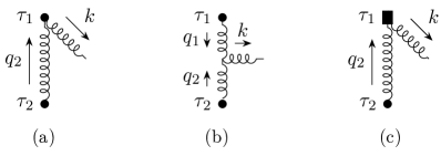
Figure 1: The Feynman diagrams needed for the computation of the stress-energy tensor: (a) and (b) are the point-particle contributions, and (c) is the tidal one. The symmetric terms are obtained by exchange of $1\leftrightarrow 2$.

Stress-energy tensor with tidal effects – The stress-energy tensor needed to compute the emitted four-momentum is given by the sum of the point-particle and tidal contributions, i.e.,

$$\tilde{T}^{\mu\nu}=\tilde{T}_{\rm pp}^{\mu\nu}+\tilde{T}_{\rm tid}^{\mu\nu}\,,$$ (14)

where the tilde denotes the Fourier transform, $\tilde{T}^{\mu\nu}(k)=\int d^{4}x\,T^{\mu\nu}(x)e^{ik\cdot x}$. The stress-energy tensor in the point-particle case was computed in Mougiakakos:2021ckm ; Riva:2021vnj (see also Goldberger:2016iau ). Discarding the static contribution, which does not enter the calculation, the leading-order diagrams are represented in Fig. 1. Using the notation $\int_{q}\equiv\int\frac{d^{4}q}{(2\pi)^{4}}$ and $\delta\!\!\!{}^{-}\!{}^{(n)}(x)\equiv(2\pi)^{n}\delta^{(n)}(x)$, it can be written as

$$\begin{split}&\tilde{T}^{\mu\nu}_{\rm pp}(k)=\frac{m_{1}m_{2}}{4m_{\text{Pl}}^{2}}\int_{q_{1},q_{2}}\!\!\!\delta\!\!\!{}^{-}\!(q_{1}\cdot u_{1})\delta\!\!\!{}^{-}\!(q_{2}\cdot u_{2})\delta\!\!\!{}^{-}\!{}^{(4)}(k-q_{1}-q_{2})\\ &\ \times\frac{e^{iq_{1}\cdot b_{1}+iq_{2}\cdot b_{2}}}{q_{1}^{2}q_{2}^{2}}\left[{t}^{\mu\nu}_{\leavevmode\hbox to3.5pt{\vbox to5.5pt{\text{[drawing]}}}}(q_{1},q_{2})+{t}^{\mu\nu}_{\leavevmode\hbox to3.5pt{\vbox to5.5pt{\text{[drawing]}}}}(q_{1},q_{2})+{t}^{\mu\nu}_{\vdash}(q_{1},q_{2})\right]\,,\end{split}$$ (15)

where ${t}^{\mu\nu}_{\leavevmode\hbox to3.5pt{\vbox to5.5pt{\text{[drawing]}}}}$ is the contribution from diagram (a), ${t}^{\mu\nu}_{\leavevmode\hbox to3.5pt{\vbox to5.5pt{\text{[drawing]}}}}$ from the same diagram but with the two particles exchanged and ${t}^{\mu\nu}_{\vdash}$ from (b). We defer the reader to Ref. Mougiakakos:2021ckm ; Riva:2021vnj for their explicit expressions.

The contribution of the tidal operators to the stress-energy tensor has no static piece. The leading PM term can be obtained from the diagram (c) in Fig. 1 and it is symmetric under exchange of the two particles. We obtain

$$\tilde{T}_{\rm tid}^{\mu\nu}= \ \frac{m_{1}m_{2}}{4m_{\text{Pl}}^{2}}\int_{q_{1},q_{2}}\!\!\!\delta\!\!\!{}^{-}\!(q_{1}\cdot u_{1})\delta\!\!\!{}^{-}\!(q_{2}\cdot u_{2})\delta\!\!\!{}^{-}\!{}^{(4)}(k-q_{1}-q_{2})$$

$$\times\frac{e^{iq_{1}\cdot b_{1}+iq_{2}\cdot b_{2}}}{q_{1}^{2}q_{2}^{2}}\sum_{a=1,2}\sum_{X=E,B}t_{X_{a}^{2}}^{\mu\nu}(q_{1},q_{2})\,,$$ (16)

with $t_{X_{1}^{2}}^{\mu\nu}\equiv-2\frac{c_{X_{1}^{2}}}{m_{1}}q_{1}^{2}\eta^{\mu\alpha}\eta^{\nu\beta}\Pi^{{X}_{1}}_{\alpha\beta,\kappa\lambda}\left(u_{2}^{\kappa}u_{2}^{\lambda}-\eta^{\kappa\lambda}/2\right)$, and an analogous formula for $(1\leftrightarrow 2)$. The explicit expressions of $t_{X_{1}^{2}}^{\mu\nu}$ and $t_{X_{2}^{2}}^{\mu\nu}$ after use of eq. (13), as well as the calculation of the waveform in direct space, are given in the Supplemental Material (SM).

Note that, because of scaling arguments, the tidal contribution vanishes in the soft limit $\omega\rightarrow 0$. As a consequence, at this order in $G$ tidal fields leave no trace on the gravitational wave memory. (See the SM for details.) Since the emitted angular momentum, $J^{\rm rad}$, at $\mathcal{O}(G^{2})$ is proportional to the gravitational wave memory Damour:2020tta , we conclude that there are no tidal effects on the emission of angular momentum at this order. On the other hand, at leading-PM-order the radiation reaction on the scattering angle is related to the radiated angular momentum by $\chi^{\rm rad}=\frac{1}{2}\chi^{\rm cons}_{\rm LO}J^{\rm rad}$ Bini:2012ji ; Damour:2020tta ; Bini:2021gat , where the leading-order conservative contribution to the scattering angle, $\chi^{\rm cons}_{\rm LO}$, is of ${\cal O}(G)$. As a consequence, $\chi^{\rm rad}$ is unaffected by tidal effects at ${\cal O}(G^{3})$.

Radiated four-momentum – The derivation of the emitted linear momentum closely follows the procedure presented in Ref. Riva:2021vnj . In particular, the emitted four-momentum is given as an integral over phase space of the outgoing graviton momentum $k^{\mu}$ weighted by the probability of one graviton emission, which here is given by the square of the total stress-energy tensor from eq. (14). Although we use a quantum mechanical language, this quantity is well defined classically Goldberger:2007hy ; Riva:2021vnj . Defining $\delta\!\!\!{}^{-}\!_{\pm}(k^{2})\equiv\theta(\pm k^{0})\delta\!\!\!{}^{-}\!(k^{2})$ we obtain, for the leading-order contribution from the tidal effects to the radiated momentum,

$$P^{\mu}_{\rm tid}=\frac{1}{2m_{\text{Pl}}^{2}}\int_{k}\delta\!\!\!{}^{-}\!_{+}(k^{2})k^{\mu}\text{Re}\left[\tilde{T}_{\rm pp}^{\alpha\beta}{\mathbb{P}_{\alpha\beta\rho\sigma}}\tilde{T}^{*}_{\rm tid}{}^{\rho\sigma}\right]\;.$$ (17)

From the relation with tidal Love numbers below eq. (4), for $R_{a}\sim Gm_{a}$, the contribution quadratic in $\tilde{T}_{\rm tid}$ is further suppressed by ${\cal O}(G^{4})$ and is thus neglected.

Following Riva:2021vnj , we can interpreted the phase-space delta function as a cut propagator, so that the integrand reproduces a vacuum-to-vacuum diagram with a cut, pictorially represented as

$$\begin{split}&\frac{\delta\!\!\!{}^{-}\!_{+}(k^{2})}{2m_{\text{Pl}}^{2}}\text{Re}\left[\tilde{T}_{\rm pp}^{\alpha\beta}{\mathbb{P}_{\alpha\beta\rho\sigma}}\tilde{T}^{*}_{\rm tid}{}^{\rho\sigma}\right]=\\ {\raisebox{24.0pt}{\scalebox{0.7}{ \leavevmode\hbox to0pt{\vbox to0pt{\text{[drawing]}}} }}}\!\!\!&+{\raisebox{24.0pt}{\scalebox{0.7}{ \leavevmode\hbox to0pt{\vbox to0pt{\text{[drawing]}}} }}}\!\!\!+{\raisebox{24.0pt}{\scalebox{0.7}{ \leavevmode\hbox to0pt{\vbox to0pt{\text{[drawing]}}}}}}\!+(1\leftrightarrow 2)\;,\end{split} c_{X_{1}^{2}} c_{X_{1}^{2}} c_{X_{1}^{2}}$$ (18)

where, using eqs. (LABEL:Tmnpp) and (16) for the stress-energy tensor, the three topologies come from considering the contributions from ${\rm Re}\big{[}{t}^{\alpha\beta}_{\leavevmode\hbox to3.5pt{\vbox to5.5pt{\text{[drawing]}}}}{\mathbb{P}_{\alpha\beta}}^{\rho\sigma}t^{{X}_{1}\,*}_{\rho\sigma}\big{]}$, ${\rm Re}\big{[}{t}^{\alpha\beta}_{\leavevmode\hbox to3.5pt{\vbox to5.5pt{\text{[drawing]}}}}{\mathbb{P}_{\alpha\beta}}^{\rho\sigma}t^{{X}_{1}\,*}_{\rho\sigma}\big{]}$ and ${\rm Re}\big{[}{t}^{\alpha\beta}_{\vdash}{\mathbb{P}_{\alpha\beta}}^{\rho\sigma}t^{{X}_{1}\,*}_{\rho\sigma}\big{]}$, respectively. Notice that the $H$ diagram is absent, because there are no tidal interactions linear in $h_{\mu\nu}$.

We can now recast the problem of computing the emitted momentum as evaluating a cut 2-loop integral followed by a 2d Fourier transform. In particular, the emitted four-momentum can be decomposed without loss of generality along $\check{u}_{1}^{\mu}\equiv(u_{1}^{\mu}-\gamma u_{2}^{\mu})/(1-\gamma^{2})$, $\check{u}_{2}^{\mu}\equiv(u_{2}^{\mu}-\gamma u_{1}^{\mu})/(1-\gamma^{2})$ (satisfying $u_{a}\cdot\check{u}_{b}=\delta_{ab}$), with $\gamma\equiv u_{1}\cdot u_{2}$, and $b^{\mu}$. By the symmetries of the integrand, one can show that the component along $b^{\mu}$ vanishes, so that the momentum can be written as

$$P^{\mu}_{\text{tid}}=\frac{15\pi G^{3}m_{1}^{2}m^{2}_{2}}{64|{\bf b}|^{7}}\sum_{X}\bigg{[}\frac{c_{X_{1}^{2}}}{m_{1}}\Big{(}{\cal E}^{X}\check{u}_{1}^{\mu}+{\cal F}^{X}\check{u}_{2}^{\mu}\Big{)}+(1\leftrightarrow 2)\bigg{]}\,.$$ (19)

The functions ${\cal E}^{X}$ and ${\cal F}^{X}$ inside the brackets depend only on $\gamma$ and can be expressed as 2d Fourier transforms of cut 2-loop integrals, ${\cal I}_{{\cal E}}^{{X}}(\gamma)$ and ${\cal I}_{{\cal F}}^{{X}}(\gamma)$. For instance,

$$\begin{split}{\cal E}^{X}(\gamma)\!=\!|{\bf b}|^{7}\!\!\!\int_{q}&\delta\!\!\!{}^{-}\!(q\cdot u_{1})\delta\!\!\!{}^{-}\!(q\cdot u_{2})e^{iq\cdot b}(-q^{2})^{5/2}{\cal I}_{{\cal E}}^{{X}}(\gamma)\,,\end{split}$$ (20)

and analogously for ${\cal F}^{X}(\gamma)$. The explicit expressions of the 2-loop integrals are given in the SM.

Making use of reverse unitarity Anastasiou:2002yz ; Anastasiou:2002qz ; Anastasiou:2003yy ; Anastasiou:2015yha , we can use IBP identities to express the 2-loop integrals ${\cal I}_{{\cal E},{\cal F}}^{{X}}$ as linear combinations of simpler master integrals. We perform this reduction using the Mathematica package LiteRed Lee:2012cn ; Lee:2013mka , finding that the three integrals defined in eqs. (4.13)–(4.15) of Ref. Riva:2021vnj form a complete base. (In the minimally coupled case we need a fourth integral, defined in eq. (4.16) of this reference. This comes from the $H$ diagram, which here is absent.) These integrals can be solve using differential equation methods Kotikov:1990kg ; Bern:1992em ; Gehrmann:1999as ; Henn:2013pwa ; Caron-Huot:2014lda ; Henn:2014qga ; Parra-Martinez:2020dzs . Eventually, we find that

$${\cal E}^{X}=f_{1}^{{X}}+f_{2}^{{X}}\log\left(\frac{\gamma+1}{2}\right)+f_{3}^{{X}}\frac{\text{arccosh}(\gamma)}{\sqrt{\gamma^{2}-1}}\;,$$ (21)

with $f_{1}^{{X}}$, $f_{2}^{{X}}$, $f_{3}^{{X}}$ and ${\cal F}^{X}$ given in Table 1.

$$f^{E}_{1} =\frac{1}{2(\gamma+1)^{3}\sqrt{\gamma^{2}-1}}\Big{[}937\gamma^{9}+1551\gamma^{8}-2463\gamma^{7}-5645\gamma^{6}$$ $$+20415\gamma^{5}+65965\gamma^{4}-349541\gamma^{3}+535057\gamma^{2}-360356\gamma+92160\Big{]}\,$$ $$f^{B}_{1} =\frac{\gamma-1}{4(\gamma+1)^{3}\sqrt{\gamma^{2}-1}}\Big{[}1559\gamma^{8}+3716\gamma^{7}-1630\gamma^{6}-11660\gamma^{5}$$ $$-28288\gamma^{4}+155292\gamma^{3}-543442\gamma^{2}+535212\gamma-180775\Big{]}\,$$ $$f^{E}_{2} ={30\sqrt{\gamma^{2}-1}\left(21\gamma^{4}-14\gamma^{2}+9\right)}\,,$$ $$f^{B}_{2} =210(\gamma^{2}-1)^{3/2}\left(1+3\gamma^{2}\right)\;,\qquad f^{X}_{3}=-{f^{X}_{2}}\frac{\gamma(2\gamma^{2}-3)}{4(\gamma^{2}-1)}\,$$ $${\cal F}^{E} =\frac{3(\gamma-1)^{2}}{(\gamma+1)^{3}\sqrt{\gamma^{2}-1}}\Big{[}42\gamma^{8}+210\gamma^{7}+315\gamma^{6}-105\gamma^{5}-944\gamma^{4}$$ $$-1528\gamma^{3}+22011\gamma^{2}-33201\gamma+16272\Big{]}\,$$ $${\cal F}^{B} =-\frac{3(\gamma-1)^{3}(105\gamma^{5}+630\gamma^{4}\!+\!1840\gamma^{3}\!+3690\gamma^{2}\!-\!17769\gamma+15984)}{(\gamma+1)^{3}\sqrt{\gamma^{2}-1}}\,$$

Table 1: Functions specifying the radiated four-momentum in eq. (19).

From eq. (19), one can compute the radiated energy in the center-of-mass frame from tidal effects, $\Delta E_{\rm tid}\equiv P_{\rm tid}\cdot u_{\rm c.m.}$. Defining the total mass $m\equiv m_{1}+m_{2}$, the symmetric mass ratio $\nu\equiv m_{1}m_{2}/m^{2}$ and $h(\nu,\gamma)\equiv E/m=\sqrt{1+2\nu(\gamma-1)}$, where $E$ is the incoming energy of the two-body system, this reads

$$\Delta E_{\rm tid}=\frac{15\pi G^{7}m^{8}\nu^{2}}{64|{\bf b}|^{7}h}{\cal G}({\cal E}^{X},{\cal F}^{X})\,,$$ (22)

where

$${\cal G}({\cal E}^{X},{\cal F}^{X})\equiv\sum_{X}\left[\kappa_{X^{2}}{\cal E}^{X}\!+\lambda_{X^{2}}({\cal F}^{X}-{\cal E}^{X})\right]\,,$$ (23)

and we have introduced the dimensionless parameters Kalin:2020lmz

$$\lambda_{X^{2}} \equiv\frac{1}{G^{4}m^{5}}\left(\frac{c_{X_{1}^{2}}m_{2}}{m_{1}}+\frac{c_{X_{2}^{2}}m_{1}}{m_{2}}\right)\;,$$ (24)

$$\kappa_{X^{2}} \equiv\frac{1}{G^{4}m^{4}}\left(\frac{c_{X_{1}^{2}}}{m_{1}}+\frac{c_{X_{2}^{2}}}{m_{2}}\right)\;.$$ (25)

Expanding for small velocities $v\equiv\sqrt{\gamma^{2}-1}/\gamma$, we find

$$\begin{split}{\cal E}^{E}&=288v^{3}+\frac{2143}{7}v^{5}+\frac{14542}{21}v^{7}+{\cal O}(v^{9})\;,\\ {\cal E}^{B}&=-98v^{5}+\frac{585}{4}v^{7}+{\cal O}(v^{9})\;,\\ {\cal F}^{E}&=288v^{3}+336v^{5}+\frac{3027}{4}v^{7}+{\cal O}(v^{9})\;,\\ {\cal F}^{B}&=-210v^{5}-\frac{669}{4}v^{7}+{\cal O}(v^{9})\;,\end{split}$$ (26)

which shows that the current (magnetic) quadrupole is 1PN order higher than the mass (electric) one, as expected.

Finally, the emitted energy from a two-body encounter can be used to derive the energy loss for closed orbits by the use of the B2B relation Kalin:2019rwq ; Kalin:2019inp ; Bini:2020hmy ; Cho:2021arx , $\Delta E^{\rm(closed)}(\gamma,J)=\Delta E^{\rm(open)}(\gamma,J)-\Delta E^{\rm(open)}(\gamma,-J)$, where the emitted energy on the right-hand side must be expressed in terms of the angular momentum $J=|{\bf b}|m\nu\sqrt{\gamma^{2}-1}/h(\nu,\gamma)$ (with $h=E/m$) and analytically continued to bound orbits with $h<1$, corresponding to $\gamma=1+\frac{h^{2}-1}{2\nu}<1$. This yields

$$\Delta E^{\rm(closed)}_{\rm tid}=\frac{15\pi G^{7}m^{15}\nu^{9}(1-\gamma^{2})^{7/2}}{64J^{7}h^{8}}{\cal G}(\tilde{\cal E}^{X},\tilde{\cal F}^{X})\\$$ (27)

where

$$\tilde{\cal E}^{X} =\tilde{f}_{1}^{{X}}+\tilde{f}_{2}^{{X}}\log\left(\frac{\gamma+1}{2}\right)+\tilde{f}_{3}^{{X}}\frac{\text{arccos}(\gamma)}{\sqrt{1-\gamma^{2}}}\,,$$ (28)

with $\tilde{f}_{1}^{X}=-2f_{1}^{X}$, $\tilde{f}_{2}^{E}=-2f_{2}^{E}$, $\tilde{f}_{2}^{B}=2f_{2}^{B}$, $\tilde{f}_{3}^{E}=2f_{3}^{E}$, $\tilde{f}_{3}^{B}=-2f_{3}^{B}$ and $\tilde{\cal F}^{X}=-2{\cal F}^{X}$, all subject to the replacement $(\gamma^{2}-1)^{n/2}\to(1-\gamma^{2})^{n/2}$. In the following we show that this expression is consistent with known results in the PN approximation.

Radiated Flux – The instantaneous flux is defined as $F\equiv dE/dt$. Focussing on the tidal correction, $F_{\rm tid}$, and integrating this relation for half of the scattering trajectory, we obtain

$$\Delta E_{\rm tid}(\gamma)=2\int_{|{\bf b}|}^{\infty}\!\frac{dr}{\dot{r}}F_{\rm tid}(r,\gamma)\,.$$ (29)

We have assumed that the expression of the flux is in isotropic gauge; thus, we have dropped the dependence on $J$ in $F_{\rm tid}$. From eq. (22), the leading-order tidal contribution to the flux scales as $G^{7}$ so that its dependence on $r$ is fully determined: $F_{{\rm tid}}(r,\gamma)\propto r^{-8}$. By integrating the right-hand side of eq. (29) with this ansatz, and using $\dot{r}$ for straight orbits at this PM order, we find

$$F_{{\rm tid}}(r,\gamma)=\frac{G^{7}m^{8}}{r^{8}}\frac{3\nu^{3}\sqrt{\gamma^{2}-1}}{4h^{3}\xi}{\cal G}({\cal E}^{X},{\cal F}^{X})\,,$$ (30)

where $\xi\equiv E_{1}E_{2}/E^{2}$, and $E_{a}$ is the initial asymptotic energies of body $a=1,2$. This result extends the one for point-particles computed in Cho:2021arx . As discussed there, due to the absence of a term higher in $G$, the leading PM computation is insufficient to reconstruct the leading PN flux but it provides the full velocity–or reduced-energy–series to order $G^{3}$.

Consistency check – We can compare our result for small velocities to the emitted flux and energy in one period derived in the PN expansion in the large eccentricity limit, i.e. to leading order in large $J$.

The tidal effects on the gravitational wave energy flux for spinless bodies has been computed up to the next-to-next-to-leading PN order in Henry:2020ski (see Henry:2019xhg ; Henry:2020pzq for a derivation of the equations of motion and Hamiltonian in this case, respectively; see also Huber:2020xny for a calculation of the PM Hamiltonian and the emitted energy for quasi-circular orbits at leading PN order, with interactions cubic in the curvature and tidal effects). Although in that reference the results were given only for quasi-circular orbits, their authors have kindly provided us with an expression of the flux $F_{\rm tid}^{\rm(PN)}$ and the conserved energy $E$ and angular momentum $J$ for generic orbits, written in terms of $r$, $\dot{r}$ and $\dot{\phi}$, respectively the two-body distance, the radial velocity and the angular velocity in the center-of-mass frame. We have used the expressions for $E$ and $J$ to replace $\dot{r}=\dot{r}(r,E,J)$ and $\dot{\phi}=\dot{\phi}(r,E,J)$ in the flux and we have computed the emitted energy for generic closed orbits by integrating it in the variable $r$ over one period.

The resulting energy reduces to that given in Henry:2020ski for circular orbits. Moreover, it is consistent with the expansion eq. (26) (taking into account the factor of -2 according to eq. (27)). Since all the powers of $\gamma$ in Table 1 intervene in this expansion, this is a rather nontrivial check of our calculation. Moreover, the PN flux $F_{\rm tid}^{\rm(PN)}$ coincides with the low-velocity expansion of eq. (30), up to total derivatives in the balance equations–the so-called Schott terms. Although the two fluxes are written in different gauges (in harmonic and isotropic gauge, respectively in Ref. Henry:2020ski and in eq. (30)) the gauge difference is 2PM orders higher and can be neglected. For the reader’s convenience, we report the explicit expression of the PM flux in the ancillary file submitted with the arXiv version of this article.

High-energy limit – Going back to the energy loss for hyperbolic-like orbits, eq. (22), for large $\gamma$ we find ${\cal E}_{\rm HE}^{X}=(a_{X}+b_{X}\log\gamma)\gamma^{5}+{\cal O}(\gamma^{3})$ and ${\cal F}_{\rm HE}^{X}=c_{X}\gamma^{6}+d_{X}\gamma^{4}+{\cal O}(\gamma^{2})$, with $a_{E}=937/2-945\log 2$, $a_{B}=1559/4-945\log 2$, $b_{E}=b_{B}=315$, $c_{E}=126$, $c_{B}=0$, $d_{E}=-504$ and $d_{B}=-315$. While ${\cal E}_{\rm HE}^{E}$ and ${\cal E}_{\rm HE}^{B}$ scale in the same way with $\gamma$, ${\cal F}_{\rm HE}^{E}$ and ${\cal F}_{\rm HE}^{B}$ behave differently. Our perturbative expansion is valid for $\gamma(Gm/|{\bf b}|)\ll 1$ DEath:1976bbo ; Damour:2019lcq ; DiVecchia:2022nna (see also Kovacs:1978eu ). In this regime $\Delta E_{\rm tid}\ll\Delta E\sim(Gm/|{\bf b}|)^{3}(m/h)\gamma^{3}\ll E$.

Conclusion – We have computed the four-momentum and the flux emitted in gravitational waves by the scattering of tidally interacting bodies at leading order in the post-Minkowskian approximation. Our computation uses the worldline effective field theory approach and the results obtained are, up to our knowledge, new. We focused on electric and magnetic-type quadrupolar effects but our computations can be straightforwardly extended to higher multipoles or to higher-orders in the curvature fields.

We have derived the emitted energy for bound orbits using the B2B dictionary and verified that it is consistent with PN results for eccentric orbits. Considering the ultra-relativistic limit of the energy loss, we observe that the contributions of the electric and magnetic component scale differently unlike the case of the conservative scattering angle. It would be interesting to use the derived PM flux to study the corresponding modifications of the waveform.

Acknowledgements – We thank Luc Blanchet, Guillaume Faye and Quentin Henry for helpful discussions and for kindly providing us with expressions of the flux, conserved energy and angular momentum for generic orbits. We also thank Thibault Damour, Carlo Heissenberg, Enrico Herrmann, Gregor Kälin, Alessandro Nagar, Rafael Porto, Rodolfo Russo and Leong Khim Wong for interesting discussions and comments on the draft. This work was partially supported by the CNES.

Tidal stress-energy tensor

Here we give the explicit expression of the tidal stress-energy tensor defined in eq. (16). Introducing $\beta\equiv 2\gamma^{2}-1$ and $\omega_{a}=k\cdot u_{a}$, we have

$$\frac{m_{1}}{q_{1}^{2}}\frac{t_{E_{1}^{2}}^{\mu\nu}}{c_{E_{1}^{2}}}=\omega_{1}^{4}\eta^{\mu\nu}-\beta\omega_{1}^{2}q_{2}^{\mu}q_{2}^{\nu}-2\omega_{1}^{3}q_{1}^{(\mu}u_{1}^{\nu)}$$

$$-\omega_{1}\left(\beta q_{1}^{2}+4\gamma\omega_{1}\omega_{2}+2\omega_{1}^{2}\right)q_{2}^{(\mu}u_{1}^{\nu)}+4\gamma\omega_{1}^{3}q_{2}^{(\mu}u_{2}^{\nu)}$$

$$-\left(\beta{q_{1}^{4}}/{4}+2\gamma\omega_{1}\omega_{2}q_{1}^{2}+2\omega_{1}^{2}\omega_{2}^{2}\right)u_{1}^{\mu}u_{1}^{\nu}$$

$$-2\omega_{1}^{4}u_{2}^{\mu}u_{2}^{\nu}+2\omega_{1}^{2}\left(\gamma{q_{1}^{2}}+2\omega_{1}\omega_{2}\right)u_{1}^{(\mu}u_{2}^{\nu)}$$ (31)

$$\frac{m_{1}}{q_{1}^{2}}\frac{t_{B_{1}^{2}}^{\mu\nu}}{c_{B_{1}^{2}}}=\omega_{1}^{2}({q_{1}^{2}}/{2}+\omega_{1}^{2})\eta^{\mu\nu}-\omega_{1}\left(\beta\omega_{1}-2\gamma\omega_{2}\right)q_{2}^{\mu}q_{2}^{\nu}$$

$$+\omega^{2}_{1}q_{1}^{(\mu}q_{2}^{\nu)}-\frac{1}{2}(\gamma{q_{1}^{2}}+2\omega_{1}\omega_{2})^{2}u_{1}^{\mu}u_{1}^{\nu}-\omega_{1}^{2}({q_{1}^{2}}+2\omega_{1}^{2})u_{2}^{\mu}u_{2}^{\nu}$$

$$+({q_{1}^{2}}/{2}+2\omega_{1}^{2})(\gamma{q_{1}^{2}}+2\omega_{1}\omega_{2})u_{1}^{(\mu}u_{2}^{\nu)}-\left(2\omega_{1}(\omega_{1}^{2}-\omega_{2}^{2}+\right.$$

$$\left.+2\gamma\omega_{1}\omega_{2})+{q_{1}^{2}}((1+4\gamma^{2})\omega_{1}-2\gamma\omega_{2})/2\right)q_{2}^{(\mu}u_{1}^{\nu)}+\omega_{1}(\gamma{q_{1}^{2}}$$

$$+4\gamma\omega_{1}^{2}-2\omega_{1}\omega_{2})q_{2}^{(\mu}u_{2}^{\nu)}-\omega_{1}({q_{1}^{2}}/{2}+2\omega_{1}^{2})q_{1}^{(\mu}u_{1}^{\nu)}\,,$$ (32)

and analogous expressions for $t_{X_{2}^{2}}^{\mu\nu}$ with $(1\leftrightarrow 2)$.

Waveform

The asymptotic waveform in direct space, i.e. $h_{\lambda}\equiv\epsilon^{\mu\nu}_{\lambda}h_{\mu\nu}/m_{\text{Pl}}$, with $\lambda=\pm$, evaluated at distances $r$ much larger than the interaction region, reads

$$h_{\lambda}(x) =\frac{4G}{r}\int\frac{dk^{0}}{2\pi}e^{-ik^{0}u}\epsilon^{\lambda*}_{\alpha\beta}\tilde{T}^{\alpha\beta}|_{k^{\mu}=k^{0}n^{\mu}}\;,$$ (33)

where $u\equiv t-r$ is the retarded time. The stress-energy tensor on the right-hand side is evaluated on-shell, i.e. $k^{\mu}=k^{0}n^{\mu}$, with $n^{\mu}\equiv(1,{\bf n})$ and ${\bf n}^{2}=1$.

In the point-particle case, the waveform was computed using our approach in Mougiakakos:2021ckm (see also Jakobsen:2021smu ), in agreement with earlier calculations Thorne:1975aa . Here we focus on the tidal contribution, obtained by replacing (16) in the above expression. Integrating first in $k^{0}$, we obtain

$$h_{\lambda}^{\rm tid}= \!\!\!\sum_{X={E,B}}\!\!\!c_{X^{2}_{1}}\frac{Gm_{2}}{r\,m_{\text{Pl}}^{2}}\frac{\epsilon^{*\lambda}_{\mu\nu}({\bf n})}{n\cdot u_{1}}\int_{q}\frac{\delta\!\!\!{}^{-}\!(q\cdot u_{2})e^{iq\cdot\tilde{b}}}{q^{2}(k-q)^{2}}$$

$$\times{t_{X_{1}^{2}}^{\mu\nu}}(q-k,q)\big{|}_{k^{0}=\frac{q\cdot u_{1}}{n\cdot u_{1}}}+(1\leftrightarrow 2),$$ (34)

where $\tilde{b}\equiv b+\frac{u_{1}}{n\cdot u_{1}}(u+{\bf n}\cdot{\bf b}_{1})$. We can then choose a frame and remove the remaining delta function by integrating in $q^{0}$. Regardless of the chosen frame, the remaining integral can be put in the form of the master integral

$$I=\int_{\bf{q}}\frac{e^{i\bf{q}\cdot\bf{b}}}{{\bf q}\cdot{\bf M}\cdot{\bf q}}=\frac{1}{4\pi}\frac{\left[{\bf b}\cdot{\bf M}^{-1}\cdot{\bf b}\right]^{-1/2}}{\left[\text{det}(\bf{M})\right]^{1/2}}\;,$$ (35)

where ${\bf M}$ is a $3\times 3$ matrix, or of its tensorial generalization, $I^{i_{1},...,i_{n}}=\int_{\bf{q}}\frac{{\bf q}^{i_{1}}\cdots{\bf q}^{i_{n}}e^{i\bf{q}\cdot\bf{b}}}{{\bf q}\cdot{\bf M}\cdot{\bf q}}$, which can be solved by taking derivatives of the master integral, $I^{i_{1},...,i_{n}}=\frac{\partial}{i\partial b_{i_{1}}}...\frac{\partial}{i\partial b_{i_{n}}}I$.

Performing the calculation in the rest frame of particle 2, i.e. for $u_{1}^{\mu}=\gamma(1,v\hat{{\bf v}})$ and $u_{2}^{\mu}=\delta^{\mu}_{0}$, and choosing $b_{1}^{\mu}=(0,{\bf b})$ and $b_{2}^{\mu}=0$ for simplicity, we obtain

$$h_{\lambda}^{\rm tid}=120\frac{G^{2}m_{1}m_{2}}{r}\frac{\gamma^{2}v^{2}}{|{\bf b}|^{5}}\sum_{a=1,2}\sum_{X={E,B}}\frac{c_{X_{a}^{2}}}{m_{a}}\frac{\epsilon^{*\lambda}_{ij}{\bf e}_{I}^{i}{\bf e}_{J}^{j}A^{IJ}_{X_{a}^{2}}}{(n\cdot u_{a})^{3}{c}_{a}^{9/2}}\,,$$ (36)

where we have defined ${\bf e}_{I}\equiv(\hat{\bf v},\hat{\bf b})$ (with $I=v,b$), and the functions ${c_{1}}=1+\frac{\gamma^{2}v^{2}}{(n\cdot u_{1})^{2}}\big{(}\frac{u}{|{\bf b}|}+{\bf n}\cdot\hat{{\bf b}}\big{)}^{2}$ and ${c_{2}}=1+\gamma^{2}v^{2}\frac{u^{2}}{|{\bf b}|^{2}}$. Defining $f_{a}=6c_{a}-7$, $g_{a}=\sqrt{c_{a}-1}(4c_{a}-7)$, the explicit expressions for $A^{IJ}_{X_{a}^{2}}$ are

$$A^{bb}_{{E}_{a}^{2}}={(n\cdot u_{a})^{2}}\beta f_{a}\;,$$

$$A^{vb}_{{E}_{a}^{2}}=\gamma(n\cdot u_{a})\big{[}f_{a}\beta v\delta_{a1}\hat{{\bf b}}\cdot{\bf n}+g_{a}\big{]}\;,$$

$$A^{vv}_{{E}_{a}^{2}}=\frac{(2f_{a}^{2}-17f_{a}-7)}{30}+f_{a}(\gamma^{2}-1)$$

$$+v\gamma^{2}\delta_{a1}\hat{{\bf b}}\cdot{\bf n}\big{[}f_{a}\beta v\delta_{a1}\hat{{\bf b}}\cdot{\bf n}+2g_{a}\big{]}\;,$$

$$A^{bb}_{{B}_{a}^{2}}=2\gamma{(n\cdot u_{a})}\big{[}\gamma\ n\cdot u_{a}-\frac{(n\cdot u_{1})(n\cdot u_{2})}{n\cdot u_{a}}\big{]}f_{a}\;,$$

$$A^{vb}_{{B}_{a}^{2}}=f_{a}\gamma^{2}(2\gamma\delta_{a1}n\cdot u_{a}-1)v\hat{{\bf b}}\cdot{\bf n}$$

$$+g_{a}\big{[}\gamma\ n\cdot u_{a}-\frac{(n\cdot u_{1})(n\cdot u_{2})}{n\cdot u_{a}}\big{]}\;,$$

$$A^{vv}_{{B}_{a}^{2}}=2\gamma^{2}v\hat{{\bf b}}\cdot{\bf n}\big{[}f_{a}\gamma^{2}v\delta_{a1}\hat{{\bf b}}\cdot{\bf n}+\frac{\gamma\delta_{a1}-\delta_{a2}}{\gamma}g_{a}\big{]}\;.$$ (37)

One can verify that, upon PN expanding, the contribution of the current (magnetic) quadrupole enters at 1PN higher than the mass (electric) one, as expected.

Note, also, that the gravitational wave memory, i.e., the difference in the waveform between asymptotic past and future, defined as

$$\Delta h_{\lambda}({\bf x})\equiv\int_{-\infty}^{+\infty}du\ \dot{h}_{\lambda}(u,{\bf x})\;,$$ (38)

is not affected by tidal deformations at this order in $G$. Indeed, from eq. (33) the contribution of tidal effects to the memory reads

$$\Delta h^{\rm tid}_{\lambda}=-i\frac{4G}{r}\int\frac{dk^{0}}{2\pi}\delta\!\!\!{}^{-}\!(k^{0})k^{0}\,\epsilon^{\lambda*}_{\alpha\beta}\tilde{T}^{\alpha\beta}_{\rm tid}|_{k^{\mu}=k^{0}n^{\mu}}\;.$$ (39)

From eqs. (31) and (32) above, $\tilde{T}_{\rm tid}^{\mu\nu}\sim\mathcal{O}((k^{0})^{4})$ and thus the right-hand side of this equation vanishes. This conclusion can be extended to higher-order tidal fields, which contribute to $\tilde{T}_{\rm tid}$ higher in $k^{0}$.

2-loop integrals

Introducing the following basis of propagators

$$\rho_{1} =2\ell_{1}\cdot u_{1}\,, \rho_{2} =-2\ell_{1}\cdot u_{2}\,, \rho_{3} =-2\ell_{2}\cdot u_{1}\,$$

$$\rho_{4} =2\ell_{2}\cdot u_{2}\,, \rho_{5} =\ell_{1}^{2}\,, \rho_{6} =\ell_{2}^{2}\,,$$ (40)

$$\rho_{7} =(\ell_{1}+\ell_{2}-q)^{2}\,, \rho_{8} =(\ell_{1}-q)^{2}\,, \rho_{9} =(\ell_{2}-q)^{2}\,,$$

we can explicitly write the 2-loop integrals in eq. (20) as

$${\cal I}^{X}_{\cal E} =\frac{2^{17}\pi^{2}}{15(-q^{2})}\frac{m_{1}}{c_{X_{1}^{2}}}\int_{\ell_{1},\ell_{2}}\!\!\!\!\!\delta\!\!\!{}^{-}\!_{-}(\rho_{7})\delta\!\!\!{}^{-}\!(\rho_{1})\delta\!\!\!{}^{-}\!(\rho_{4})\frac{\rho_{3}\,{\cal N}_{X_{1}}}{\rho_{5}\rho_{6}\rho_{8}\rho_{9}}\,,$$ (41)

$${\cal I}^{X}_{\cal F} =\frac{2^{17}\pi^{2}}{15(-q^{2})}\frac{m_{2}}{c_{X_{2}^{2}}}\int_{\ell_{1},\ell_{2}}\!\!\!\!\!\delta\!\!\!{}^{-}\!_{-}(\rho_{7})\delta\!\!\!{}^{-}\!(\rho_{1})\delta\!\!\!{}^{-}\!(\rho_{4})\frac{\rho_{3}\,{\cal N}_{X_{2}}}{\rho_{5}\rho_{6}\rho_{8}\rho_{9}}\,,$$ (42)

where ${\cal N}_{X_{a}}\equiv{\rm Re}\left[\left({t}^{\alpha\beta}_{\leavevmode\hbox to3.5pt{\vbox to5.5pt{\text{[drawing]}}}}+{t}^{\alpha\beta}_{\leavevmode\hbox to3.5pt{\vbox to5.5pt{\text{[drawing]}}}}+{t}^{\alpha\beta}_{\vdash}\right){\mathbb{P}_{\alpha\beta}}^{\rho\sigma}t^{{X}_{a}\,*}_{\rho\sigma}\right]$.

References

- (1) Virgo, LIGO Scientific Collaboration, B. P. Abbott et. al., “Observation of Gravitational Waves from a Binary Black Hole Merger,” Phys. Rev. Lett. 116 (2016), no. 6 061102, 1602.03837.
- (2) Virgo, LIGO Scientific Collaboration, B. P. Abbott et. al., “GW170817: Observation of Gravitational Waves from a Binary Neutron Star Inspiral,” Phys. Rev. Lett. 119 (2017), no. 16 161101, 1710.05832.
- (3) E. Berti et. al., “Testing General Relativity with Present and Future Astrophysical Observations,” Class. Quant. Grav. 32 (2015) 243001, 1501.07274.
- (4) E. Barausse et. al., “Prospects for Fundamental Physics with LISA,” Gen. Rel. Grav. 52 (2020), no. 8 81, 2001.09793.
- (5) T. Damour, M. Soffel, and C.-m. Xu, “General relativistic celestial mechanics. 3. Rotational equations of motion,” Phys. Rev. D 47 (1993) 3124–3135.
- (6) T. Damour, M. Soffel, and C.-m. Xu, “General relativistic celestial mechanics. 4: Theory of satellite motion,” Phys. Rev. D 49 (1994) 618–635.
- (7) W. D. Goldberger and I. Z. Rothstein, “Dissipative effects in the worldline approach to black hole dynamics,” Phys. Rev. D 73 (2006) 104030, hep-th/0511133.
- (8) T. Hinderer, “Tidal Love numbers of neutron stars,” Astrophys. J. 677 (2008) 1216–1220, 0711.2420.
- (9) E. E. Flanagan and T. Hinderer, “Constraining neutron star tidal Love numbers with gravitational wave detectors,” Phys. Rev. D 77 (2008) 021502, 0709.1915.
- (10) T. Damour and A. Nagar, “Relativistic tidal properties of neutron stars,” Phys. Rev. D 80 (2009) 084035, 0906.0096.
- (11) T. Binnington and E. Poisson, “Relativistic theory of tidal Love numbers,” Phys. Rev. D 80 (2009) 084018, 0906.1366.
- (12) T. Hinderer, B. D. Lackey, R. N. Lang, and J. S. Read, “Tidal deformability of neutron stars with realistic equations of state and their gravitational wave signatures in binary inspiral,” Phys. Rev. D 81 (2010) 123016, 0911.3535.
- (13) B. Kol and M. Smolkin, “Black hole stereotyping: Induced gravito-static polarization,” JHEP 02 (2012) 010, 1110.3764.
- (14) T. Damour, A. Nagar, and L. Villain, “Measurability of the tidal polarizability of neutron stars in late-inspiral gravitational-wave signals,” Phys. Rev. D 85 (2012) 123007, 1203.4352.
- (15) M. Favata, “Systematic parameter errors in inspiraling neutron star binaries,” Phys. Rev. Lett. 112 (2014) 101101, 1310.8288.
- (16) L. Baiotti and L. Rezzolla, “Binary neutron star mergers: a review of Einstein’s richest laboratory,” Rept. Prog. Phys. 80 (2017), no. 9 096901, 1607.03540.
- (17) L. Barack et. al., “Black holes, gravitational waves and fundamental physics: a roadmap,” Class. Quant. Grav. 36 (2019), no. 14 143001, 1806.05195.
- (18) A. Buonanno and B. S. Sathyaprakash, Sources of Gravitational Waves: Theory and Observations. 10, 2014. 1410.7832.
- (19) V. Cardoso and P. Pani, “Testing the nature of dark compact objects: a status report,” Living Rev. Rel. 22 (2019), no. 1 4, 1904.05363.
- (20) D. Baumann, H. S. Chia, R. A. Porto, and J. Stout, “Gravitational Collider Physics,” Phys. Rev. D 101 (2020), no. 8 083019, 1912.04932.
- (21) T. Mora and C. M. Will, “A PostNewtonian diagnostic of quasiequilibrium binary configurations of compact objects,” Phys. Rev. D 69 (2004) 104021, gr-qc/0312082. [Erratum: Phys.Rev.D 71, 129901 (2005)].
- (22) J. E. Vines and E. E. Flanagan, “Post-1-Newtonian quadrupole tidal interactions in binary systems,” Phys. Rev. D 88 (2013) 024046, 1009.4919.
- (23) J. Vines, E. E. Flanagan, and T. Hinderer, “Post-1-Newtonian tidal effects in the gravitational waveform from binary inspirals,” Phys. Rev. D 83 (2011) 084051, 1101.1673.
- (24) Q. Henry, G. Faye, and L. Blanchet, “Tidal effects in the equations of motion of compact binary systems to next-to-next-to-leading post-Newtonian order,” Phys. Rev. D 101 (2020), no. 6 064047, 1912.01920.
- (25) Q. Henry, G. Faye, and L. Blanchet, “Hamiltonian for tidal interactions in compact binary systems to next-to-next-to-leading post-Newtonian order,” Phys. Rev. D 102 (2020), no. 12 124074, 2009.12332.
- (26) Q. Henry, G. Faye, and L. Blanchet, “Tidal effects in the gravitational-wave phase evolution of compact binary systems to next-to-next-to-leading post-Newtonian order,” Phys. Rev. D 102 (2020), no. 4 044033, 2005.13367.
- (27) T. Damour and A. Nagar, “Effective One Body description of tidal effects in inspiralling compact binaries,” Phys. Rev. D 81 (2010) 084016, 0911.5041.
- (28) D. Bini, T. Damour, and G. Faye, “Effective action approach to higher-order relativistic tidal interactions in binary systems and their effective one body description,” Phys. Rev. D 85 (2012) 124034, 1202.3565.
- (29) J. Steinhoff, T. Hinderer, A. Buonanno, and A. Taracchini, “Dynamical Tides in General Relativity: Effective Action and Effective-One-Body Hamiltonian,” Phys. Rev. D94 (2016) 104028, 1608.01907.
- (30) W. D. Goldberger and I. Z. Rothstein, “An Effective field theory of gravity for extended objects,” Phys. Rev. D 73 (2006) 104029, hep-th/0409156.
- (31) W. D. Goldberger, “Les Houches lectures on effective field theories and gravitational radiation,” in Les Houches Summer School - Session 86: Particle Physics and Cosmology: The Fabric of Spacetime, 1, 2007. hep-ph/0701129.
- (32) S. Foffa and R. Sturani, “Effective field theory methods to model compact binaries,” Class. Quant. Grav. 31 (2014), no. 4 043001, 1309.3474.
- (33) I. Z. Rothstein, “Progress in effective field theory approach to the binary inspiral problem,” Gen. Rel. Grav. 46 (2014) 1726.
- (34) R. A. Porto, “The effective field theorist’s approach to gravitational dynamics,” Phys. Rept. 633 (2016) 1–104, 1601.04914.
- (35) M. Levi, “Effective Field Theories of Post-Newtonian Gravity: A comprehensive review,” Rept. Prog. Phys. 83 (2020), no. 7 075901, 1807.01699.
- (36) D. Bini and T. Damour, “Gravitational self-force corrections to two-body tidal interactions and the effective one-body formalism,” Phys. Rev. D 90 (2014), no. 12 124037, 1409.6933.
- (37) D. Bini and A. Geralico, “Gravitational self-force corrections to tidal invariants for spinning particles on circular orbits in a Schwarzschild spacetime,” Phys. Rev. D 98 (2018), no. 8 084021, 1806.03495.
- (38) D. Bini and A. Geralico, “Gravitational self-force corrections to tidal invariants for particles on eccentric orbits in a Schwarzschild spacetime,” Phys. Rev. D 98 (2018), no. 6 064026, 1806.06635.
- (39) D. Bini and A. Geralico, “Gravitational self-force corrections to tidal invariants for particles on circular orbits in a Kerr spacetime,” Phys. Rev. D 98 (2018), no. 6 064040, 1806.08765.
- (40) T. Dietrich, T. Hinderer, and A. Samajdar, “Interpreting Binary Neutron Star Mergers: Describing the Binary Neutron Star Dynamics, Modelling Gravitational Waveforms, and Analyzing Detections,” Gen. Rel. Grav. 53 (2021), no. 3 27, 2004.02527.
- (41) B. Bertotti, “On gravitational motion,” Nuovo Cim. 4 (1956), no. 4 898–906.
- (42) B. Bertotti and J. Plebanski, “Theory of gravitational perturbations in the fast motion approximation,” Annals Phys. 11 (1960), no. 2 169–200.
- (43) P. Havas and J. N. Goldberg, “Lorentz-Invariant Equations of Motion of Point Masses in the General Theory of Relativity,” Phys. Rev. 128 (1962) 398–414.
- (44) K. Westpfahl and M. Goller, “GRAVITATIONAL SCATTERING OF TWO RELATIVISTIC PARTICLES IN POSTLINEAR APPROXIMATION,” Lett. Nuovo Cim. 26 (1979) 573–576.
- (45) M. Portilla, “SCATTERING OF TWO GRAVITATING PARTICLES: CLASSICAL APPROACH,” J. Phys. A 13 (1980) 3677–3683.
- (46) L. Bel, T. Damour, N. Deruelle, J. Ibanez, and J. Martin, “Poincaré-invariant gravitational field and equations of motion of two pointlike objects: The postlinear approximation of general relativity,” Gen. Rel. Grav. 13 (1981) 963–1004.
- (47) K. Westpfahl, “High-Speed Scattering of Charged and Uncharged Particles in General Relativity,” Fortsch. Phys. 33 (1985), no. 8 417–493.
- (48) T. Damour, “Gravitational scattering, post-Minkowskian approximation and Effective One-Body theory,” Phys. Rev. D 94 (2016), no. 10 104015, 1609.00354.
- (49) T. Damour, “High-energy gravitational scattering and the general relativistic two-body problem,” Phys. Rev. D 97 (2018), no. 4 044038, 1710.10599.
- (50) D. Bini and T. Damour, “Gravitational spin-orbit coupling in binary systems, post-Minkowskian approximation and effective one-body theory,” Phys. Rev. D 96 (2017), no. 10 104038, 1709.00590.
- (51) D. Bini and T. Damour, “Gravitational spin-orbit coupling in binary systems at the second post-Minkowskian approximation,” Phys. Rev. D 98 (2018), no. 4 044036, 1805.10809.
- (52) J. Vines, J. Steinhoff, and A. Buonanno, “Spinning-black-hole scattering and the test-black-hole limit at second post-Minkowskian order,” Phys. Rev. D 99 (2019), no. 6 064054, 1812.00956.
- (53) T. Damour, “Classical and quantum scattering in post-Minkowskian gravity,” Phys. Rev. D 102 (2020), no. 2 024060, 1912.02139.
- (54) A. Antonelli, A. Buonanno, J. Steinhoff, M. van de Meent, and J. Vines, “Energetics of two-body Hamiltonians in post-Minkowskian gravity,” Phys. Rev. D 99 (2019), no. 10 104004, 1901.07102.
- (55) D. Neill and I. Z. Rothstein, “Classical Space-Times from the S Matrix,” Nucl. Phys. B 877 (2013) 177–189, 1304.7263.
- (56) N. E. J. Bjerrum-Bohr, J. F. Donoghue, and P. Vanhove, “On-shell Techniques and Universal Results in Quantum Gravity,” JHEP 02 (2014) 111, 1309.0804.
- (57) A. Luna, I. Nicholson, D. O’Connell, and C. D. White, “Inelastic Black Hole Scattering from Charged Scalar Amplitudes,” JHEP 03 (2018) 044, 1711.03901.
- (58) N. E. J. Bjerrum-Bohr, P. H. Damgaard, G. Festuccia, L. Planté, and P. Vanhove, “General Relativity from Scattering Amplitudes,” Phys. Rev. Lett. 121 (2018), no. 17 171601, 1806.04920.
- (59) D. A. Kosower, B. Maybee, and D. O’Connell, “Amplitudes, Observables, and Classical Scattering,” JHEP 02 (2019) 137, 1811.10950.
- (60) C. Cheung, I. Z. Rothstein, and M. P. Solon, “From Scattering Amplitudes to Classical Potentials in the Post-Minkowskian Expansion,” Phys. Rev. Lett. 121 (2018), no. 25 251101, 1808.02489.
- (61) Z. Bern, C. Cheung, R. Roiban, C.-H. Shen, M. P. Solon, and M. Zeng, “Scattering Amplitudes and the Conservative Hamiltonian for Binary Systems at Third Post-Minkowskian Order,” Phys. Rev. Lett. 122 (2019), no. 20 201603, 1901.04424.
- (62) Z. Bern, C. Cheung, R. Roiban, C.-H. Shen, M. P. Solon, and M. Zeng, “Black Hole Binary Dynamics from the Double Copy and Effective Theory,” JHEP 10 (2019) 206, 1908.01493.
- (63) A. Cristofoli, N. E. J. Bjerrum-Bohr, P. H. Damgaard, and P. Vanhove, “Post-Minkowskian Hamiltonians in general relativity,” Phys. Rev. D 100 (2019), no. 8 084040, 1906.01579.
- (64) A. Cristofoli, P. H. Damgaard, P. Di Vecchia, and C. Heissenberg, “Second-order Post-Minkowskian scattering in arbitrary dimensions,” JHEP 07 (2020) 122, 2003.10274.
- (65) C. Cheung and M. P. Solon, “Classical gravitational scattering at (G3) from Feynman diagrams,” JHEP 06 (2020) 144, 2003.08351.
- (66) Z. Bern, A. Luna, R. Roiban, C.-H. Shen, and M. Zeng, “Spinning black hole binary dynamics, scattering amplitudes, and effective field theory,” Phys. Rev. D 104 (2021), no. 6 065014, 2005.03071.
- (67) Z. Bern, J. Parra-Martinez, R. Roiban, M. S. Ruf, C.-H. Shen, M. P. Solon, and M. Zeng, “Scattering Amplitudes and Conservative Binary Dynamics at ,” Phys. Rev. Lett. 126 (2021), no. 17 171601, 2101.07254.
- (68) Z. Bern, J. Parra-Martinez, R. Roiban, M. S. Ruf, C.-H. Shen, M. P. Solon, and M. Zeng, “Scattering Amplitudes, the Tail Effect, and Conservative Binary Dynamics at O(G4),” Phys. Rev. Lett. 128 (2022), no. 16 161103, 2112.10750.
- (69) P. Di Vecchia, C. Heissenberg, R. Russo, and G. Veneziano, “The eikonal approach to gravitational scattering and radiation at (G3),” JHEP 07 (2021) 169, 2104.03256.
- (70) N. E. J. Bjerrum-Bohr, P. H. Damgaard, L. Planté, and P. Vanhove, “Classical gravity from loop amplitudes,” Phys. Rev. D 104 (2021), no. 2 026009, 2104.04510.
- (71) N. E. J. Bjerrum-Bohr, P. H. Damgaard, L. Planté, and P. Vanhove, “The amplitude for classical gravitational scattering at third Post-Minkowskian order,” JHEP 08 (2021) 172, 2105.05218.
- (72) P. H. Damgaard, L. Plante, and P. Vanhove, “On an exponential representation of the gravitational S-matrix,” JHEP 11 (2021) 213, 2107.12891.
- (73) S. Foffa, “Gravitating binaries at 5PN in the post-Minkowskian approximation,” Phys. Rev. D 89 (2014), no. 2 024019, 1309.3956.
- (74) W. D. Goldberger and A. K. Ridgway, “Radiation and the classical double copy for color charges,” Phys. Rev. D 95 (2017), no. 12 125010, 1611.03493.
- (75) W. D. Goldberger and A. K. Ridgway, “Bound states and the classical double copy,” Phys. Rev. D 97 (2018), no. 8 085019, 1711.09493.
- (76) G. Kälin and R. A. Porto, “Post-Minkowskian Effective Field Theory for Conservative Binary Dynamics,” JHEP 11 (2020) 106, 2006.01184.
- (77) G. Kälin, Z. Liu, and R. A. Porto, “Conservative Dynamics of Binary Systems to Third Post-Minkowskian Order from the Effective Field Theory Approach,” Phys. Rev. Lett. 125 (2020), no. 26 261103, 2007.04977.
- (78) F. Loebbert, J. Plefka, C. Shi, and T. Wang, “Three-body effective potential in general relativity at second post-Minkowskian order and resulting post-Newtonian contributions,” Phys. Rev. D 103 (2021), no. 6 064010, 2012.14224.
- (79) G. Mogull, J. Plefka, and J. Steinhoff, “Classical black hole scattering from a worldline quantum field theory,” JHEP 02 (2021) 048, 2010.02865.
- (80) Z. Liu, R. A. Porto, and Z. Yang, “Spin Effects in the Effective Field Theory Approach to Post-Minkowskian Conservative Dynamics,” JHEP 06 (2021) 012, 2102.10059.
- (81) G. Cho, B. Pardo, and R. A. Porto, “Gravitational radiation from inspiralling compact objects: Spin-spin effects completed at the next-to-leading post-Newtonian order,” Phys. Rev. D 104 (2021), no. 2 024037, 2103.14612.
- (82) C. Dlapa, G. Kälin, Z. Liu, and R. A. Porto, “Dynamics of binary systems to fourth Post-Minkowskian order from the effective field theory approach,” Phys. Lett. B 831 (2022) 137203, 2106.08276.
- (83) C. Dlapa, G. Kälin, Z. Liu, and R. A. Porto, “Conservative Dynamics of Binary Systems at Fourth Post-Minkowskian Order in the Large-Eccentricity Expansion,” Phys. Rev. Lett. 128 (2022), no. 16 161104, 2112.11296.
- (84) G. U. Jakobsen, G. Mogull, J. Plefka, and J. Steinhoff, “Gravitational Bremsstrahlung and Hidden Supersymmetry of Spinning Bodies,” Phys. Rev. Lett. 128 (2022), no. 1 011101, 2106.10256.
- (85) G. U. Jakobsen, G. Mogull, J. Plefka, and J. Steinhoff, “SUSY in the sky with gravitons,” JHEP 01 (2022) 027, 2109.04465.
- (86) G. Cho, R. A. Porto, and Z. Yang, “Gravitational radiation from inspiralling compact objects: Spin effects to fourth Post-Newtonian order,” 2201.05138.
- (87) G. U. Jakobsen and G. Mogull, “Conservative and Radiative Dynamics of Spinning Bodies at Third Post-Minkowskian Order Using Worldline Quantum Field Theory,” Phys. Rev. Lett. 128 (2022), no. 14 141102, 2201.07778.
- (88) Z. Bern, J. Parra-Martinez, R. Roiban, E. Sawyer, and C.-H. Shen, “Leading Nonlinear Tidal Effects and Scattering Amplitudes,” JHEP 05 (2021) 188, 2010.08559.
- (89) C. Cheung and M. P. Solon, “Tidal Effects in the Post-Minkowskian Expansion,” Phys. Rev. Lett. 125 (2020), no. 19 191601, 2006.06665.
- (90) M. Accettulli Huber, A. Brandhuber, S. De Angelis, and G. Travaglini, “Eikonal phase matrix, deflection angle and time delay in effective field theories of gravity,” Phys. Rev. D 102 (2020), no. 4 046014, 2006.02375.
- (91) K. Haddad and A. Helset, “Tidal effects in quantum field theory,” JHEP 12 (2020) 024, 2008.04920.
- (92) R. Aoude, K. Haddad, and A. Helset, “On-shell heavy particle effective theories,” JHEP 05 (2020) 051, 2001.09164.
- (93) D. Bini, T. Damour, and A. Geralico, “Scattering of tidally interacting bodies in post-Minkowskian gravity,” Phys. Rev. D 101 (2020), no. 4 044039, 2001.00352.
- (94) G. Kälin, Z. Liu, and R. A. Porto, “Conservative Tidal Effects in Compact Binary Systems to Next-to-Leading Post-Minkowskian Order,” Phys. Rev. D 102 (2020) 124025, 2008.06047.
- (95) C. Cheung, N. Shah, and M. P. Solon, “Mining the Geodesic Equation for Scattering Data,” Phys. Rev. D 103 (2021), no. 2 024030, 2010.08568.
- (96) M. Accettulli Huber, A. Brandhuber, S. De Angelis, and G. Travaglini, “From amplitudes to gravitational radiation with cubic interactions and tidal effects,” Phys. Rev. D 103 (2021), no. 4 045015, 2012.06548.
- (97) W. D. Goldberger and J. Li, “Strings, extended objects, and the classical double copy,” JHEP 02 (2020) 092, 1912.01650.
- (98) W. D. Goldberger and I. Z. Rothstein, “Horizon radiation reaction forces,” JHEP 10 (2020) 026, 2007.00731.
- (99) W. D. Goldberger, J. Li, and I. Z. Rothstein, “Non-conservative effects on spinning black holes from world-line effective field theory,” JHEP 06 (2021) 053, 2012.14869.
- (100) G. Kälin and R. A. Porto, “From Boundary Data to Bound States,” JHEP 01 (2020) 072, 1910.03008.
- (101) G. Kälin and R. A. Porto, “From boundary data to bound states. Part II. Scattering angle to dynamical invariants (with twist),” JHEP 02 (2020) 120, 1911.09130.
- (102) D. Bini, T. Damour, and A. Geralico, “Sixth post-Newtonian nonlocal-in-time dynamics of binary systems,” Phys. Rev. D 102 (2020), no. 8 084047, 2007.11239.
- (103) G. Cho, G. Kälin, and R. A. Porto, “From boundary data to bound states. Part III. Radiative effects,” JHEP 04 (2022) 154, 2112.03976.
- (104) E. Herrmann, J. Parra-Martinez, M. S. Ruf, and M. Zeng, “Gravitational Bremsstrahlung from Reverse Unitarity,” Phys. Rev. Lett. 126 (2021), no. 20 201602, 2101.07255.
- (105) E. Herrmann, J. Parra-Martinez, M. S. Ruf, and M. Zeng, “Radiative classical gravitational observables at (G3) from scattering amplitudes,” JHEP 10 (2021) 148, 2104.03957.
- (106) M. M. Riva and F. Vernizzi, “Radiated momentum in the post-Minkowskian worldline approach via reverse unitarity,” JHEP 11 (2021) 228, 2110.10140.
- (107) D. Amati, M. Ciafaloni, and G. Veneziano, “Higher Order Gravitational Deflection and Soft Bremsstrahlung in Planckian Energy Superstring Collisions,” Nucl. Phys. B 347 (1990) 550–580.
- (108) P. Di Vecchia, A. Luna, S. G. Naculich, R. Russo, G. Veneziano, and C. D. White, “A tale of two exponentiations in supergravity,” Phys. Lett. B 798 (2019) 134927, 1908.05603.
- (109) P. Di Vecchia, S. G. Naculich, R. Russo, G. Veneziano, and C. D. White, “A tale of two exponentiations in = 8 supergravity at subleading level,” JHEP 03 (2020) 173, 1911.11716.
- (110) Z. Bern, H. Ita, J. Parra-Martinez, and M. S. Ruf, “Universality in the classical limit of massless gravitational scattering,” Phys. Rev. Lett. 125 (2020), no. 3 031601, 2002.02459.
- (111) P. Di Vecchia, C. Heissenberg, R. Russo, and G. Veneziano, “Universality of ultra-relativistic gravitational scattering,” Phys. Lett. B 811 (2020) 135924, 2008.12743.
- (112) T. Damour, “Radiative contribution to classical gravitational scattering at the third order in ,” Phys. Rev. D 102 (2020), no. 12 124008, 2010.01641.
- (113) P. Di Vecchia, C. Heissenberg, R. Russo, and G. Veneziano, “Radiation Reaction from Soft Theorems,” Phys. Lett. B 818 (2021) 136379, 2101.05772.
- (114) D. Bini, T. Damour, and A. Geralico, “Radiative contributions to gravitational scattering,” Phys. Rev. D 104 (2021), no. 8 084031, 2107.08896.
- (115) G. U. Jakobsen, G. Mogull, J. Plefka, and J. Steinhoff, “Classical Gravitational Bremsstrahlung from a Worldline Quantum Field Theory,” Phys. Rev. Lett. 126 (2021), no. 20 201103, 2101.12688.
- (116) S. Mougiakakos, M. M. Riva, and F. Vernizzi, “Gravitational Bremsstrahlung in the post-Minkowskian effective field theory,” Phys. Rev. D 104 (2021), no. 2 024041, 2102.08339.
- (117) P. C. Peters, “Relativistic gravitational bremsstrahlung,” Phys. Rev. D 1 (1970) 1559–1571.
- (118) K. S. Thorne and S. J. Kovacs, “The Generation of Gravitational Waves. 1. Weak-field sources,” Astrophys. J. 200 (1975) 245–262.
- (119) R. J. Crowley and K. S. Thorne, “The Generation of Gravitational Waves. 2. The Postlinear Formalism Revisited,” Astrophys. J. 215 (1977) 624–635.
- (120) S. Kovacs and K. Thorne, “The Generation of Gravitational Waves. 3. Derivation of Bremsstrahlung Formulas,” Astrophys. J. 217 (1977) 252–280.
- (121) S. Kovacs and K. Thorne, “The Generation of Gravitational Waves. 4. Bremsstrahlung,” Astrophys. J. 224 (1978) 62–85.
- (122) M. Turner and C. M. Will, “Post-Newtonian gravitational bremsstrahlung,” Astrophys. J. 220 (1978) 1107–1124.
- (123) M. V. S. Saketh, J. Vines, J. Steinhoff, and A. Buonanno, “Conservative and radiative dynamics in classical relativistic scattering and bound systems,” Phys. Rev. Res. 4 (2022), no. 1 013127, 2109.05994.
- (124) Z. Bern, J. P. Gatica, E. Herrmann, A. Luna, and M. Zeng, “Scalar QED as a toy model for higher-order effects in classical gravitational scattering,” 2112.12243.
- (125) J. Parra-Martinez, M. S. Ruf, and M. Zeng, “Extremal black hole scattering at : graviton dominance, eikonal exponentiation, and differential equations,” JHEP 11 (2020) 023, 2005.04236.
- (126) F. V. Tkachov, “A Theorem on Analytical Calculability of Four Loop Renormalization Group Functions,” Phys. Lett. B 100 (1981) 65–68.
- (127) K. G. Chetyrkin and F. V. Tkachov, “Integration by Parts: The Algorithm to Calculate beta Functions in 4 Loops,” Nucl. Phys. B 192 (1981) 159–204.
- (128) V. A. Smirnov, Analytic tools for Feynman integrals, vol. 250 of Springer Tracts in Modern Physics. Springer, Berlin, Heidelberg, 2012.
- (129) A. V. Kotikov, “Differential equations method: New technique for massive Feynman diagrams calculation,” Phys. Lett. B 254 (1991) 158–164.
- (130) Z. Bern, L. J. Dixon, and D. A. Kosower, “Dimensionally regulated one loop integrals,” Phys. Lett. B 302 (1993) 299–308, hep-ph/9212308. [Erratum: Phys.Lett.B 318, 649 (1993)].
- (131) T. Gehrmann and E. Remiddi, “Differential equations for two loop four point functions,” Nucl. Phys. B 580 (2000) 485–518, hep-ph/9912329.
- (132) J. M. Henn, “Multiloop integrals in dimensional regularization made simple,” Phys. Rev. Lett. 110 (2013) 251601, 1304.1806.
- (133) C. R. Galley and R. A. Porto, “Gravitational self-force in the ultra-relativistic limit: the ”large-” expansion,” JHEP 11 (2013) 096, 1302.4486.
- (134) A. Kuntz, “Half-solution to the two-body problem in General Relativity,” Phys. Rev. D 102 (2020), no. 6 064019, 2003.03366.
- (135) J. A. Dixon, “Field Redefinition and Renormalization in Gauge Theories,” Nucl. Phys. B 99 (1975) 420–424.
- (136) B. S. DeWitt, “Quantum Theory of Gravity. 2. The Manifestly Covariant Theory,” Phys. Rev. 162 (1967) 1195–1239.
- (137) L. Abbott, “Introduction to the Background Field Method,” Acta Phys. Polon. B 13 (1982) 33.
- (138) D. Bini and T. Damour, “Gravitational radiation reaction along general orbits in the effective one-body formalism,” Phys. Rev. D 86 (2012) 124012, 1210.2834.
- (139) C. Anastasiou and K. Melnikov, “Higgs boson production at hadron colliders in NNLO QCD,” Nucl. Phys. B 646 (2002) 220–256, hep-ph/0207004.
- (140) C. Anastasiou, L. J. Dixon, and K. Melnikov, “NLO Higgs boson rapidity distributions at hadron colliders,” Nucl. Phys. B Proc. Suppl. 116 (2003) 193–197, hep-ph/0211141.
- (141) C. Anastasiou, L. J. Dixon, K. Melnikov, and F. Petriello, “Dilepton rapidity distribution in the Drell-Yan process at NNLO in QCD,” Phys. Rev. Lett. 91 (2003) 182002, hep-ph/0306192.
- (142) C. Anastasiou, C. Duhr, F. Dulat, E. Furlan, F. Herzog, and B. Mistlberger, “Soft expansion of double-real-virtual corrections to Higgs production at N3LO,” JHEP 08 (2015) 051, 1505.04110.
- (143) R. N. Lee, “Presenting LiteRed: a tool for the Loop InTEgrals REDuction,” 1212.2685.
- (144) R. N. Lee, “LiteRed 1.4: a powerful tool for reduction of multiloop integrals,” J. Phys. Conf. Ser. 523 (2014) 012059, 1310.1145.
- (145) S. Caron-Huot and J. M. Henn, “Iterative structure of finite loop integrals,” JHEP 06 (2014) 114, 1404.2922.
- (146) J. M. Henn, “Lectures on differential equations for Feynman integrals,” J. Phys. A 48 (2015) 153001, 1412.2296.
- (147) P. D. D’Eath, “High Speed Black Hole Encounters and Gravitational Radiation,” Phys. Rev. D 18 (1978) 990.
- (148) P. Di Vecchia, C. Heissenberg, R. Russo, and G. Veneziano, “The eikonal operator at arbitrary velocities I: the soft-radiation limit,” JHEP 07 (2022) 039, 2204.02378.