Coarse Graining Empirical Densities and Currents in Continuous-Space Steady States

Abstract

We present the conceptual and technical background required to describe and understand the correlations and fluctuations of the empirical density and current of steady-state diffusion processes on all time scales — observables central to statistical mechanics and thermodynamics on the level of individual trajectories. We focus on the important and non-trivial effect of a spatial coarse graining. Making use of a generalized time-reversal symmetry we provide deeper insight about the physical meaning of fluctuations of the coarse-grained empirical density and current, and explain why a systematic variation of the coarse-graining scale offers an efficient method to infer bounds on a system’s dissipation. Moreover, we discuss emerging symmetries in the statistics of the empirical density and current, and the statistics in the central-limit regime. More broadly our work promotes the application of stochastic calculus as a powerful direct alternative to Feynman-Kac theory and path-integral methods.

I Introduction

A non-vanishing probability current [1, 2, 3, 4, 5, 6, 7, 8, 9, 10, 11, 12, 13, 14, 15, 16, 17] and entropy production [18, 19, 20, 21, 22, 23, 24, 25, 26, 27] are the hallmarks of non-equilibrium, manifested as transients during relaxation [25, 28, 26, 29, 30, 27, 31] or in non-equilibrium, current-carrying steady states [32, 4, 6, 5, 33, 34]. Genuinely irreversible, detailed balance violating dynamics emerge in the presence of non-conservative forces (e.g. shear or rotational flow) [35, 36, 37, 38] or active driving in living matter fueled by ATP-hydrolysis [39, 40, 41, 42, 43, 44, 45, 16, 46]. Such systems are typically small and “soft”, and thus subject to large thermal fluctuations. Single-molecule [45, 46, 47, 48, 49] and particle-tracking [50] experiments probe dynamical processes on the level of individual, stochastic trajectories. These are typically analyzed within the framework of “time-average statistical mechanics” [50, 51, 52, 53, 5, 54, 55, 56], i.e. by averaging along individual finite realizations yielding random quantities with nontrivial statistics.

Ergodic steady states are characterized by the (invariant) steady-state density $p_{\rm s}(\mathbf{x})$ and a steady-state probability current ${\mathbf{j}}_{\rm s}(\mathbf{x})$ in systems with a broken detailed balance. One can equivalently infer $p_{\rm s}(\mathbf{x})$ and ${\mathbf{j}}_{\rm s}(\mathbf{x})$ from an ensemble of statistically independent trajectories of an ergodic process, or from an individual but very long (i.e. ergodically long ) trajectory. To infer $p_{\rm s}(\mathbf{x})$ and ${\mathbf{j}}_{\rm s}(\mathbf{x})$ from individual sample paths one uses estimators that are called the empirical density and empirical current, respectively, defined as

$$\overline{\rho^{U}_{\mathbf{x}}}(t) \equiv\frac{1}{t}\int_{0}^{t}U^{h}_{\mathbf{x}}(\mathbf{x}_{\tau})d\tau$$

$$\overline{\mathbf{J}^{U}_{\mathbf{x}}}(t) \equiv\frac{1}{t}\int_{\tau=0}^{\tau=t}U^{h}_{\mathbf{x}}(\mathbf{x}_{\tau})\circ d\mathbf{x}_{\tau},$$ (1)

where $U^{h}_{\mathbf{x}}(\mathbf{z})$ is a “window function” around a point $\mathbf{x}$ with a characteristic scale $h$ [58] and $\circ\,d\mathbf{x}_{\tau}$ denotes the Stratonovich integral, which both will be specified more precisely below. Notably, the Stratonovich integration $\circ d\mathbf{x}_{\tau}$ in Eq. (1) is the correct way to make sense of the expression $"\dot{\mathbf{x}}_{\tau}d\tau"$, which is ill-defined since for any $\tau$ with probability one $\left\lvert\dot{\mathbf{x}}_{\tau}\right\rvert=\infty$ for overdamped Langevin dynamics [59]. Because $(\mathbf{x}_{\tau})_{0\leq\tau\leq t}$ is random, $\overline{\rho^{U}_{\mathbf{x}}}(t)$ and $\overline{\mathbf{J}^{U}_{\mathbf{x}}}(t)$ are fluctuating quantities. Notably, the empirical density and current are typically defined with a delta function, i.e. with $U^{h\to 0}_{\mathbf{x}}(\mathbf{z})=\delta(\mathbf{x}-\mathbf{z})$ [4, 60, 61, 62, 63, 7, 64, 65, 66, 67] . For a variety of reasons detailed below and in the accompanying letter [58] we here define $U_{\mathbf{x}}^{h}$ with a finite length scale $h>0$, such that $\overline{\rho^{U}_{\mathbf{x}}}(t)$ measures the time spent in the region $U_{\mathbf{x}}^{h}$ around $\mathbf{x}$ and $\overline{\mathbf{J}^{U}_{\mathbf{x}}}(t)$ the displacements in the region $U_{\mathbf{x}}^{h}$ around $\mathbf{x}$. Such a definition is in line with that of generalized currents in stochastic thermodynamics [52, 53, 5, 54] except that we here consider vector-valued currents. Important recent results on such generalized currents (however, without the notion of coarse graining) may be found in [55, 15, 68, 69, 56].

The fluctuations of $\overline{\rho^{U}_{\mathbf{x}}}(t)$ and $\overline{\mathbf{J}^{U}_{\mathbf{x}}}(t)$ may be interpreted as variances of fluctuating histograms. Namely, after “binning” into (hyper)volumes around points $\mathbf{x}$ (or in our language the coarse-graining around $\mathbf{x}$), often carried out on a grid, each individual trajectory yields a random histogram of occupation fractions or displacements. That is, the height of bins in the histogram reflects the time spent or displacement in said bin accumulated over all visits of the trajectory until time $t$ for $\overline{\rho^{U}_{\mathbf{x}}}(t)$ and $\overline{\mathbf{J}^{U}_{\mathbf{x}}}(t)$, respectively, and is a fluctuating quantity due to the stochasticity of trajectories. The variance of these fluctuations quantifies the inference uncertainty. In Fig. 1 we show such histograms inferred from individual trajectories of a two-dimensional harmonically confined overdamped diffusion in a rotational flow

$$d\mathbf{x}_{t}=-\begin{bmatrix}1&-\Omega\\ \Omega&1\end{bmatrix}\mathbf{x}dt+\sqrt{2}d\mathbf{W}_{t},$$ (2)

with Gaussian window

$$U^{h}_{\mathbf{x}}(\mathbf{z})=\frac{1}{2\pi h^{2}}\exp\left[-\frac{(\mathbf{z}-\mathbf{x})^{2}}{2h^{2}}\right].$$ (3)

For this process and window function we analytically solved all spatial integrals [58] entering the results derived below, and numerically evaluated one remaining time-integral.

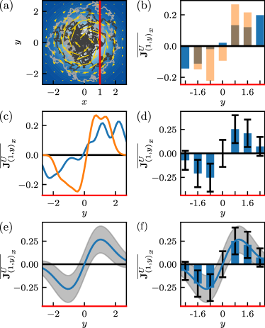
Figure 1: (a) Two trajectories (gray) with length $t=5$ in harmonically confined rotational flow Eq. (2) with $\Omega=5$. The steady-state density and current are depicted by the color gradient and yellow arrows, respectively. (b) Height of bins depict the time-averaged $x$-component of the current with Gaussian coarse-graining window Eq. (3) with $h=0.3$ evaluated for several points on the red line in (a) for the two trajectories in (a). This corresponds to time-averaging all local displacements (weighted by $U^{h}_{\mathbf{x}}$) within a single trajectory. (c) As in (b) but for the continuum of points on the red line in (a). This can be considered as the $x$-component of the current smoothened over a scale $h$. (d) Mean value $\left\langle{A}\right\rangle_{\rm s}$ and standard deviation $\sqrt{\rm var(A)}$ of $A=\overline{\mathbf{J}^{U}_{(1,y)}}_{x}$ obtained from our result Eq. (52). This represents the statistics of many histograms as in (b). (e) As in (d) but for continuous $y$ as in (c). (f) Overlaying (d) and (e) shows that the histogram picture is fully contained in the continuous coarse graining procedure.

The interpretation of the coarse graining captured in or induced by $U^{h}_{\mathbf{x}}$ in Eq. (1) is flexible; it can represent a projection or a “generalized current” [52, 53, 5, 54, 55, 15, 68, 69, 56] or may be thought of as a spatial smoothing of the empirical current and density as shown in Fig. 1c,e and Fig. 2, also for the case of a finite experimental resolution. Our main focus here is the smoothing aspect in the context of uncertainty of $p_{\rm s}(\mathbf{x}),{\mathbf{j}}_{\rm s}(\mathbf{x})$ and steady-state dissipation from individual trajectories. Note that some form of coarse graining or smoothing is in fact required in order for the quantities in Eq. (1) to be well defined [58]. A suitable smoothing decreases the uncertainty of the estimate and, if varied over sufficiently many $h$ and $\mathbf{x}$ (see also Fig. 1c,e) instead of simply ”binning”, one does not necessarily lose information (as compared to input data). Moreover, a systematic variation of the scale $h$ may reveal more information about $\overline{\rho^{U}_{\mathbf{x}}}(t)$ and $\overline{\mathbf{J}^{U}_{\mathbf{x}}}(t)$. The same reasoning is found to apply to generalized thermodynamic currents and allows for an improved inference of dissipation, see [58] and below.

The present work is an extended exposé of the conceptual and technical background that is required to understand and materialize the above observations. It accompanies the letter [58] but does not duplicate any information. Several additional explanations, illustrations and applications are given here.

The article is structured as follows. In Sec. II we lay out the theoretical background on stochastic differential equations in the Itô, Stratonovich and anti-Itô interpretations and the corresponding equations for the probability densities. We furthermore decompose the drift and steady-state current into conservative and non-conservative (i.e. irreversible) contributions and introduce dissipation. In Sec. III we prove a generalize time-reversal symmetry called “dual-reversal symmetry”. In Sec. IV we derive our main results for the steady-state (co)variances of $\overline{\rho^{U}_{\mathbf{x}}}(t)$ and $\overline{\mathbf{J}^{U}_{\mathbf{x}}}(t)$ and interpret them in terms of initial- and end-point currents and increments. We then use these results to explicitly evaluate the limit $h\to 0$ of no coarse graining in Sec. V, where we find that fluctuations diverge in $d\geq 2$-dimensional space. In Sec. VI we use current fluctuations to infer steady-state dissipation via the Thermodynamic Uncertainty Relation (TUR) [34, 15] with an emphasis on the importance of the coarse-graining scale $h$. In particular we demonstrate and explain the existence of a thermodynamically optimal coarse graining. In Sec. VII we discuss symmetries obeyed by the (co)variances and explain how the results simplify in thermodynamic equilibrium, and in Sec. VIII we present a continuity equation for coarse grained empirical densities and currents. In Sec. IX we present asymptotic results for short and long trajectories and give results for the central-limit regime. We conclude with an outlook beyond overdamped dynamics in Sec. X by considering underdamped systems as well as experimental data derived from particle-tracking experiments in biological cells, and with a summary and perspectives for the future.

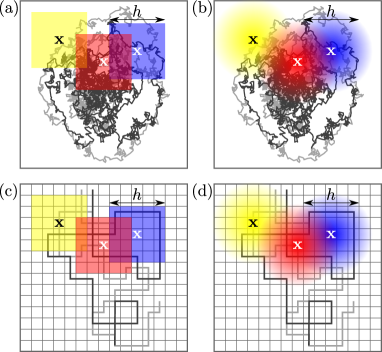
Figure 2: (a) Coarse-graining windows (colors) in the form of an indicator function of a rectangle centered at different points $\mathbf{x}$ with coarse-graining scale $h$. For each $\mathbf{x}$ and $h$, each trajectory (gray lines) gives rise to one value for the (coarse grained) time-averaged density and current. Note that the choice of $\mathbf{x}$ and $h$ is flexible such that the windows may overlap. (b) Same as (a) but with Gaussian coarse-graining windows. (c-d) Coarse-graining windows in the case of trajectory data with a finite experimental resolution (grid, gray trajectories). The coarse graining scale $h$ should be chosen large compared to the resolution to obtain reliable approximations of the (coarse-grained) densities and currents.

II Theory

II.1 Set-up – overdamped Langevin dynamics

In this section we provide background on the equations of motion for the coordinate $\mathbf{x}_{\tau}$ highlighting the differences between the Itô, Stratonovich, and anti-Itô interpretations, and for their corresponding conditional probability density functions of a transition $\mathbf{x}_{0}\to\mathbf{x}$.

We consider time-homogeneous (i.e. coefficients do not explicitly depend on time) overdamped Langevin dynamics in $d$-dimensional space with (possibly) multiplicative noise [70, 71] described by the thermodynamically consistent [20, 72] anti-Itô (or Hänggi-Klimontovich [73, 74]) stochastic differential equation

$$d\mathbf{x}_{\tau}=\mathbf{F}(\mathbf{x}_{\tau})d\tau+\bm{\sigma}(\mathbf{x}_{\tau})\circledast d\mathbf{W}_{\tau},$$ (4)

where $d\mathbf{W}_{\tau}$ is the increment of a $d$-dimensional Wiener processes (i.e. white noise) with zero mean and covariance $\langle dW_{\tau,i}dW_{\tau^{\prime},j}\rangle=\delta(\tau-\tau^{\prime})\delta_{ij}d\tau$. The noise amplitude is related to the diffusion coefficient via $\mathbf{D}(\mathbf{x})\equiv\bm{\sigma}(\mathbf{x})\bm{\sigma}(\mathbf{x})^{T}/2$. We assume the drift field $\mathbf{F}(\mathbf{x})$ to be smooth and sufficiently confining, such that the anti-Itô (end-point) convention $\circledast d\mathbf{W}_{\tau}=\mathbf{W}_{\tau}-\mathbf{W}_{\tau-d\tau}$ guarantees the existence of a steady-state probability density $p_{\rm s}(\mathbf{x})=\mathrm{e}^{-\phi(\mathbf{x})}$ and steady-state current ${\mathbf{j}}_{\rm s}(\mathbf{x})$, and yields the thermodynamically consistent Boltzmann-Gibbs (equilibrium) statistics when $\mathbf{D}(\mathbf{x})^{-1}\mathbf{F}(\mathbf{x})=-\nabla\phi(\mathbf{x})$ is a potential force.

The anti-Itô equation (4) can equivalently be rewritten as an Itô equation with an adapted drift as,

$$d\mathbf{x}_{t} =\mathbf{F}(\mathbf{x}_{t})dt+\bm{\sigma}(\mathbf{x}_{t})\circledast d\mathbf{W}_{t}$$

$$=\mathbf{F}(\mathbf{x}_{t})dt+\left[\left\{\nabla^{T}\sqrt{2\mathbf{D}(\mathbf{x}_{t})}\right\}d\mathbf{x}_{t}\right]\cdot d\mathbf{W}_{t}$$

$$\quad+\sqrt{2\mathbf{D}(\mathbf{x}_{t})}d\mathbf{W}_{t}$$

$$=\left[\mathbf{F}(\mathbf{x}_{t})+\left\{\nabla^{T}\mathbf{D}\right\}(\mathbf{x}_{t})\right]dt+\sqrt{2\mathbf{D}(\mathbf{x}_{t})}d\mathbf{W}_{t},$$ (5)

where the brackets $\{\cdot\}$ throughout denote that the differential operator only acts within the bracket and $\sqrt{2\mathbf{D}(\mathbf{x}_{t})}$ represents the matrix $\bm{\sigma}(\mathbf{x}_{t})$. At this point several remarks are in order. First, the anti-Itô interpretation of the stochastic differential equation (4) as well as the Stratonovich integral in Eq. (1) are both required for thermodynamic consistency. Second, there is no difference between the interpretations of Eq. (4) if $\mathbf{D}(\mathbf{x})=\mathbf{D}$ is a constant matrix, i.e. the convention only matters for multiplicative noise. However, even in this case the Stratonovich integral in Eq. (1) is required for thermodynamic consistency of the empirical current and to use it as an estimator of ${\mathbf{j}}_{\rm s}(\mathbf{x})$.

The Fokker-Planck equation for the conditional probability density $G(\mathbf{x},t|\mathbf{y})$ to be at a point $\mathbf{x}$ at time $t$ after starting at $\mathbf{y}$ that corresponds to Eqs. (4) and (5) reads

$$\partial_{t}G(\mathbf{x},t|\mathbf{y}) =[-\nabla_{\mathbf{x}}\cdot\mathbf{F}(\mathbf{x})+\nabla_{\mathbf{x}}^{T}\mathbf{D}(\mathbf{x})\nabla_{\mathbf{x}}]G(\mathbf{x},t|\mathbf{y})$$

$$\equiv L(\mathbf{x})G(\mathbf{x},t|\mathbf{y}),$$ (6)

which satisfies a continuity equation $(\partial_{t}+\nabla_{\mathbf{x}}\cdot\hat{\mathbf{j}}_{\mathbf{x}})G(\mathbf{x},t|\mathbf{y})=0$, where

$$\hat{\mathbf{j}}_{\mathbf{x}}\equiv\mathbf{F}(\mathbf{x})-\mathbf{D}(\mathbf{x})\nabla_{\mathbf{x}}.$$ (7)

Decomposing of the drift $\mathbf{F}(\mathbf{x})$ into reversible $\mathbf{F}^{\rm rev}(\mathbf{x})=-\mathbf{D}(\mathbf{x})\{\nabla\phi\}(\mathbf{x})$ and irreversible $\mathbf{F}^{\rm irrev}(\mathbf{x})=\mathbf{F}(\mathbf{x})-\mathbf{F}^{\rm rev}(\mathbf{x})$ parts translates to a decomposition of $\hat{\mathbf{j}}_{\mathbf{x}}$ into a gradient part $\hat{\mathbf{j}}^{g}(\mathbf{x})$ and steady-state-current contributions, namely $\hat{\mathbf{j}}_{\mathbf{x}}=\mathbf{F}^{\rm irrev}(\mathbf{x})+\mathbf{F}^{\rm rev}(\mathbf{x})-\mathbf{D}(\mathbf{x})\nabla_{\mathbf{x}}$. This is rewritten using

$$\hat{\mathbf{j}}^{g}(\mathbf{x}) \equiv\mathbf{F}^{\rm rev}(\mathbf{x})-\mathbf{D}(\mathbf{x})\nabla$$

$$=\mathbf{D}(\mathbf{x})\left\{\nabla\log(p_{\rm s}(\mathbf{x})\right\}-\mathbf{D}(\mathbf{x})\nabla$$

$$=\mathbf{D}(\mathbf{x})p_{\rm s}^{-1}(\mathbf{x})\left\{\nabla p_{\rm s}(\mathbf{x})\right\}-\mathbf{D}(\mathbf{x})\nabla$$

$$=-\mathbf{D}(\mathbf{x})\left[p_{\rm s}(\mathbf{x})\{\nabla p_{\rm s}^{-1}(\mathbf{x})\}-\nabla\right]$$

$$=-\mathbf{D}(\mathbf{x})p_{\rm s}(\mathbf{x})\nabla p_{\rm s}^{-1}(\mathbf{x}),$$ (8)

where we have used that ${\{\nabla p_{\rm s}(\mathbf{x})^{-1}\}}{=}{-p_{\rm s}^{-2}(\mathbf{x})\{\nabla p_{\rm s}\}(\mathbf{x})}$ implies ${\{\nabla p_{\rm s}\}(\mathbf{x})}{=}{-p_{\rm s}^{2}(\mathbf{x})\{\nabla p_{\rm s}^{-1}\}(\mathbf{x})}$). Therefore we have $\hat{\mathbf{j}}^{g}(\mathbf{x})p_{\rm s}(\mathbf{x})=0$, such that the definition of the steady-state current ${\mathbf{j}}_{\rm s}(\mathbf{x})\equiv\hat{\mathbf{j}}(\mathbf{x})p_{\rm s}(\mathbf{x})$ with $\hat{\mathbf{j}}_{\mathbf{x}}=\hat{\mathbf{j}}^{g}(\mathbf{x})+\mathbf{F}^{\rm irrev}(\mathbf{x})$ implies $\mathbf{F}^{\rm irrev}(\mathbf{x})=p_{\rm s}^{-1}(\mathbf{x}){\mathbf{j}}_{\rm s}(\mathbf{x})$ and we obtain

$$\hat{\mathbf{j}}_{\mathbf{x}} =\hat{\mathbf{j}}^{g}_{\mathbf{x}}+p_{\rm s}^{-1}(\mathbf{x}){\mathbf{j}}_{\rm s}(\mathbf{x})$$

$$=-p_{\rm s}(\mathbf{x})\mathbf{D}(\mathbf{x})\nabla_{\mathbf{x}}p_{\rm s}^{-1}(\mathbf{x})+p_{\rm s}^{-1}(\mathbf{x}){\mathbf{j}}_{\rm s}(\mathbf{x}).$$ (9)

Moreover, note that the steady-state two-point density $P_{\mathbf{y}}(\mathbf{x},t)\equiv G(\mathbf{x},t|\mathbf{y})p_{\rm s}(\mathbf{y})$ also satisfies the same Fokker-Planck equation as $G(\mathbf{x},t|\mathbf{y})$.

Finally, if the process is irreversible, i.e. $\mathbf{F}^{\rm irrev}(\mathbf{x})\neq\mathbf{0}$ the steady state is dissipative with an average total entropy production rate $\dot{\Sigma}$ given by [75, 21]

$$\dot{\Sigma} =\int d\mathbf{x}\mathbf{F}^{\rm irrev}(\mathbf{x})\cdot\mathbf{D}^{-1}(\mathbf{x})\mathbf{F}^{\rm irrev}(\mathbf{x})p_{\rm s}(\mathbf{x})$$

$$=\int d\mathbf{x}\frac{{\mathbf{j}}_{\rm s}^{T}(\mathbf{x})}{p_{\rm s}(\mathbf{x})}\mathbf{D}^{-1}(\mathbf{x}){\mathbf{j}}_{\rm s}(\mathbf{x}),$$ (10)

which can be obtained as the mean value of a sum over steady-state expectations of the respective $i$-th component of $\overline{\mathbf{J}^{U_{i}}_{\mathbf{x}}}(t)$ in Eq. (1) with $U_{i}=(\mathbf{F}^{\rm irrev}(\mathbf{x})^{T}\mathbf{D}^{-1}(\mathbf{x}))_{i}$.

Note that by adopting the Itô or Stratonovich conventions instead of the anti-Itô convention in Eq. (4) one obtains a different Fokker-Planck equation with a different steady-state density. In particular, $L^{\rm Ito}(\mathbf{x})=-\nabla_{\mathbf{x}}\cdot\mathbf{F}(\mathbf{x})+\sum_{i,j=1}^{d}\partial_{i}\partial_{j}D_{ij}(\mathbf{x})$ and $L^{\rm Strato}(\mathbf{x})=L(\mathbf{x})/2+L^{\rm Ito}(\mathbf{x})/2=-\nabla_{\mathbf{x}}\cdot\mathbf{F}(\mathbf{x})+\sum_{i,j=1}^{d}\partial_{i}\sqrt{D_{ij}(\mathbf{x})}\partial_{j}\sqrt{D_{ij}(\mathbf{x})}$ and the respective steady-state densities $p_{\rm s}^{\rm Ito}(\mathbf{x})$ and $p_{\rm s}^{\rm Strato}(\mathbf{x})$ depend explicitly on $\mathbf{D}(\mathbf{x})$ and are therefore in general not thermodynamically consistent since the steady state deviates from Gibbs-Boltzmann statistics (e.g. in dimension one we have $p_{\rm s}^{\rm Ito}(x)\propto p_{\rm s}^{\textrm{anti-Ito}}(x)/D(x)$ and $p_{\rm s}^{\rm Strato}(x)\propto p_{\rm s}^{\textrm{anti-Ito}}(x)/\sqrt{D(x)}$, respectively, where the deviation from $p_{\rm s}^{\textrm{anti-Ito}}(x)$ cannot be absorbed in the normalization if $D(x)$ depends on $x$).

III Generalized time-reversal symmetry

It will later prove useful to take into account a form of generalized time-reversal symmetry obeyed by Eq. (4) called “continuous time reversal” or “dual-reversal symmetry” [76, 55]. Analogous generalized symmetries were also found in deterministic systems (see e.g. [77]). Generalized time-reversal symmetry relates forward dynamics in non-equilibrium steady states to time-reversed dynamics in an ensemble with inverted irreversible steady-state current, i.e. in an ensemble with $\mathbf{F}^{\rm irrev}\to-\mathbf{F}^{\rm irrev}$ or equivalently ${\mathbf{j}}_{\rm s}\to-{\mathbf{j}}_{\rm s}$. The dual-reversal symmetry for the two-point probability densities states that

$$G(\mathbf{x},t|\mathbf{y})p_{\rm s}(\mathbf{y})=G^{-{\mathbf{j}}_{\rm s}}(\mathbf{y},t|\mathbf{x})p_{\rm s}(\mathbf{x}),$$ (11)

or equivalently $G^{-{\mathbf{j}}_{\rm s}}(\mathbf{x},t|\mathbf{y})p_{\rm s}(\mathbf{y})=G(\mathbf{y},t|\mathbf{x})p_{\rm s}(\mathbf{x})$ where $G^{-{\mathbf{j}}_{\rm s}}(\mathbf{y},t|\mathbf{x})$ is the conditional probability density of the process with drift $\mathbf{F}^{-{\mathbf{j}}_{\rm s}}(\mathbf{x})\equiv\mathbf{F}^{\rm rev}(\mathbf{x})-\mathbf{F}^{\rm irrev}(\mathbf{x})$ instead of $\mathbf{F}(\mathbf{x})=\mathbf{F}^{\rm rev}(\mathbf{x})+\mathbf{F}^{\rm irrev}(\mathbf{x})$. At equilibrium, i.e. ${\mathbf{j}}_{\rm s}(\mathbf{x})=\mathbf{0}$ (for all $\mathbf{x}$), this symmetry simplifies to the well known time-reversal symmetry called “detailed balance” condition for two-point densities. We here provide an original and intuitive proof of Eq. (11) that proceeds entirely in continuous space and time, based on the decomposition of currents Eq. (9). The Fokker-Planck operator $L(\mathbf{x})=-\nabla_{\mathbf{x}}\cdot\hat{\mathbf{j}}_{\mathbf{x}}$, using the decomposition Eq. (9) and multiplying by $p_{\rm s}$ from the right side, reads

$$L(\mathbf{x})p_{\rm s}(\mathbf{x})=-\nabla_{\mathbf{x}}\cdot{\mathbf{j}}_{\rm s}(\mathbf{x})+\nabla_{\mathbf{x}}^{T}p_{\rm s}(\mathbf{x})\mathbf{D}(\mathbf{x})\nabla_{\mathbf{x}}.$$ (12)

Taking the adjoint gives (since $\mathbf{D}=\mathbf{D}^{T}$)

$$p_{\rm s}(\mathbf{x})L^{\dagger}(\mathbf{x}) =[L(\mathbf{x})p_{\rm s}(\mathbf{x})]^{\dagger}$$

$$={\mathbf{j}}_{\rm s}(\mathbf{x})\cdot\nabla_{\mathbf{x}}+\nabla_{\mathbf{x}}^{T}p_{\rm s}(\mathbf{x})\mathbf{D}(\mathbf{x})\nabla_{\mathbf{x}}.$$ (13)

Since for the steady state density $Lp_{\rm s}=0$, ${\mathbf{j}}_{\rm s}$ is divergence free $\{\nabla_{\mathbf{x}}\cdot{\mathbf{j}}_{\rm s}(\mathbf{x})\}=0$ and we have $\nabla_{\mathbf{x}}\cdot{\mathbf{j}}_{\rm s}(\mathbf{x})={\mathbf{j}}_{\rm s}(\mathbf{x})\cdot\nabla_{\mathbf{x}}$. Thus we see the symmetry under inversion ${\mathbf{j}}_{\rm s}\rightarrow-{\mathbf{j}}_{\rm s}$

$$p_{\rm s}(\mathbf{x})L^{\dagger}(\mathbf{x})=L^{-{\mathbf{j}}_{\rm s}}(\mathbf{x})p_{\rm s}(\mathbf{x}).$$ (14)

Under detailed balance ${\mathbf{j}}_{\rm s}=\mathbf{0}$, i.e. $L^{-{\mathbf{j}}_{\rm s}}=L$, and $p_{\rm s}(\mathbf{x})L^{\dagger}(\mathbf{x})=L(\mathbf{x})p_{\rm s}(\mathbf{x})$ which implies the time-reversal symmetry $G(\mathbf{x},t|\mathbf{y})p_{\rm s}(\mathbf{y})=G(\mathbf{y},t|\mathbf{x})p_{\rm s}(\mathbf{x})$ [78, 71, 59]. Eq. (14) implies for all integers $n\geq 1$ that $p_{\rm s}(\mathbf{x})[L^{\dagger}(\mathbf{x})]^{n}=[L(\mathbf{x})^{-{\mathbf{j}}_{\rm s}}]^{n}(\mathbf{x})p_{\rm s}(\mathbf{x})$, and consequently for all $t\geq 0$ that $p_{\rm s}(\mathbf{x})\exp[L^{\dagger}(\mathbf{x})t]=\exp[L^{-{\mathbf{j}}_{\rm s}}(\mathbf{x})t]p_{\rm s}(\mathbf{x})$. Applying this operator equation to the initial condition $\delta(\mathbf{y}-\mathbf{x})$ and using $p_{\rm s}(\mathbf{x})\delta(\mathbf{y}-\mathbf{x})=p_{\rm s}(\mathbf{y})\delta(\mathbf{y}-\mathbf{x})$ as well as that $L^{\dagger}$ propagates the initial condition as $G(\mathbf{y},t|\mathbf{x})=\exp[L^{\dagger}(\mathbf{x})t]\delta(\mathbf{y}-\mathbf{x})$ while $L^{-{\mathbf{j}}_{\rm s}}$ propagates the final point in the ensemble with ${\mathbf{j}}_{\rm s}$ inverted $G^{-{\mathbf{j}}_{\rm s}}(\mathbf{x},t|\mathbf{y})=\exp[L^{-{\mathbf{j}}_{\rm s}}(\mathbf{x})t]\delta(\mathbf{y}-\mathbf{x})$, we obtain the dual reversal symmetry in Eq. (11). This generalized time-reversal symmetry relates the dynamics in the time-reversed ensemble to the propagation in the ensemble with reversed current, or equivalently, the forward dynamics to the propagation with concurrent time and ${\mathbf{j}}_{\rm s}$-reversal. While at equilibrium (i.e. under detailed balance, ${\mathbf{j}}_{\rm s}=\mathbf{0}$) the forward dynamics is indistinguishable from the time-reversed dynamics, the statement Eq. (11) (if generalized to all paths (see e.g. [55]) means that forward dynamics (with ${\mathbf{j}}_{\rm s}$) is indistinguishable from backwards/time-reversed dynamics with reversed ${\mathbf{j}}_{\rm s}\to-{\mathbf{j}}_{\rm s}$ (i.e. ${\mathbf{j}}_{\rm s}(\mathbf{x})\to-{\mathbf{j}}_{\rm s}(\mathbf{x})$ at all $\mathbf{x}$). We will later use this dual-reversal symmetry to understand the fluctuations of observables that involve (time-integrated) currents in non-equilibrium steady states.

IV Derivation of the main results, initial- and final-point currents and their application to density-current correlations

IV.1 Mean empirical density and current

Although the time-averaged density and current defined in Eq. (1) are functionals with complicated statistics, their mean values can be readily computed. Throughout the paper we will assume steady-state initial conditions, i.e. initial conditions drawn from $p_{\rm s}(\mathbf{x}^{\prime})$, denoted by $\left\langle{\cdot}\right\rangle_{\rm s}$. This renders mean values time-independent and we have (see also [6])

$$\left\langle{\overline{\rho^{U}_{\mathbf{x}}}(t)}\right\rangle_{\rm s} =\frac{1}{t}\int_{0}^{t}d\tau\left\langle{U^{h}_{\mathbf{x}}(\mathbf{x}_{\tau})}\right\rangle_{\rm s}$$

$$=\frac{1}{t}\int_{0}^{t}d\tau\int d\mathbf{z}U^{h}_{\mathbf{x}}(\mathbf{z})p_{\rm s}(\mathbf{z})$$

$$=\int d\mathbf{z}U^{h}_{\mathbf{x}}(\mathbf{z})p_{\rm s}(\mathbf{z}),$$ (15)

and by rewriting the Stratonovich-integration $\circ d\mathbf{x}_{\tau}$ in terms of Itô integration as $U^{h}_{\mathbf{x}}(\mathbf{x}_{\tau})\circ d\mathbf{x}_{\tau}=U^{h}_{\mathbf{x}}(\mathbf{x}_{\tau})d\mathbf{x}_{\tau}+\frac{1}{2}dU^{h}_{\mathbf{x}}(\mathbf{x}_{\tau})d\mathbf{x}_{\tau}$, where $d\mathbf{x}_{\tau}d\mathbf{x}_{\tau}^{T}/2=\mathbf{D}(\mathbf{x}_{\tau})d\tau$ and thus $dU^{h}_{\mathbf{x}}(\mathbf{x}_{\tau})d\mathbf{x}_{\tau}/2=\mathbf{D}(\mathbf{x}_{\tau})\{\nabla U^{h}_{\mathbf{x}}\}(\mathbf{x}_{\tau})d\tau$,

$$\left\langle{\overline{\mathbf{J}^{U}_{\mathbf{x}}}(t)}\right\rangle_{\rm s}=\frac{1}{t}\int_{0}^{t}\left\langle{U^{h}_{\mathbf{x}}(\mathbf{x}_{\tau})\circ d\mathbf{x}_{\tau}}\right\rangle_{\rm s}$$

$$=\frac{1}{t}\int_{\tau=0}^{\tau=t}\left\langle{U^{h}_{\mathbf{x}}(\mathbf{x}_{\tau})d\mathbf{x}_{\tau}}\right\rangle_{\rm s}+\frac{1}{t}\int_{\tau=0}^{\tau=t}\frac{1}{2}\left\langle{dU^{h}_{\mathbf{x}}(\mathbf{x}_{\tau})d\mathbf{x}_{\tau}}\right\rangle_{\rm s}$$

$$=\frac{1}{t}\int_{0}^{t}d\tau\int d\mathbf{z}p_{\rm s}(\mathbf{z})\big{[}U^{h}_{\mathbf{x}}(\mathbf{z})\mathbf{F}(\mathbf{z})+\left\{\nabla^{T}_{\mathbf{z}}\mathbf{D}(\mathbf{z})\right\}U^{h}_{\mathbf{x}}(\mathbf{z})$$

$$+\mathbf{D}(\mathbf{z})\left\{\nabla_{\mathbf{z}}U^{h}_{\mathbf{x}}(\mathbf{z})\right\}\big{]}+\frac{1}{t}\int_{\tau=0}^{\tau=t}\left\langle{U^{h}_{\mathbf{x}}(\mathbf{x}_{\tau})\sqrt{2\mathbf{D}(\mathbf{x}_{\tau})}d\mathbf{W}_{\tau}}\right\rangle_{\rm s}.$$ (16)

Note that the mean value involving $d\mathbf{W}_{\tau}$ vanishes since this Itô-noise increment has zero mean and is uncorrelated with functions of $\mathbf{x}_{\tau}$, i.e. $\langle f(\mathbf{x}_{\tau})d\mathbf{W}_{\tau}\rangle=\langle f(\mathbf{x}_{\tau})\rangle\langle d\mathbf{W}_{\tau}\rangle=0$. Integrating by parts and using that $\mathbf{D}(\mathbf{z})=\mathbf{D}^{T}(\mathbf{z})$ is symmetric we get

$$\left\langle{\overline{\mathbf{J}^{U}_{\mathbf{x}}}(t)}\right\rangle_{\rm s} =\int d\mathbf{z}p_{\rm s}(\mathbf{z})\left[U^{h}_{\mathbf{x}}(\mathbf{z})\mathbf{F}(\mathbf{z})+\nabla^{T}_{\mathbf{z}}\mathbf{D}(\mathbf{z})U^{h}_{\mathbf{x}}(\mathbf{z})\right]$$

$$=\int d\mathbf{z}U^{h}_{\mathbf{x}}(\mathbf{z})\left[\mathbf{F}(\mathbf{z})-\mathbf{D}(\mathbf{z})\nabla_{\mathbf{z}}\right]p_{\rm s}(\mathbf{z})$$

$$=\int d\mathbf{z}U^{h}_{\mathbf{x}}(\mathbf{z})\hat{\mathbf{j}}_{\mathbf{z}}p_{\rm s}(\mathbf{z})=\int d\mathbf{z}U^{h}_{\mathbf{x}}(\mathbf{z}){\mathbf{j}}_{\rm s}(\mathbf{z}).$$ (17)

Note that if we had defined Eq. (1) with an Itô integral instead of the Stratonovich, we would miss the $\mathbf{D}(\mathbf{z})\nabla_{\mathbf{z}}$-term and would not get $\hat{\mathbf{j}}_{\mathbf{z}}$ and thus ${\mathbf{j}}_{\rm s}$, not even for additive noise. The Stratonovich integral is therefore required for consistency.

The interpretation of the steady-state mean values in Eqs. (15) and (17) is immediate — the mean time-averaged density and current are (at least for positive normalized windows) the steady-state density $p_{\rm s}$ and current ${\mathbf{j}}_{\rm s}$ averaged over the coarse-graining window function $U^{h}_{\mathbf{x}}$.

IV.2 (Co)variances of empirical density and current

Since fluctuations [34, 15, 50, 51, 52, 53, 5, 54, 55] (and correlations [56]) play a crucial role in time-average statistical mechanics and stochastic thermodynamics, we discuss (co)variances of coarse-grained time-averaged densities and currents (recall the interpretation of the variance within the “fluctuating histogram” picture in Fig. 1).

To keep the notation tractable we introduce the integral operator

$$\!\hat{\mathcal{I}}^{t,U}_{\mathbf{x}\mathbf{y}}[\,\cdot\,]\equiv\frac{1}{t^{2}}\!\int_{0}^{t}\!dt_{1}\!\!\int_{t_{1}}^{t}\!dt_{2}\!\!\int\!d\mathbf{z}U^{h}_{\mathbf{x}}(\mathbf{z})\!\!\int\!d\mathbf{z}^{\prime}U^{h}_{\mathbf{y}}(\mathbf{z}^{\prime})[\,\cdot\,],$$ (18)

with the convention $\int_{t_{1}}^{t}dt_{2}\delta(t_{2}-t_{1})=1/2$. Note that other conventions would only change the appearance of intermediate steps but not the final result. We define the two-point steady-state covariance according to [58] as

$$C^{\mathbf{x}\mathbf{y}}_{AB}(t)\equiv\langle A_{\mathbf{x}}(t)B_{\mathbf{y}}(t)\rangle_{\rm s}-\langle A_{\mathbf{x}}(t)\rangle_{\rm s}\langle B_{\mathbf{y}}(t)\rangle_{\rm s}\,,$$ (19)

where $A$ and $B$ are henceforth either $\overline{\rho^{U}}$ or $\overline{\mathbf{J}^{U}}$, respectively. We refer to the case when $A\neq B$ or $\mathbf{x}\neq\mathbf{y}$ as (linear) “correlations” and to the case $A=B$ with $\mathbf{x}=\mathbf{y}$ as “fluctuations” whereby we adopt the convention ${\mathrm{var}^{\mathbf{x}}_{A}(t)\equiv C^{\mathbf{x}\mathbf{x}}_{AA}(t)}$. Note that for simplicity and enhanced readability we only assume coarse-graining windows $U^{h}_{\mathbf{x}}$ and $U^{h}_{\mathbf{y}}$ where the shape is fixed but the center points $\mathbf{x},\mathbf{y}$ may differ. All results equivalently hold for window functions whose shape and $h$ differs as well.

We now address correlations $C^{\mathbf{x}\mathbf{y}}_{\rho\rho}$ of the coarse-grained time-averaged density at points $\mathbf{x}$ and $\mathbf{y}$, which corresponds to the density variance when $\mathbf{x}=\mathbf{y}$. To do so, first consider the (mixed) second moment

$$\left\langle{\overline{\rho^{U}_{\mathbf{x}}}(t)\overline{\rho^{U}_{\mathbf{y}}}(t)}\right\rangle_{\rm s} =\int_{0}^{t}d\tau\int_{0}^{t}d\tau^{\prime}\left\langle{U^{h}_{\mathbf{x}}(\mathbf{x}_{\tau})U^{h}_{\mathbf{y}}(\mathbf{x}_{\tau}^{\prime})}\right\rangle_{\rm s}.$$ (20)

The expectation value corresponds to an integration over the two-point probability density to have $\mathbf{x}_{\tau}=\mathbf{z}$ and $\mathbf{x}_{\tau^{\prime}}=\mathbf{z}^{\prime}$ given by the two-point function $P_{\mathbf{z}}(\mathbf{z}^{\prime},\tau^{\prime}-\tau)\equiv G(\mathbf{z}^{\prime},\tau^{\prime}-\tau|\mathbf{z})p_{\rm s}(\mathbf{z})$ for $\tau^{\prime}>\tau$ and $P_{\mathbf{z}^{\prime}}(\mathbf{z},\tau-\tau^{\prime})$ for $\tau^{\prime}<\tau$. We relabel the times $\tau,\tau^{\prime}$ as $t_{1}<t_{2}$ and use the integral operator in Eq. (18) to obtain

$$\left\langle{\overline{\rho^{U}_{\mathbf{x}}}(t)\overline{\rho^{U}_{\mathbf{y}}}(t)}\right\rangle_{\rm s} =\hat{\mathcal{I}}^{t,U}_{\mathbf{x}\mathbf{y}}\left[P_{\mathbf{z}}(\mathbf{z}^{\prime},t_{2}-t_{1})+P_{\mathbf{z}}(\mathbf{z}^{\prime},t_{2}-t_{1})\right].$$ (21)

Since the argument only depends on time differences $t^{\prime}=t_{2}-t_{1}\geq 0$ the integral operator Eq. (18) simplifies to

$$\!\!\hat{\mathcal{I}}^{t,U}_{\mathbf{x}\mathbf{y}}[\,\cdot\,]\equiv\frac{1}{t}\!\int_{0}^{t}\!\!\!dt^{\prime}\!\left(1-\frac{t^{\prime}}{t}\right)\!\!\int\!d\mathbf{z}U^{h}_{\mathbf{x}}(\mathbf{z})\!\!\int\!\!d\mathbf{z}^{\prime}U^{h}_{\mathbf{y}}(\mathbf{z}^{\prime})[\,\cdot\,].$$ (22)

To obtain the correlation we subtract the mean values (see Eq. (15)) which (noting that $(1/t)\int_{0}^{t}dt^{\prime}(1-t^{\prime}/t)=1/2$) gives

$$\!\!C^{\mathbf{x}\mathbf{y}}_{\rho\rho}(t)=\hat{\mathcal{I}}^{t,U}_{\mathbf{x}\mathbf{y}}\left[P_{\mathbf{z}}(\mathbf{z}^{\prime},t^{\prime})+P_{\mathbf{z}^{\prime}}(\mathbf{z},t^{\prime})-2p_{\rm s}(\mathbf{z})p_{\rm s}(\mathbf{z}^{\prime})\right],$$ (23)

which has been derived before [79, 51]. Eq. (23) simplifies further for $\mathbf{x}=\mathbf{y}$ as well as under detailed balance and is also symmetric under ${\mathbf{j}}_{\rm s}\to-{\mathbf{j}}_{\rm s}$, all of which will be discussed in Sec. VII.

The interpretation of Eq. (23) (see also [51]) is that all paths from $\mathbf{z}$ to $\mathbf{z}^{\prime}$ (i.e. from $U^{h}_{\mathbf{x}}$ to $U^{h}_{\mathbf{y}}$) and vice versa from $\mathbf{z}^{\prime}$ to $\mathbf{z}$, in time $t^{\prime}=t_{2}-t_{1}$ contribute according to their correlation to $C^{\mathbf{x}\mathbf{y}}_{\rho\rho}(t)$. These contributions are integrated over all possible time differences and pairs of points within $U^{h}_{\mathbf{x}}$ and $U^{h}_{\mathbf{y}}$, respectively.

We now explore the important effect of coarse graining over the windows $U^{h}_{\mathbf{x}}$ for the inference of $p_{\rm s}(\mathbf{x})$ from noisy individual trajectories. If one wants to reliably infer the (coarse-grained) steady-state density from $\overline{\rho^{U}_{\mathbf{x}}}(t)$ the relative error ${\rm var}_{\rho}/\langle\overline{\rho^{U}_{\mathbf{x}}}(t)\rangle^{2}$ should be small. We have shown that $\lim_{h\to 0}{\rm var}_{\rho}/\langle\overline{\rho^{U}_{\mathbf{x}}}(t)\rangle^{2}=\infty$ [58] and Fig. 3 (blue line) demonstrates that ${\rm var}_{\rho}/\langle\overline{\rho^{U}_{\mathbf{x}}}(t)\rangle^{2}$ decreases with increasing $h$. However, such a decrease does not guarantee an improved inference. Namely, as $h\to\infty$ the time to spent in the region around $\mathbf{x}$ tends to $t$ and $U^{h}_{\mathbf{x}}$ becomes constant on a large region and hence $\overline{\rho^{U}_{\mathbf{x}}}(t)\to U^{h}_{\mathbf{x}}(\mathbf{x})$ which contains no information about $p_{\rm s}(\mathbf{x})$. Therefore, to reliably infer that $\overline{\rho^{U}_{\mathbf{x}}}$ significantly deviates from $U^{h}_{\mathbf{x}}(\mathbf{x})$ we must also consider the relative error of $[\overline{\rho^{U}_{\mathbf{x}}}-U^{h}_{\mathbf{x}}(\mathbf{x})]$ depicted in Fig. 3 (orange line). There exists an ”optimal coarse graining” where the uncertainty of simultaneously inferring $\overline{\rho^{U}_{\mathbf{x}}}$ and $\overline{\rho^{U}_{\mathbf{x}}}-U^{h}_{\mathbf{x}}(\mathbf{x})$ is minimal (minimum of the solid lines in Fig. 3) which represents the most reliable and informative estimate of $\overline{\rho^{U}_{\mathbf{x}}}$. In Sec. VI we will turn to an analogous “optimal coarse graining” with respect to current variances and a system’s dissipation.

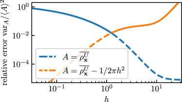
Figure 3: Relative error of $\overline{\rho^{U}_{\mathbf{x}}}(t)$ (blue line) compared to the relative error of $[\overline{\rho^{U}_{\mathbf{x}}}(t)-U^{h}_{\mathbf{x}}(\mathbf{x})]$ (orange line) as a function of the coarsening scale $h$ for the rotational flow Eq. (2) with $\Omega=3$ for time $t=10$ with a Gaussian window function Eq. (3) around $\mathbf{x}=(1,0)^{T}$ with width $h$, i.e. $U^{h}_{\mathbf{x}}(\mathbf{x})=(2\pi h^{2})^{-1}$. The intersection point of blue and orange lines at $h\approx 1.3$ yields an ”optimal coarse graining” where the maximum of the two lines (solid line) is minimal, whereas the maximum of the relative errors diverges as $h\to\infty$ since $\left\langle{A}\right\rangle_{\rm s}\to 0$ and diverges logarithmically for $h\to 0$ (as we will see in Eq. (51)).

We now consider coarse-grained time-averaged currents. To compute the correlation of the current at a point $\mathbf{x}$ and the density at $\mathbf{y}$ we need to consider

$$\left\langle{\overline{\mathbf{J}^{U}_{\mathbf{x}}}(t)\overline{\rho^{U}_{\mathbf{y}}}(t)}\right\rangle_{\rm s} =\int_{0}^{t}d\tau\int_{\tau^{\prime}=0}^{\tau^{\prime}=t}\left\langle{U^{h}_{\mathbf{x}}(\mathbf{x}_{\tau})U^{h}_{\mathbf{y}}(\mathbf{x}_{\tau}^{\prime})\circ d\mathbf{x}_{\tau^{\prime}}}\right\rangle_{\rm s}.$$ (24)

Relabeling with $t_{1}\leq t_{2}$, introducing the notation

$$\left\langle{\cdots}\right\rangle^{\mathbf{x}_{t_{1}}=\mathbf{z}}_{\mathbf{x}_{t_{2}}=\mathbf{z}^{\prime}}\equiv\left\langle{\delta(\mathbf{x}_{t_{1}}-\mathbf{z})\delta(\mathbf{x}_{t_{2}}-\mathbf{z}^{\prime})\cdots}\right\rangle_{\rm s},$$ (25)

and considering the Stratonovich increments

$$\circ d\mathbf{x}_{\tau}\equiv\mathbf{x}_{\tau+d\tau/2}-\mathbf{x}_{\tau-d\tau/2},$$ (26)

and subtracting the mean values (15) and (17), we can write the correlation as

$$\mathbf{C}^{\mathbf{x}\mathbf{y}}_{\mathbf{J}\rho}(t)=\hat{\mathcal{I}}^{t,U}_{\mathbf{x}\mathbf{y}} \Bigg{[}\frac{{\left\langle{\circ d\mathbf{x}_{t_{1}}}\right\rangle}^{\mathbf{x}_{t_{2}}=\mathbf{z}^{\prime}}_{\mathbf{x}_{t_{1}}=\mathbf{z}}}{dt_{1}}$$

$$+\frac{{\left\langle{\circ d\mathbf{x}_{t_{2}}}\right\rangle}^{\mathbf{x}_{t_{2}}=\mathbf{z}}_{\mathbf{x}_{t_{1}}=\mathbf{z}^{\prime}}}{dt_{2}}-2{\mathbf{j}}_{\rm s}(\mathbf{z})p_{\rm s}(\mathbf{z}^{\prime})\Bigg{]}.$$ (27)

Eq. (27) is harder to compute and more difficult to interpret as compared to $C^{\mathbf{x}\mathbf{y}}_{\rho\rho}(t)$ (see Eq. (23)). The quantities involving Stratonovich increments characterize the mean initial- and final displacements of “pinned” paths of duration $t_{2}-t_{1}$ conditioned on the initial and final points $\mathbf{z},\mathbf{z}^{\prime}$ or $\mathbf{z}^{\prime},\mathbf{z}$, respectively. Note that $\mathbf{z}$ always denotes the point where the increment occurs. Via the integral operator in Eq. (18) or (22) the $\mathbf{z}$ variable is integrated over $U^{h}_{\mathbf{x}}(\mathbf{z})$, i.e. in $\mathbf{C}^{\mathbf{x}\mathbf{y}}_{\mathbf{J}\rho}(t)$ the variable $\mathbf{z}$ corresponds to the window at $\mathbf{x}$ where the (coarse-grained) current is evaluated. Therefore, correlations between a current and a density depend on integrals over conditioned initial-point increments at a point $\mathbf{z}$ at time $t_{1}$, and conditioned final-point increments, also at $\mathbf{z}$, at time $t_{2}>t_{1}$. We define the increments divided by $dt_{i}$ to be the ”initial- and final-point currents”,

$$\mathbf{j}_{\rm in}(\mathbf{z}^{\prime},t_{2}-t_{1};\mathbf{z}) \equiv\frac{\left\langle{\circ d\mathbf{x}_{t_{1}}}\right\rangle^{\mathbf{x}_{t_{2}}=\mathbf{z}^{\prime}}_{\mathbf{x}_{t_{1}}=\mathbf{z}}}{dt_{1}}$$

$$\mathbf{j}_{\rm fi}(\mathbf{z},t_{2}-t_{1};\mathbf{z}^{\prime}) \equiv\frac{\left\langle{\circ d\mathbf{x}_{t_{2}}}\right\rangle^{\mathbf{x}_{t_{2}}=\mathbf{z}}_{\mathbf{x}_{t_{1}}=\mathbf{z}^{\prime}}}{dt_{2}}.$$ (28)

In order to understand the correlation in Eq. (27) we must therefore understand initial- and final-point currents. This is a priori not easy, since initial-point currents involve both, spatial increments at $t_{1}$ and probabilities of reaching a final point at time $t_{2}>t_{1}$, which involves non-trivial correlations — a given displacement affects (and thus correlates with) the probability to reach the final point. We will derive a statement (“Lemma”) in the next subsection that solves all mathematical difficulties related to this issue, without resorting to Feynman-Kac and path-integral methods as in Ref. [80]. Then we will make intuitive sense of the result by exploiting the dual-reversal symmetry in Eq. (11).

Before doing so, we also consider the scalar current-current covariance $C^{\mathbf{x}\mathbf{y}}_{\mathbf{J}\cdot\mathbf{J}}(t)$ (note that the complete fluctuations and correlations of $\overline{\mathbf{J}^{U}_{\mathbf{x}}}(t)$ are characterized by the $d\times d$ covariance matrix with elements $(\mathsf{C}^{\mathbf{x}\mathbf{y}}_{\mathbf{J}\mathbf{J}}(t))_{ik}=C^{\mathbf{x}\mathbf{y}}_{{\rm J}_{i}{\rm J}_{k}}(t)$; here we focus on the scalar case $C^{\mathbf{x}\mathbf{y}}_{\mathbf{J}\cdot\mathbf{J}}(t)\equiv\mathrm{Tr}\mathsf{C}^{\mathbf{x}\mathbf{y}}_{\mathbf{J}\mathbf{J}}(t)$). Notably, almost all results remain completely equivalent for other elements of the covariance matrix, scalar products simply have a slightly more intuitive geometrical interpretation and notation. Writing down the definition and using the notations as in the steps towards Eq. (27) we immediately arrive at

$$C^{\mathbf{x}\mathbf{y}}_{\mathbf{J}\cdot\mathbf{J}}(t)= \hat{\mathcal{I}}^{t,U}_{\mathbf{x}\mathbf{y}}\Bigg{[}\frac{{\left\langle{\circ d\mathbf{x}_{t_{1}}\cdot\circ d\mathbf{x}_{t_{2}}}\right\rangle}^{\mathbf{x}_{t_{2}}=\mathbf{z}^{\prime}}_{\mathbf{x}_{t_{1}}=\mathbf{z}}}{dt_{1}dt_{2}}$$

$$+\frac{{\left\langle{\circ d\mathbf{x}_{t_{1}}\cdot\circ d\mathbf{x}_{t_{2}}}\right\rangle}^{\mathbf{x}_{t_{2}}=\mathbf{z}}_{\mathbf{x}_{t_{1}}=\mathbf{z}^{\prime}}}{dt_{1}dt_{2}}-2{\mathbf{j}}_{\rm s}(\mathbf{z})\cdot{\mathbf{j}}_{\rm s}(\mathbf{z}^{\prime})\Bigg{]},$$ (29)

which is similar to the correlation in Eq. (27) but involves an average over scalar products of initial- and final-point increments along individual trajectories “pinned” at initial- and end-points. We will return to Eq. (29) and solve for these increments in Subsec. IV.6 upon having explained the density-current correlation.

IV.3 Lemma

To be able to treat expressions involving the increments correlated with future positions, we need a technical lemma that will turn out to be very powerful and central to all calculations. The required statement can also be obtained from the more general concept of Doob conditioning [81, 63, 20, 55], but here we provide a direct proof. Consider an Itô noise increment $\sqrt{2\mathbf{D}(\mathbf{x}_{\tau})}d\mathbf{W}_{\tau}$ (or equivalently $\bm{\sigma}(\mathbf{x}_{\tau})d\mathbf{W}_{\tau}$) with $d\mathbf{W}_{\tau}=\mathbf{W}_{\tau+d\tau}-\mathbf{W}_{\tau}$. In the following we will need to compute the expected values involving expressions like

$$\star=\left\langle{\left[\sqrt{2\mathbf{D}(\mathbf{x}_{\tau})}d\mathbf{W}_{\tau}\right]_{k}U(\mathbf{x}_{\tau})V(\mathbf{x}_{\tau^{\prime}})}\right\rangle_{\rm s},$$ (30)

where $U(\mathbf{x}^{\prime})$ and $V(\mathbf{x}^{\prime})$ are arbitrary differentiable, square integrable functions, the subscript $k$ denotes the $k$-th component, and the subscript ${\rm s}$ denotes that the process evolves from $p_{\rm s}(\mathbf{x}^{\prime})$. Correlations of $d\mathbf{W}_{\tau}=\mathbf{W}_{\tau+d\tau}-\mathbf{W}_{\tau}$ with any function of $\mathbf{x}_{\tau^{\prime}}$ at a time $\tau^{\prime}\leq\tau$ vanish by construction of the Wiener process (it has nominally independent increments). However, correlations with functions at $\tau^{\prime}>\tau$ are nontrivial.

Note that given an initial point $\mathbf{x}_{0}=\mathbf{z}$ and setting $\sqrt{2\mathbf{D}(\mathbf{z})}d\mathbf{W}_{\mathbf{0}}={\bm{\varepsilon}}$, the Itô/Langevin Eq. (5) predicts a displacement $d\mathbf{x}_{0}(\mathbf{z},{\bm{\varepsilon}})=[\mathbf{F}(\mathbf{z})+\nabla_{\mathbf{z}}^{T}\mathbf{D}(\mathbf{z})]dt^{\prime}+{\bm{\varepsilon}}$. With this we can write the expectation in Eq. (30) for $\tau=0<t^{\prime}=\tau^{\prime}$ as $\varepsilon_{k}$ integrated over the probability to be at points $\mathbf{z},\mathbf{z}+d\mathbf{x}_{0}(\mathbf{z},{\bm{\varepsilon}}),\mathbf{z}^{\prime}$ at times $0,dt^{\prime},t^{\prime}$, i.e.

$$\star= \int d\mathbf{z}\int d\mathbf{z}^{\prime}U(\mathbf{z})V(\mathbf{z}^{\prime})\times$$

$$\int d{\bm{\varepsilon}}\,\mathbb{P}({\bm{\varepsilon}})\varepsilon_{k}G(\mathbf{z}^{\prime},t^{\prime}-dt^{\prime}|\mathbf{z}+d\mathbf{x}_{0}(\mathbf{z},{\bm{\varepsilon}}))p_{\rm s}(\mathbf{z}),$$ (31)

where the probability $\mathbb{P}({\bm{\varepsilon}})$ of $\sqrt{2\mathbf{D}(\mathbf{z})}d\mathbf{W}_{\mathbf{0}}={\bm{\varepsilon}}$ is given by a Gaussian distribution with zero mean and covariance matrix $2\mathbf{D}(\mathbf{z})dt^{\prime}$. Since this distribution is symmetric around $\mathbf{0}$, only terms with even powers of the components of ${\bm{\varepsilon}}$ survive the $\mathbb{P}({\bm{\varepsilon}})$-integration. Noting that for $dt^{\prime}\to 0$ we have $G(\mathbf{z}^{\prime},t^{\prime}-dt^{\prime}|\mathbf{z}+d\mathbf{x}_{0}(\mathbf{z},{\bm{\varepsilon}}))\to[1+d\mathbf{x}_{0}(\mathbf{z},{\bm{\varepsilon}})\cdot\nabla_{\mathbf{z}}]G(\mathbf{z}^{\prime},t^{\prime}|\mathbf{z})$, we see that the only even power of the components of ${\bm{\varepsilon}}$ in $\varepsilon_{k}G(\dots)$ gives

$$\star= \int d\mathbf{z}\int d\mathbf{z}^{\prime}U(\mathbf{z})p_{\rm s}(\mathbf{z})V(\mathbf{z}^{\prime})\times$$

$$\int d{\bm{\varepsilon}}\,\mathbb{P}({\bm{\varepsilon}})\varepsilon_{k}{\bm{\varepsilon}}\cdot\nabla_{\mathbf{z}}G(\mathbf{z}^{\prime},t^{\prime}|\mathbf{z}),$$ (32)

which using $\int d{\bm{\varepsilon}}\mathbb{P}({\bm{\varepsilon}})\varepsilon_{k}\varepsilon_{j}=2D_{kj}(\mathbf{z})dt^{\prime}$ yields the result

$$\!\star=\!\!\int\!\!d\mathbf{z}\!\!\int\!\!d\mathbf{z}^{\prime}U(\mathbf{z})p_{\rm s}(\mathbf{z})V(\mathbf{z}^{\prime})\left[2\mathbf{D}(\mathbf{z})\nabla_{\mathbf{z}}G(\mathbf{z}^{\prime},t^{\prime}|\mathbf{z})\right]_{k}dt^{\prime}.$$ (33)

Rewritten terms of $P_{\mathbf{z}}(\mathbf{z}^{\prime},t^{\prime})\equiv G(\mathbf{z}^{\prime},t^{\prime}|\mathbf{z})p_{\rm s}(\mathbf{z})$ and $\hat{\mathbf{j}}^{g}_{\mathbf{z}}\equiv-p_{\rm s}(\mathbf{z})\mathbf{D}(\mathbf{z})\nabla_{\mathbf{z}}p_{\rm s}^{-1}(\mathbf{z})$ we have $\hat{\mathbf{j}}^{g}_{\mathbf{z}}P_{\mathbf{z}}(\mathbf{z}^{\prime},t^{\prime})=-p_{\rm s}(\mathbf{z})\mathbf{D}(\mathbf{z})\nabla_{\mathbf{z}}G(\mathbf{z}^{\prime},t^{\prime}|\mathbf{z})$, and thus

$$\star=-2\int d\mathbf{z}\int d\mathbf{z}^{\prime}U(\mathbf{z})V(\mathbf{z}^{\prime})\left[\hat{\mathbf{j}}^{g}_{\mathbf{z}}\right]_{k}P_{\mathbf{z}}(\mathbf{z}^{\prime},t^{\prime})dt^{\prime}.$$ (34)

Motivated by the dual-reversal symmetry and the anticipated applications we define the dual-reversed current operator by inverting $\hat{\mathbf{j}}$ and concurrently inverting ${\mathbf{j}}_{\rm s}\to-{\mathbf{j}}_{\rm s}$, i.e.

$${\hat{\mathbf{j}}}^{\ddagger}_{\mathbf{x}} \equiv-\hat{\mathbf{j}}_{\mathbf{x}}^{-{\mathbf{j}}_{\rm s}}=-\left[\hat{\mathbf{j}}^{g}_{\mathbf{x}}-p_{\rm s}^{-1}(\mathbf{x}){\mathbf{j}}_{\rm s}(\mathbf{x})\right]$$

$$=p_{\rm s}(\mathbf{x})\mathbf{D}(\mathbf{x})\nabla_{\mathbf{x}}p_{\rm s}^{-1}(\mathbf{x})+p_{\rm s}^{-1}(\mathbf{x}){\mathbf{j}}_{\rm s}(\mathbf{x}).$$ (35)

Since ${\hat{\mathbf{j}}}^{\ddagger}_{\mathbf{z}}-\hat{\mathbf{j}}_{\mathbf{z}}=-2\hat{\mathbf{j}}^{g}$ we can rewrite Eqs. (33)-(34) as

$$\star=\int d\mathbf{z}\int d\mathbf{z}^{\prime}U(\mathbf{z})V(\mathbf{z}^{\prime})\left({\hat{\mathbf{j}}}^{\ddagger}_{\mathbf{z}}-\hat{\mathbf{j}}_{\mathbf{z}}\right)_{k}P_{\mathbf{z}}(\mathbf{z}^{\prime},t^{\prime})dt^{\prime},$$ (36)

which will turn out to be the crucial part of the following calculations and will allow for an intuitive interpretation of the results in terms of dual-reversed dynamics.

IV.4 Application of the Lemma to initial- and final-point currents

In order to quantify and understand the density-current correlation expression in Eq. (27), we now turn back to the initial- and final-point currents, recalling the definitions in Eq. (28). These observables characterize the mean initial- and final displacements of “pinned” paths of duration $t_{2}-t_{1}$ conditioned on the respective initial and final points $\mathbf{z},\mathbf{z}^{\prime}$ or $\mathbf{z}^{\prime},\mathbf{z}$. The fact that both are currents in $\mathbf{z}$ justifies the name “initial- and final-point current”. Such objects turn out to play a crucial role in the evaluation and understanding of correlations of densities and currents, see Eq. (27). The computation of current variances in fact involves the expectation of scalar products of such displacements (see Eq. (29)), but we first focus on simple displacements.

Final-point currents can be computed by substituting for $\circ d\mathbf{x}_{\tau}$ and integrating by parts as in Eq. (17),

$$\frac{\left\langle{\circ d\mathbf{x}_{t_{2}}}\right\rangle^{\mathbf{x}_{t_{2}}=\mathbf{z}}_{\mathbf{x}_{t_{1}}=\mathbf{z}^{\prime}}}{dt_{2}}= \int d\mathbf{z}_{1}\int d\mathbf{z}_{2}\delta(\mathbf{z}_{1}-\mathbf{z}^{\prime})\delta(\mathbf{z}_{2}-\mathbf{z})\times$$

$$\quad P_{\mathbf{z}_{1}}(\mathbf{z}_{2},t_{2}-t_{1})[\mathbf{F}(\mathbf{z}_{2})+\nabla_{\mathbf{z}_{2}}^{T}\mathbf{D}(\mathbf{z}_{2})]$$

$$= [\mathbf{F}(\mathbf{z})-\mathbf{D}(\mathbf{z})\nabla_{\mathbf{z}}]P_{\mathbf{z}^{\prime}}(\mathbf{z},t_{2}-t_{1})$$

$$= \hat{\mathbf{j}}_{\mathbf{z}}P_{\mathbf{z}^{\prime}}(\mathbf{z},t_{2}-t_{1}),$$ (37)

where the Itô term involving $d\mathbf{W}_{t_{2}}$ vanishes whereas the Stratonovich correction term survives. Therefore, the final-point current is obtained from the two-point density and current operator, both appearing in the Fokker-Planck equation (recall that $(\partial_{t}+\nabla_{\mathbf{x}}\cdot\hat{\mathbf{j}}_{\mathbf{x}})P_{\mathbf{y}}(\mathbf{x},t)=0$)

$$\mathbf{j}_{\rm fi}(\mathbf{z},t_{2}-t_{1};\mathbf{z}^{\prime})=\hat{\mathbf{j}}_{\mathbf{z}}P_{\mathbf{z}^{\prime}}(\mathbf{z},t_{2}-t_{1}).$$ (38)

For the initial-point current analogous computations yield an Itô increment as a correction

$$\mathbf{j}_{\rm in}(\mathbf{z}^{\prime},t_{2}-t_{1};\mathbf{z}) =\hat{\mathbf{j}}_{\mathbf{z}}P_{\mathbf{z}}(\mathbf{z}^{\prime},t_{2}-t_{1})$$

$$+\langle{\sqrt{2\mathbf{D}(\mathbf{x}_{t_{1}})}d\mathbf{W}_{t_{1}}}\rangle^{\mathbf{x}_{t_{2}}=\mathbf{z}^{\prime}}_{\mathbf{x}_{t_{1}}=\mathbf{z}}.$$ (39)

Note that the latter Itô increment also appears in the calculations in Eqs. (17) and (37), but its mean vanishes since it involves end-point increments $d\mathbf{W}_{t_{2}}$ (note $t_{2}$ and not $t_{1}$), which are by construction uncorrelated with the evolution up to time $t_{2}$. The correction term here does not vanish since the increment at time $t_{1}$ is correlated with the probability to reach $\mathbf{z}^{\prime}$ at time $t_{2}$. Therefore this expectation is non-trivial, but fortunately we solved this problem with the Lemma derived in Eqs. (30)-(36).

When $U$ and $V$ in Eq. (36) tend to a Dirac delta function (which is mathematically not problematic since we later integrate over $\mathbf{z},\mathbf{z}^{\prime}$) we obtain

$$\langle{\sqrt{2\mathbf{D}(\mathbf{x}_{t_{1}})}d\mathbf{W}_{t_{1}}}\rangle^{\mathbf{x}_{t_{2}}=\mathbf{z}^{\prime}}_{\mathbf{x}_{t_{1}}=\mathbf{z}}=\left({\hat{\mathbf{j}}}^{\ddagger}_{\mathbf{z}}-\hat{\mathbf{j}}_{\mathbf{z}}\right)P_{\mathbf{z}}(\mathbf{z}^{\prime},t_{2}-t_{1}),$$ (40)

which gives, recalling Eq. (35),

$$\mathbf{j}_{\rm in}(\mathbf{z}^{\prime},t_{2}-t_{1};\mathbf{z})={\hat{\mathbf{j}}}^{\ddagger}_{\mathbf{z}}P_{\mathbf{z}}(\mathbf{z}^{\prime},t_{2}-t_{1}).$$ (41)

Note that $\mathbf{j}_{\rm in}(\mathbf{y},t;\mathbf{x},0)=-\mathbf{j}^{-{\mathbf{j}}_{\rm s}}_{\rm fi}(\mathbf{x},t;\mathbf{y},0)$ in agreement with dual-reversal symmetry.

To better understand these currents and their symmetry we require some intuition about the generalized time-reversal symmetry (i.e. the dual-reversal symmetry), which we gain on the basis of a simple overdamped shear flow in Fig. 4. Consider an isotropic diffusion with additive noise in a shear flow $d\mathbf{x}_{\tau}=\mathbf{F}_{\rm sh}(\mathbf{x}_{\tau})d\tau+\sqrt{2}d\mathbf{W}_{\tau}$ with $\mathbf{F}_{\rm sh}((x,y)^{T})=(0,2x)^{T}$ (see gray arrows in Fig. 4a-c). For simplicity we here only consider shear flow in a flat potential, such that strictly speaking a steady-state density $p_{\rm s}$ does not exist. The existence of $p_{\rm s}$ is in fact not necessary for the discussion in this section, nor to connect this example to a genuine non-equilibrium steady state. One may equally consider the shear flow to be confined in a box that is large enough to allow neglecting boundary effects at times before $t$ and yet would yield flat $p_{\rm s}$ as $t\to\infty$. The drift of the unconfined shear flow is purely irreversible, i.e. $\mathbf{F}_{\rm sh}^{\rm rev}(\mathbf{x}^{\prime})=\mathbf{0}$. Thus, inverting the irreversible part completely inverts the drift $\mathbf{F}_{\rm sh}^{-{\mathbf{j}}_{\rm s}}(\mathbf{x}^{\prime})=-\mathbf{F}_{\rm sh}(\mathbf{x}^{\prime})$, see blue arrows in Fig. 4a,d. The initial-point current (purple arrow in Fig. 4b) is difficult to understand, since it correlates with the constraint to reach the end point after time $t^{\prime}$. In the case of detailed balance, the time-reversal symmetry would allow to obtain this initial-point current as the inverted final-point current (yellow arrow in Fig. 4c). However, since detailed balance is broken by the shear flow this does not suffice. Instead, one has to consider the final-point current for the dynamics with the inverted irreversible drift (blue arrow in Fig. 4d). According to $\mathbf{j}_{\rm in}(\mathbf{y},t;\mathbf{x},0)=-\mathbf{j}^{-{\mathbf{j}}_{\rm s}}_{\rm fi}(\mathbf{x},t;\mathbf{y},0)$ and as can be seen in Fig. 4a, this allows to obtain the cumbersome initial-point current (yellow) as the inverted final point current (blue).

Figure 4: (a) Shear drift (gray background arrows) and inverted shear drift (blue background arrows) as described in the text, and currents and paths from (b-d) shown in purple, yellow and blue. We see that the purple arrow equals the inverted blue arrow, and the purple line overlaps with the blue dashed line, as implied by Eq. (43). (b) Simulated trajectories in the shear flow (gray background arrows) from $\mathbf{z}=(0,0)^{T}$ to $\mathbf{z}^{\prime}=(2,0)^{T}$ in time $t^{\prime}=1$ with time always running from dark to bright. The initial-point current, i.e. the initial-point increment averaged over all trajectories, is depicted by the purple arrow and the mean paths (averaged over all trajectories) by the grey curve. (c) As in (b) but from $\mathbf{z}^{\prime}=(2,0)^{T}$ to $\mathbf{z}=(0,0)^{T}$ and final-point current depicted by a yellow arrow. (d) As in (c) but with the inverted shear flow depicted by blue arrows in the background.

In addition to the initial- and final-point currents, we also depict in Fig. 4 the mean “pinned” paths. In Fig. 4a we see that the forward and dual-reversed paths (purple and blue dashed lines) overlap. This can also be seen from the dual-reversal symmetry in Eq. (11).

To prove the equality of mean paths consider $0<\tau<t^{\prime}$ where $t^{\prime}=t_{2}-t_{2}>0$. The (non-random) point $\bm{\mu}(\tau)\equiv\left\langle{\mathbf{x}_{t_{1}+\tau}}\right\rangle^{\mathbf{x}_{t_{2}}=\mathbf{z}^{\prime}}_{\mathbf{x}_{t_{1}}=\mathbf{z}}$ on the mean path $\mathbf{z}\to\mathbf{z}^{\prime}$ is given by an integral over all possible intermediate points $\bm{\mu}(\tau)=\mathbf{x}$ weighted by $G(\mathbf{z}^{\prime},t^{\prime}-\tau|\mathbf{x})G(\mathbf{x},\tau|\mathbf{z})/G(\mathbf{z}^{\prime},t^{\prime}|\mathbf{z})$ (since $\mathbf{x}_{\tau}$ is a Markov process) which gives the Chapman-Kolmogorov-like equation

$$G(\mathbf{z}^{\prime},t^{\prime}|\mathbf{z})\bm{\mu}(\tau)=\int d\mathbf{x}G(\mathbf{z}^{\prime},t^{\prime}-\tau|\mathbf{x})G(\mathbf{x},\tau|\mathbf{z})\mathbf{x}.$$ (42)

The corresponding point on the mean dual-reversed path $\bm{\mu}^{\ddagger}(\tau)\equiv\langle{\mathbf{x}_{t_{2}-\tau}^{-{\mathbf{j}}_{\rm s}}}\rangle^{\mathbf{x}_{t_{2}}=\mathbf{z}}_{\mathbf{x}_{t_{1}}=\mathbf{z}^{\prime}}$ from $\mathbf{z}^{\prime}$ to $\mathbf{z}$ with reversed steady-state current ${\mathbf{j}}_{\rm s}\to-{\mathbf{j}}_{\rm s}$ is given by (using three times the dual-reversal in Eq. (11))

$$G^{-{\mathbf{j}}_{\rm s}}(\mathbf{z},t^{\prime}|\mathbf{z}^{\prime})\bm{\mu}^{\ddagger}(t^{\prime}-\tau)$$

$$=\int d\mathbf{x}G^{-{\mathbf{j}}_{\rm s}}(\mathbf{z},\tau|\mathbf{x})G^{-{\mathbf{j}}_{\rm s}}(\mathbf{x},t^{\prime}-\tau|\mathbf{z}^{\prime})\mathbf{x}$$

$$=\int d\mathbf{x}G(\mathbf{x},\tau|\mathbf{z})\frac{p_{\rm s}(\mathbf{z})}{p_{\rm s}(\mathbf{x})}G(\mathbf{z}^{\prime},t^{\prime}-\tau|\mathbf{x})\frac{p_{\rm s}(\mathbf{x})}{p_{\rm s}(\mathbf{z}^{\prime})}\mathbf{x}$$

$$=\frac{p_{\rm s}(\mathbf{z})}{p_{\rm s}(\mathbf{z}^{\prime})}G(\mathbf{z}^{\prime},t^{\prime}|\mathbf{z})\bm{\mu}(\tau)$$

$$=G^{-{\mathbf{j}}_{\rm s}}(\mathbf{z},t^{\prime}|\mathbf{z}^{\prime})\bm{\mu}(\tau),$$ (43)

which implies $\bm{\mu}(\tau)=\bm{\mu}^{\ddagger}(t^{\prime}-\tau)$ for all $t_{1}<\tau<t_{2}$, so the mean paths indeed agree (but run in opposite directions), which completes the proof that the blue and purple paths in Fig. 4a overlap.

IV.5 Current-density correlation

With the definitions (28) and $t^{\prime}=t_{2}-t_{1}>0$ we have (recall the simplification of $\hat{\mathcal{I}}_{\mathbf{x}\mathbf{y}}^{t,U}$ in Eq. (22))

$$\mathbf{C}^{\mathbf{x}\mathbf{y}}_{\mathbf{J}\rho}(t)=\hat{\mathcal{I}}_{\mathbf{x}\mathbf{y}}^{t,U}[\mathbf{j}_{\rm fi}(\mathbf{z},t^{\prime};\mathbf{z}^{\prime})+\mathbf{j}_{\rm in}(\mathbf{z}^{\prime},t^{\prime};\mathbf{z})-2{\mathbf{j}}_{\rm s}(\mathbf{z})p_{\rm s}(\mathbf{z}^{\prime})].$$ (44)

As we have shown in Eqs. (38) and (41) the initial- and final-point currents can be expressed in terms of the current operators yielding

$$\mathbf{C}^{\mathbf{x}\mathbf{y}}_{\mathbf{J}\rho}(t)=\hat{\mathcal{I}}_{\mathbf{x}\mathbf{y}}^{t,U}[\hat{\mathbf{j}}_{\mathbf{z}}P_{\mathbf{z}^{\prime}}(\mathbf{z},t^{\prime})+{\hat{\mathbf{j}}}^{\ddagger}_{\mathbf{z}}P_{\mathbf{z}}(\mathbf{z}^{\prime},t^{\prime})-2{\mathbf{j}}_{\rm s}(\mathbf{z})p_{\rm s}(\mathbf{z}^{\prime})],$$ (45)

which allows to explicitly calculate $\mathbf{C}^{\mathbf{x}\mathbf{y}}_{\mathbf{J}\rho}(t)$ if $P_{\mathbf{z}^{\prime}}(\mathbf{z},t^{\prime})$ is known. An analogous result for the scalar current variance was very recently obtained in [55] but did not establish a connection to current operators and dual-reversal symmetry and did not consider coarse graining nor multi-dimensional continuous-space examples. The current-density correlation $\mathbf{C}^{\mathbf{x}\mathbf{y}}_{\mathbf{J}\rho}(t)$ can be interpreted analogous to $\mathbf{C}^{\mathbf{x}\mathbf{y}}_{\rho\rho}(t)$ as follows.

All possible paths between points $\mathbf{z},\mathbf{z}^{\prime}$ in time $0<t^{\prime}\leq t$ contribute, weighted by their corresponding probability, to this correlation. The difference with respect to density correlations $\mathbf{C}^{\mathbf{x}\mathbf{y}}_{\rho\rho}(t)$ is that now currents at position $\mathbf{z}$ are correlated with probabilities to be at the point $\mathbf{z}^{\prime}$. For paths $\mathbf{z}^{\prime}\to\mathbf{z}$ the displacement is obtained from the familiar current operator $\mathbf{j}_{\rm fi}=\hat{\mathbf{j}}_{\mathbf{z}}P_{\mathbf{z}^{\prime}}(\mathbf{z},t^{\prime})$. Paths from $\mathbf{z}\to\mathbf{z}^{\prime}$ are mathematically more involved (and somewhat harder to understand), but can be understood intuitively with the dual-reversal symmetry (see also Fig. 4). More precisely, they can be understood and calculated in terms of the dual-reversed current operator ${\hat{\mathbf{j}}}^{\ddagger}_{\mathbf{z}}\equiv-\hat{\mathbf{j}}_{\mathbf{z}}^{-{\mathbf{j}}_{\rm s}}$.

A direct observation that follows from the result in Eq. (45) is that at equilibrium (i.e. under detailed balance), we have ${\mathbf{j}}_{\rm s}=\mathbf{0}$,  ${\hat{\mathbf{j}}}^{\ddagger}_{\mathbf{z}}=-\hat{\mathbf{j}}_{\mathbf{z}}$ and $P_{\mathbf{z}}(\mathbf{z}^{\prime},t^{\prime})=P_{\mathbf{z}^{\prime}}(\mathbf{z},t^{\prime})$ and thus $\mathbf{C}^{\mathbf{x}\mathbf{y}}_{\mathbf{J}\rho}(t)=\mathbf{0}$ for all window functions and all points $\mathbf{x},\mathbf{y}$. The correlation $\mathbf{C}^{\mathbf{x}\mathbf{y}}_{\mathbf{J}\rho}(t)$ can also be utilized to improve the thermodynamic uncertainty relation (TUR), as recently shown in [56]. The result in Eq. (45) thus allows to inspect and understand more deeply this improved TUR.

An explicit example of the correlation result Eq. (45) for $\mathbf{C}^{\mathbf{x}\mathbf{y}}_{\mathbf{J}\rho}(t)$ is shown in Fig. 5. In line with the previous arguing $\mathbf{C}^{\mathbf{x}\mathbf{y}}_{\mathbf{J}\rho}(t)$ can be understood as a vector with initial- and final-point contributions, $C^{\mathbf{x}\mathbf{y}}_{\mathbf{J}\rho}=\mathbf{C}_{\rm in}+\mathbf{C}_{\rm fi}$, where $\mathbf{C}_{\rm in}\equiv\hat{\mathcal{I}}^{t}_{\mathbf{x}\mathbf{y}}[{\hat{\mathbf{j}}}^{\ddagger}_{\mathbf{z}}P_{\mathbf{z}}(\mathbf{z}^{\prime},t^{\prime})-{\mathbf{j}}_{\rm s}(\mathbf{z})p_{\rm s}(\mathbf{z}^{\prime})]$. In the Supplemental Material of [58] we have shown that for $\mathbf{x}=\mathbf{y}$ in the limit $h\to 0$ of small windows the results for the correlation simplify $\mathbf{C}_{\rm in}(t)\simeq[2{\mathbf{j}}_{\rm s}(\mathbf{x})/p_{\rm s}(\mathbf{x})-\mathbf{F}(\mathbf{x})]\text{var}^{\mathbf{x}}_{\rho}(t)/4$ and $\mathbf{C}_{\rm fi}(t)\simeq{\mathbf{F}(\mathbf{x})}\text{var}^{\mathbf{x}}_{\rho}(t)/4$, implying $\mathbf{C}^{\mathbf{x}\mathbf{x}}_{\mathbf{J}\rho}(t)\simeq{\mathbf{j}}_{\rm s}(\mathbf{x})\text{var}^{\mathbf{x}}_{\rho}(t)/2p_{\rm s}(\mathbf{x})$. Since $\mathbf{F}=\mathbf{F}^{\rm rev}+{\mathbf{j}}_{\rm s}/p_{\rm s}$ and thus $2{\mathbf{j}}_{\rm s}(\mathbf{x})/p_{\rm s}(\mathbf{x})-\mathbf{F}(\mathbf{x})=-\mathbf{F}^{-{\mathbf{j}}_{\rm s}}(\mathbf{x})$, the above implies that for $\mathbf{x}=\mathbf{y}$ and small windows $h$ we have $-\mathbf{C}_{\rm in}=\mathbf{C}^{-{\mathbf{j}}_{\rm s}}_{\rm fi}$ and $\mathbf{C}_{\rm fi}$ points along $\mathbf{F}(\mathbf{x})$ that is tangent to the mean trajectory $[\mu]$ at $\mathbf{x}$, while $\mathbf{C}^{\mathbf{x}\mathbf{x}}_{\mathbf{J}\rho}(t)$ points in ${\mathbf{j}}_{\rm s}(\mathbf{x})$-direction, see Fig. 5b. For longer times $t$ and/or larger $h$, the direction of $\mathbf{C}_{\rm fi}$ changes but $-\mathbf{C}_{\rm in}=\mathbf{C}^{-{\mathbf{j}}_{\rm s}}_{\rm fi}$ still holds (see Fig. 5c) since the symmetry $\mathbf{j}_{\rm in}(\mathbf{y},t;\mathbf{x},0)=-\mathbf{j}^{-{\mathbf{j}}_{\rm s}}_{\rm fi}(\mathbf{x},t;\mathbf{y},0)$ can be applied in the integrands. Conversely, the two-point correlation $C^{\mathbf{x}\mathbf{y}}_{\mathbf{J}\rho}$ need not to point along ${\mathbf{j}}_{\rm s}(\mathbf{x})$ (Fig. 5d). In fact, its direction changes over time (see inset of Fig. 5d). Notably, results for $\mathbf{x}\neq\mathbf{y}$ akin to Fig. 5d may provide deeper insight into barrier crossing problems on the level of individual trajectories in the absence of detailed balance.

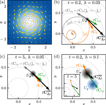
Figure 5: (a) Illustration of the steady-state density (color gradient) and current (arrows) of the two-dimensional rotational flow Eq. (2) with $\Omega=3$. Gray dotted lines in (a-d) are circles with radii $0.25,\,0.5,\,0.75,\,1$. (b-c) Single-point $\mathbf{x}=\mathbf{y}$ and (d) two-point time-accumulated correlation $t\mathbf{C}^{\mathbf{x}\mathbf{y}}_{\mathbf{J}\rho}$ at $t=0.2$ and $t=5$ (black arrow), with final-point $\mathbf{C}_{\rm fi}\equiv\hat{\mathcal{I}}^{t}_{\mathbf{x}\mathbf{y}}[\hat{\mathbf{j}}_{\mathbf{z}}P_{\mathbf{z}^{\prime}}(\mathbf{z},t^{\prime})-{\mathbf{j}}_{\rm s}(\mathbf{z})p_{\rm s}(\mathbf{z}^{\prime})]$ (orange) and initial-point $\mathbf{C}_{\rm in}$ (green) contribution, s. t. $\mathbf{C}^{\mathbf{x}\mathbf{y}}_{\mathbf{J}\rho}=\mathbf{C}_{\rm in}+\mathbf{C}_{\rm fi}$. $\mathbf{C}_{\rm fi}({\mathbf{j}}_{\rm s}\to-{\mathbf{j}}_{\rm s})$ (gray) is the current-reversed final-point contribution which agrees with the inverted initial-point contribution $-\mathbf{C}_{\rm in}$. Full lines in (b) are the mean trajectory $[\mu]\equiv\langle\mathbf{x}_{\tau\geq 0}\rangle_{\mathbf{x}_{0}=\mathbf{x}}$ (orange) and its current-reverse $[\mu^{{\mathbf{j}}_{\rm s}\to-{\mathbf{j}}_{\rm s}}]$ (gray). $U_{\mathbf{x},\mathbf{y}}$ (shaded circles) is a Gaussian at $\mathbf{x},\mathbf{y}$ with width $h$, see Eq. (3).

IV.6 Current (co)variance

Recall that the current (co)variance Eq. (29) involves scalar products of initial- and final-point increments ${\left\langle{\circ d\mathbf{x}_{t_{1}}\cdot\circ d\mathbf{x}_{t_{2}}}\right\rangle}^{\mathbf{x}_{t_{2}}=\mathbf{z}^{\prime}}_{\mathbf{x}_{t_{1}}=\mathbf{z}}$, which cannot be easily interpreted as scalar products of currents. They are not the scalar products of initial- and final-point currents, since ${\left\langle{\circ d\mathbf{x}_{t_{1}}\cdot\circ d\mathbf{x}_{t_{2}}}\right\rangle}^{\mathbf{x}_{t_{2}}=\mathbf{z}^{\prime}}_{\mathbf{x}_{t_{1}}=\mathbf{z}}\neq\left\langle{\circ d\mathbf{x}_{t_{1}}}\right\rangle^{\mathbf{x}_{t_{2}}=\mathbf{z}^{\prime}}_{\mathbf{x}_{t_{1}}=\mathbf{z}}\cdot\left\langle{\circ d\mathbf{x}_{t_{2}}}\right\rangle^{\mathbf{x}_{t_{2}}=\mathbf{z}^{\prime}}_{\mathbf{x}_{t_{1}}=\mathbf{z}}$. Rather they correspond to the scalar product of the initial- and final-point increment along the same trajectory and only then they become averaged over all trajectories from $\mathbf{z}$ to $\mathbf{z}^{\prime}$ (see also Fig. 2 in [58]). For $t_{1}<t_{2}$ these are computed equivalently to Eqs. (37)-(41) based on the Lemma (36) as

$$\left\langle{\circ d\mathbf{x}_{t_{1}}\cdot\circ d\mathbf{x}_{t_{2}}}\right\rangle^{\mathbf{x}_{t_{2}}=\mathbf{z}^{\prime}}_{\mathbf{x}_{t_{1}}=\mathbf{z}}={\hat{\mathbf{j}}}^{\ddagger}_{\mathbf{z}}\cdot\hat{\mathbf{j}}_{\mathbf{z}^{\prime}}P_{\mathbf{z}}(\mathbf{z}^{\prime},t^{\prime}).$$ (46)

However, according to the convention $\int_{t_{1}}^{t}dt_{2}\delta(t_{2}-t_{1})=1/2$ in Eq. (18), we also need to consider the case $t_{1}=t_{2}$, i.e. $t^{\prime}=0$, which did not contribute for $C_{\rho\rho}$ and $C_{\mathbf{J}\rho}$. In the case $t_{1}=t_{2}$ (recall the definition in Eq. (25))

$$\langle\circ d\mathbf{x}_{t_{1}} \cdot\circ d\mathbf{x}_{t_{2}}\rangle^{\mathbf{x}_{t_{2}}=\mathbf{z}^{\prime}}_{\mathbf{x}_{t_{1}}=\mathbf{z}}$$

$$\equiv \left\langle{\delta(\mathbf{x}_{t_{1}}-\mathbf{z})\circ d\mathbf{x}_{t_{1}}\cdot\delta(\mathbf{x}_{t_{2}}-\mathbf{z}^{\prime})\circ d\mathbf{x}_{t_{2}}}\right\rangle_{\rm s}$$

$$\overset{t_{1}=t_{2}}{=} \Big{\langle}\delta(\mathbf{x}_{t_{1}}-\mathbf{z})\sqrt{2\mathbf{D}(\mathbf{x}_{t_{1}})}d\mathbf{W}_{t_{1}}\cdot$$

$$\,\,\,\delta(\mathbf{x}_{t_{2}}-\mathbf{z}^{\prime})\sqrt{2\mathbf{D}(\mathbf{x}_{t_{2}})}d\mathbf{W}_{t_{2}}\Big{\rangle},$$ (47)

where we used that for $t_{1}=t_{2}$ the only term surviving is $d\mathbf{W}_{t_{1}}^{\,2}$ (and not $d\mathbf{W}_{t_{1}}dt_{1}$ and $dt_{1}^{2}$, which is why such terms only enter in current-current expressions but not in current-density or density-density correlations), as well as (by Itô’s isometry) $\int_{t_{1}}^{t}dt_{2}d\mathbf{W}^{j}_{t_{1}}\frac{d\mathbf{W}^{l}_{t_{2}}}{dt_{2}}=\delta_{jl}dt_{1}$. Using $P_{\mathbf{z}}(\mathbf{z}^{\prime},t^{\prime}=0)=\delta(\mathbf{z}-\mathbf{z}^{\prime})p_{\rm s}(\mathbf{z})$ we find for $t_{1}=t_{2}$

$$\left\langle{\circ d\mathbf{x}_{t_{1}}\cdot\circ d\mathbf{x}_{t_{2}}}\right\rangle^{\mathbf{x}_{t_{2}}=\mathbf{z}^{\prime}}_{\mathbf{x}_{t_{1}}=\mathbf{z}}$$

$$=P_{\mathbf{z}}(\mathbf{z}^{\prime},0)\sum_{i,j,l=1}^{d}[\sqrt{2\mathbf{D}(\mathbf{z})}]_{ij}[\sqrt{2\mathbf{D}(\mathbf{z}^{\prime})}]_{il}\delta(t_{1}-t_{2})\delta_{jl}dt_{1}$$

$$=p_{\rm s}(\mathbf{z})\delta(\mathbf{z}-\mathbf{z}^{\prime})\sum_{i=1}^{d}[2\mathbf{D}(\mathbf{z})]_{ii}\delta(t_{1}-t_{2})dt_{1}$$

$$=2{\rm Tr}[\mathbf{D}(\mathbf{z})]p_{\rm s}(\mathbf{z})\delta(\mathbf{z}-\mathbf{z}^{\prime})\delta(t_{1}-t_{2})dt_{1}.$$ (48)

Plugging this into Eq. (29), we obtain, using Eq. (46) and accounting for the $t^{\prime}=0$ contribution, the result for current covariances in the form of

$$C^{\mathbf{x}\mathbf{y}}_{\mathbf{J}\cdot\mathbf{J}}(t)=\frac{2}{t}\int d\mathbf{z}{\rm Tr}[\mathbf{D}(\mathbf{z})]U^{h}_{\mathbf{x}}(\mathbf{z})U^{h}_{\mathbf{y}}(\mathbf{z})p_{\rm s}(\mathbf{z})$$ (49)

$$+\hat{\mathcal{I}}_{\mathbf{x}\mathbf{y}}^{t,U}[{\hat{\mathbf{j}}}^{\ddagger}_{\mathbf{z}^{\prime}}\cdot\hat{\mathbf{j}}_{\mathbf{z}}P_{\mathbf{z}^{\prime}}(\mathbf{z},t^{\prime})+{\hat{\mathbf{j}}}^{\ddagger}_{\mathbf{z}}\cdot\hat{\mathbf{j}}_{\mathbf{z}^{\prime}}P_{\mathbf{z}}(\mathbf{z}^{\prime},t^{\prime})-2{\mathbf{j}}_{\rm s}(\mathbf{z})\cdot{\mathbf{j}}_{\rm s}(\mathbf{z}^{\prime})].$$

The second line is interpreted analogously to the current-density correlation in Eq. (45) with the only difference that the scalar product of current operators reflects scalar products of increments along individual trajectories. The first term, however, does not appear in $C^{\mathbf{x}\mathbf{y}}_{\mathbf{J}\rho}$ and $C^{\mathbf{x}\mathbf{y}}_{\rho\rho}$. As can be seen from the derivation in Eq. (48) this term originates from the purely diffusive (i.e. Brownian) term involving $d\mathbf{x}_{\tau}\cdot d\mathbf{x}_{\tau}=2{\rm Tr}\mathbf{D}(\mathbf{z})d\tau$ and only appears for $t_{1}=t_{2}$, i.e. $t^{\prime}=0$. Thus, this term cannot be interpreted in terms of trajectories from $\mathbf{z}$ to $\mathbf{z}^{\prime}$ or vice versa, but instead reflects that due to the nature of Brownian motion the square of instantaneous fluctuations $(d\mathbf{x}_{\tau})^{2}$ does not vanish but contributes on the order $d\tau$. Note that since here $\mathbf{z}=\mathbf{z}^{\prime}$ this term only contributes if $U^{h}_{\mathbf{x}}(\mathbf{z})$ and $U^{h}_{\mathbf{y}}(\mathbf{z}^{\prime})$ have non-zero overlap.

For $\mathbf{x}=\mathbf{y}$ the covariance becomes the current variance ${\rm var}_{\mathbf{J}}^{\mathbf{x}}(t)\equiv C^{\mathbf{x}\mathbf{y}}_{\mathbf{J}\cdot\mathbf{J}}(t)$ which plays a vital role in stochastic thermodynamics. As an application of the result in Eq. (49) we use the TUR-bound under concurrent variation of the coarse-graining scale $h$ to optimize the inference of a system’s dissipation via current fluctuations. Before we turn to this inference problem, we take a closer look at the limit of no coarse graining, i.e. $h\to 0$.

V The limit of no coarse graining

In this section we consider the variance ${\rm var}_{\rho}^{\mathbf{x}}(t)\equiv C^{\mathbf{x}\mathbf{x}}_{\rho\rho}(t),{\rm var}_{\mathbf{J}}^{\mathbf{x}}(t)\equiv C^{\mathbf{x}\mathbf{x}}_{\mathbf{J}\cdot\mathbf{J}}(t)$ and correlations $\mathbf{C}^{\mathbf{x}\mathbf{x}}_{\mathbf{J}\rho}(t)$ in Eqs. (23),(45),(49) with $\mathbf{x}=\mathbf{y}$ in the limit of no coarse graining, i.e. when $h\to 0$. In particular, we consider normalized window functions $\int d\mathbf{z}U^{h}_{\mathbf{x}}(\mathbf{z})=1$ such that in the limit of no coarse graining $U^{h\to 0}_{\mathbf{x}}(\mathbf{z})=\delta(\mathbf{x}-\mathbf{z})$ (see e.g. (3)). Thus, the density and current observables in Eq. (1) for $h=0$ correspond to the empirical density and current defined with a delta function

$$\overline{\rho_{\mathbf{x}}}(t) \equiv\frac{1}{t}\int_{0}^{t}\delta(\mathbf{x}-\mathbf{x}_{\tau})d\tau$$

$$\overline{\mathbf{J}_{\mathbf{x}}}(t) \equiv\frac{1}{t}\int_{\tau=0}^{\tau=t}\delta(\mathbf{x}-\mathbf{x}_{\tau})\circ d\mathbf{x}_{\tau},$$ (50)

which is the definition typically adopted in the literature [4, 60, 61, 62, 63, 7, 64, 65, 66, 67]. We show in Appendix A that in spatial dimensions $d\geq 2$ the variance and correlation functions diverge ${\rm var}_{\rho}^{\mathbf{x}}(t),{\rm var}_{\mathbf{J}}^{\mathbf{x}}(t),\mathbf{C}^{\mathbf{x}\mathbf{x}}_{\mathbf{J}\rho}(t)\to\infty$ as $h\to 0$. Note that the mean values Eqs. (15) and (17) of the observables Eq. (50) do not diverge but instead for $U^{h\to 0}_{\mathbf{x}}(\mathbf{z})=\delta(\mathbf{x}-\mathbf{z})$ directly simplify to $\left\langle{\overline{\rho_{\mathbf{x}}}(t)}\right\rangle_{\rm s}=p_{\rm s}(\mathbf{x})$ and $\left\langle{\overline{\mathbf{J}_{\mathbf{x}}}(t)}\right\rangle_{\rm s}={\mathbf{j}}_{\rm s}(\mathbf{x})$ (see also [4]).

Before we go into the specific results for the limit $h\to 0$, let us first discuss why divergent fluctuations of the functionals in Eq. (50), although overlooked so far, are in fact not surprising. The simplest argument is that second moments as e.g. $\left\langle{\overline{\rho_{\mathbf{x}}}(t)^{2}}\right\rangle_{\rm s}$ involve terms $\left\langle{\delta(\mathbf{x}-\mathbf{x}_{\tau})\delta(\mathbf{x}-\mathbf{x}_{\tau^{\prime}})}\right\rangle_{\rm s}$, which diverge for $\tau=\tau^{\prime}$ since a squared delta function appears. In contrast, the mean value $\left\langle{\overline{\rho_{\mathbf{x}}}(t)}\right\rangle_{\rm s}$ contains $\left\langle{\delta(\mathbf{x}-\mathbf{x}_{\tau})}\right\rangle_{\rm s}=p_{\rm s}(\mathbf{x})$ which is finite. Loosely speaking, the mean value involving $\left\langle{\delta(\mathbf{x}-\mathbf{x}_{\tau})}\right\rangle_{\rm s}$ is given by the probability to be at point $\mathbf{x}$, which is zero, multiplied by the height of the delta function at $\mathbf{x}$, which is infinite. Since the mean value is finite for $h\to 0$ this can be seen to yield “$0\times\infty=p_{\rm s}(\mathbf{x})$”, while the second moment contains a squared delta peak, such that the second moment loosely speaking diverges due to “$0\times\infty^{2}=p_{\rm s}(\mathbf{x})\times\infty=\infty$”. This argument illustrates that divergent fluctuations are not surprising but this argument is oversimplified since it does not take into account the time integration. In particular, to explain why the divergence only occurs in spatial dimensions $d\geq 2$, we have to note that due to the time integration the one-dimensional case is qualitatively different. Given some point $\mathbf{z}$ in $d$-dimensional space, the trajectory will hit $z\equiv\mathbf{z}$ with a finite probability in $d=1$ (i.e. with non-zero probability there is some $\tau\in[0,t]$ such that $x_{\tau}=z$; e.g. if $x_{0}<x_{t}$ all points in $[x_{0},x_{t}]$ are hit). This is qualitatively different for $d\geq 2$, since overdamped motion in $d\geq 2$ does not hit points, i.e. the probability to hit a given point $\mathbf{z}$ is zero, $\mathbbm{P}(\exists\tau\in(0,\infty)\colon\mathbf{x}_{\tau}=\mathbf{z})=0$ [59]. This property is not specific to overdamped motion, but is rather due to the fact that the set of points $(\mathbf{x}_{\tau})_{0\leq\tau\leq t}$ has Lebesgue measure zero for $d\geq 2$.

To further explain the divergence and its dependence on the dimensionality in a somewhat less oversimplified way (for the detailed derivation see Appendix A), we take a second look at the term $\left\langle{\delta(\mathbf{x}-\mathbf{x}_{\tau})\delta(\mathbf{x}-\mathbf{x}_{\tau^{\prime}})}\right\rangle_{\rm s}=G(\mathbf{x},\left\lvert\tau-\tau^{\prime}\right\rvert|\mathbf{x})p_{\rm s}(\mathbf{x})$ occurring in $\left\langle{\overline{\rho_{\mathbf{x}}}(t)^{2}}\right\rangle_{\rm s}$. Here, $G(\mathbf{x},t^{\prime}|\mathbf{x})$ trivially diverges if $t^{\prime}=0$. However, the relevant question is whether the return integral $\int_{0}^{t}G(\mathbf{x},t^{\prime}|\mathbf{x})dt^{\prime}$ diverges. Any divergence in the integral would come from $t^{\prime}\to 0$ where $G(\mathbf{x},t^{\prime}|\mathbf{x})$ diverges, i.e. from the limit of small time differences $\left\lvert\tau-\tau^{\prime}\right\rvert$. For $t^{\prime}\to 0$ the overdamped propagator $G(\mathbf{x},t^{\prime}|\mathbf{x})$ becomes Gaussian with variance $\propto Dt^{\prime}$ [78] (so for very small $t^{\prime}$ we have $G(\mathbf{x},t^{\prime}|\mathbf{x})\propto{t^{\prime}}^{-d/2}$ in $d$-dimensional space), and thus the return integral $\int_{0}^{t}G(\mathbf{x},t^{\prime}|\mathbf{x})dt^{\prime}$ diverges if and only if $\int_{0}^{t}{t^{\prime}}^{-d/2}dt^{\prime}$ diverges. Therefore the variance ${\rm var}_{\rho}^{\mathbf{x}}(t)$ diverges in spatial dimensions $d\geq 2$.

Apart from the two arguments above providing mathematical intuition about the divergence, there is also a physical intuition that suggests divergent fluctuations. Recall that for finite $h>0$, the observables $\overline{\rho^{U}_{\mathbf{x}}}$ and $\overline{\mathbf{J}^{U}_{\mathbf{x}}}$ in Eq. (1) by definition measure the time and displacement that the trajectory $(x_{\tau})_{0\leq\tau\leq t}$ accumulates in the region $U^{h}_{\mathbf{x}}$ of scale $h$ around $\mathbf{x}$. Now as $h\to 0$, only visitations of precisely the point $\mathbf{x}$ contribute. Two very similar (but not equal) trajectories may now give very different values for $\overline{\rho^{U}_{\mathbf{x}}}$ and $\overline{\mathbf{J}^{U}_{\mathbf{x}}}$, depending whether the point $\mathbf{x}$ is hit or even slightly missed (e.g. by a distance $h$). Therefore, fluctuations among different trajectories of these functionals diverge as $h\to 0$. This reasoning is not restricted to overdamped stochastic motion, and indeed seems to hold for more general dynamics, see outlook in Sec. X.

This simple illustration also explains why fluctuations do not diverge in one-dimensional space. There, points are hit, meaning that e.g. a trajectory starting at $0$ and ending at $1$ always hits all points in between at some intermediate time, which is why the density and current observables have qualitatively lower fluctuations compared to higher dimensions. The reason that the divergence for $d\geq 2$ was overlooked so far is probably due to the fact that most explicit examples were analyzed in one-dimensional space only.

Explicitly, in the limit $h\to 0$ the expressions Eqs. (23), (45),(49) with $\mathbf{x}=\mathbf{y}$ for any time $t$ take the form

$${\rm var}^{\mathbf{x}}_{\rho}(t)\!\! \overset{h\to 0}{\simeq}\frac{K}{\tilde{D}_{\mathbf{x}}t}p_{\rm s}(\mathbf{x})\begin{cases}\frac{h^{2-d}}{d-2}&\text{for}\>d>2\\ -\ln{h}&\text{for}\>d=2\end{cases}$$

$$\mathbf{C}^{\mathbf{x}\mathbf{x}}_{\mathbf{J}\rho}(t)\!\! \overset{h\to 0}{\simeq}{\mathbf{j}}_{\rm s}(\mathbf{x}){\rm var}^{\mathbf{x}}_{\rho}(t)/2p_{\rm s}(\mathbf{x})$$ (51)

$$\text{var}^{\mathbf{x}}_{\mathbf{J}}(t)\!\! \overset{h\to 0}{=}\!\!K^{\prime}\frac{2\tilde{D}^{\prime}_{\mathbf{x}}}{t}p_{\rm s}(\mathbf{x})(d-1)h^{-d}\!+\mathcal{O}(t^{-1})\mathcal{O}(h^{1-d}),$$

where $\simeq$ denotes asymptotic equality, $\tilde{D}_{\mathbf{x}},\tilde{D}^{\prime}_{\mathbf{x}}$ are constants bounded by the smallest and largest eigenvalues of $\mathbf{D}(\mathbf{x})$, and $K,K^{\prime}$ are constants depending on the specific normalized window $U^{h}_{\mathbf{z}}$ (see Appendix A). Note that the dominant term in $\text{var}^{\mathbf{x}}_{\mathbf{J}}(t)$ vanishes for $d=1$ such that all three expressions only diverge for $d\geq 2$. Some details on the case $d=1$ are shown in Appendix A.4.

Thus, the empirical density and current as defined in Eq. (50) have divergent fluctuations. Note that an infinite variance contradicts Gaussian statistics on all time scales. This divergence, moreover, leads us to question whether Eq. (50) is even well-defined, i.e. whether these observables are mathematically well-defined random variables, and whether the result in the limit $h\to 0$ is unaffected by the specific choice of the $U^{h}_{\mathbf{x}}$ as long as $U^{h\to 0}_{\mathbf{x}}(\mathbf{z})=\delta(\mathbf{x}-\mathbf{z})$.

VI Application to inference of dissipation

We now apply the results for the current variance ${\rm var}_{\mathbf{J}}^{\mathbf{x}}(t)\equiv C^{\mathbf{x}\mathbf{x}}_{\mathbf{J}\cdot\mathbf{J}}(t)$ in Eq. (49) for $\mathbf{x}=\mathbf{y}$. For an individual component, e.g. $J_{y}\equiv[\overline{\mathbf{J}^{U}_{\mathbf{x}}}]_{y}$, of the vector $\overline{\mathbf{J}^{U}_{\mathbf{x}}}$ the equivalent result reads

$${\rm var}^{\mathbf{x}}_{J_{y}}(t)\!=\!\frac{2}{t}\!\int\!\!d\mathbf{z}[\mathbf{D}(\mathbf{z})]_{yy}U^{h}_{\mathbf{x}}(\mathbf{z})U^{h}_{\mathbf{x}}(\mathbf{z})p_{\rm s}(\mathbf{z})+\hat{\mathcal{I}}_{\mathbf{x}\mathbf{y}}^{t,U}[({\hat{\mathbf{j}}}^{\ddagger}_{\mathbf{z}^{\prime}})_{y}\times$$

$$(\hat{\mathbf{j}}_{\mathbf{z}})_{y}P_{\mathbf{z}^{\prime}}(\mathbf{z},t^{\prime})+({\hat{\mathbf{j}}}^{\ddagger}_{\mathbf{z}})_{y}(\hat{\mathbf{j}}_{\mathbf{z}^{\prime}})_{y}P_{\mathbf{z}}(\mathbf{z}^{\prime},t^{\prime})-2[{\mathbf{j}}_{\rm s}(\mathbf{z})]_{y}[{\mathbf{j}}_{\rm s}(\mathbf{z}^{\prime})]_{y}].$$ (52)

With the dissipation rate $\dot{\Sigma}$ in Eq. (10), current observables such as $J_{y}\equiv[\overline{\mathbf{J}^{U}_{\mathbf{x}}}]_{y}$ satisfy the TUR [34, 15] (in the form relevant below first proven in [15])

$$\frac{{\rm var}^{\mathbf{x}}_{J_{y}}(t)}{\left\langle{J_{y}}\right\rangle_{\rm s}^{2}}\geq\frac{2}{t\dot{\Sigma}}.$$ (53)

This bound is of particular interest since it allows to infer a lower bound on a system’s dissipation from measurements of the local mean current and current fluctuations [17, 82, 83, 84, 53]. Note that Eq. (53) implicitly assumes “perfect” statistics, i.e. $\left\langle{J_{y}}\right\rangle_{\rm s}$ and ${\rm var}^{\mathbf{x}}_{J_{y}}(t)$ are the exact mean and variance for the process under consideration (not limited by sampling constraints on a finite number of realizations).

We now investigate the influence of the coarse graining on the sharpness of the bound (53). One might naively expect that coarse graining annihilates information. However, as shown in [58] the current fluctuations diverge in spatial dimensions $d\geq 2$ in the limit $h\to 0$ (of no coarse graining), whereas the mean converges to a constant (note that $\dot{\Sigma}$ does not at all depend on $U^{h}_{\mathbf{x}}$). The exact asymptotics for $h\to 0$ in [58] demonstrate that the bound (53) becomes entirely independent of the process (i.e. it only depends on $p_{\rm s}$ but contains no information about the non-equilibrium part of the dynamics). Therefore, the left hand side of the inequality (53) tends to $\infty$ as $h\to 0$, rendering the TUR without spatial coarse graining unable to infer dissipation beyond the statement $\dot{\Sigma}\geq 0$ for $h=0$.

However, the naive intuition is correct in the limit of “ignorant” coarse graining $h\to\infty$, where $U^{h}_{\mathbf{x}}$ becomes asymptotically constant in a sufficiently large hypervolume centered at $\mathbf{x}$ (i.e. in a hypervolume ${\rm A}$ where $\int_{\rm A}p_{\rm s}(\mathbf{x})d\mathbf{x}\approx 1$). The integration over a constant $U^{h}_{\mathbf{x}}=c$ yields $\left\langle{\overline{\mathbf{J}^{U}_{\mathbf{x}}}(t)}\right\rangle_{\rm s}=c\int d\mathbf{z}{\mathbf{j}}_{\rm s}(\mathbf{z})=\mathbf{0}$ for the mean Eq. (17). The vanishing $\left\langle{\overline{\mathbf{J}^{U}_{\mathbf{x}}}(t)}\right\rangle_{\rm s}$ may be seen in two ways. First, since $\nabla_{\mathbf{z}}\cdot{\mathbf{j}}_{\rm s}(\mathbf{z})=0$, curl ${\mathbf{j}}_{\rm s}(\mathbf{z})=\nabla_{\mathbf{z}}\times\mathbf{f}(\mathbf{z})$ and by Stokes theorem $\int_{\rm A}d^{2}z\nabla_{\mathbf{z}}\times\mathbf{f}(\mathbf{z})=\int_{\partial\rm A}\mathbf{f}\cdot d\mathbf{l}$ which vanishes since at the boundary $\partial{\rm A}$ at $\infty$ we have $p_{\rm s}\to 0$, thus ${\mathbf{j}}_{\rm s}\to 0$ and therefore the vector potential $\mathbf{f}\to\mathbf{0}$. Second, for $U^{h}_{\mathbf{x}}=c$ we have $\overline{\mathbf{J}^{U}_{\mathbf{x}}}(t)=\frac{c}{t}(\mathbf{x}_{t}-\mathbf{x}_{0})$ (and we assume $\mathbf{x}_{0}$ to be sampled from $p_{\rm s}(\mathbf{x})$). Then $\mathbf{x}_{0}$ and $\mathbf{x}_{t}$ are both distributed according to $p_{\rm s}$, thus $\left\langle{\mathbf{x}_{t}}\right\rangle_{\rm s}=\left\langle{\mathbf{x}_{0}}\right\rangle_{\rm s}$ and $t\left\langle{\overline{\mathbf{J}^{U}_{\mathbf{x}}}(t)}\right\rangle_{\rm s}/c=\left\langle{\mathbf{x}_{t}}\right\rangle_{\rm s}-\left\langle{\mathbf{x}_{0}}\right\rangle_{\rm s}=0$. Conversely, the variance remains strictly positive. Therefore, also for $h\to\infty$ the left hand side of the inequality (53) diverges, rendering the TUR with an “ignorant” coarse graining incapable of inferring dissipation (again only gives $\dot{\Sigma}\geq 0$ as for $h=0$).

These two arguments, i.e. the necessity of coarse graining [58] and the failure of an “ignorant” coarse graining, imply that an intermediate coarse graining exists that is optimal for inferring dissipation via the TUR (53).

We first demonstrate this finding using a two-dimensional rotational flow (2) with Gaussian coarse graining window Eq. (3). We evaluate the left hand side of Eq. (53) for varying $h$ and $\mathbf{x}$ and compare it to the constant right hand side of Eq. (53). Particularly for $\mathbf{D}(\mathbf{z})=D\mathbf{1}$, we have $p_{\rm s}(\mathbf{z})=r/(2\pi D)\exp(-r\mathbf{z}^{2}/(2D))$ and ${\mathbf{j}}_{\rm s}(\mathbf{z})=\Omega p_{\rm s}(\mathbf{z})(z_{2},\,-z_{1})^{T}$ and the dissipation rate Eq. (10) is given by

$$\dot{\Sigma} =\int d\mathbf{z}\frac{{\mathbf{j}}_{\rm s}^{T}(\mathbf{z})}{p_{\rm s}(\mathbf{z})}\mathbf{D}^{-1}(\mathbf{z})\frac{{\mathbf{j}}_{\rm s}(\mathbf{z})}{p_{\rm s}(\mathbf{z})}p_{\rm s}(\mathbf{z})=\frac{\Omega^{2}}{D}\int d\mathbf{z}\,\mathbf{z}^{2}p_{\rm s}(\mathbf{z})$$

$$=\frac{\Omega^{2}}{D}\left\langle{\mathbf{x}_{0}^{2}}\right\rangle_{\rm s}=\frac{\Omega^{2}}{D}\left\langle{x_{1}^{2}+x_{2}^{2}}\right\rangle_{\rm s}=\frac{\Omega^{2}}{D}2\frac{D}{r}=\frac{2\Omega^{2}}{r}.$$ (54)

Thus the TUR in Eq. (53) for the rotational flow becomes

$$\frac{{\rm var}^{\mathbf{x}}_{J_{y}}(t)}{\left\langle{J_{y}}\right\rangle_{\rm s}^{2}}\geq\frac{r}{t\Omega^{2}}.$$ (55)

The results shown in Fig. 6a-d demonstrate, as argued above, that relative fluctuations diverge as $h\to 0,\infty$. For this example, the relative error as a function of $h$ has a unique minimum (slightly depending on $\mathbf{x}$, and possibly on other parameters such as $t$). This means that (restricted to $U^{h}_{\mathbf{x}}$ being a Gaussian around $\mathbf{x}$) there is a coarse graining scale $h$ that is optimal for inferring a lower bound on the dissipation, that may also provide some intuition about the formal optimization carried out in [84]. This result demonstrates that coarse graining trajectory data a posteriori can improve the inference of thermodynamical information, which is a strong motivation for considering coarse graining.

In particular, note that this method is readily applicable, i.e. one does not need to know the underlying process (as long as the dynamics is overdamped). As was done in Fig 6e-h one simply integrates the trajectories to obtain the coarse grained current as defined in Eq. (1). Then, the mean and variance are readily obtained from the fluctuations along an ensemble of individual trajectories, and for each value of $\mathbf{x}$ and $h$ one determines a lower bound on the dissipation via Eq. (53). Finally, one takes the best of those bounds. We here only consider Gaussian $U^{h}_{\mathbf{x}}$ for the coarse graining, but due to the flexibility of the theory one could even choose window functions that do not have to relate to the notion of coarse graining. Notably, a Gaussian window function is in this case better than e.g. a rectangular indicator function (which one usually uses for binning data) due to an improved smoothing effect. Moreover, one further expects a reduced error due to discrete-time effects.

Note that compared to many of the similar existing methods [56, 17, 54], we neither advise to rasterize the continuous dynamics to parameterize (i.e. “count”) currents nor to approximate the dynamics by a Markov-jump process. Our method is therefore not only correct (note that a Markov-jump assumption is only accurate in the presence of a time-scale separation ensuring a local equilibration, e.g. as a results of high barriers separating energy minima) but also has the great advantage of not having to parameterize rates at all. Instead one simply integrates trajectories according to Eq. (1).

A generalization to windows that are not centered at individual points as well as the use of correlations in Eq. (45) entering the recent so-called CTUR inequality [56] will be considered in forthcoming publications.

To underscore the applicability of the above inference strategy, we apply it to a more complicated system, for which a Markov jump process description would be difficult due to the presence of low and flat barriers and extended states. The results are shown Fig. 6e-h. The example is constructed by considering the two-dimensional potential

$$\phi(x,y)= 0.75(x^{2}-1)^{2}+$$

$$(y^{2}-1.5)^{2}((x+0.5y-0.5)^{2}+0.5)+c$$ (56)

where $c$ is a constant such that $p_{\rm s}(\mathbf{z})=\exp[-\phi(\mathbf{z})]$ is normalized. We consider isotropic additive noise $\mathbf{D}(\mathbf{z})=D\mathbf{1}$ and construct the Itô/Langevin equation for the process as

$$d\mathbf{x}_{\tau}=-D\{\nabla\phi\}(\mathbf{x}_{\tau})d\tau+\mathbf{F}^{\rm irrev}(\mathbf{x}_{\tau})+\sqrt{2D}d\mathbf{W}_{\tau},$$ (57)

where

$$\mathbf{F}^{\rm irrev}(\mathbf{z})=\frac{{\mathbf{j}}_{\rm s}(\mathbf{z})}{p_{\rm s}(\mathbf{z})}\equiv-D\Omega\begin{bmatrix}0&-1\\ 1&0\end{bmatrix}\cdot\{\nabla\phi\}(\mathbf{z}),$$ (58)

is an irreversible drift that is by construction orthogonal to $\nabla\phi$ and thus does not alter the steady-state (i.e. same $p_{\rm s}=\exp[-\phi]$ for equilibrium ($\Omega=0$) or any other $\Omega$). With Eq. (58) the dissipation in Eq. (10) for this process reads

$$\dot{\Sigma}=D\Omega^{2}\int{\rm d}^{2}\mathbf{x}\{\nabla\phi\}(\mathbf{x})^{T}\begin{bmatrix}0&-1\\ 1&0\end{bmatrix}^{T}\begin{bmatrix}0&-1\\ 1&0\end{bmatrix}\cdot$$ (59)

$$\{\nabla\phi\}(\mathbf{x})p_{s}(\mathbf{x})=D\Omega^{2}\int{\rm d}^{2}\mathbf{x}\{\nabla\phi\}^{2}(\mathbf{x})\exp\left[-\phi(\mathbf{x})\right],$$

which is solved numerically and gives $\dot{\Sigma}=19.65D\Omega^{2}$. We see in Fig. 6h that some intermediate coarse graining $h$ is still optimal, but the optimal scale $h$ now depends more intricately on $\mathbf{x}$ and the curves are not convex in $h$ anymore.

Overall we see that the approach is robust and easily applicable, and does not require to determine and parameterize any rates. Moreover, due to the implications of the theory to the limits $h\to 0,\infty$ we can assert that some intermediate coarse graining will generally be optimal.

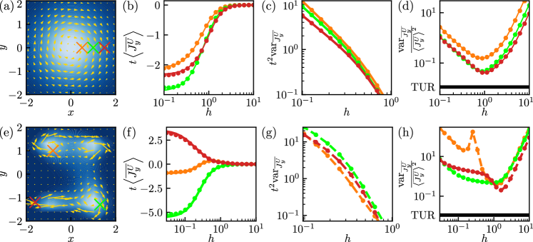
Figure 6: (a) Steady-state density (blue color gradient) and current (yellow arrows) for the rotational flow Eq. (2) with $\Omega=3$. Points around which the currents are evaluated in (b-d) are denoted by colored crosses. (b) Simulated values (circles) of the mean $y$-component of the time-integrated current from $2,000$ trajectories of length $t=10$ with time-step $dt=0.001$ (using the stochastic Euler algorithm) starting from steady-state initial conditions using a Gaussian window function Eq. (3) with different coarse-graining scales $h$. Analytical results Eq. (17) are shown with lines. (c) As in (b) but for variances. Simulations (circles) are shown alongside analytical results (lines; the results are analytic up to one time-integration, see Eq. (52)) for the variance of currents. (d) The relative error (ratio of variance and mean-squared) as a function of $h$ features a minimum at an intermediate $h$. At this minimum, the current fluctuations give the best lower bound on the dissipation via the TUR (53) at the value $2/(t\dot{\Sigma})=2/(10\times 18)=0.011$ (black line). (e) As in (a) but for the more complicated process in Eq. (57) with $D=1$ and we choose $\Omega=0.957$ to have the same dissipation as in (d); here the dissipation is obtained by means of a numerical integration. (f) As in (b) but for the process in (e) the “analytical” mean (17) had to be evaluated by means of a numerical integration. (g) As in (c) but simulated values are shown by circles and dashed line (but without a comparison to results of numerical integration since these require the knowledge of the propagator). (h) As in (d) but for the process in (e). The relative error may display several local minima. Some intermediate $h$ still allows for an optimal inference of the dissipation via the TUR (black line). Note that the relative error diverges (orange line) where the mean crosses zero (orange line in (b)).

VII Simplifications and symmetries

In this section we list the symmetries obeyed by the results in Eqs. (15),(17),(23),(45),(49) (with integral operator (22)). Note that the limit $h\to 0$ was carried out in Sec. V and the limit $h\to\infty$ gives $U^{h}_{\mathbf{x}}=c$ as noted before which greatly simplifies the further analysis. The limits $t\to 0$ and $t\to\infty$ will be addressed in Section IX (see also Supplemental Material in [58]).

First consider dynamics obeying detailed balance, i.e. ${\mathbf{j}}_{\rm s}=\mathbf{0}$. We then have ${\hat{\mathbf{j}}}^{\ddagger}_{\mathbf{z}}=-\hat{\mathbf{j}}_{\mathbf{z}}=-\hat{\mathbf{j}}^{g}(\mathbf{z})$ and the dual-reversal symmetry in Eq. (11), simplifies to the detailed balance statement $G(\mathbf{y},t|\mathbf{x})p_{\rm s}(\mathbf{x})=G(\mathbf{x},t|\mathbf{y})p_{\rm s}(\mathbf{y})$ or $P_{\mathbf{z}}(\mathbf{z}^{\prime},t)=P_{\mathbf{z}^{\prime}}(\mathbf{z},t)$. From this we obtain the following simplifications for ${\mathbf{j}}_{\rm s}=\mathbf{0}$:

$$\left\langle{\overline{\mathbf{J}^{U}_{\mathbf{x}}}(t)}\right\rangle_{\rm s}=\mathbf{0},\quad\mathbf{C}^{\mathbf{x}\mathbf{y}}_{\mathbf{J}\rho}(t)=\mathbf{0}$$

$$C^{\mathbf{x}\mathbf{y}}_{\rho\rho}(t)=2\hat{\mathcal{I}}^{t,U}_{\mathbf{x}\mathbf{y}}\left[P_{\mathbf{z}}(\mathbf{z}^{\prime},t^{\prime})-p_{\rm s}(\mathbf{z})p_{\rm s}(\mathbf{z}^{\prime})\right],$$

$$C^{\mathbf{x}\mathbf{y}}_{\mathbf{J}\cdot\mathbf{J}}(t)=\frac{2}{t}\int d\mathbf{z}{\rm Tr}[\mathbf{D}(\mathbf{z})]U^{h}_{\mathbf{x}}(\mathbf{z})U^{h}_{\mathbf{y}}(\mathbf{z})p_{\rm s}(\mathbf{z})$$

$$-2\hat{\mathcal{I}}_{\mathbf{x}\mathbf{y}}^{t,U}[\hat{\mathbf{j}}^{g}(\mathbf{z})\cdot\hat{\mathbf{j}}^{g}(\mathbf{z}^{\prime})P_{\mathbf{z}}(\mathbf{z}^{\prime},t^{\prime})+{\mathbf{j}}_{\rm s}(\mathbf{z})\cdot{\mathbf{j}}_{\rm s}(\mathbf{z}^{\prime})].$$ (60)

For the remainder of this section we consider ${\mathbf{j}}_{\rm s}\neq\mathbf{0}$. Note that by definition the interchange $\mathbf{x}\leftrightarrow\mathbf{y}$ leaves $C^{\mathbf{x}\mathbf{y}}_{\rho\rho}(t)$ and $C^{\mathbf{x}\mathbf{y}}_{\mathbf{J}\cdot\mathbf{J}}(t)$ invariant, but not $C^{\mathbf{x}\mathbf{y}}_{\mathbf{J}\rho}(t)$ since it considers currents at $\mathbf{x}$ and densities at $\mathbf{y}$.

For single-point correlations and variances $\mathbf{x}=\mathbf{y}$ (more precisely $U^{h}_{\mathbf{x}}=U^{h}_{\mathbf{y}}$) the integrations over $\mathbf{z}$ and $\mathbf{z}^{\prime}$ are equivalent and thus the results simplify to

$$C^{\mathbf{x}\mathbf{x}}_{\rho\rho}(t)=2\hat{\mathcal{I}}^{t,U}_{\mathbf{x}\mathbf{x}}\left[P_{\mathbf{z}}(\mathbf{z}^{\prime},t^{\prime})-p_{\rm s}(\mathbf{z})p_{\rm s}(\mathbf{z}^{\prime})\right]$$

$$\mathbf{C}^{\mathbf{x}\mathbf{x}}_{\mathbf{J}\rho}(t)=\hat{\mathcal{I}}_{\mathbf{x}\mathbf{x}}^{t,U}[(\hat{\mathbf{j}}_{\mathbf{z}^{\prime}}+{\hat{\mathbf{j}}}^{\ddagger}_{\mathbf{z}})P_{\mathbf{z}}(\mathbf{z}^{\prime},t^{\prime})-2{\mathbf{j}}_{\rm s}(\mathbf{z})p_{\rm s}(\mathbf{z}^{\prime})]$$

$$C^{\mathbf{x}\mathbf{x}}_{\mathbf{J}\cdot\mathbf{J}}(t)=\frac{2}{t}\int d\mathbf{z}{\rm Tr}[\mathbf{D}(\mathbf{z})][U^{h}_{\mathbf{x}}]^{2}(\mathbf{z})p_{\rm s}(\mathbf{z})$$

$$+2\hat{\mathcal{I}}_{\mathbf{x}\mathbf{x}}^{t,U}[{\hat{\mathbf{j}}}^{\ddagger}_{\mathbf{z}}\cdot\hat{\mathbf{j}}_{\mathbf{z}^{\prime}}P_{\mathbf{z}}(\mathbf{z}^{\prime},t^{\prime})-{\mathbf{j}}_{\rm s}(\mathbf{z})\cdot{\mathbf{j}}_{\rm s}(\mathbf{z}^{\prime})].$$ (61)

Now we again allow $\mathbf{x}\neq\mathbf{y}$ and consider the process and the ${\mathbf{j}}_{\rm s}\leftrightarrow-{\mathbf{j}}_{\rm s}$ inverted process. Then, from Eq. (11) and $[{\hat{\mathbf{j}}}^{\ddagger}_{\mathbf{z}^{\prime}}\cdot\hat{\mathbf{j}}_{\mathbf{z}}]^{-{\mathbf{j}}_{\rm s}}=-\hat{\mathbf{j}}_{\mathbf{z}^{\prime}}\cdot[-{\hat{\mathbf{j}}}^{\ddagger}_{\mathbf{z}}]=\hat{\mathbf{j}}_{\mathbf{z}^{\prime}}\cdot{\hat{\mathbf{j}}}^{\ddagger}_{\mathbf{z}}={\hat{\mathbf{j}}}^{\ddagger}_{\mathbf{z}}\cdot\hat{\mathbf{j}}_{\mathbf{z}^{\prime}}$, we get $[{\hat{\mathbf{j}}}^{\ddagger}_{\mathbf{z}^{\prime}}\cdot\hat{\mathbf{j}}_{\mathbf{z}}P_{\mathbf{z}^{\prime}}(\mathbf{z},t^{\prime})]^{-{\mathbf{j}}_{\rm s}}={\hat{\mathbf{j}}}^{\ddagger}_{\mathbf{z}}\cdot\hat{\mathbf{j}}_{\mathbf{z}^{\prime}}P_{\mathbf{z}}(\mathbf{z}^{\prime},t^{\prime})$ and thus obtain

$$\left\langle{\overline{\rho^{U}_{\mathbf{x}}}(t)}\right\rangle_{\rm s} =\left\langle{\overline{\rho^{U}_{\mathbf{x}}}(t)}\right\rangle_{\rm s}^{-{\mathbf{j}}_{\rm s}}$$

$$\left\langle{\overline{\mathbf{J}^{U}_{\mathbf{x}}}(t)}\right\rangle_{\rm s} =-\left\langle{\overline{\mathbf{J}^{U}_{\mathbf{x}}}(t)}\right\rangle_{\rm s}^{-{\mathbf{j}}_{\rm s}}$$

$$C^{\mathbf{x}\mathbf{y}}_{\rho\rho}(t) =[C^{\mathbf{x}\mathbf{y}}_{\rho\rho}(t)]^{-{\mathbf{j}}_{\rm s}}$$

$$\mathbf{C}^{\mathbf{x}\mathbf{y}}_{\mathbf{J}\rho}(t) =-[\mathbf{C}^{\mathbf{x}\mathbf{y}}_{\mathbf{J}\rho}(t)]^{-{\mathbf{j}}_{\rm s}}$$

$$C^{\mathbf{x}\mathbf{y}}_{\mathbf{J}\cdot\mathbf{J}}(t) =[C^{\mathbf{x}\mathbf{y}}_{\mathbf{J}\cdot\mathbf{J}}(t)]^{-{\mathbf{j}}_{\rm s}}.$$ (62)

In addition to the symmetries of the first and second cumulants, a stronger path-wise version of the dual-reversal symmetry in Eq. (11) (or time-reversal symmetry at equilibrium) dictates symmetries of the full distributions of the functionals of steady-state trajectories under the reversal ${\mathbf{j}}_{\rm s}\leftrightarrow-{\mathbf{j}}_{\rm s}$. Notably, at equilibrium (${\mathbf{j}}_{\rm s}=\mathbf{0}$) these simplify to symmetries of the process (which is a much stronger result since we do not have to compare to another (artificial) process with an inverted ${\mathbf{j}}_{\rm s}$).

To motivate this stronger symmetry, note that for steady-state initial conditions for any finite set of times $t_{1}<t_{2}<\dots<t_{n}$ we have that the joint density $P_{n}(\dots)$ for positions $z_{i}$ at equally spaced times $t_{i}=i\times\Delta t$ for $i=0,1,\dots,n$ is given by (since we have a Markov process by definition, i.e. Eq. (4) has no memory)

$$P_{n}(z_{0},t_{0};z_{1},t_{1};\dots;z_{n},t_{n})$$

$$=p_{\rm s}(\mathbf{x}_{0})G(\mathbf{x}_{1},\Delta t|\mathbf{x}_{0})\cdots G(\mathbf{x}_{n},\Delta t|\mathbf{x}_{n-1}).$$ (63)

By applying the dual-reversal symmetry Eq. (11) $n-1$ times, we obtain

$$P_{n}(z_{0},t_{0};z_{1},t_{1};\dots;z_{n},t_{n})$$

$$=G^{-{\mathbf{j}}_{\rm s}}(\mathbf{x}_{0},\Delta t|\mathbf{x}_{1})\cdots G^{-{\mathbf{j}}_{\rm s}}(\mathbf{x}_{n-1},\Delta t|\mathbf{x}_{n})p_{\rm s}(\mathbf{x}_{n})$$

$$=P^{-{\mathbf{j}}_{\rm s}}_{n}(z_{n},0;z_{n-1},\Delta t;\dots;z_{0},n\Delta t)$$

$$=P^{-{\mathbf{j}}_{\rm s}}_{n}(z_{n},t_{0};z_{n-1},t_{1};\dots;z_{0},t_{n}).$$ (64)

The $n+1$ points $(z_{1},\dots,z_{n})$ represent a discrete-time path for which Eq. (64) implies the path-wise discrete-time dual-reversal symmetry (denote $t=t_{n}=n\Delta t$)

$$P_{n}(z_{0},t_{0};z_{1},t_{1};\dots;z_{n},t_{n})$$

$$=P^{-{\mathbf{j}}_{\rm s}}_{n}(z_{n},t-t_{n};z_{n-1},t-t_{n-1};\dots;z_{0},t-t_{0}),$$ (65)

i.e. the probability of forward paths $(\mathbf{x}_{t_{i}})_{i=0,1,\dots,n}$ agrees with the probability of backwards paths of the process with inverted steady-state current ${\mathbf{j}}_{\rm s}\to-{\mathbf{j}}_{\rm s}$, i.e.

$$\mathbb{P}\left[(\mathbf{x}_{t_{i}})_{i=0,1,\dots,n}\right]=\mathbb{P}^{-{\mathbf{j}}_{\rm s}}\left[(\mathbf{x}_{t-t_{i}})_{i=0,1,\dots,n}\right].$$ (66)

Note that at equilibrium, ${\mathbf{j}}_{\rm s}=\mathbf{0}$, this is nothing but the detailed balance for discrete-time paths.

Assuming that one can take a continuum limit $\Delta t\to 0$ (and that a resulting path measure exits) one could conclude that continuous time paths fulfill the symmetry (see also [55])

$$\mathbb{P}\left[(\mathbf{x}_{\tau})_{0\leq\tau\leq t}\right]=\mathbb{P}^{-{\mathbf{j}}_{\rm s}}\left[(\mathbf{x}_{t-\tau})_{0\leq\tau\leq t}\right].$$ (67)

Based on this strong symmetry, and noting that densities are symmetric while currents are antisymmetric under time reversal, i.e.

$$\overline{\rho^{U}_{\mathbf{x}}}\left[(x_{\tau})_{0\leq\tau\leq t}\right] =\overline{\rho^{U}_{\mathbf{x}}}\left[(x_{t-\tau})_{0\leq\tau\leq t}\right]$$

$$\overline{\mathbf{J}^{U}_{\mathbf{x}}}\left[(x_{\tau})_{0\leq\tau\leq t}\right] =-\overline{\mathbf{J}^{U}_{\mathbf{x}}}\left[(x_{t-\tau})_{0\leq\tau\leq t}\right],$$ (68)

we obtain the following symmetries

$$\mathbb{P}\left[\overline{\rho^{U}_{\mathbf{x}}}(t)=u\right] =\mathbb{P}^{-{\mathbf{j}}_{\rm s}}\left[\overline{\rho^{U}_{\mathbf{x}}}(t)=u\right]$$

$$\mathbb{P}\left[\overline{\mathbf{J}^{U}_{\mathbf{x}}}(t)=\mathbf{u}\right] =\mathbb{P}^{-{\mathbf{j}}_{\rm s}}\left[\overline{\mathbf{J}^{U}_{\mathbf{x}}}(t)=-\mathbf{u}\right].$$ (69)

Eq. (69) implies symmetries for mean values and variances ($\mathbf{x}=\mathbf{y}$) listed in Eq. (62) since it implies that all moments of $\overline{\rho^{U}_{\mathbf{x}}}(t)$ agree and that the $n$-th moment of a current component $i$ fulfills $\left\langle{{[\overline{\mathbf{J}^{U}_{\mathbf{x}}}(t)]_{i}}^{\!n}}\right\rangle_{\rm s}=\left\langle{{[-\overline{\mathbf{J}^{U}_{\mathbf{x}}}(t)]_{i}}^{\!n}}\right\rangle_{\rm s}^{-{\mathbf{j}}_{\rm s}}=(-1)^{n}\left\langle{{[\overline{\mathbf{J}^{U}_{\mathbf{x}}}(t)]_{i}}^{\!n}}\right\rangle_{\rm s}^{-{\mathbf{j}}_{\rm s}}$.

Note that Eq. (69) implies that the statistics of $\rho(t)$ (incl. all moments) in general depends on ${\mathbf{j}}_{\rm s}$ but is invariant under the inversion ${\mathbf{j}}_{\rm s}\leftrightarrow-{\mathbf{j}}_{\rm s}$. Moreover, current fluctuations at equilibrium (${\mathbf{j}}_{\rm s}=\mathbf{0}$, hence $\mathbb{P}_{\rm EQ}\equiv\mathbb{P}=\mathbb{P}^{-{\mathbf{j}}_{\rm s}}$) are symmetric around the mean $\left\langle{\overline{\mathbf{J}^{U}_{\mathbf{x}}}}\right\rangle_{\rm s}=\mathbf{0}$, i.e.

$$\mathbb{P}_{\rm EQ}\left[\overline{\mathbf{J}^{U}_{\mathbf{x}}}(t)=\mathbf{u}\right] =\mathbb{P}_{\rm EQ}\left[\overline{\mathbf{J}^{U}_{\mathbf{x}}}(t)=-\mathbf{u}\right].$$ (70)

The symmetries for correlations in Eq. (62), possibly with $\mathbf{x}\neq\mathbf{y}$, may be seen as implications of the more general symmetries

$$\mathbb{P}\left[\overline{\rho^{U}_{\mathbf{x}}}(t)\overline{\rho^{U}_{\mathbf{y}}}(t)=u\right] =\mathbb{P}^{-{\mathbf{j}}_{\rm s}}\left[\overline{\rho^{U}_{\mathbf{x}}}(t)\overline{\rho^{U}_{\mathbf{y}}}(t)=u\right]$$

$$\mathbb{P}\left[\overline{\mathbf{J}^{U}_{\mathbf{x}}}(t)\overline{\rho^{U}_{\mathbf{y}}}(t)=\mathbf{u}\right] =\mathbb{P}^{-{\mathbf{j}}_{\rm s}}\left[\overline{\mathbf{J}^{U}_{\mathbf{x}}}(t)\overline{\rho^{U}_{\mathbf{y}}}(t)=\mathbf{u}\right]$$

$$\mathbb{P}\left[\overline{\mathbf{J}^{U}_{\mathbf{x}}}(t)\cdot\overline{\mathbf{J}^{U}_{\mathbf{y}}}(t)=u\right] =\mathbb{P}^{-{\mathbf{j}}_{\rm s}}\left[\overline{\mathbf{J}^{U}_{\mathbf{x}}}(t)\cdot\overline{\mathbf{J}^{U}_{\mathbf{y}}}(t)=u\right].$$ (71)

VIII Continuity equation along individual diffusion paths

In this section we derive a continuity equation for the time-accumulated density $t\overline{\rho^{U}_{\mathbf{x}}}(t)$ and current $t\overline{\mathbf{J}^{U}_{\mathbf{x}}}(t)$ defined with windows that satisfy $U^{h}_{\mathbf{x}}(\mathbf{x}^{\prime})=U^{h}_{\mathbf{0}}(\mathbf{x}^{\prime}-\mathbf{x})$. This condition in particular holds for all window functions that may be interpreted as a spatial coarse graining, as e.g. a Gaussian around $\mathbf{x}$ or any indicator function $U^{h}_{\mathbf{x}}(\mathbf{x}^{\prime})\propto\mathbbm{1}_{\left\lvert\left\lvert\mathbf{x}^{\prime}-\mathbf{x}\right\rvert\right\rvert\leq h}$ with any norm $\left\lvert\left\lvert\cdots\right\rvert\right\rvert$. Under this assumption, $-\nabla_{\mathbf{x}}U^{h}_{\mathbf{x}}(\mathbf{x}^{\prime})=\nabla_{\mathbf{x}^{\prime}}U^{h}_{\mathbf{x}}(\mathbf{x}^{\prime})\equiv\left\{\nabla U^{h}_{\mathbf{x}}\right\}(\mathbf{x}^{\prime})$ such that

$$-\nabla_{\mathbf{x}}\int_{\tau=0}^{\tau=t}U^{h}_{\mathbf{x}}(\mathbf{x}_{\tau})\circ d\mathbf{x}_{\tau}=\int_{\tau=0}^{\tau=t}\left\{\nabla U^{h}_{\mathbf{x}}\right\}(\mathbf{x}_{\tau})\circ d\mathbf{x}_{\tau}$$

$$\qquad=U^{h}_{\mathbf{x}}(\mathbf{x}_{t})-U^{h}_{\mathbf{x}}(\mathbf{x}_{0})=\partial_{t}\int_{0}^{t}U^{h}_{\mathbf{x}}(\mathbf{x}_{\tau})d\tau,$$ (72)

which can be written in the form of a continuity equation

$$\partial_{t}[t\overline{\rho^{U}_{\mathbf{x}}}(t)]=-\nabla_{\mathbf{x}}\cdot t\,\overline{\mathbf{J}^{U}_{\mathbf{x}}}(t).$$ (73)

This generalizes the notion of a continuity equation to individual trajectories $(\mathbf{x}_{\tau})_{0\leq\tau\leq t}$ with arbitrary initial and end points. For steady-state dynamics and normalized window functions, i.e. $\int d^{d}zU^{h}_{\mathbf{x}}(\mathbf{z})=1$, taking the mean $\left\langle{\cdot}\right\rangle_{\rm s}$ of Eq. (73) leads to a continuity equation for (coarse-grained) probability densities. Conversely, for non-normalized window functions $\int d^{d}zU^{h}_{\mathbf{x}}(\mathbf{z})={\rm Volume}(U^{h}_{\mathbf{x}})$, the mean $\left\langle{\cdot}\right\rangle_{\rm s}$ of Eq. (73) may be interpreted as a continuity equation for probabilities.

Note that the statement $\int_{\tau=0}^{\tau=t}\left\{\nabla U^{h}_{\mathbf{x}}\right\}(\mathbf{x}_{\tau})\circ d\mathbf{x}_{\tau}=U^{h}_{\mathbf{x}}(\mathbf{x}_{t})-U^{h}_{\mathbf{x}}(\mathbf{x}_{0})$ holds only for the Stratonovich integral but, e.g., not for an Itô integral. Therefore, the continuity equation further motivates the definition Eq. (1) via the Stratonovich integral, which was also required for the mean empirical current (see comment below Eq. (17)), and for consistency of time reversal (e.g. to obtain the symmetry in Eqs. (45) and (49); also see Fig. 2 in [58]).

IX Short and long trajectories and the central-limit regime

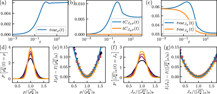
Figure 7: We consider the rotational flow Eq. (2) with $\Omega=3$ starting from steady-state initial conditions and use a Gaussian coarse-graining window Eq. (3) around $\mathbf{x}=(0,1)^{T}$ with width $h=0.5$. (a) Analytical result for the variance of the time-averaged density $\overline{\rho^{U}_{\mathbf{x}}(t)}$ multiplied by time $t$ as a function of $t$. At long times the variance approaches the large deviation variance in Eq. (76). (b) As in (a) but for the components of the correlation vector $\mathbf{C}^{\mathbf{x}\mathbf{x}}_{\mathbf{J}\rho}(t)$ as in Eqs. (45) and (61). (c) As in (a) but for the variances of the current components Eq. (52). (d) Simulation of the probability density function of the empirical density $\overline{\rho^{U}_{\mathbf{x}}}(t)$ assuming the parameters listed above. Colors of lines and symbols throughout denote $t=40,60,80,100$ from dark to bright. The simulated probability densities were obtained from histograms of $2\times 10^{4}$ trajectories for each set of parameters. (e) Parabolic approximation for the rate function with variance from Eq. (76) (line) and simulated rate function $I(\rho)=-\frac{1}{t}\ln P[\overline{\rho^{U}_{\mathbf{x}}}(t)=\rho]$ (symbols). The numerical value of the rate function at the mean $\rho=\langle\overline{\rho^{U}_{\mathbf{x}}}(t)\rangle_{\rm s}$ was subtracted. (f-g) As in (d-e) but for the $x$-component of the current $[\overline{\mathbf{J}^{U}_{\mathbf{x}}}]_{x}$ instead of the density $\overline{\rho^{U}_{\mathbf{x}}}$.

As already noted on several occasions, in the case of steady-state initial conditions the mean values of the time-averaged density and current are time-independent, see Eqs. (15),(17). The correlation and (co)variance results (Eqs. (23),(45),(49) with integral operator (22)) display a non-trivial temporal behavior dictated by the time integrals $\frac{1}{t}\!\int_{0}^{t}dt^{\prime}\left(1-\frac{t^{\prime}}{t}\right)$ over two-point densities $P_{\mathbf{z}}(\mathbf{z}^{\prime},t^{\prime})$.

In Fig. 7a-c we depict this time-dependent behavior for the two-dimensional rotational flow Eq. (2) for $\mathbf{x}=\mathbf{y}$. The short-time behavior can be obtained by analogy to the short-time expansion in the SM of [58]. Note that the short-time limit of fluctuations of time-integrated currents recently attracted much attention in the context of inference of dissipation, since in this limit the thermodynamic uncertainty relation becomes sharp [82, 83]. The long-time behavior shows that $\mathbf{C}(t),{\rm var}(t)\propto t^{-1}$, as expected from the central limit theorem (and large deviation theory) due to sufficiently many sufficiently uncorrelated visits of the window region. Accordingly, a serious problem is encountered in dimensions $\geq 2$ in the limit $h\to 0$ because diffusive trajectories do not hit points (for a detailed discussion see [58]).

The limit of $t\mathbf{C}(t),\,t{\rm var}(t)$ for large $t$ can be obtained as follows. We have $\int_{t^{\prime}}^{\infty}dt^{\prime\prime}[P_{\mathbf{y}}(\mathbf{x},t^{\prime\prime})-p_{\rm s}(\mathbf{x})]\to 0$ for $t^{\prime}\to\infty$ since $P_{\mathbf{y}}(\mathbf{x},t^{\prime})\overset{t^{\prime}\to\infty}{\longrightarrow}p_{\rm s}(\mathbf{x})$ and $\hat{\mathbf{j}}_{\mathbf{x}}P_{\mathbf{y}}(\mathbf{x},t^{\prime})\overset{t^{\prime}\to\infty}{\longrightarrow}{\mathbf{j}}_{\rm s}(\mathbf{x})$ with exponentially decaying deviations. This implies that for large $t$, we can replace $\frac{1}{t}\int_{0}^{t}dt^{\prime}\left(1-\frac{t^{\prime}}{t}\right)$ by $\frac{1}{t}\int_{0}^{\infty}dt^{\prime}$ in the integral operator (22). This replacement of integrals and the scaling are also confirmed by a spectral expansion (see e.g. [51] for spectral-theoretic results for the empirical density).

We now discuss the central-limit regime, which is contained in large deviation theory as small deviations from the mean. According to the central limit theorem (for not almost surely constant $U_{\mathbf{x}}^{h}$, and for finite variances (i.e. strictly positive $h$, see V)), the probability distributions $p(A_{t}=a)$ for $A_{t}=\overline{\rho^{U}_{\mathbf{x}}}(t)$ and $A_{t}=\overline{\mathbf{J}^{U}_{\mathbf{x}}}(t)$ become Gaussian for large $t$. This is contained in large deviation theory in terms of a parabola that locally (for $a\approx\mu$) approximates the rate function

$$I(a)=-\lim_{t\to\infty}\frac{1}{t}\ln p(A_{t}=a){\color[rgb]{0,0,0}\approx}\frac{(a-\mu)^{2}}{2\sigma^{2}_{A}},$$ (74)

where the mean $\mu$ is given by $\left\langle{\rho^{U}_{\mathbf{x}}(t)}\right\rangle_{\rm s}=\int d^{d}zU^{h}_{\mathbf{x}}(\mathbf{z})p_{\rm s}(\mathbf{z})$ and $\left\langle{\mathbf{J}^{U}_{\mathbf{x}}(t)}\right\rangle_{\rm s}=\int d^{d}zU^{h}_{\mathbf{x}}(\mathbf{z}){\mathbf{j}}_{\rm s}(\mathbf{z})$ (see Eqs. (15),(17)) and the large deviation variance $\sigma^{2}_{A}$ follows by the above arguments from Eqs. (23) and (49) for $\mathbf{x}=\mathbf{y}$ as in Eq. (61) as

$$\sigma^{2}_{\overline{\rho^{U}_{\mathbf{x}}}} \equiv\lim_{t\to\infty}t\,{\rm var}_{\rho}^{\mathbf{x}}(t)$$

$$=2\!\int_{0}^{\infty}\!\!\!\!\!\!dt^{\prime}\!\!\int\!\!d^{d}z\!\int\!\!d^{d}z^{\prime}U^{h}_{\mathbf{x}}(\mathbf{z})U^{h}_{\mathbf{x}}(\mathbf{z}^{\prime})$$

$$\quad\times\left[P_{\mathbf{z}^{\prime}}(\mathbf{z},t)-p_{\rm s}(\mathbf{z})p_{\rm s}(\mathbf{z}^{\prime})\right],$$ (75)

as well as

$$\sigma^{2}_{\overline{\mathbf{J}^{U}_{\mathbf{x}}}}\equiv\lim_{t\to\infty}t\,{\rm var}_{\mathbf{J}}^{\mathbf{x}}(t)=2{\rm Tr}\mathbf{D}\int d^{d}z\,[U^{h}_{\mathbf{x}}]^{2}(\mathbf{z})p_{\rm s}(\mathbf{z})$$

$$+2\int_{0}^{\infty}\!\!\!\!\!\!dt^{\prime}\!\!\int\!\!d^{d}z\!\int\!\!d^{d}z^{\prime}U^{h}_{\mathbf{x}}(\mathbf{z})U^{h}_{\mathbf{x}}(\mathbf{z}^{\prime})$$

$$\quad\times\left[\hat{\mathbf{j}}_{\mathbf{z}}\cdot{\hat{\mathbf{j}}}^{\ddagger}_{\mathbf{z}^{\prime}}P_{\mathbf{z}^{\prime}}(\mathbf{z},t)-{\mathbf{j}}_{\rm s}(\mathbf{z}){\mathbf{j}}_{\rm s}(\mathbf{z}^{\prime})\right].$$ (76)

For any Lebesgue integrable window function $U^{h}_{\mathbf{x}}$ (i.e. if the window size $h$ fulfills $h>0$), and in $d=1$ even for the delta-function, this variance is finite, and the central limit theorem applies as described above. The parabolic approximation for the rate function for a two dimensional system with finite window size $h>0$ is shown for the density $\overline{\rho^{U}_{\mathbf{x}}}(t)$ and current $\overline{\mathbf{J}^{U}_{\mathbf{x}}}(t)$ in Fig. 7e and g. The agreement of the simulation and the variance given by Eqs. (75)-(76) is readily confirmed.

If we instead take the limit of no coarse graining $h\to 0$ in multi-dimensional space $d\geq 2$, the variances diverge (see Eq. (51)). Fig. 8 depicts the distribution of the empirical density $\overline{\rho^{U}_{\mathbf{x}}}(t)$ in a fixed point $\mathbf{x}$ for different times $t$ and window sizes $h$. We see that the distribution becomes non-Gaussian for small $h$, in particular the most probable value departs from the mean and approaches $0$. Even though a Gaussian distribution is restored for longer times (see Fig. 8b), for even smaller window sizes the distribution again becomes non-Gaussian (see Fig. 8c). This behavior is not surprising since Gaussian distributions are only expected for sufficiently many (sufficiently uncorrelated) visits of the coarse graining window. For $h\to 0$ the recurrence time to return to the window diverges and thus for any finite $t$ one cannot expect a Gaussian distribution. Note that it is not clear whether a limit in distribution for $h\to 0$ of $\overline{\rho^{U}_{\mathbf{x}}}$ and $\overline{\mathbf{J}^{U}_{\mathbf{x}}}$ even exists. We hypothesize that, if the a limit $h\to 0$ of the distribution indeed exists, then it does so only as a scaling limit with $h\to 0$ and $t\to\infty$ simultaneously.

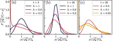
Figure 8: Simulation of the probability density function of the empirical density $\overline{\rho^{U}_{\mathbf{x}}}(t)$ for $\mathbf{x}=(0,1)^{T}$ and Gaussian window function $U^{h}_{\mathbf{x}}$ Eq. (3) with width $h$ for the two-dimensional driven Ornstein-Uhlenbeck process Eq. (2) with $\Omega=3$ with $\mathbf{x}_{0}$ starting from the steady state. The simulated probability density were obtained from histograms of $2\times 10^{5}$ trajectories for each set of parameters.

X Outlook beyond overdamped dynamics

In this section we give a brief outlook on the relevance of our findings in the limit $h\to 0$ for processes that are not described by purely overdamped dynamics. In particular, we highlight that although in physical systems the assumption of overdamped dynamics breaks down at very small time or length scales (which often may not be observable), the predicted divergence of fluctuations in the limit $h\to 0$ does not break down, or at least it remains true for sufficiently small finite $h$ that empirical densities and currents attain numerically very large values, i.e. effectively diverge. We emphasize that this section only establishes an outlook that underscores the experimental relevance of our approach, but does not contain quantitative theoretical results. Note that beyond the examples given here, the results in the limit $h\to 0$ also apply to Markov jump processes as illustrated in the Supplemental Material of [58].

To go beyond the assumption of Markovian overdamped motion assumed in Eq. (4), Fig. 9 depicts the fluctuations of the empirical density and current for two very different types of stochastic dynamics.

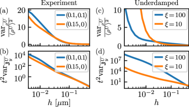
Figure 9: (a) Variance divided by squared mean of the empirical density and (b) variance of the empirical current with Gaussian coarse graining window (see Eqs (1),(3)) around $\mathbf{x}=(0.1,0.1)^{T}\mu$m and $\mathbf{x}=(0.15,0)^{T}\mu$m for $200$ experimental trajectories $(\mathbf{x}_{\tau}-\mathbf{x}_{0})_{\tau\leq 50\ \rm s}$ measured in particle tracking in living cells [85] with time-step $dt=0.1$ s and spatial resolution $10^{-3}\ \mu$m. (c) and (d) depict analogous results for underdamped dynamics simulated according to Eq. (77) for $1000$ trajectories with an Euler integration scheme with time step $dt=0.02$, total time $10$, initial positions $\mathbf{x}_{0}=(0,0)^{T}$ and Maxwellian initial velocities $\mathbf{v}_{0}$ (i.e. zero-mean Gaussian with variance $k_{B}T$), evaluated with Gaussian coarse graining window around $\mathbf{x}=(0.1,0)^{T}$. The observables in a,c and b,d relate to the predicted analytical curves in Figs. 3 and 6c, respectively, but now for completely different underlying dynamics. We note that processes not following an overdamped motion, in fact even non-Markovian processes, also seem to feature the divergence of fluctuations in the limit $h\to 0$, at least down to relevant small values of $h>0$ (larger than the resolution yet small enough to display impractically large fluctuations to be experimentally useful).

In Fig. 9a,b we evaluate the functionals in Eq. (1) with a Gaussian window function from Eq. (3) for particle-tracking data in living cells that was found to be well described by a two-state fractional Brownian motion [85, 86, 87]. The latter in particular is non-Markovian with subdiffusive anti-persistence on a given time scale. We observe that, even though the assumption of Markovian overdamped motion Eq. (4) is obviously violated (on some time and spatial scales), and thus the results of our work do not necessarily apply, we still find divergent fluctuations in the limit of small coarse graining scales $h$. Note that the resolution of the measurement is $h=10^{-3}\ \mu$m [85]. In Fig. 9a,b we observe that even for $h$ above this resolution limit the fluctuations approach impracticably large values. Therefore, we propose that in general scenarios (e.g. in this experimental set-up that extends way beyond the discussed overdamped dynamics) coarse graining empirical densities and currents may even in the case of very good statistics be necessary to obtain experimentally meaningful values with limited fluctuations.

In Fig. 9c,d we similarly evaluate the coarse-grained empirical density and current for two-dimensional underdamped harmonically confined Langevin dynamics with friction constant $\xi$ (setting for convenience the mass $m=1$ and temperature $k_{B}T=1$) simulated by integrating the equations of motion

$$d\mathbf{x}_{t} =\mathbf{v}_{t}dt$$

$$d\mathbf{v}_{t} =-\xi\mathbf{v}_{t}dt-\mathbf{x}_{t}dt+\sqrt{2\xi}d\mathbf{W}_{t}.$$ (77)

This dynamics exhibits persistence on time scales around or below $m/\xi$ (i.e. the ballistic regime). Again we find in Fig. 9c,d that the divergence predicted in the limit $h\to 0$ for overdamped dynamics is qualitatively preserved. The quantitative order of divergence will depend on the details of the process. We hypothesize that on time scales $h^{2}/D$ (with diffusion constant $D=k_{B}T/\xi$) that are smaller that $m/\xi$ the ballistic regime will cause deviations from the predicted divergence results in [58]. Following the arguments in Sec. V, the expressions will still diverge since the probability to hit points in $d\geq 2$-dimensional space becomes zero.

The influence of the details of the process, such as memory effects and ballistic transport, constitutes an interesting direction for future research that, however, goes beyond the scope of the present work. From the qualitative behavior found in Fig. 9 we may already conclude that the relevance of coarse graining empirical densities and currents to ensure finite and manageable fluctuations appears to be a quite general result, exceeding beyond the overdamped dynamics discussed in this work.

XI Conclusion

In this extended exposé accompanying the Letter [58] we presented the conceptual and technical background that is required to describe and understand the statistics of the empirical density and current of steady-state diffusions, which are central to statistical mechanics and thermodynamics on the level of individual trajectories. In order to gain deeper insight into the meaning of fluctuations of the empirical density and current we made use of a generalized time-reversal symmetry. We carried out a systematic analysis of the effect of a spatial coarse graining. A systematic variation of the coarse-graining scale in an a posteriori smoothing of trajectory data was proposed as an efficient method to infer bounds on a system’s dissipation. Moreover, we discussed symmetries in the statistics of the empirical current and density that arise as a result of the (generalized) time-reversal symmetry. Throughout the work we advocated the application of stochastic calculus, which is very powerful in the analysis of related problems and represents a more direct alternative to Feynman-Kac theory and path-integral methods. The technical background and concepts presented here may serve as a basis for forthcoming publications, including the generalization of the presented inference strategy to windows that are not centered at an individual point, as well as the use of the correlations result entering the CTUR inequality [56].

Acknowledgments—We thank Diego Krapf and Matthias Weiss for kindly providing traces from their particle-tracking experiments. Financial support from Studienstiftung des Deutschen Volkes (to C. D.) and the German Research Foundation (DFG) through the Emmy Noether Program GO 2762/1-2 (to A. G.) is gratefully acknowledged.

Appendix A Derivations in the limit of no coarse graining

We now take the limit to very small window sizes, i.e. the limit to no coarse graining, which will turn out to depend only on the properties of the two-point functions $P_{\mathbf{x}}(\mathbf{y},t^{\prime})$ for small time differences $t^{\prime}=t_{2}-t_{1}$. This allows us to derive the bounds in Eq. (51). We consider normalized window functions such that for a window size $h\to 0$ the window function becomes a delta distribution $U^{h}_{\mathbf{x}}(\mathbf{z})\to\delta(\mathbf{x}-\mathbf{z})$.

A.1 Density variance

For the variance of the density ${\rm var}^{\mathbf{x}}_{\rho}(t)\equiv\left\langle{\overline{\rho^{U}_{\mathbf{x}}}(t)^{2}}\right\rangle_{\rm s}-\left\langle{\overline{\rho^{U}_{\mathbf{x}}}(t)}\right\rangle_{\rm s}^{2}$, we have (see Eq. (23))

$${\rm var}^{\mathbf{x}}_{\rho}(t) =2\hat{\mathcal{I}}^{t,U}_{\mathbf{x}\mathbf{x}}[P_{\mathbf{z}^{\prime}}(\mathbf{z},t^{\prime})-p_{\rm s}(\mathbf{z})p_{\rm s}(\mathbf{z}^{\prime})].$$ (78)

For window size $h\to 0$ the mean remains finite such that $\hat{\mathcal{I}}^{t,U}_{\mathbf{x}\mathbf{x}}[p_{\rm s}(\mathbf{z})p_{\rm s}(\mathbf{z}^{\prime})]\overset{h\to 0}{\longrightarrow}-2p_{\rm s}(\mathbf{x})^{2}=O(h^{0})$. Now consider

$$\hat{\mathcal{I}}^{t,U}_{\mathbf{x}\mathbf{x}}[P_{\mathbf{z}^{\prime}}(\mathbf{z},t^{\prime})]=\frac{1}{t}\int_{0}^{t}dt^{\prime}\left(1-\frac{t^{\prime}}{t}\right)\int d^{d}z\int d^{d}z^{\prime}U^{h}_{\mathbf{x}}(\mathbf{z})U^{h}_{\mathbf{x}}(\mathbf{z}^{\prime})P_{\mathbf{z}^{\prime}}(\mathbf{z},t^{\prime}).$$ (79)

For $t^{\prime}>\varepsilon>0$, $P_{\mathbf{z}^{\prime}}(\mathbf{z},t^{\prime})$ is bounded and thus $\int d^{d}z\int d^{d}z^{\prime}U^{h}_{\mathbf{x}}(\mathbf{z})U^{h}_{\mathbf{x}}(\mathbf{z}^{\prime})P_{\mathbf{z}^{\prime}}(\mathbf{z},t^{\prime})$ is bounded using $\left\lvert\left\lvert P_{\mathbf{z}^{\prime}}(\mathbf{z},\varepsilon)\right\rvert\right\rvert_{\infty}=O(h^{0})$. Contributions diverging for $h\to 0$ can thus only come from the $t^{\prime}\to 0$ part of the integral, i.e. from small time differences $t^{\prime}=t_{2}-t_{1}$ (but not small absolute time $t$) in the Dyson series. To get the dominant divergent contribution, we can thus set $1-t^{\prime}/t\to 1$ and replace the two-point function $P_{\mathbf{z}^{\prime}}(\mathbf{z},t^{\prime})$ by the short time propagator $P_{\mathbf{y}}(\mathbf{z},t^{\prime})\to p_{\rm s}(\mathbf{z}^{\prime})G_{\rm short}(\mathbf{z},t^{\prime}|\mathbf{z}^{\prime})$ which reads (for simplicity take $\mathbf{D}(\mathbf{z})=D\mathbf{1}$, which we generalize later) [78]

$$G_{\rm short}(\mathbf{z},t^{\prime}|\mathbf{z}^{\prime}) =(4\pi Dt^{\prime})^{-d/2}\exp\left[-\frac{\left[\mathbf{z}-\mathbf{z}^{\prime}-F(\mathbf{z}^{\prime})t^{\prime}\right]^{2}}{4Dt^{\prime}}\right]$$

$$=(4\pi Dt^{\prime})^{-d/2}\exp\left[-\frac{\left[\mathbf{z}-\mathbf{z}^{\prime}\right]^{2}}{4Dt^{\prime}}+\frac{2(\mathbf{z}-\mathbf{z}^{\prime})\cdot\mathbf{F}(\mathbf{z}^{\prime})t^{\prime}}{4Dt^{\prime}}+O(t^{\prime})\right]$$

$$\overset{\mathbf{z}\approx\mathbf{z}^{\prime}}{\approx}(4\pi Dt^{\prime})^{-d/2}\left[1+\frac{1}{4D}(\mathbf{z}-\mathbf{z}^{\prime})\cdot\mathbf{F}(\mathbf{z}^{\prime})\right]\exp\left[-\frac{\left[\mathbf{z}-\mathbf{z}^{\prime}\right]^{2}}{4Dt^{\prime}}\right].$$ (80)

We write for $t^{\prime}\to 0,\mathbf{z}-\mathbf{z}^{\prime}\to\mathbf{0}$,

$$G_{\rm short,2} \equiv(4\pi Dt^{\prime})^{-d/2}\left[1+\frac{1}{2D}(\mathbf{z}-\mathbf{z}^{\prime})\cdot\mathbf{F}(\mathbf{z}^{\prime})\right]\exp\left[-\frac{\left[\mathbf{z}-\mathbf{z}^{\prime}\right]^{2}}{4Dt^{\prime}}\right]$$

$$G_{\rm short,3} \equiv(4\pi Dt^{\prime})^{-d/2}\exp\left[-\frac{\left[\mathbf{z}-\mathbf{z}^{\prime}\right]^{2}}{4Dt^{\prime}}\right],$$ (81)

where $G_{\rm short,2}$ can be replaced by $G_{\rm short,3}$ (since $\mathbf{z}-\mathbf{z}^{\prime}$ is small) if $G_{\rm short,3}$ does not give zero in the integrals..

For Gaussian window functions

$$U^{h}_{\mathbf{x}}(\mathbf{z})=(2\pi h^{2})^{-d/2}\exp\left[-\frac{(\mathbf{z}-\mathbf{x})^{2}}{2h^{2}}\right],$$ (82)

we obtain for the spatial integrals

$$\int d^{d}z\int d^{d}z^{\prime} U^{h}_{\mathbf{x}}(\mathbf{z})U^{h}_{\mathbf{x}}(\mathbf{z}^{\prime})G_{\rm short,3}(\mathbf{z},t^{\prime}|\mathbf{z}^{\prime})p_{\rm s}(\mathbf{z}^{\prime})$$

$$\simeq p_{\rm s}(\mathbf{x})\int d^{d}z\int d^{d}z^{\prime}U^{h}_{\mathbf{x}}(\mathbf{z})U^{h}_{\mathbf{x}}(\mathbf{z}^{\prime})G_{\rm short,3}(\mathbf{z},t^{\prime}|\mathbf{z}^{\prime})$$

$$=p_{\rm s}(\mathbf{x})(2\pi h^{2})^{-d}(4\pi Dt^{\prime})^{-d/2}\int d^{d}z\int d^{d}z^{\prime}\exp\left[-\frac{(\mathbf{z}-\mathbf{z})^{2}}{2h^{2}}-\frac{(\mathbf{z}^{\prime}-\mathbf{z})^{2}}{2h^{2}}-\frac{(\mathbf{z}-\mathbf{z}^{\prime})^{2}}{4Dt^{\prime}}\right]$$

$$=p_{\rm s}(\mathbf{x})(2\pi h^{2})^{-d}(4\pi Dt^{\prime})^{-d/2}\left(\int dx_{1}\int dy_{1}\exp\left[-\frac{x_{1}^{2}}{2h^{2}}-\frac{y_{1}^{2}}{2h^{2}}-\frac{(x_{1}-y_{1})^{2}}{4Dt^{\prime}}\right]\right)^{d}$$

$$=p_{\rm s}(\mathbf{x})\left[\frac{\sqrt{2Dh^{2}t^{\prime}+h^{4}}}{2\sqrt{\pi}h^{2}\sqrt{2Dt^{\prime}+h^{2}}\sqrt{\frac{Dt^{\prime}}{h^{2}}+1}}\right]^{d}$$

$$=p_{\rm s}(\mathbf{x})(4\pi)^{-d/2}(Dt^{\prime}+h^{2})^{-d/2}.$$ (83)

This implies, throughout denoting by $\simeq$ asymptotic equality in the limit $h\to 0$ (i.e. equality of the largest order),

$$\hat{\mathcal{I}}^{t,U}_{\mathbf{x}\mathbf{x}}[P_{\mathbf{z}^{\prime}}(\mathbf{z},t^{\prime})] \simeq(4\pi)^{-d/2}\frac{p_{\rm s}(\mathbf{x})}{t}\int_{0}^{t}dt^{\prime}(Dt^{\prime}+h^{2})^{-d/2}$$

$$=(4\pi)^{-d/2}\frac{p_{\rm s}(\mathbf{x})}{t}\times\begin{cases}-\frac{h^{2-d}}{D\left(1-\frac{d}{2}\right)}+\frac{\left(D+h^{2}\right)^{1-\frac{d}{2}}}{D\left(1-\frac{d}{2}\right)}&\text{for}\>d\neq 2\\ -\frac{\log{\left(h^{2}\right)}}{D}+\frac{\log{\left(D+h^{2}\right)}}{D}&\text{otherwise}\end{cases}$$

$$\simeq(4\pi)^{-d/2}\frac{2p_{\rm s}(\mathbf{x})}{Dt}\times\begin{cases}\frac{h^{2-d}}{d-2}&\text{for}\>d>2\\ -\log{\left(h\right)}&\text{for}\>d=2\end{cases}\ .$$ (84)

This gives for Gaussian $U$ with width $h$ the result

$$\text{var}^{\mathbf{x}}_{\rho}(t)\overset{h\to 0}{\simeq}(4\pi)^{-d/2}\frac{4p_{\rm s}(\mathbf{x})}{Dt}\times\begin{cases}\frac{h^{2-d}}{d-2}&\text{for}\>d>2\\ -\log{\left(h\right)}&\text{for}\>d=2\end{cases},$$ (85)

where only the numerical prefactor changes if we choose other indicator functions, since the relevant part (close to $\mathbf{x}$) of any finite size window function can be bounded from above and below by Gaussian window functions.

To extend to general diffusion matrices $\mathbf{D}(\mathbf{z})$, we first note that for $h\to 0$ only the local diffusion matrix $\mathbf{D}(\mathbf{x})$ at position $\mathbf{x}$ will enter the result, and, if the local $\mathbf{D}(\mathbf{x})$ is not isotropic we transform to coordinates where the diffusion matrix is diagonal, $\mathbf{D}(\mathbf{x})={\rm diag}(D_{1}(\mathbf{x}),\dots,D_{d}(\mathbf{x}))$. One can check this by Taylor expanding around $\mathbf{x}$ in $h$ in the local coordinate frame, isolating the leading order term, keeping in mind that $\mathbf{D}(\mathbf{z})$ was assumed to be smooth. In the local coordinates we then need to evaluate the integral

$$\int_{0}^{t}dt^{\prime}\prod_{i=1}^{d}(D_{i}(\mathbf{x})t^{\prime}+h^{2})^{-1/2},$$ (86)

whose integrand can be bounded by

$$(\max_{j}(D_{j}(\mathbf{x}))t^{\prime}+h^{2})^{-1/2}\leq(D_{i}(\mathbf{x})t^{\prime}+h^{2})^{-1/2}\leq(\min_{j}(D_{j}(\mathbf{x}))t^{\prime}+h^{2})^{-1/2},$$ (87)

implying that in the final result $D$ in Eq. (85) can be replaced by $\tilde{D}(\mathbf{x})\in[\min(D_{i}(\mathbf{x})),\max(D_{i}(\mathbf{x}))]$,

$$\text{var}^{\mathbf{x}}_{\rho}(t)\overset{h\to 0}{\simeq}(4\pi)^{-d/2}\frac{4p_{\rm s}(\mathbf{x})}{\tilde{D}(\mathbf{x})t}\times\begin{cases}\frac{h^{2-d}}{d-2}&\text{for}\>d>2\\ -\log{\left(h\right)}&\text{for}\>d=2\end{cases}.$$ (88)

The entries $D_{i}(\mathbf{x})$ of the diagonalized $\mathbf{D}(\mathbf{x})$ are the eigenvalues, hence in general $\tilde{D}(\mathbf{x})\in[\lambda(\mathbf{x})_{\rm min},\lambda(\mathbf{x})_{\rm max}]$ is bounded by the lowest and highest eigenvalues $\lambda(\mathbf{x})_{\rm min}$ and $\lambda(\mathbf{x})_{\rm max}$ of the matrix $\mathbf{D}(\mathbf{x})$. This proves the density variance result in Eq. (51).

A.2 Correlation of current and density

Now consider the small-window limit for correlations with $\mathbf{x}=\mathbf{y}$ defined as $\mathbf{C}_{\mathbf{J}\rho}^{\mathbf{x}\mathbf{x}}(t)\equiv\left\langle{\overline{\mathbf{J}^{U}_{\mathbf{x}}}(t)\overline{\rho^{U}_{\mathbf{x}}}(t)}\right\rangle_{\rm s}-\left\langle{\overline{\mathbf{J}^{U}_{\mathbf{x}}}(t)}\right\rangle_{\rm s}\left\langle{\overline{\rho^{U}_{\mathbf{x}}}(t)}\right\rangle_{\rm s}$, given according to Eq. (45) by

$$\mathbf{C}_{\mathbf{J}\rho}^{\mathbf{x}\mathbf{x}}(t)= \hat{\mathcal{I}}^{t,U}_{\mathbf{x}\mathbf{x}}\left[\hat{\mathbf{j}}_{\mathbf{z}}P_{\mathbf{z}^{\prime}}(\mathbf{z},t^{\prime})+{\hat{\mathbf{j}}}^{\ddagger}_{\mathbf{z}}P_{\mathbf{z}}(\mathbf{z}^{\prime},t^{\prime})-2{\mathbf{j}}_{\rm s}(\mathbf{z})p_{\rm s}(\mathbf{z}^{\prime})\right].$$ (89)

Recall that $\hat{\mathbf{j}}_{\mathbf{z}}=\mathbf{F}(\mathbf{z})-\mathbf{D}(\mathbf{z})\nabla_{\mathbf{z}}$. As always the term involving the mean values is finite for $h\to 0$. We first look at $\hat{\mathcal{I}}^{t,U}_{\mathbf{x}\mathbf{x}}[\hat{\mathbf{j}}_{\mathbf{z}}P_{\mathbf{z}^{\prime}}(\mathbf{z},t^{\prime})]$, again first for constant isotropic diffusion $\mathbf{D}(\mathbf{z})=D\mathbf{1}$.

Here we have to use $G_{\rm short,2}$, see Eq. (81), since the integrals over $G_{\rm short,3}$ vanish. Hence consider

$$\hat{\mathcal{I}}^{t,U}_{\mathbf{x}\mathbf{x}}[\hat{\mathbf{j}}_{\mathbf{z}}P_{\mathbf{z}^{\prime}}(\mathbf{z},t^{\prime})] =\frac{1}{t}\int_{0}^{t}dt^{\prime}\left(1-\frac{t^{\prime}}{t}\right)\int d^{d}z\int d^{d}z^{\prime}U^{h}_{\mathbf{x}}(\mathbf{z})U^{h}_{\mathbf{x}}(\mathbf{z}^{\prime})\hat{\mathbf{j}}_{\mathbf{z}}P_{\mathbf{z}^{\prime}}(\mathbf{z},t^{\prime})$$

$$\simeq\frac{p_{\rm s}(\mathbf{x})}{t}\int_{0}^{t}dt^{\prime}\int d^{d}z\int d^{d}z^{\prime}U^{h}_{\mathbf{x}}(\mathbf{z})U^{h}_{\mathbf{x}}(\mathbf{z}^{\prime})[\mathbf{F}(\mathbf{z})-D\nabla_{\mathbf{z}}]G_{\rm short,2}(\mathbf{z},t^{\prime}|\mathbf{z}^{\prime}),$$ (90)

where we can use $\hat{\mathcal{I}}^{t,U}_{\mathbf{x}\mathbf{x}}[\mathbf{F}(\mathbf{z})P_{\mathbf{z}^{\prime}}(\mathbf{z},t^{\prime})]\simeq\mathbf{F}(\mathbf{x})\hat{\mathcal{I}}^{t,U}_{\mathbf{x}\mathbf{x}}[P_{\mathbf{z}^{\prime}}(\mathbf{z},t^{\prime})]\simeq\mathbf{F}(\mathbf{x})\times\eqref{divergence_return_integral}$ and we compute

$$\nabla_{\mathbf{z}}G_{\rm short,2}(\mathbf{z},t^{\prime}|\mathbf{z}^{\prime})$$

$$=(4\pi Dt^{\prime})^{-d/2}\left[1+\frac{1}{2D}(\mathbf{z}-\mathbf{z}^{\prime})\cdot\mathbf{F}(\mathbf{z}^{\prime})\right]\nabla_{\mathbf{z}}\exp\left[-\frac{\left[\mathbf{z}-\mathbf{z}^{\prime}\right]^{2}}{4Dt^{\prime}}\right]+(4\pi Dt^{\prime})^{-d/2}\frac{\mathbf{F}(\mathbf{z}^{\prime})}{2D}\exp\left[-\frac{\left[\mathbf{z}-\mathbf{z}^{\prime}\right]^{2}}{4Dt^{\prime}}\right]$$

$$=-(4\pi Dt^{\prime})^{-d/2}\left[1+\frac{1}{2D}(\mathbf{z}-\mathbf{z}^{\prime})\cdot\mathbf{F}(\mathbf{z}^{\prime})\right]\frac{\mathbf{z}-\mathbf{z}^{\prime}}{2Dt^{\prime}}\exp\left[-\frac{\left[\mathbf{z}-\mathbf{z}^{\prime}\right]^{2}}{4Dt^{\prime}}\right]+(4\pi Dt^{\prime})^{-d/2}\frac{\mathbf{F}(\mathbf{z}^{\prime})}{2D}\exp\left[-\frac{\left[\mathbf{z}-\mathbf{z}^{\prime}\right]^{2}}{4Dt^{\prime}}\right].$$ (91)

By symmetry, the spatial integrals over $(\mathbf{z}-\mathbf{z}^{\prime})\exp\left[-\frac{\left[\mathbf{z}-\mathbf{z}^{\prime}\right]^{2}}{4Dt^{\prime}}\right]$ vanish and we are left to compute

$$-D\int d^{d}z\int d^{d}z^{\prime}U^{h}_{\mathbf{x}}(\mathbf{z})U^{h}_{\mathbf{x}}(\mathbf{z}^{\prime})\nabla_{\mathbf{z}}G_{\rm short,2}(\mathbf{z},t^{\prime}|\mathbf{z}^{\prime})$$

$$\simeq-D(4\pi Dt^{\prime})^{-d/2}\int d^{d}x\int d^{d}yU(\mathbf{x})U(\mathbf{y})\left(-\frac{[(\mathbf{x}-\mathbf{y})\cdot\mathbf{F}(\mathbf{y})](\mathbf{x}-\mathbf{y})}{4D^{2}t^{\prime}}+\frac{\mathbf{F}(\mathbf{z}^{\prime})}{2D}\right)\exp\left[-\frac{\left[\mathbf{z}-\mathbf{z}^{\prime}\right]^{2}}{4Dt^{\prime}}\right],$$ (92)

where the second term gives $-\frac{1}{2}\mathbf{F}(\mathbf{x})\hat{\mathcal{I}}^{t,U}_{\mathbf{x}\mathbf{x}}[P_{\mathbf{z}^{\prime}}(\mathbf{z},t^{\prime})]$. The remaining term, noting that $\mathbf{F}(\mathbf{z}^{\prime})\simeq\mathbf{F}(\mathbf{x})$ and integrating out all directions except $k$ for the $F_{k}(\mathbf{x})$ component (by symmetry $(z_{i}-z^{\prime}_{i})(z_{j}-z^{\prime}_{j})$ integrates to zero if $i\neq j$), becomes

$$\frac{(4\pi Dt^{\prime})^{-d/2}}{4Dt^{\prime}}\int d^{d}z\int d^{d}z^{\prime}U^{h}_{\mathbf{x}}(\mathbf{z})U^{h}_{\mathbf{x}}(\mathbf{z}^{\prime})[(\mathbf{z}-\mathbf{z}^{\prime})\cdot\mathbf{F}(\mathbf{x})](\mathbf{z}-\mathbf{z}^{\prime})\exp\left[-\frac{\left[\mathbf{z}-\mathbf{z}^{\prime}\right]^{2}}{4Dt^{\prime}}\right]$$

$$=\frac{\mathbf{F}(\mathbf{x})}{4Dt^{\prime}}\int dz_{1}\int dz^{\prime}_{1}U^{1}(z_{1})U^{1}(z^{\prime}_{1})(z_{1}-z^{\prime}_{1})^{2}G_{\rm short,3,one-dim}(z_{1},t^{\prime}|z^{\prime}_{1})$$

$$=\frac{\mathbf{F}(\mathbf{x})}{4Dt^{\prime}}\frac{Dh^{2}t^{\prime}}{\sqrt{\pi}\left(Dt^{\prime}+h^{2}\right)^{\frac{3}{2}}}$$

$$=\frac{\mathbf{F}(\mathbf{x})h^{2}}{4\sqrt{\pi}\left(Dt^{\prime}+h^{2}\right)^{\frac{3}{2}}}.$$ (93)

This term is subdominant as we see from the time integral

$$\hat{\mathcal{I}}^{t,U}_{\mathbf{x}\mathbf{x}}[-D\nabla_{\mathbf{z}}P_{\mathbf{z}^{\prime}}(\mathbf{z},t^{\prime})] \simeq-\frac{\mathbf{F}(\mathbf{x})}{2}\hat{\mathcal{I}}^{t,U}_{\mathbf{x}\mathbf{x}}[P_{\mathbf{z}^{\prime}}(\mathbf{z},t^{\prime})]+\frac{p_{\rm s}(\mathbf{x})\mathbf{F}(\mathbf{x})h^{2}}{4\sqrt{\pi}t}\underbrace{\int_{0}^{t}dt^{\prime}\left(Dt^{\prime}+h^{2}\right)^{-\frac{3}{2}}}_{h^{-1}}$$

$$\simeq-\frac{\mathbf{F}(\mathbf{x})}{2}\hat{\mathcal{I}}^{t,U}_{\mathbf{x}\mathbf{x}}[P_{\mathbf{z}^{\prime}}(\mathbf{z},t^{\prime})].$$ (94)

Hence, overall we get

$$\hat{\mathcal{I}}^{t,U}_{\mathbf{x}\mathbf{x}}[\hat{\mathbf{j}}_{\mathbf{z}}P_{\mathbf{z}^{\prime}}(\mathbf{z},t^{\prime})] =\frac{\mathbf{F}(\mathbf{x})}{2}\hat{\mathcal{I}}^{t,U}_{\mathbf{x}\mathbf{x}}[P_{\mathbf{z}^{\prime}}(\mathbf{z},t^{\prime})].$$ (95)

The generalization to non-constant or non-isotropic $\mathbf{D}(\mathbf{z})$ only changes $\hat{\mathcal{I}}^{t,U}_{\mathbf{x}\mathbf{x}}[P_{\mathbf{z}^{\prime}}(\mathbf{z},t^{\prime})]$ but Eq. (95) is retained.

Now consider $\hat{\mathcal{I}}^{t,U}_{\mathbf{x}\mathbf{x}}[{\hat{\mathbf{j}}}^{\ddagger}_{\mathbf{z}}P_{\mathbf{z}}(\mathbf{z}^{\prime},t^{\prime})]$. Since this involves derivatives of both $G$ and $p_{\rm s}$ (at the initial point) we instead take the form ${\hat{\mathbf{j}}}^{\ddagger}_{\mathbf{z}}={\mathbf{j}}_{\rm s}(\mathbf{z})/p_{\rm s}(\mathbf{z})+Dp_{\rm s}(\mathbf{z})\nabla_{\mathbf{z}}p_{\rm s}(\mathbf{z})^{-1}$ such that ${\hat{\mathbf{j}}}^{\ddagger}_{\mathbf{z}}P_{\mathbf{z}}(\mathbf{z}^{\prime},t^{\prime})=[{\mathbf{j}}_{\rm s}(\mathbf{z})+Dp_{\rm s}(\mathbf{z})\nabla_{\mathbf{z}}]G(\mathbf{z}^{\prime},t^{\prime}|\mathbf{z})$ giving

$$\hat{\mathcal{I}}^{t,U}_{\mathbf{x}\mathbf{x}}[{\hat{\mathbf{j}}}^{\ddagger}_{\mathbf{z}}P_{\mathbf{z}}(\mathbf{z}^{\prime},t^{\prime})] =\frac{1}{t}\int_{0}^{t}dt^{\prime}\left(1-\frac{t^{\prime}}{t}\right)\int d^{d}z\int d^{d}z^{\prime}U^{h}_{\mathbf{x}}(\mathbf{z})U^{h}_{\mathbf{x}}(\mathbf{z}^{\prime})[{\mathbf{j}}_{\rm s}(\mathbf{z})+Dp_{\rm s}(\mathbf{z})\nabla_{\mathbf{z}}]G(\mathbf{z}^{\prime},t^{\prime}|\mathbf{z})$$

$$\simeq\frac{{\mathbf{j}}_{\rm s}(\mathbf{x})}{p_{\rm s}(\mathbf{x})}\hat{\mathcal{I}}^{t,U}_{\mathbf{x}\mathbf{x}}[P_{\mathbf{z}}(\mathbf{z}^{\prime},t^{\prime})]+Dp_{\rm s}(\mathbf{x})\int_{0}^{t}dt^{\prime}\int d^{d}z\int d^{d}z^{\prime}U^{h}_{\mathbf{x}}(\mathbf{z})U^{h}_{\mathbf{x}}(\mathbf{z}^{\prime})\nabla_{\mathbf{z}}G_{\rm short,2}(\mathbf{z}^{\prime},t^{\prime}|\mathbf{z}),$$ (96)

where (note that $G_{\rm short,3}(\mathbf{z},t^{\prime}|\mathbf{z}^{\prime})=G_{\rm short,3}(\mathbf{z}^{\prime},t^{\prime}|\mathbf{z})$)

$$\nabla_{\mathbf{z}}G_{\rm short,2}(\mathbf{z}^{\prime},t^{\prime}|\mathbf{z})$$

$$=(4\pi Dt^{\prime})^{-d/2}\left[1+\frac{1}{2D}(\mathbf{z}^{\prime}-\mathbf{z})\cdot\mathbf{F}(\mathbf{z}^{\prime})\right]\nabla_{\mathbf{z}}\exp\left[-\frac{\left[\mathbf{z}-\mathbf{z}^{\prime}\right]^{2}}{4Dt^{\prime}}\right]+(4\pi Dt^{\prime})^{-d/2}\frac{-\mathbf{F}(\mathbf{z})}{2D}\exp\left[-\frac{\left[\mathbf{z}-\mathbf{z}^{\prime}\right]^{2}}{4Dt^{\prime}}\right]$$

$$=-(4\pi Dt^{\prime})^{-d/2}\left[1+\frac{1}{2D}(\mathbf{z}-\mathbf{z}^{\prime})\cdot\mathbf{F}(\mathbf{z}^{\prime})\right]\frac{\mathbf{z}-\mathbf{z}^{\prime}}{2Dt^{\prime}}\exp\left[-\frac{\left[\mathbf{z}-\mathbf{z}^{\prime}\right]^{2}}{4Dt^{\prime}}\right]-\frac{\mathbf{F}(\mathbf{z}^{\prime})}{2D}G_{\rm short,3}(\mathbf{z}^{\prime},t^{\prime}|\mathbf{z}).$$ (97)

As before, asymptotically only the last term contributes, giving

$$\hat{\mathcal{I}}^{t,U}_{\mathbf{x}\mathbf{x}}[{\hat{\mathbf{j}}}^{\ddagger}_{\mathbf{z}}P_{\mathbf{z}}(\mathbf{z}^{\prime},t^{\prime})] \simeq\frac{{\mathbf{j}}_{\rm s}(\mathbf{x})}{p_{\rm s}(\mathbf{x})}\hat{\mathcal{I}}^{t,U}_{\mathbf{x}\mathbf{x}}[P_{\mathbf{z}}(\mathbf{z}^{\prime},t^{\prime})]+Dp_{\rm s}(\mathbf{x})\int_{0}^{t}dt^{\prime}\int d^{d}z\int d^{d}z^{\prime}U^{h}_{\mathbf{x}}(\mathbf{z})U^{h}_{\mathbf{x}}(\mathbf{z}^{\prime})\nabla_{\mathbf{z}}G_{\rm short,2}(\mathbf{z}^{\prime},t^{\prime}|\mathbf{z})$$

$$\simeq\frac{{\mathbf{j}}_{\rm s}(\mathbf{x})}{p_{\rm s}(\mathbf{x})}\hat{\mathcal{I}}^{t,U}_{\mathbf{x}\mathbf{x}}[P_{\mathbf{z}}(\mathbf{z}^{\prime},t^{\prime})]+Dp_{\rm s}(\mathbf{x})\int_{0}^{t}dt^{\prime}\int d^{d}z\int d^{d}z^{\prime}U^{h}_{\mathbf{x}}(\mathbf{z})U^{h}_{\mathbf{x}}(\mathbf{z}^{\prime})\frac{-\mathbf{F}(\mathbf{z}^{\prime})}{2D}G_{\rm short,3}(\mathbf{z}^{\prime},t^{\prime}|\mathbf{z})$$

$$\simeq\left[\frac{{\mathbf{j}}_{\rm s}(\mathbf{x})}{p_{\rm s}(\mathbf{x})}-\frac{\mathbf{F}(\mathbf{x})}{2}\right]\hat{\mathcal{I}}^{t,U}_{\mathbf{x}\mathbf{x}}[P_{\mathbf{z}}(\mathbf{z}^{\prime},t^{\prime})].$$ (98)

Overall, this gives for the correlations (having the same form for anisotropic diffusion)

$$\mathbf{C}_{\mathbf{J}\rho}^{\mathbf{x}\mathbf{x}}(t)\overset{h\to 0}{\simeq}\frac{{\mathbf{j}}_{\rm s}(\mathbf{x})}{p_{\rm s}(\mathbf{x})}\hat{\mathcal{I}}^{t,U}_{\mathbf{x}\mathbf{x}}[P_{\mathbf{z}}(\mathbf{z}^{\prime},t^{\prime})]\simeq\frac{{\mathbf{j}}_{\rm s}(\mathbf{x})}{2p_{\rm s}(\mathbf{x})}\text{var}^{\mathbf{x}}_{\rho}(t).$$ (99)

This proves the correlation result in Eq. (51).

A.3 Current variance

We now turn to the current variance, see Eq. (49) for $\mathbf{x}=\mathbf{y}$,

$$\text{var}^{\mathbf{x}}_{\mathbf{J}}(t)=\frac{2}{t}\int d^{d}z{\rm Tr}\mathbf{D}(\mathbf{z})U^{h}_{\mathbf{x}}(\mathbf{z})U^{h}_{\mathbf{x}}(\mathbf{z})p_{\rm s}(\mathbf{z})+2\hat{\mathcal{I}}^{t,U}_{\mathbf{x}\mathbf{x}}\left[\hat{\mathbf{j}}_{\mathbf{z}}\cdot{\hat{\mathbf{j}}}^{\ddagger}_{\mathbf{z}^{\prime}}P_{\mathbf{z}^{\prime}}(\mathbf{z},t^{\prime})-{\mathbf{j}}_{\rm s}(\mathbf{z})\cdot{\mathbf{j}}_{\rm s}(\mathbf{z}^{\prime})\right].$$ (100)

The first term for $h\to 0$ gives

$$\frac{2{\rm Tr}\mathbf{D}(\mathbf{z})}{t}\int d^{d}xU^{h}_{\mathbf{x}}(\mathbf{z})U^{h}_{\mathbf{x}}(\mathbf{z})p_{\rm s}(\mathbf{z})\simeq\frac{2{\rm Tr}\mathbf{D}(\mathbf{x})}{t}p_{\rm s}(\mathbf{x})U^{h}_{\mathbf{x}}(\mathbf{x}),$$ (101)

where $U^{h}_{\mathbf{x}}(\mathbf{x})\propto h^{-d}$ is the height of the delta-function approximation, e.g. $U^{h}_{\mathbf{x}}(\mathbf{x})=(2\pi)^{-d/2}h^{-d}$ for Gaussian $U^{h}_{\mathbf{x}}$. In the derivation (see Sec. IV) this term occurred from cross correlations $dW_{t_{1}}dW_{t_{1}}=dt^{\prime}\neq 0$ in the noise part, hence it can be seen to come from zero time-differences $t^{\prime}=t_{2}-t_{1}=0$. Such a term does not appear in the density variance or density-current correlation since there $dt_{1}dt_{2}=0$ and $dt_{1}dW_{t_{2}}=0$ would occur instead of $dW_{t_{1}}dW_{t_{2}}$.

Due to the fast $h^{-d}$ divergence, the dominant limit does not depend on terms with no or only one derivative since they were shown to scale at most as $h^{2-d}$. The only new term is the second derivative for which we see that

$$\int_{0}^{t}dt^{\prime}D\nabla_{\mathbf{z}}\cdot(-\nabla_{\mathbf{z}^{\prime}})G_{\text{short,3}}(\mathbf{z},t^{\prime}|\mathbf{z}^{\prime})$$

$$=\int_{0}^{t}D\nabla_{\mathbf{z}}^{2}G_{\text{short,3}}(\mathbf{z},t^{\prime}|\mathbf{z}^{\prime})$$

$$=\int_{0}^{t}dt^{\prime}\partial_{t^{\prime}}G_{\text{short,3}}(\mathbf{z},t^{\prime}|\mathbf{z}^{\prime})$$

$$=\left[G_{\text{short,3}}(\mathbf{z},t^{\prime}|\mathbf{z}^{\prime})\right]_{0}^{t}$$

$$=G_{\text{short,3}}(\mathbf{z},t|\mathbf{z}^{\prime})-\delta(\mathbf{z}-\mathbf{z}^{\prime}),$$ (102)

such that

$$\hat{\mathcal{I}}^{t,U}_{\mathbf{x}\mathbf{x}}\left[\hat{\mathbf{j}}_{\mathbf{z}}\cdot{\hat{\mathbf{j}}}^{\ddagger}_{\mathbf{z}^{\prime}}P_{\mathbf{z}^{\prime}}(\mathbf{z},t^{\prime})\right] \simeq-D^{2}\frac{p_{\rm s}(\mathbf{x})}{t}\int_{0}^{t}dt^{\prime}\int d^{d}z\int d^{d}z^{\prime}U^{h}_{\mathbf{x}}(\mathbf{z})U^{h}(\mathbf{z})\nabla_{\mathbf{z}}\cdot\nabla_{\mathbf{z}^{\prime}}G_{\text{short,3}}(\mathbf{z},t^{\prime}|\mathbf{z}^{\prime})$$

$$\simeq-D\frac{p_{\rm s}(\mathbf{x})}{t}\int d^{d}z\int d^{d}z^{\prime}U^{h}_{\mathbf{x}}(\mathbf{z})U^{h}(\mathbf{z}^{\prime})\delta(\mathbf{z}-\mathbf{z}^{\prime})$$

$$\simeq-D\frac{p_{\rm s}(\mathbf{x})}{t}U^{h}(\mathbf{x}).$$ (103)

For non-isotropic and possibly non-constant $\mathbf{D}(\mathbf{z})\neq D\mathbf{1}$, we again note that for $h\to 0$ only $\mathbf{D}(\mathbf{z})$ at $\mathbf{z}=\mathbf{x}$ matters, and move to the basis where $\mathbf{D}=\mathbf{D}(\mathbf{x})$ is diagonal, where we have

$$D^{2}\nabla_{\mathbf{z}}\cdot\nabla_{\mathbf{z}^{\prime}}\longrightarrow\sum_{i=1}^{d}D_{i}^{2}\partial_{z_{i}}\partial_{z_{i^{\prime}}}.$$ (104)

The operator we need is $\nabla_{\mathbf{z}}\mathbf{D}\nabla_{\mathbf{z}^{\prime}}=\sum_{i}D_{i}\partial_{z_{i}}\partial_{z_{i^{\prime}}}$ so we bound one of the $D_{i}$ in $D_{i}^{2}$ by $D^{\prime}\in[\min(D_{i}),\max(D_{i})]$ such that we get

$$\hat{\mathcal{I}}^{t,U}_{\mathbf{x}\mathbf{x}}\left[\hat{\mathbf{j}}_{\mathbf{z}}\cdot{\hat{\mathbf{j}}}^{\ddagger}_{\mathbf{z}^{\prime}}P_{\mathbf{z}^{\prime}}(\mathbf{z},t^{\prime})\right] \simeq-D^{\prime}\frac{p_{\rm s}(\mathbf{x})}{t}U^{h}(\mathbf{x}).$$ (105)

Since ${\rm Tr}\mathbf{D}=\sum_{i}D_{i}$ we have $\tilde{D}^{\prime}\equiv\frac{{\rm Tr}\mathbf{D}-D^{\prime}}{d-1}\in[\min(D_{i}),\max(D_{i})]$ and we can write

$$\text{var}^{\mathbf{x}}_{\mathbf{J}}(t) \simeq\frac{2{\rm Tr}\mathbf{D}}{t}p_{\rm s}(\mathbf{x})U^{h}(\mathbf{x})-2D^{\prime}\frac{p_{\rm s}(\mathbf{x})}{t}U^{h}(\mathbf{x})=\frac{2\tilde{D}^{\prime}}{t}p_{\rm s}(\mathbf{x})(d-1)U(\mathbf{x}),$$ (106)

where $U(\mathbf{x})\propto h^{-d}$. This proves the current variance result in Eq. (51). Thus, we see that the current fluctuations diverge for $h\to 0$, except in one-dimensional space where $d-1=0$.

A.4 Limit of no coarse graining in the one-dimensional case

In the one-dimensional case, the variance of empirical density and current remain finite for $h\to 0$ which allows to take the limit to $U^{h=0}_{x}(x^{\prime})=\delta(x-x^{\prime})$. In terms of the stochastic integrals, the one-dimensional case is much simpler, since any one-dimensional function $U^{h}_{x}(x^{\prime})$ possesses an antiderivative – a primitive function $\mathcal{U}^{h}_{x}(x^{\prime})=\int^{x^{\prime}}U^{h}_{x}(x^{\prime\prime})dx^{\prime\prime}$ such that $U^{h}_{x}(x^{\prime})=\partial_{x^{\prime}}\mathcal{U}_{x}(x^{\prime}).$ This implies for the Stratonovich integral that

$$t\overline{J^{U}_{x}}(t)=\int_{0}^{t}U^{h}_{x}(x_{\tau})\circ dx_{\tau}=\mathcal{U}_{x}(x_{t})-\mathcal{U}_{x}(x_{0}).$$ (107)

Thus, the stochastic current is no longer a functional but only a function of the initial- and end-point of the trajectory. Its moments are directly accessible, e.g.

$$\left\langle{[\overline{J^{U}_{x}}(t)]^{2}}\right\rangle_{\rm s}=\frac{1}{t^{2}}\left\langle{\left[\mathcal{U}_{x}(x_{t})-\mathcal{U}_{x}(x_{0})\right]^{2}}\right\rangle_{\rm s}=\frac{1}{t^{2}}\int dz\int dz^{\prime}\left[\mathcal{U}_{x}(z)-\mathcal{U}_{x}(z^{\prime})\right]^{2}P_{z^{\prime}}(z,t).$$ (108)

If $U$ is Gaussian, then $\mathcal{U}_{x}$ is the error function such that $\left[\mathcal{U}_{x}(x)-\mathcal{U}_{x}(y)\right]^{2}\leq 1$ and thus $\left\langle{[\overline{J^{U}_{x}}(t)]^{2}}\right\rangle_{\rm s}\leq 1/t^{2}$. This also holds in the limit of a delta function where the primitive function becomes a Heaviside step function and we get that the current can only be $0$ or $\pm t^{-2}$, see Fig. 10. The current defined with a delta function at $x$ simply counts the net number of crossing through $x$ such that all crossings except maybe one cancel out. Note that the reasoning above only holds for the current defined with a Stratonovich integral—the same definition with an Itô or anti-Itô integral would give a divergent current for the delta function.

To obtain a $1/t$-term as in large deviations one would need to have a steady-state current which could e.g. be achieved by generalizing to periodic boundary conditions. Then the current would depend on the initial and final point and, in addition, also on the net number of crossings of the full interval between the boundaries of the system.

Fig. 10 shows the time-integrated density and current, i.e. the empirical density and current Eq. (1) multiplied by the total time $t$. Fluctuations remain in the same order of magnitude for $h\to 0$ (see Fig. 10c,e). We see that the time-integrated current is bounded by $1$ which is due to the fact that it simply counts the net number of crossings. According to Eq. (107) it only depends on the initial-point $x_{0}$ and end-point $x_{t}$, in this case $x_{10}$.

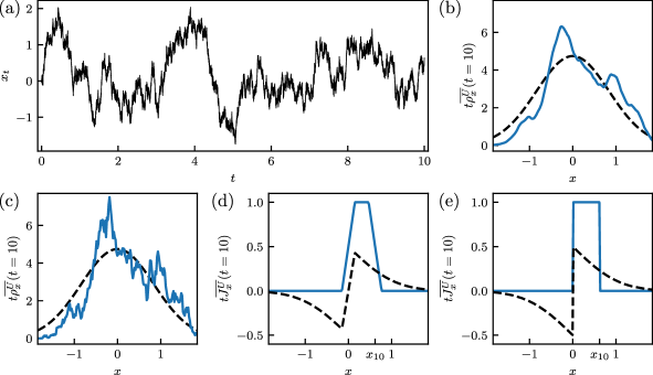
Figure 10: (a) One-dimensional Brownian motion in a harmonic potential (see Eq. (2) in 1d with parameters $r=\sqrt{2}$ and $D=1$) starting at $x_{0}=0$ and ending at $x_{10}=0.62$. (b) Time-integrated density of the trajectory in (a) as a function of $x$ for normalized window function $U^{h}_{x}(x^{\prime})=h^{-1}\mathbbm{1}_{\left\lvert x-x^{\prime}\right\rvert\leq h/2}$ with width $h=0.3$. The dashed line shows the expectation value of the time-integrated density conditioned on $\mathbf{x}_{0}=0$. (c) As in (b) with width $h=0.001$. (d) Time-integrated current for window as in (b) width $h=0.3$. The dashed line shows the expectation value of the time-integrated current conditioned on $\mathbf{x}_{0}=0$. (e) As in (d) for width $h=0.001$.