Abstract

Decentralized learning provides an effective framework to train machine learning models with data distributed over arbitrary communication graphs. However, most existing approaches towards decentralized learning disregard the interaction between data heterogeneity and graph topology. In this paper, we characterize the dependence of convergence on the relationship between the mixing weights of the graph and the data heterogeneity across nodes. We propose a metric that quantifies the ability of a graph to mix the current gradients. We further prove that the metric controls the convergence rate, particularly in settings where the heterogeneity across nodes dominates the stochasticity between updates for a given node. Motivated by our analysis, we propose an approach that periodically and efficiently optimizes the metric using standard convex constrained optimization and sketching techniques. Through comprehensive experiments on standard computer vision and NLP benchmarks, we show that our approach leads to improvement in test performance for a wide range of tasks.

1 Introduction

Machine learning is gradually shifting from classical centralized training to decentralized data processing. For example, federated learning (FL) allows multiple parties to jointly train an ML model together without disclosing their personal data to others Kairouz et al. (2021). While FL training relies on a central coordinator, fully distributed learning methods instead use direct peer-to-peer communication between the parties (e.g. personal devices, organization, or compute nodes inside a datacenter) Lian et al. (2017); Assran et al. (2019); Koloskova et al. (2020a); Nedic (2020). In decentralized learning, communication is limited to the network topology. The nodes can only communicate with their direct neighbors in the network in each round of (one hop) communication Tsitsiklis (1984).

While the underlying network topology is fixed—for instance implied by physical constraints—the nodes can freely choose with which neighbors they want to communicate. This results in a (possibly time-varying) communication graph that respects the underlying network topology. Examples are applications such as sensor networks Mihaylov et al. (2009), multi-agent robotic systems Long et al. (2018), IoT systems Wang et al. (2020b), edge devices connected over wireless networks or the internet Kairouz et al. (2021), and nodes connected in a datacenter Assran et al. (2019).

Decentralized learning with distributed SGD (D-SGD, Lian et al., 2017) faces at least two main algorithmic challenges: (i) slow spread of information, i.e. many rounds (hops) of communication are required to spread information to all nodes in the network Assran et al. (2019); Vogels et al. (2021), and (ii) heterogeneous data sources, i.e. when local data on each node is drawn from different distributions Karimireddy et al. (2020); Hsieh et al. (2020); Wang et al. (2021); Bellet et al. (2021). The first challenge can partially be addressed by designing better mixing matrices (averaging weights) for a given network topology (i.e. selecting averaging coefficients and selecting subsets of neighbors for the information exchange). The general goal is to design a mixing matrix with a small spectral gap to ensure good mixing properties Xiao & Boyd (2004); Duchi et al. (2012); Nedić et al. (2018); Assran et al. (2019); Neglia et al. (2020). For addressing the latter challenge, the most widespread approach is to design specialized algorithms that can cope with data-heterogenity Lorenzo & Scutari (2016); Nedić et al. (2016); Tang et al. (2018); Lin et al. (2021).

In contrast to these approaches, in this work, we investigate how the performance of D-SGD can be improved by a time-varying and data-aware design of the communication network (while respecting the network topology). We propose a method that adapts the mixing matrix to minimize relative heterogeneity—the gradient drift after averaging—when training on heterogeneous data. This allows to converge significantly faster and to reach a higher accuracy than state-of-the-art methods. Our evaluations show that the additional benefit provided by the dynamic and data-adaptive design of the mixing matrix consistently outweighs other baselines on deep learning benchmarks, unlike other approaches based on drift-correction, and gradient tracking.

We derive our approach guided through theoretical principles. First, we refine the theoretical analysis of D-SGD to reveal precisely the tight interplay between the graph’s mixing matrix and the time-varying distribution of gradients across nodes. We are not aware of any previous theoretical results that explore this connection. In the literature, the data heterogeneity and the communication graph have always been considered as separate parameters.

Our theoretical analysis shows that the design of an optimal data-dependent mixing matrix can be described as a quadratic program that can efficiently be solved. To make our approach practical and applicable to deep learning tasks, we propose a communication-efficient implementation via sketching techniques and intermittent communication.

Our main contributions are as follows:

1. We provide a tighter convergence analysis of DSGD by introducing a new metric that captures the interplay between the communication topology and data heterogeneity in decentralized (and federated) learning.

2. We propose a communication and computation efficient algorithm to design data-aware mixing matrices in practice.

3. In a set of extensive experiments on synthetic and real data (ResNet20 (He et al., 2015) on CIFAR10, Resnet18 (He et al., 2015) on Imagenet, and fine-tuning distilBERT (Wolf et al., 2020) on AGNews), we show that our approach applies to modern large-scale Deep Neural Network training in decentralized settings leading to improved performance across various topologies.

2 Related Work

Decentralized convex optimization over arbitrary network topologies has been studied in Tsitsiklis (1984); Nedić & Ozdaglar (2009); Wei & Ozdaglar (2012); Duchi et al. (2012) and decentralized versions of the stochastic gradient method (D-SGD) have been analyzed in Lian et al. (2017); Wang & Joshi (2018); Li et al. (2019); Koloskova et al. (2020b). It was found that the convergence of D-SGD is strongly affected by heterogeneous data. Such impacts are not only observed in practice Hsieh et al. (2020); Lian et al. (2017), but also verified theoretically by theoretical complexity lower bounds (Woodworth et al., 2020; Koloskova et al., 2020b; Karimireddy et al., 2020).

Several recent works have attempted to tackle the undesirable effects of data heterogeneity across nodes on the convergence of D-SGD through suitable modifications to the algorithm. D²/Exact-diffusion Tang et al. (2018); Yuan et al. (2020); Yuan & Alghunaim (2021) apply variance reduction on each node. Gradient Tracking (Nedic et al., 2016; Lorenzo & Scutari, 2016; Pu & Nedić, 2020; Lu et al., 2019; Koloskova et al., 2021) utilizes an estimate of the full gradient at each node, obtained by successive mixing of gradients along with corrections based on updates to the local gradients. However, these approaches have not been found to yield performances comparable to D-SGD in practice (Lin et al., 2021), despite superior theoretical properties Koloskova et al. (2021); Alghunaim & Yuan (2021). For optimizing convex functions, specialized variants such as EXTRA Shi et al. (2015b), decentralized primal-dual methods Alghunaim & Sayed (2020) have been developed. With a focus on deep learning applications, Lin et al. (2021); Yuan et al. (2021) propose adaptations of momentum methods.

The undesirable effects of data heterogeneity persist also in the Federated Learning setting, which is a special case of the fully decentralized setting. Several algorithms have been designed to tackle mitigate the undesirable effects of data heterogeneity (Karimireddy et al., 2020; Wang et al., 2020a; Mitra et al., 2021; Dandi et al., 2021), yet extending them to the setup of decentralized learning remains challenging.

Bellet et al. (2021) recently proposed utilizing a topology that minimizes the data-heterogeneity across cliques composed of clusters of nodes capturing the entire diversity of data distribution (D-Clique). This allows having sparse connections across cliques while utilizing the full connectivity within each clique to ensure unbiased updates. However, their approach assumes a fully connected underlying network topology (all nodes can reach each other in one hop), in contrast to the constrained setting we consider here. Our analysis does apply to their setting and can be used to theoretically explain the theoretical underpinnings behind D-Clique averaging.

Another line of work focuses on the design of (data-independent) mixing matrices with good spectral properties Xiao & Boyd (2004). Another example is time-varying topologies such as the directed exponential graph (Assran et al., 2019) that allow for perfect mixing after multiple steps, or matchings Wang et al. (2019). Several theoretical works argue to perform multiple averaging steps between updates Scaman et al. (2017); Lu & De Sa (2021); Kong et al. (2021), though this introduces a noticeable overhead in practical DL applications. Vogels et al. (2021) propose to replace gossip averaging with a new mechanism to spread information on embedded spanning trees.

Concurrent to our work, Bars et al. (2022) provided a similar analysis of the convergence rate of D-SGD for the smooth convex case using a metric quantifying the mixing error in gradients named “neighborhood heterogeneity”. Unlike our work, they focus on obtaining a fixed underlying sparse graph for the setting of classification under label skew using Frank-Wolfe (Frank & Wolfe, 1956). Instead, our sketching-based approach allows efficient optimization of the mixing weights for a given graph for arbitrary heterogeneous settings during training in a dynamic manner. Our approach could also be utilized to learn sparse data-dependent topologies dynamically during training, such as with Frank-Wolfe methods (Frank & Wolfe, 1956; Jaggi, 2013) analogous to (Bars et al., 2022).

3 Setup

We consider optimizing the sum structured minimization objective distributed over $n$ nodes or workers/clients:

$$\min_{\mathbf{x}\in\mathbb{R}^{d}}\bigg{[}f(\mathbf{x}):=\frac{1}{n}\sum_{i=1}^{n}f_{i}(\mathbf{x})\bigg{]}\,,$$ (1)

where the functions $f_{i}(\mathbf{x})=\mathbb{E}_{\xi\sim\mathcal{D}_{i}}F_{i}(\mathbf{x},\xi_{i})$ denote the stochastic objectives locally stored on every node $i$. In machine learning applications, this corresponds to minimizing an empirical loss $f$ averaged over all local losses $f_{i}$, with $\mathcal{D}_{i}$ being a distribution over the local dataset on node $i$. We define a communication graph $\mathcal{G}=(V,E)$ with $|V|=n$ are the nodes, and edges of this graph denote the possibility of communication, i.e. $(i,j)\in E$ only if nodes $i$ and $j$ are able to communicate.

Following a convention in decentralized literature (e.g. Xiao & Boyd, 2004), we define a mixing matrix $W\in\mathbb{R}^{n\times n}$ as a weighted adjacency matrix of $\mathcal{G}$ with the weights $w_{ij}\in[0,1]$, $w_{ij}>0$ iff $(i,j)\in E$ and the matrix is doubly stochastic $\sum_{i=1}^{n}w_{ij}=1$.

In D-SGD, every worker $i\in[n]$ maintains local parameters $\mathbf{x}_{i}^{(t)}\in\mathbb{R}^{d}$ that are updated in each iteration with a stochastic gradient update (computed on the local function $f_{i}$) and by averaging with neighbors in the communication graph. It is convenient to compactly write the gradients in matrix notation:

$$X^{(t)} :=\left[\mathbf{x}_{1}^{(t)},\dots,\mathbf{x}_{n}^{(t)}\right]\in\mathbb{R}^{d\times n}\,,$$

$$\partial F(X^{(t)},\xi^{(t)}) :=\left[\nabla F_{1}(\mathbf{x}_{1}^{(t)},\xi_{1}^{(t)}),\dots,\nabla F_{n}(\mathbf{x}_{n}^{(t)},\xi_{n}^{(t)})\right]\,,$$

$$\partial f(X) :=\left[\nabla f_{1}(\mathbf{x}_{1}),\dots,\nabla f_{n}(\mathbf{x}_{n})\right]$$ (2)

where $\xi^{(t)}$ are independent random variables such that $\mathbb{E}\left[\partial F(X^{(t)},\xi^{(t)})\right]=\partial f(X)$. Similarly, we denote the mixing step as multiplication with the mixing matrix $W$. This is illustrated in Algorithm 1.

Algorithm 1 Decentralized SGD

0:  $X^{(0)}$, stepsizes $\{\eta_{t}\}_{t=0}^{T-1}$, number of iterations $T$, mixing matrix distributions $\mathcal{W}^{(t)}$, $t\in\{0,\dots,T\}$

1:  for $t$ in $0\dots T$ do in parallel on all workers

2:     $G^{(t)}=\partial F(X^{(t)},\xi^{(t)})$ $\triangleright$ stochastic gradients

3:     $W^{(t)}\sim\mathcal{W}^{(t)}$ $\triangleright$ sample mixing matrix

4:     $X^{(t+1)}=(X^{(t)}-\eta_{t}G^{(t)})W^{(t)}$ $\triangleright$ update & mixing

5:  end parallel for

On line 2 of Algorithm 1 every node in parallel calculates stochastic gradients, on line 3 a mixing matrix is sampled from the distribution $\mathcal{W}$, and on line 4, every node performs a local SGD update and after that mixes updated parameters with the sampled matrix $W^{(t)}$.

3.1 Standard Assumptions

We use the following assumptions on objective functions:

Assumption 1 ($L$-smoothness).

Each local function $F_{i}(\mathbf{x},\xi)\colon\mathbb{R}^{d}\times\Omega_{i}\to\mathbb{R}$, $i\in[n]$ is differentiable for each $\xi\in\operatorname*{supp}(\mathcal{D}_{i})$ and there exists a constant $L\geq 0$ such that for each $\mathbf{x},\mathbf{y}\in\mathbb{R}^{d},\xi\in\operatorname*{supp}(\mathcal{D}_{i})$:

$$\left\lVert\nabla F_{i}(\mathbf{y},\xi)-\nabla F_{i}(\mathbf{x},\xi)\right\rVert\leq L\left\lVert\mathbf{x}-\mathbf{y}\right\rVert\,.$$ (3)

Sometimes we will assume ($\mu$-strong) convexity on the functions $f_{i}$ defined as

Assumption 2 ($\mu$-convexity).

Each function $f_{i}\colon\mathbb{R}^{d}\to\mathbb{R}$, $i\in[n]$ is $\mu$-(strongly) convex for constant $\mu\geq 0$. That is, for all $\mathbf{x},\mathbf{y}\in\mathbb{R}^{d}$:

$$f_{i}(\mathbf{x})-f_{i}(\mathbf{y})+\frac{\mu}{2}\left\lVert\mathbf{x}-\mathbf{y}\right\rVert^{2}_{2}\leq\left\langle\nabla f_{i}(\mathbf{x}),\mathbf{x}-\mathbf{y}\right\rangle\,.$$ (4)

Assumption 3 (Bounded Variance).

We assume that there exists a constant $\sigma$ such that $\forall\mathbf{x}\in\mathbb{R}^{d}$

$$\textstyle\frac{1}{n}\sum_{i=1}^{n}{\mathbb{E}}_{\xi_{i}\sim\mathcal{D}_{i}}\left.\left\lVert\nabla F_{i}(\mathbf{x},\xi_{i})-\nabla f_{i}(\mathbf{x})\right\rVert\right.^{2}_{2}\leq\sigma^{2}\,.$$ (5)

For the convex case it suffices to assume a bound on the stochasticity at the optimum $\mathbf{x}^{\star}:=\operatorname*{arg\,min}f(\mathbf{x})$. We assume there exists a constant $\sigma_{\star}^{2}\leq\sigma^{2}$, such that

$$\textstyle\frac{1}{n}\sum_{i=1}^{n}{\mathbb{E}}_{\xi_{i}\sim\mathcal{D}_{i}}\left.\left\lVert\nabla F_{i}(\mathbf{x}_{\star},\xi_{i})-\nabla f_{i}(\mathbf{x}_{\star})\right\rVert\right.^{2}_{2}\leq\sigma_{\star}^{2}$$ (6)

Assumption 4 (Consensus Factor).

We assume that there exists a constant $p\in(0,1]$ such that for all $t\geq 0$:

$$\mathbb{E}_{W\sim\mathcal{W}^{(t)}}\big{\|}XW-\overline{X}\big{\|}_{F}^{2}\leq(1-p)\big{\|}X-\overline{X}\big{\|}_{F}^{2}\,,$$ (7)

for all $X\in\mathbb{R}^{d\times n}$ and $\overline{X}:=X\frac{\bm{1}\bm{1}^{\top}}{n}$.

Remark 1 (Spectral Gap).

The spectral gap of a fixed mixing matrix $W$ is defined as $\delta=1-\left\lVert W\right\rVert_{2}$ and it holds, $\|XW-\overline{X}\big{\|}_{F}^{2}\leq(1-\delta)\|X-\overline{X}\|_{F}^{2}$. That is, for a fixed $W$, the spectral gap gives a lower bound on the consensus factor.

3.2 Gradient Mixing

Prior work introduced various notions to measure the dissimilarity between the local objective functions Lian et al. (2017); Tang et al. (2018); Lu & De Sa (2021); Koloskova et al. (2020b). For instance, Lian et al. (2017); Tang et al. (2018); Koloskova et al. (2020b) introduce the heterogeneity parameter $\zeta^{2}$ (and for the convex case $\zeta_{\star}^{2}\leq\zeta^{2}$) satisfying

$$\tfrac{1}{n}\big{\|}\partial f(\overline{X})-\overline{\partial f}(\overline{X})\big{\|}_{F}^{2}\leq\zeta^{2}\qquad\forall X\in\mathbb{R}^{d\times n}\,,$$ (8)

$$\tfrac{1}{n}\big{\|}\partial f(X_{\star})-\overline{\partial f}(X_{\star})\big{\|}_{F}^{2}\leq\zeta^{2}_{\star}\,.,$$ (9)

and $\overline{X}=X\frac{\bm{1}\bm{1}^{\top}}{n}$, $\overline{\partial f}(X)=\partial f(X)\frac{\bm{1}\bm{1}^{\top}}{n}$, $X_{\star}=\mathbf{x}_{\star}\bm{1}^{\top}$. Here $\bm{1}\in\mathbb{R}^{d}$ denotes the all-one vector. The measures in (8)–(9) do not depend on the mixing matrix.We instead propose to measure heterogeneity relative to the graph connectivity and the choice of the mixing matrix.

Assumption 5 (Relative Heterogenity).

We assume that there exists a constant $\zeta^{\prime}$, such that $\forall X\in\mathbb{R}^{d\times n}$, $\forall t\geq 0$:

$$\mathbb{E}_{W\sim\mathcal{W}^{(t)}}\tfrac{1}{n}\big{\|}\partial f(\overline{X})W-\overline{\partial f}(\overline{X})\big{\|}^{2}\leq\zeta^{\prime 2}\,.$$ (10)

For the convex case, it suffices to assume a bound at the optimum $X_{\star}$ only. We assume there exists a constant $\zeta_{\star}^{\prime 2}\leq\zeta^{\prime 2}$, such that $\forall t\geq 0$

$$\mathbb{E}_{W\sim\mathcal{W}^{(t)}}\tfrac{1}{n}\big{\|}\partial f(X_{\star})W-\overline{\partial f}(X_{\star})\big{\|}^{2}\leq\zeta_{\star}^{\prime 2}\,.$$ (11)

The above quantity measures the effectiveness of a mixing matrix in producing close to the global average of the gradients at each node. We now show that the new relative heterogeneity measure is always lower than the heterogeneity parameters used in prior work.

Remark 2.

Using Assumption 4, we obtain:

$$\mathbb{E}_{W\sim\mathcal{W}^{(t)}}\tfrac{1}{n}\big{\|}\partial f(\overline{X})W-\overline{\partial f}(\overline{X})\big{\|}^{2}$$

$$\qquad=\mathbb{E}_{W\sim\mathcal{W}^{(t)}}\tfrac{1}{n}\big{\|}(\partial f(\overline{X})-\overline{\partial f}(\overline{X}))(W-\tfrac{1}{n}\bm{1}\bm{1}^{\top})\big{\|}^{2}$$

$$\qquad\leq\tfrac{1}{n}(1-p)\big{\|}\partial f(\overline{X})-\overline{\partial f}(\overline{X})\big{\|}^{2}\leq(1-p)\zeta^{2}\,.$$

This implies that we can always choose ${\zeta}^{\prime 2}\leq(1-p)\zeta^{2}$ and $\zeta_{\star}^{\prime 2}\leq(1-p)\zeta_{\star}^{2}$. Often $\zeta^{\prime}$ can even be much smaller (see the discussion in Section 4.1 below).

4 Convergence Result

In this section, we present a refined analysis of the D-SGD algorithm Lian et al. (2017); Koloskova et al. (2020b). We state our main convergence results below, whose proofs can be found in the Appendix. These results are stated for the average of the iterates, $\overline{\mathbf{x}}^{(t)}:=\frac{1}{n}\sum_{i=1}^{n}\mathbf{x}_{i}^{(t)}$.

Theorem 1.

Let Assumptions 1, 3, 4 and 5 hold. Then there exists a stepsize $\eta\leq\frac{p}{L}$ such that Algorithm 1 needs the following number of iterations to achieve an $\varepsilon$ error:
Non-Convex: It holds $\frac{1}{T+1}\sum_{t=0}^{T}\mathbb{E}\big{\|}\nabla f(\overline{\mathbf{x}}^{(t)})\big{\|}_{2}^{2}\leq\varepsilon$ after $\displaystyle\mathcal{O}\bigg{(}\frac{\sigma^{2}}{n\varepsilon^{2}}+\frac{\zeta^{\prime}+\sigma\sqrt{p}}{p\varepsilon^{3/2}}+\frac{1}{p\varepsilon}\bigg{)}\cdot LF_{0}$ iterations. If we in addition assume convexity,
Convex: Under Assumption 2 for $\mu\geq 0$, the error $\frac{1}{(T+1)}\sum_{t=0}^{T}(\mathbb{E}{f(\overline{\mathbf{x}}^{(t)})}-f^{\star})\leq\varepsilon$ after

$$\mathcal{O}\bigg{(}\frac{\sigma^{2}}{n\varepsilon^{2}}+\frac{\sqrt{L}(\zeta^{\prime}+\sigma\sqrt{p})}{p\varepsilon^{3/2}}+\frac{L}{p\varepsilon}\bigg{)}\cdot R_{0}^{2}$$

iterations, and if $\mu>0$,
Strongly-Convex: then $\sum_{t=0}^{T}\frac{w_{t}}{\sum_{t=0}^{T}w_{t}}(\mathbb{E}{f(\overline{\mathbf{x}}^{(t)})}-f^{\star})+\mu\mathbb{E}{\|\overline{\mathbf{x}}^{(T+1)}-\mathbf{x}^{\star}}\|^{2}\leq\varepsilon$ for

$$\tilde{\mathcal{O}}\bigg{(}\frac{\sigma^{2}}{\mu n\varepsilon}+\frac{\sqrt{L}(\zeta^{\prime}_{\star}+\sigma_{\star}\sqrt{p})}{\mu p\sqrt{\varepsilon}}+\frac{L}{\mu p}\log\frac{1}{\varepsilon}\bigg{)}$$

iterations, where $w_{t}$ denote appropriately chosen positive weights, $F_{0}:=f(\mathbf{x}_{0})-f^{\star}$ for $f^{\star}=\min_{\mathbf{x}\in\mathbb{R}^{d}}f(\mathbf{x})$ and $R_{0}=\left\lVert\mathbf{x}_{0}-\mathbf{x}^{\star}\right\rVert$ denote the initial errors.

We prove this theorem in the appendix.

4.1 Discussion

First, we note that our convergence rates in Theorem 1 look similar to the ones in Koloskova et al. (2020b) but the old heterogeneity $\zeta$ (or $\zeta_{\star}$) is replaced with the new relative heterogeneity measure $\zeta^{\prime}$ (or $\zeta_{\star}^{\prime}$ correspondingly). As $\zeta^{\prime}\leq\zeta$ ($\zeta_{\star}^{\prime}\leq\zeta_{\star}$), the convergence rate given in Theorem 1 is always tighter than previous works.

We now argue that $\zeta^{\prime}$ can be significantly smaller than $\zeta$.

As a motivating example, we consider a ring topology with the Metropolis-Hasting mixing weights and a particular pattern on how the data is distributed across the nodes:

Example 1.

Consider a ring topology on $n=3k$ nodes, $k\geq 1$, with uniform mixing among neighbors ($w_{i,i-1}=w_{i,i}=w_{i,i+1}=\frac{1}{3}$) and assume that $\mathcal{D}_{i}=\mathcal{D}_{i+3\mod n}$ for all $i$ and suppose there is an $\mathbf{x}^{\prime}$ with $\nabla f(\mathbf{x}^{\prime})=0$, $\|\nabla f_{1}(\mathbf{x}^{\prime})\|>0$. Then $\zeta^{\prime}=0$ and $\zeta\neq 0$.

This is easy to see that the relative heterogenity is $\zeta^{\prime}=0$. This holds, because uniform averaging of three neighboring gradients result in an unbiased gradient estimator:

$$\textstyle\tfrac{1}{3}\sum_{{j\in\{i-1,i,i+1\}}}\nabla f_{j}(\mathbf{x})=\nabla f(\mathbf{x})\,,\qquad\forall\mathbf{x}\in\mathbb{R}^{d}\,,$$

while in contrast

$$\zeta^{2}\geq\tfrac{1}{3}\left(\left\lVert\nabla f_{1}(\mathbf{x}^{\prime})\right\rVert^{2}+\left\lVert\nabla f_{2}(\mathbf{x}^{\prime})\right\rVert^{2}+\left\lVert\nabla f_{3}(\mathbf{x}^{\prime})\right\rVert^{2}\right)>0.$$

Although this example is somewhat artificial, it is not hard to imagine something similar happening in practice, e.g. if the nodes are randomly assigned to some graph topology.

A second example is motivated by Bellet et al. (2021), who propose an algorithm that constructs a sparse topology depending on the data, in which nodes are organized in interconnected cliques (i.e., locally fully connected sets of nodes) such that the joint label distribution of each clique is close to that of the global distribution.

Example 2 (Perfect clique-averaging).

Suppose the graph topology can be divided into $k\geq 1$ cliques $C_{1},\dots,C_{k}$ such that for every clique it holds $\sum_{j\in C_{i}}\nabla f_{j}(\mathbf{x})=\nabla f(\mathbf{x})$. Then by designing the mixing matrix such that it corresponds to uniform averaging within each clique results in $\zeta^{\prime}=0$.

4.2 Designing good mixing matrices

One of the main advantages of our theoretical analysis is that it allows a principled design of good mixing matrices. We identify in Theorem 1 two concurrent factors: on the one hand, the consensus factor $p$ should be close to $1$, and on the other hand the relative heterogeneity parameter $\zeta^{\prime}$ should be close to $0$. Trying to find a mixing matrix satisfying both might seem a difficult task. However, one can combine matrices that are good for either of the tasks.

Example 3.

Suppose a mixing matrix $W_{p}$ has consensus factor $p\leq 1$, and a mixing matrix $W_{\zeta^{\prime}}$ has relative heterogeneity parameter $\zeta^{\prime}$. Then $W=W_{\zeta^{\prime}}W_{p}$ has consensus factor at least $p$ and relative heterogeneity at most $\zeta^{\prime}$.

Proof.

By the mixing property of $W_{p}$,

$$\left\lVert XW-\overline{X}\right\rVert_{F}^{2}=\left\lVert XW_{\zeta^{\prime}}W_{p}-\overline{X}\right\rVert_{F}^{2}\\ \leq(1-p)\left\lVert XW_{\zeta^{\prime}}-\overline{X}\right\rVert_{F}^{2}\leq(1-p)\left\lVert X-\overline{X}\right\rVert_{F}^{2}\,,$$

and similarly,

$$\tfrac{1}{n}\big{\|}\partial f(\overline{X})W_{\zeta^{\prime}}W_{p}-\overline{\partial f}(\overline{X})\big{\|}^{2}$$

$$\qquad\leq\tfrac{1}{n}\big{\|}\partial f(\overline{X})W_{\zeta^{\prime}}-\overline{\partial f}(\overline{X})\big{\|}^{2}\leq\zeta^{\prime 2}\,.\qed$$

Where we used the double stochasticity of $W_{\zeta^{\prime}}$ which implies that $\left\lVert(W-\tfrac{1}{n}\bm{1}\bm{1}^{\top})\right\rVert_{2}\leq 1$ (Proof in Proposition 5 in the appendix). In practice, we observe that two communication rounds are not necessary, alternating between mixing with $W_{p}$ and $W_{\zeta^{\prime}}$ works well and does not increase the communication costs.

4.3 Possible Theory Extensions

Theorem 1 does not cover the just discussed case of alternating between two or more matrices. As our main focus in this work is on highlighting the benefits of relative heterogeneity, we just covered a simple case of time-varying mixing in the theorem (when all matrices are sampled from the same distribution). However, it is possible to extend our analysis to deterministic sequences (such as alternating) with the derandomization technique presented in (Koloskova et al., 2020b, Assumption 4, Theorem 2).

Another case that is not covered, but possible to cover, is the use of two separate mixing matrices to mix parameters and gradients respectively (similar as in Bellet et al. 2021). However, this scheme requires two rounds of communications (similar to Example 3 that is covered in our analysis).

5 Heterogeneity-Aware Mixing

The results presented above were based upon a fine-grained analysis of Algorithm 1 that incorporates the effects of relative heterogeneity. In this section, we build upon our novel theoretical insights developed above to improve the performance of D-SGD in practice.

5.1 Motivation

Theorem 1 predicts that small values of the relative heterogeneity parameter $\zeta^{\prime}$ lead to improved convergence. More specifically, progress in each iteration is determined by the current data-dependent gradient mixing error

$$\big{\|}\partial f(\overline{X}^{(t)})W^{(t)}-\overline{\partial f}(\overline{X}^{(t)})\big{\|}^{2}\,,$$

which is upper bounded by $\zeta^{\prime}$ (as defined in Assumption 5). This quantity depends both on the current iterate $X^{(t)}$ but also on the chosen mixing weights $W^{(t)}$, thus suggesting to continually update the mixing matrix such that the gradient mixing error remains low, while the gradients evolve during training.

Thus, we can write the following time-varying optimization problem for the mixing weights $W$. For current parameters $X\in\mathbb{R}^{d\times n}$, $\overline{X}=X\frac{1}{n}\bm{1}\bm{1}^{\top}$ (we drop the time index) distributed over $n$ nodes, we aim to solve

$$\begin{split}&\min_{W\in\mathcal{M}_{w}}\left\lVert\partial f(\overline{X})W-\overline{\partial f}(\overline{X})\right\rVert_{F}^{2}\end{split}$$ (GME-exact)

where $\mathcal{M}_{w}=\{W:\bm{1}W\!=\!\bm{1}\ ,\bm{1}^{\top}W\!=\!\bm{1}^{\top};0\leq w_{ij}\leq 1~{}~{}\forall i,j\,,~{}~{}w_{ij}\!=\!0~{}~{}\forall(i,j)\not\in E\}$ is the set of allowed mixing matrices. The objective function comes from the definition of ${\zeta}^{\prime 2}$ in Equation (10). The first two conditions ensure double stochasticity of $W$, while the last condition respects edge constraints of the communication graph $\mathcal{G}$. Note that unlike the matrix corresponding to the optimal spectral gap, the optimal matrix obtained above could be asymmetric. We call this optimization problem the exact Gradient Mixing Error (GME-exact).

5.2 Proposed Algorithm

We can equivalently reformulate (GME-exact) as to more efficiently solve when the dimension $d$ of the gradient vectors is large, compared to the number of nodes $n$:

$$\min_{W\in\mathcal{M}_{w}}\operatorname{Tr}\left[W^{\top}\Gamma W\right] \Gamma$$ (GME-opt-)

where

$$\Gamma:=\left(\partial f(\overline{X})-\overline{\partial f}(\overline{X})\right)^{\top}\left(\partial f(\overline{X})-\overline{\partial f}(\overline{X})\right)\,.$$

This is a quadratic program with linear constraints. The minimizer, i.e. resulting mixing matrix, of (GME-opt-$\Gamma$) is the same as for (GME-exact). However, as the problem formulation depends only on the gram matrix $\Gamma\in\mathbb{R}^{n\times n}$ it can be solved more efficiently Boyd et al. (2004).

However, directly attempting to solve (GME-opt-$\Gamma$) would not result in an efficient algorithm in our decentralized setting, for serveral reasons: (i) the nodes do not have access to the parameters average $\overline{\mathbf{x}}$; (ii) no access to the expected (full-batch) gradients (iii) too costly to transmit all gradients into one place to compute the inner products; (iv) too costly to solve this problem at every iteration.

To address these issues, we propose to approximately solve a more efficient sketch of the following objective, only once every $H\geq 1$ step. We summarise the resulting algorithm in Algorithm 2, which calls equation (GME-opt-$\Gamma$) as a subproblem.

5.3 Justifying the Design Choices

Next we analyze the relationship between GME-opt-$\Gamma$ and GME-exact.

Algorithm 2 Heterogeneity-aware Decentralized SGD (HA-SGD)

0:  $X^{(0)}$, stepsizes $\{\eta_{t}\}_{t=0}^{T-1}$, number of iterations $T$, communication graph $G$

1:  for $t$ in $0\dots T$ do in parallel on all workers

2:     $G^{(t)}=\partial F(X^{(t)},\xi^{(t)})$ $\triangleright$ stochastic gradients

3:     if $t\mod H=0$ then

4:        $W^{(t)}=\operatorname{CE-GME}(G^{(t)})$

5:     else

6:        $W^{(t)}=W^{(t-1)}$

7:     end if

8:     $X^{(t+1)}=(X^{(t)}-\eta_{t}G^{(t)})W^{(t)}$ $\triangleright$ update & mixing

9:  end parallel for

Algorithm 3 CE-GME: Communication Efficient GME

0:  matrix $G\in\mathbb{R}^{d\times n}$, distributed column-wise across $n$ nodes, random seed $s$, dimension $k$

1:  in parallel  on $n$ nodes do

2:     sample $A\in\mathbb{R}^{k\times d}$, $a_{ij}\sim\mathcal{N}(0,1)$ $\triangleright$ use the same random seed $s$ on every node.

3:     $S=AG\in\mathbb{R}^{k\times n}$ $\triangleright$ compute sketches

4:     $\overline{S}=S\frac{\bm{1}\bm{1}^{\top}}{n}$ $\triangleright$ all-reduce-communication

5:     $\Gamma=\left(S-\overline{S}\right)^{\top}\left(S-\overline{S}\right)$ $\triangleright$ sketched gram matrix

6:     $W=\operatorname{GME-opt}(\Gamma)$

7:  end

Effect of Periodic Optimization.

As a first distinction from GME-exact, we propose to optimize the mixing matrix $W$ only once every $H$ steps in order to reduce the computational cost. Below we show that for small $H$, if at step $t+H$ we apply the matrix $W^{(t)}$ found by GME at the step $t$, then this matrix would still give a good error $\zeta^{\prime}$.

To distinguish only the effect of periodic optimization, we assume that every $H$ steps we solve an original GME-exact problem. We perform optimization using the full gradients, moreover on line 4 of Algorithm 2 we solve an original (GME-exact) problem with full gradients on the averaged parameters, i.e. line 4 is replaced with $W^{(t)}=\operatorname{GME}(\partial f(\overline{X}^{(t)}))$.

Proposition 1.

$\big{\|}\partial f\left(\overline{X}^{(t+H)}\right)W^{(t)}-\overline{\partial f}\left(\overline{X}^{(t+H)}\right)\big{\|}^{2}_{F}\\ \qquad~{}\leq~{}2\big{\|}\partial f\left(\overline{X}^{(t)}\right)W^{(t)}-\overline{\partial f}\left(\overline{X}^{(t)}\right)\big{\|}^{2}_{F}\\ ~{}~{}~{}~{}~{}~{}~{}+2H\sum_{i=0}^{H-1}\eta_{t}^{2}L^{2}\left\lVert\partial f(X^{(t+i)})\right\rVert^{2}_{F}$

For the proof refer to appendix. Since the learning rate $\eta_{t}$ is usually small, the relative heterogeniety does not increase much for a small number of steps $H$.

Effect of Stochastic Estimation.

In practice the full gradients are too expensive to compute, so we will resort to stochastic gradients instead. The following proposition controls the error due to the selection of the mixing matrix using stochastic gradients.

Proposition 2.

Let $W^{*}(\xi)$ be any mixing matrix satisfying given edge constraints dependent on the noise parameters $\xi$. Then, we have:

$$\mathbb{E}\left[\left\lVert\left(\partial f(\overline{X})-\overline{\partial f}(\overline{X})\right)W^{*}(\xi)\right\rVert_{F}^{2}\right]$$

$$\leq 2\mathbb{E}\left[\left\lVert\left(\partial f(\overline{X},\xi)-\overline{\partial f}(\overline{X},\xi)\right)W^{*}(\xi)\right\rVert_{F}^{2}\right]+2n\sigma^{2}.$$

Proof can be found in the appendix. Setting $W^{*}(\xi)={\displaystyle\operatorname*{arg\,min}_{W\in\mathcal{M}_{w}}}\left\lVert\partial f(\overline{X},\xi)W-\overline{\partial f}(\overline{X},\xi)\right\rVert_{F}^{2}$ reveals that minimizing GME with stochastic gradients would also lead to a small heterogeneity $\zeta$ up to additive stochastic noise.

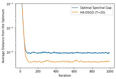
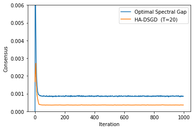
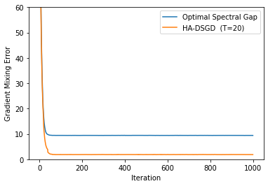
Figure 1: Comparison of HA-DSGD to D-SGD. (a) Average distance from the optimum, (b) consensus distance $\smash{\frac{1}{n}\big{\|}X-\overline{X}\big{\|}_{F}^{2}}$, and (c) gradient mixing error $\smash{\big{\|}\partial F({X},\xi)W-\overline{\partial F}({X},\xi)\big{\|}_{F}^{2}}$ vs. the number of iterations for quadratic objectives. “Optimal Spectral Gap” denotes the DSGD algorithm with mixing matrix optimized for a spectral gap. We report an average over a window of 5 iterations of corresponding quantity on each plot.

Sketching for Gram Matrix Estimation.

The original GME-exact formulation requires transmitting the entire gradients. We instead propose to calculate the Gram matrix using sketched gradients, for improved communication efficiency.

Let $A$ denote a random matrix with Gaussian entries and let $U$ be an arbitrary matrix. We observe that $\mathbb{E}(UA)^{\top}UA=\mathbb{E}U^{\top}A^{\top}AU=U^{\top}U$. Therefore, the above projection operation preserves the inner products in expectation. The approximation error of the above scheme can be bounded using the following extension of the Johnson–Lindenstrauss lemma, whose proof can be found in the appendix:

Proposition 3.

Let $\{\mathbf{u}_{1},\cdots,\mathbf{u}_{m}\}\in\mathbb{R}^{d}$. Assume that the entries in $A\subset\mathbb{R}^{k\times d}$ are sampled independently from $\mathcal{N}(0,1)$. Then, for $k=\omega(\frac{log(\frac{m}{\delta})}{\varepsilon^{2}})$, with probability greater than $1-\delta$ , we have:

$$\left\lvert\tfrac{1}{k}\left\langle A\mathbf{u}_{i},A\mathbf{u}_{j}\right\rangle-\left\langle\mathbf{u}_{i},\mathbf{u}_{j}\right\rangle\right\rvert\leq\varepsilon\max_{i\in[m]}\left\lVert\mathbf{u}_{i}\right\rVert^{2}$$

for all $i,j\in[m]$.

See appendix for the proof. In our algorithm, the $\{\mathbf{u}_{1},\cdots,\mathbf{u}_{m}\}\in\mathbb{R}^{d}$ correspond to the gradients across nodes, and are compressed using a Gaussian matrix generated, independently at each period using shared seeds.

Use of local $X$.

In our practical implementation we solve GME problem for gradients computed at the parameters $X$ instead of $\overline{X}$ in GME-exact. We show that this leads to the minimization of the GME upto an additional term proportional to the consensus:

Proposition 4.

$\left\lVert\partial f(\overline{X})W-\overline{\partial f}(\overline{X})\right\rVert_{F}^{2}$
$~{}~{}\leq~{}~{}2\left\lVert\partial f(X)W-\overline{\partial f}(X)\right\rVert_{F}^{2}+2L^{2}\left\lVert X-\overline{X}\right\rVert_{F}^{2}$

We prove this proposition in the appendix. We also give an estimate of the decrease of consensus distance $\|X-\overline{X}\|_{F}^{2}$. Thus, the small right hand side ensures the small relative heterogeneity.

5.4 Discussion & Extensions

Optimizing Mixing of updates of arbitrary algorithms: Our approach can be generalized to arbitrary additive updates to the parameters of the form $\mathbf{x}_{i}^{(t+1)}=\mathbf{x}_{i}^{(t)}+\eta\mathbf{u}_{i}^{(t)}$. For example, replacing the gradients in the Algorithm 2 by the updates of the Adam algorithm (Kingma & Ba, 2015) results in the minimization of the mixing error involved in decentralized Adam updates. We empirically verify the effectiveness of such an algorithm for an NLP task as discussed in Section 6.2.

Optimizing Mixing of Parameters: An alternate way of simultaneously maximizing the consensus factor $p$ and the gradient mixing error is to directly optimize the mixing error of the parameters i.e. $\big{\|}(X^{(t)}-\overline{X}^{(t)})W\big{\|}_{F}^{2}$. Our theoretical analysis covers such a choice of mixing matrices as a special case that involves trying to obtain a mixing matrix having both small $(1-p)$ and the gradient mixing error. However, unlike the gradient mixing error that involves changes of the order $\eta^{2}$ as shown by Lemma 1, the distribution of the parameters across nodes can change rapidly due to the mixing. Moreover, we found both approaches to yield similar improvements in practice and focus on the gradient mixing error since it covers a wider range of design choices such as mixing within unbiased cliques.

Method	Ring (n=$16$)	Torus (n=$16$)	Social Network (n=$32$)
DSGD	$74.71\pm 2.24$	$76.13\pm 1.65$	$77.68\pm 1.42$
HA-DSGD	$78.21\pm 2.19$	$79.08\pm 2.07$	$79.54\pm 1.61$
HA-DSGD (momemtum, period=100)	$80.75\pm 1.84$	$82.22\pm 1.87$	$83.24\pm 1.15$
DSGD (momentum, Metropolis-Hastings)	$77.52\pm 2.78$	$80.45\pm 2.27$	$80.71\pm 1.93$
DSGD (momentum, Optimal Spectral Gap)	$79.06\pm 1.82$	$80.28\pm 2.12$	$80.91\pm 1.74$
$D^{2}$	$49.68\pm 3.19$	$51.37\pm 2.68$	$52.15\pm 2.43$

Table 1: Top-1 test accuracy on CIFAR10 under different topologies. The results in the table are averaged over three random seeds.

6 Experiments

For all our experiments, we use the CVXPY (Diamond & Boyd, 2016) convex optimization library to perform the constrained optimization defined in the section. In all our results, the period denotes the number of updates after which the mixing matrix is recomputed i.e. a period of $100$ implies that the communication of the compressed gradients and the computation of the mixing matrix occurs only for a $\frac{1}{100}$ fraction of the updates. We denote the number of nodes in the underlying topology by $n$. HA-DSGD refers to our proposed Alg. 2 with updates alternating between the weights obtained by the GME optimization and the Metropolis-Hastings weights, similarly as discussed in Section 4.2.

6.1 Quadratic Objectives

We first consider a simple setting of random quadratic objectives, with the objective for the $i_{th}$ client given by $f_{i}(\mathbf{x})=\left\lVert A_{i}\mathbf{x}+b_{i}\right\rVert^{2}_{2}$, where $\mathbf{x}$ denotes a $d$ dimensional parameter vector and both $A_{i}$ and $b_{i}$ contain entries sampled randomly from $\mathcal{N}(0,1)$ and fixed for each client. For our experiments, we set $d=10$. We further introduce stochasticity to the gradients by adding random Gaussian noise with variance $0.1$. We generate a random connected graph of $16$ nodes by randomly removing half of the edges from a complete graph, while ensuring that the connectivity is maintained. Figure 1 illustrates the improvements due to our approach across three metrics: the distance from the optimum, consensus error, as well as the gradient mixing error.

6.2 Deep Learning Benchmarks

We evaluate our approach on computer vision as well as natural language processing benchmarks. Following Yurochkin et al. (2019), for each setting, the heterogeneity across clients is governed by a Dirichlet distribution-based partitioning scheme with a parameter $\alpha$ quantifying the dissimilarity between the data distributions across nodes. We set $\alpha=0.1$ for all the experiments since it corresponds to a setting with high heterogeneity. We compare against the baseline DSGD with local momentum under mixing weights defined by the Metropolis-Hastings scheme as well as those obtained through the optimization of the spectral gap (Boyd et al., 2003). We use standard learning rate scaling and warmup schedules as described in (Goyal et al., 2018) for the computer vision tasks and use a constant learning rate with Adam optimizer (Kingma & Ba, 2015) for the NLP task. Further experimental details for all the settings are outlined in Appendix D.

Compression Dimension	Test Accuracy
1	$75.66$
100	$81.55$
1000	$81.97$

Table 2: Effect of the Compression Dimension on the top-1 test accuracy on the CIFAR dataset.

Method	Ring (n=$16$)	Torus (n=$16$)
DAdam	$87.14\pm 0.71$	$87.42\pm 0.65$
HA-DSGD(Adam)	$89.29\pm 0.48$	$89.73\pm 0.54$

Table 3: Top-1 test accuracy on the AGNews dataset under different topologies. The results in the table are averaged over three random seeds.

CIFAR10. We evaluate our approach on the CIFAR10 dataset (Krizhevsky, 2009) by training the Resnet20 model (He et al., 2015) with Evonorm (Liu et al., 2020) for 300 epochs for each model. Following Sec. 5.4, we consider the extension of our algorithm to the mixing of Nesterov momentum updates, denoted by HA-DSGD (momentum) in Table 1, and compare against the corresponding version of DSGD with momentum. We also compare against the $D^{2}$ algorithm (Tang et al., 2018) for completeness. The results show that our approach consistently outperforms the baselines across three topologies, ring ($n=16$), torus ($n=16$), as well as the topology defined by the Davis Southern Women dataset as available in the Networkx library (Hagberg et al., 2008). Since both the Metropolis-Hastings and the optimal spectral gap mixing schemes lead to similar results, we only compare against the Metropolis-Hastings schemes in the subsequent tasks.

Transformer on AG News. We evaluate the extension of our algorithm to the mixing of Adam (Kingma & Ba, 2015) updates on the NLP task of fine-tuning the distilbert-base-uncased model (Wolf et al., 2020) on the AGNews dataset (Zhang et al., 2015). Table 3 verifies the applicability of our approach to Adam updates.

Imagenet. To evaluate our approach on a large-scale dataset, we consider the task of training a Resnet18 model (He et al., 2015) with evonorm on the Imagenet dataset (Deng et al., 2009). We use a larger period of 1000 for the optimization of the mixing matrix to account for the larger number of steps per epoch. We train each model using Nesterov momentum for 90 epochs using a ring topology defined on $16$ nodes. Similar to other settings, our approach as shown in Table 4 outperforms DSGD, demonstrating its effectiveness under large period and dataset sizes.

6.3 Effect of the Compression Dimension

Proposition 3 predicts that a low approximation error in the entries of the Gram matrix can be achieved through compression with dimension independent of the number of parameters and logarithmic in the number of nodes. We empirically verify this for the CIFAR10 dataset using HA-DSGD with Nesterov momemtum and a period of $100$.

Method	Ring (n=$16$)
HA-DSGD(momentum, period=1000)	$55.14\pm 0.215$
DSGD (momentum)	$53.22\pm 0.25$

Table 4: Top-1 Test accuracy on the Imagenet dataset, The results in the table are averaged over three random seeds.

In Table 2, we observe that using a sketching dimension of $1$ leads to a significantly low performance while increasing the compression dimension to $1000$ leads to a marginal improvement in the test accuracy.

7 Conclusion and Future Work

In this work, we extended the analysis of DSGD to incorporate the interaction between the mixing matrix and the data heterogeneity, leading to a novel technique for dynamically adapting the mixing matrix throughout training. We focused on a general data-dependant mixing-based analysis of the DSGD algorithm with doubly-stochastic matrices for non-convex and convex-objectives. Future work could involve extending our technique to algorithms designed for specific settings such as EXTRA (Shi et al., 2015a) for convex non-stochastic cases, as well as approaches based on row-stochastic, column-stochastic matrices and time-varying topologies. On the theoretical side, promising directions include extending our analysis to the mixing of momentum.

Appendix A Proofs of Main Results

A.1 Preliminaries

We utilize the following set of standard useful inequalities:

Lemma 1.

Let $g$ be an $L$-smooth convex function. Then we have:

$$\left\lVert\nabla g(\mathbf{x})-\nabla g(\mathbf{y})\right\rVert_{2}^{2} \leq 2L\left(g(\mathbf{x})-g(\mathbf{y})-\left\langle\mathbf{x}-\mathbf{y},\nabla g(\mathbf{y})\right\rangle\right)\,, \forall\mathbf{x},\mathbf{y}\in\mathbb{R}^{d},$$ (12)

Lemma 2.

Let $Y\in\mathbb{R}^{d\times n}$ be an arbitrary matrix and $\overline{Y}$ the matrix with each column containing the columnwise mean of $Y$ i.e. $\overline{Y}=Y\frac{\bm{1}\bm{1}^{\top}}{n}$. Then we have:

$$\left\lVert Y-\overline{Y}\right\rVert_{F}^{2}=\left\lVert Y\right\rVert_{F}^{2}-\left\lVert\overline{Y}\right\rVert_{F}^{2}\leq\left\lVert Y\right\rVert_{F}^{2}.$$ (13)

Lemma 3.

For arbitrary set of $n$ vectors $\{\mathbf{a}_{i}\}_{i=1}^{n}$, $\mathbf{a}_{i}\in\mathbb{R}^{d}$

$$\left\lVert\sum_{i=1}^{n}\mathbf{a}_{i}\right\rVert^{2}\leq n\sum_{i=1}^{n}\left\lVert\mathbf{a}_{i}\right\rVert^{2}\,.$$ (14)

Lemma 4.

For given two vectors $\mathbf{a},\mathbf{b}\in\mathbb{R}^{d}$

$$\left\lVert\mathbf{a}+\mathbf{b}\right\rVert^{2}\leq(1+\alpha)\left\lVert\mathbf{a}\right\rVert^{2}+(1+\alpha^{-1})\left\lVert\mathbf{b}\right\rVert^{2},\,\, \forall\alpha>0\,.$$ (15)

This inequality also holds for the sum of two matrices $A,B\in\mathbb{R}^{n\times d}$ in Frobenius norm.

A.2 Recursion For Consensus

The recursion for consensus, analyzed in Lemmas 9 and 12 of Koloskova et al. (2020b) relies on the following inequalities:

$$n\Xi_{t} =\mathbb{E}{\left\lVert X^{(t)}-\overline{X}^{(t)}\right\rVert_{F}^{2}}=\mathbb{E}\left\lVert X^{(t)}-\overline{X}^{(t-1)}-\left(\overline{X}^{(t)}-\overline{X}^{(t-1)}\right)\right\rVert_{F}^{2}\leq\mathbb{E}\left\lVert X^{(t)}-\overline{X}^{(t-1)}\right\rVert_{F}^{2}$$

The above inequality, however, discards the fact that it is desirable for the update at each node to be close to the update to the mean. Our analysis below instead incorporates the effect of the mixing of the gradient through the following lemma:

Lemma 5.

The update to $X^{(t-1)}$ at the $t_{th}$ step of algorithms 1 and 2 with mixing matrix $W^{(t-1)}$ can be reformulated as:

$$X^{(t)}-\overline{X}^{(t)}=\left(X^{(t-1)}-\overline{X}^{(t-1)}\right)W^{(t-1)}-\eta_{t}\left(\partial F(X^{(t-1)},\xi^{(t-1)})-\overline{\partial F}(X^{(t-1)},\xi^{(t-1)})\right)W^{(t-1)}$$ (16)

Proof.

$$X^{(t)}-\overline{X}^{(t)}=(X^{(t-1)}-\eta_{t}\partial F(X^{(t-1)},\xi^{(t-1)}))(W^{(t-1)}-\frac{1}{n}\bm{1}\bm{1}^{\top})$$

$$=X^{(t-1)}W^{(t-1)}-\overline{X}^{(t-1)}-\eta_{t}\left(\partial F(X^{(t-1)},\xi^{(t-1)})W^{(t-1)}-\overline{\partial F}(X^{(t-1)},\xi^{(t-1)})\right)$$

$$=\left(X^{(t-1)}-\overline{X}^{(t-1)}\right)W^{(t-1)}-\eta_{t}\left(\partial F(X^{(t-1)},\xi^{(t-1)})-\overline{\partial F}(X^{(t-1)},\xi^{(t-1)})\right)W^{(t-1)}.$$

Where in the last step we used the identity $\frac{\bm{1}\bm{1}^{\top}}{n}W=\frac{\bm{1}\bm{1}^{\top}}{n}$, valid for any doubly stochastic matrix $W$, implying that $\overline{X}^{(t-1)}W^{(t-1)}=\overline{X}^{(t-1)}$ and $\overline{\partial F}(X^{(t-1)},\xi^{(t-1)})W^{(t-1)}=\overline{\partial F}(X^{(t-1)},\xi^{(t-1)})$. ∎

For the sake of generality and consistency with (Koloskova et al., 2020b), we prove our result under a generalization of the Assumption 5 on the gradient mixing error

Assumption 6 (Relative Heterogenity with Growth).

We assume that there exist constants $\zeta^{\prime}$ and $P^{\prime}$, such that $\forall X\in\mathbb{R}^{d\times n}$:

Assumption 5 corresponds to a special case of the above assumption with $P^{\prime}=0$.

We now prove the following consensus recursion:

Lemma 6.

Let $\Xi_{t}=\frac{1}{n}\mathbb{E}_{t}{\sum_{i=1}^{n}\left\lVert\mathbf{x}_{i}^{(t)}-\overline{\mathbf{x}}^{(t)}\right\rVert^{2}}$ denote the consensus distance at time $t$, and let $e_{t}=f(\overline{\mathbf{x}}^{(t)})-f(\mathbf{x}^{\star})$ for the convex case and $e_{t}=\left\lVert\nabla f(\overline{\mathbf{x}}^{(t)})\right\rVert_{2}^{2}$ for the non-convex case. Then:

$$\Xi_{t} \leq\left(1-\frac{p}{2}\right)\Xi_{t-1}+D\eta_{t-1}^{2}e_{t-1}+A\eta_{t-1}^{2}.$$ (17)

Where $D=36L(1-p)+4L\frac{8-7p}{p}$ for the convex case , $\frac{8-7p}{p}P^{\prime}$ for the nonconvex case and $A=\frac{8-7p}{p}({\zeta^{\prime}}^{2})+3(1-p)\sigma^{2}$ for the non-convex case and $\frac{16-14p}{p}({\zeta^{\prime}}^{2})+9(1-p)\sigma^{2}$ for the convex case.

Proof.

$$\mathbb{E}_{W\sim\mathcal{W}}\tfrac{1}{n}\big{\|}\partial f(\overline{X})W-\overline{\partial f}(\overline{X})\big{\|}^{2}\leq\zeta^{\prime 2}+P^{\prime}\left\lVert{\partial f}(\overline{X})\right\rVert^{2}\,.$$ (18)

Let $\Xi_{t}=\frac{1}{n}\mathbb{E}_{t}{\sum_{i=1}^{n}\left\lVert\mathbf{x}_{i}^{(t)}-\overline{\mathbf{x}}^{(t)}\right\rVert^{2}}$ denote the consensus distance at time $t$. We have, using Lemma 5:

$$n\Xi_{t} =\mathbb{E}{\left\lVert X^{(t)}-\overline{X}^{(t)}\right\rVert_{F}^{2}}$$

$$=\mathbb{E}\left\lVert\left(X^{(t-1)}-\overline{X}^{(t-1)}\right)W^{(t-1)}-\eta_{t}\left(\partial F(X^{(t-1)},\xi^{(t-1)})-\overline{\partial F}(X^{(t-1)},\xi^{(t-1)})\right)W^{(t-1)}\right\rVert_{F}^{2}$$

$$=\underbrace{\mathbb{E}\left\lVert\left(X^{(t-1)}-\overline{X}^{(t-1)}\right)W^{(t-1)}-\eta_{t}\left(\partial f(X^{(t-1)})-\overline{\partial f}(X^{(t-1)})\right)W^{(t-1)}\right\rVert_{F}^{2}}_{=:T_{1}}$$

$$+\underbrace{\eta_{t}^{2}\mathbb{E}\left\lVert\left(\partial F(X^{(t-1)},\xi^{(t-1)})-\overline{\partial F}(X^{(t-1)},\xi^{(t-1)})\right)W^{(t-1)}-\left(\partial f(X^{(t-1)})-\overline{\partial f}(X^{(t-1)})\right)W^{(t-1)}\right\rVert^{2}_{F}}_{=:T_{2}}$$

Where the last inequality follows from the fact that noise in the gradient is independent at each time step, and also from unbiased stochastic gradients $\mathbb{E}_{\xi^{(t-1)}}\partial F(X^{(t-1)},\xi^{(t-1)})=\partial f(X^{(t-1)})$. We first observe that, using assumption 4, we have:

$$\mathbb{E}\left\lVert\left(\partial F(X^{(t-1)},\xi^{(t-1)})-\overline{\partial F}(X^{(t-1)},\xi^{(t-1)})\right)W^{(t-1)}-\left(\partial f(X^{(t-1)})-\overline{\partial f}(X^{(t-1)})\right)W^{(t-1)}\right\rVert^{2}_{F}$$

$$\leq(1-p)\mathbb{E}\left\lVert\left(\partial F(X^{(t-1)},\xi^{(t-1)})-\overline{\partial F}(X^{(t-1)},\xi^{(t-1)})\right)-\left(\partial f(X^{(t-1)})-\overline{\partial f}(X^{(t-1)})\right)\right\rVert^{2}_{F}$$

Furthermore, using equation (2), we have:

$$\mathbb{E}\left\lVert\left(\partial F(X^{(t-1)},\xi^{(t-1)})-\overline{\partial F}(X^{(t-1)},\xi^{(t-1)})\right)-\left(\partial f(X^{(t-1)})-\overline{\partial f}(X^{(t-1)})\right)\right\rVert^{2}_{F}\leq\mathbb{E}\left\lVert\partial F(X^{(t-1)},\xi^{(t-1)})-\partial f(X^{(t-1)})\right\rVert^{2}_{F}$$

We then add and subtract the gradients at the mean point $\partial F(\overline{X}^{(t-1)},\xi^{(t-1)})$ and the corresponding mean $\partial F(\overline{X}^{(t-1)})$ to obtain:

$$\mathbb{E}\left\lVert\left(\partial F(X^{(t-1)},\xi^{(t-1)})-\partial f(X^{(t-1)})\right)\right\rVert^{2}_{F}$$

$$\stackrel{{\scriptstyle\text{Lemma}\ \ref{remark:norm_of_sum}}}{{\leq~{}}}3\left\lVert\partial F(X^{(t-1)},\xi^{(t-1)})-\partial F(\overline{X}^{(t-1)},\xi^{(t-1)})\right\rVert^{2}+3\mathbb{E}\left\lVert\partial f(X^{(t-1)})-\partial F(\overline{X}^{(t-1)}\right\rVert^{2}$$

$$+3\mathbb{E}\left\lVert\partial F(\overline{X}^{(t-1)},\xi^{(t-1)})-\partial F(\overline{X}^{(t-1)})\right\rVert^{2}_{F}$$

Using the $L$ smoothness of each node’s objective (Assumption 1), the first two terms can be bounded as follows:

$$\mathbb{E}\left\lVert\partial F(X^{(t-1)},\xi^{(t-1)})-\partial F(\overline{X}^{(t-1)},\xi^{(t-1)})\right\rVert^{2} \leq L^{2}\mathbb{E}\left\lVert X^{(t-1)}-\overline{X}^{(t-1)}\right\rVert_{F}^{2}$$

Similarly, we have:

$$\begin{split}\mathbb{E}\left\lVert\partial f(X^{(t-1)})-\partial F(\overline{X}^{(t-1)})\right\rVert^{2}&\leq L^{2}\mathbb{E}\left\lVert X^{(t-1)}-\overline{X}^{(t-1)}\right\rVert_{F}^{2}.\end{split}$$ (19)

Subsequently, we utilize the assumptions on stochasticity 3 to bound the third term.

We proceed separately for the Convex and non-convex cases:

Convex Case: We add and subtract $\partial F(X^{\star},\xi^{(j)})$ and the corresponding mean $\partial F(X^{\star})$ to obtain:

$$\begin{split}&\mathbb{E}\left\lVert\partial F(\overline{X}^{(t-1)},\xi^{(t-1)})-\partial F(\overline{X}^{(t-1)})\right\rVert^{2}_{F}\\ &=\mathbb{E}\left\lVert\left(\partial F(\overline{X}^{(t-1)},\xi^{(t-1)})-\partial F(X^{\star},\xi^{(j)})\right)-\left(\partial F(\overline{X}^{(t-1)}-\partial F(X^{\star})\right)+\left(\partial F(X^{\star},\xi^{(j)})-\partial F(X^{\star}))\right)\right\rVert^{2}_{F}\\ &\stackrel{{\scriptstyle\text{Lemma}\ \ref{remark:norm_of_sum}}}{{\leq~{}}}3\mathbb{E}\left\lVert\partial F(\overline{X}^{(t-1)},\xi^{(t-1)})-\partial F(X^{\star},\xi^{(j)})\right\rVert^{2}_{F}+3\left\lVert\partial F(\overline{X}^{(t-1)})-\partial F(X^{\star})\right\rVert+3\left\lVert\partial F(X^{\star},\xi^{(j)})-\partial F(X^{\star}))\right\rVert^{2}_{F}\\ &\stackrel{{\scriptstyle\text{Lemma}\ \ref{remark:lsmooth_norm}}}{{\leq}}3\cdot 2Ln(f(\mathbf{x})-f(\mathbf{x}^{\star}))+3\cdot 2Ln(f(\mathbf{x})-f(\mathbf{x}^{\star}))+3n\overline{\sigma}^{2}\\ &=12Ln(f(\mathbf{x})-f(\mathbf{x}^{\star}))+3n\overline{\sigma}^{2}\end{split}$$ (20)

Non-convex Case: We directly utilize the uniform bound on the stochasticity (assumption 3) to obtain:

$$\mathbb{E}\left\lVert\partial F(\overline{X}^{(t-1)},\xi^{(t-1)})-\partial F(\overline{X}^{(t-1)})\right\rVert^{2}_{F}\leq n\hat{\sigma}^{2}$$ (21)

The final bound on $T_{2}$ is therefore given by:

Convex case:

$$T_{2}\leq\eta_{t}^{2}6(1-p)L^{2}\mathbb{E}\left\lVert\left(X^{(t-1)}-\overline{X}^{(t-1)}\right)\right\rVert_{F}^{2}+36(1-p)\eta_{t}^{2}Ln(f(\mathbf{x}^{(t-1})-f(\mathbf{x}^{\star}))+9n(1-p)\eta_{t}^{2}\overline{\sigma}^{2}$$

Non-convex case:

$$T_{2}\leq 6(1-p)\eta_{t}^{2}L^{2}\mathbb{E}\left\lVert\left(X^{(t-1)}-\overline{X}^{(t-1)}\right)\right\rVert_{F}^{2}+3n(1-p)\eta_{t}^{2}\overline{\sigma}^{2}$$

We now bound $T_{1}$ as follows:

$$\mathbb{E}\left\lVert\left(X^{(t-1)}-\overline{X}^{(t-1)}\right)W^{(t-1)}-\eta_{t}\left(\partial f(X^{(t-1)})-\overline{\partial f}(X^{(t-1)})\right)W^{(t-1)}\right\rVert_{F}^{2}$$

$$=\mathbb{E}\biggl{\|}\left(X^{(t-1)}-\overline{X}^{(t-1)}\right)W^{(t-1)}-\eta_{t}\left(\partial F(\overline{X}^{(t-1)})-\overline{\partial F}(\overline{X}^{(t-1)})\right)W^{(t-1)}$$

$$- \eta_{t}\left(\left(\partial f(X^{(t-1)})-\partial F(\overline{X}^{(t-1)})\right)-\left(\overline{\partial f}(X^{(t-1)})-\overline{\partial F}(\overline{X}^{(t-1)})\right)\right)W^{(t-1)}\biggr{\|}_{F}^{2}$$

$$\stackrel{{\scriptstyle\text{Lemma}\ \ref{remark:norm_of_sum_of_two}}}{{\leq~{}}} (1+\beta_{1})\mathbb{E}\biggl{\|}\left(X^{(t-1)}-\overline{X}^{(t-1)}\right)W^{(t-1)}$$

$$- \eta_{t}\left(\left(\partial f(X^{(t-1)})-\partial F(\overline{X}^{(t-1)})\right)-\left(\overline{\partial f}(X^{(t-1)})-\overline{\partial F}(\overline{X}^{(t-1)})\right)\right)W^{(t-1)}\biggr{\|}_{F}^{2}$$

$$+(1+\beta_{1}^{-1})\mathbb{E}\left\lVert-\eta_{t}\left(\partial F(\overline{X}^{(t-1)})-\overline{\partial F}(\overline{X}^{(t-1)})\right)W^{(t-1)}\right\rVert_{F}^{2}$$

$$\stackrel{{\scriptstyle\text{Lemma}\ \ref{remark:norm_of_sum_of_two}\ ,Assumption\ \ref{a:p}}}{{\leq~{}}} (1-p)(1+\beta_{1})(1+\beta_{2})\mathbb{E}\left\lVert\left(X^{(t-1)}-\overline{X}^{(t-1)}\right)\right\rVert_{F}^{2}$$

$$+ \eta_{t}^{2}(1-p)(1+\beta_{1})(1+\beta_{2}^{-1})\mathbb{E}\biggl{\|}\left(\partial f(X^{(t-1)})-\partial F(\overline{X}^{(t-1)})\right)$$

$$-\left(\overline{\partial f}(X^{(t-1)})-\overline{\partial F}(\overline{X}^{(t-1)})\right)\biggr{\|}_{F}^{2}$$

$$+(1+\beta_{1}^{-1})\mathbb{E}\left\lVert\eta_{t}\left(\partial F(\overline{X}^{(t-1)})-\overline{\partial F}(\overline{X}^{(t-1)})\right)W^{(t-1)}\right\rVert_{F}^{2}$$

The second term can be bounded by utilizing Equation 19 and Equation 2 as follows:

$$\mathbb{E}\biggl{\|}\left(\partial f(X^{(t-1)})-\partial F(\overline{X}^{(t-1)})\right)-\left(\overline{\partial f}(X^{(t-1)})-\overline{\partial F}(\overline{X}^{(t-1)})\right)\biggr{\|}_{F}^{2} \stackrel{{\scriptstyle\text{Lemma}\ \ref{remark:matvar}}}{{\leq}}\mathbb{E}\biggl{\|}\left(\partial f(X^{(t-1)})-\partial F(\overline{X}^{(t-1)})\right)\biggr{\|}_{F}^{2}$$

$$\stackrel{{\scriptstyle\ref{eq:smooth_bound}}}{{\leq}}L^{2}\left\lVert X^{(t-1)}-\overline{X}^{(t-1)}\right\rVert_{F}^{2}.$$

Therefore, we obtain:

$$T_{1} \leq\left((1-p)(1+\beta_{1})(1+\beta_{2})+\eta^{2}_{t}(1-p)(1+\beta_{1})(1+\beta_{2}^{-1})L^{2}\right)\left\lVert X^{(t-1)}-\overline{X}^{(t-1)}\right\rVert_{F}^{2}$$

$$\qquad\qquad+(1+\beta_{1}^{-1})\eta_{t}^{2}\mathbb{E}\left\lVert\left(\partial F(\overline{X}^{(t-1)})-\overline{\partial F}(\overline{X}^{(t-1)})\right)W^{(t-1)}\right\rVert_{F}^{2}$$

Finally, incorporating the bound on $T_{2}$, we obtain:

Convex Case:

$$n\Xi_{t} \leq\left((1-p)(1+\beta_{1})(1+\beta_{2}^{-1})+\eta^{2}_{t}(1-p)(1+\beta_{1})(1+\beta_{2}^{-1})\right)\left\lVert X^{(t-1)}-\overline{X}^{(t-1)}\right\rVert_{F}^{2}$$

$$\qquad+(1+\beta_{1}^{-1})\eta_{t}^{2}\mathbb{E}\left\lVert\left(\partial F(\overline{X}^{(t-1)})-\overline{\partial F}(\overline{X}^{(t-1)})\right)W^{(t-1)}\right\rVert_{F}^{2}+6(1-p)L^{2}\mathbb{E}\left\lVert\left(X^{(t-1)}-\overline{X}^{(t-1)}\right)\right\rVert_{F}^{2}$$

$$\qquad+36(1-p)\eta_{t}^{2}Ln(f(\mathbf{x})-f(\mathbf{x}^{\star}))+9n(1-p)\eta_{t}^{2}\overline{\sigma}^{2}$$

Nonconvex Case:

$$n\Xi_{t} \leq\left((1-p)(1+\beta_{1})(1+\beta_{2}^{-1})+\eta^{2}_{t}(1-p)(1+\beta_{1})(1+\beta_{2}^{-1})\right)\left\lVert\left(X^{(t-1)}-\overline{X}^{(t-1)}\right)\right\rVert_{F}^{2}$$

$$\qquad+(1+\beta_{1}^{-1})\eta_{t}^{2}\mathbb{E}\left\lVert\left(\partial F(\overline{X}^{(t-1)})-\overline{\partial F}(\overline{X}^{(t-1)})\right)W^{(t-1)}\right\rVert_{F}^{2}+6(1-p)L^{2}\eta_{t}^{2}\mathbb{E}\left\lVert\left(X^{(t-1)}-\overline{X}^{(t-1)}\right)\right\rVert_{F}^{2}+3n(1-p)\eta_{t}^{2}\overline{\sigma}^{2}$$

We now choose $\beta_{1}$ such that $(1-p)(1+\beta_{1})=(1-\frac{7p}{8})$ i.e. $\beta_{1}=\frac{p}{8(1-p)}$ Subsequently, we choose $\beta_{2}$ such that $((1-\frac{7p}{8})(1+\beta_{2})=(1-\frac{3p}{4})$ i.e. $\beta_{2}=\frac{p}{8-7p}$. Then, assuming that the step size $\eta_{t}$ satisfies, $\eta_{t}^{2}\leq\frac{\frac{p}{4}}{(1-p)(1+\beta_{1})(1+\beta_{2}^{-1})L^{2}+6(1-p)L^{2}}=\frac{\frac{p}{4}}{\left((1-\frac{7p}{8})\frac{8-6p}{p}+6(1-p)\right)L^{2}}$, we obtain:

$$n\Xi_{t}\leq (1-\frac{3p}{4})\mathbb{E}\left\lVert\left(X^{(t-1)}-\overline{X}^{(t-1)}\right)\right\rVert_{F}^{2}+\frac{p}{4}\mathbb{E}\left\lVert\left(X^{(t-1)}-\overline{X}^{(t-1)}\right)\right\rVert_{F}^{2}$$

$$+(1+\beta_{1}^{-1})\eta_{t}^{2}\mathbb{E}\left\lVert\left(\partial F(\overline{X}^{(t-1)})-\overline{\partial F}(\overline{X}^{(t-1)}\right)W^{(t-1)}\right\rVert_{F}^{2}+6(1-p)L^{2}\eta_{t}^{2}\mathbb{E}\left\lVert\left(X^{(t-1)}-\overline{X}^{(t-1)}\right)\right\rVert_{F}^{2}+3n(1-p)\eta_{t}^{2}\overline{\sigma}^{2}$$

$$\leq(1-\frac{p}{2})\mathbb{E}\left\lVert\left(X^{(t-1)}-\overline{X}^{(t-1)}\right)\right\rVert_{F}^{2}$$

$$+\eta_{t}^{2}(1+\beta_{1}^{-1})\mathbb{E}\left\lVert\left(\partial F(\overline{X}^{(t-1)})-\overline{\partial F}(\overline{X}^{(t-1)})\right)W^{(t-1)}\right\rVert_{F}^{2}+3n(1-p)\eta_{t}^{2}\overline{\sigma}^{2}$$

Since $\frac{\frac{p}{4}}{\left((1-\frac{7p}{8})\frac{8-6p}{p}+6(1-p)\right)L^{2}}\geq\frac{p^{2}}{80L^{2}}$, we only require the step size to be $\mathcal{O}(\frac{p^{2}}{L^{2}})$, same as Koloskova et al. (2020b). Thus the consensus distance decreases linearly, along with an error dependent on the diffusion of the gradients across nodes. Finally, substituting the assumption 6 for the non-convex case, we obtain:

$$n\Xi_{t}\leq(1-\frac{p}{2})\mathbb{E}\left\lVert\left(X^{(t-1)}-\overline{X}^{(t-1)}\right)\right\rVert_{F}^{2}+\eta_{t}^{2}\frac{8-7p}{p}({\zeta^{\prime}}^{2}+P^{\prime}\left\lVert\overline{\partial F}(\overline{X})\right\rVert^{2})$$

$$=(1-\frac{p}{2})\mathbb{E}\left\lVert\left(X^{(t-1)}-\overline{X}^{(t-1)}\right)\right\rVert_{F}^{2}+\eta_{t}^{2}(1+\beta_{1}^{-1}){\zeta^{\prime}}^{2}+\eta_{t}^{2}\frac{8-7p}{p}(1-p)P^{\prime}\left\lVert\overline{\partial F}(\overline{X})\right\rVert^{2}+3n(1-p)\eta_{t}^{2}\sigma^{2}.$$

For the convex case, we first bound the gradient mixing error at $X$ in terms of that at $X^{*}$ as follows:

$$\mathbb{E}\left\lVert\left(\partial F(\overline{X}^{(t-1)})-\overline{\partial F}(\overline{X}^{(t-1)})\right)W^{(t-1)}\right\rVert_{F}^{2}$$

$$=\mathbb{E}\left\lVert\left(\partial F(\overline{X}^{(t-1)})-\partial F(X^{*})-(\overline{\partial F}(\overline{X}^{(t-1)})-\overline{\partial F}(X^{*}))\right)W^{(t-1)}+\left(\partial F(X^{*})-\overline{\partial F}(X^{*})\right)W^{(t-1)}\right\rVert_{F}^{2}$$

$$\stackrel{{\scriptstyle\text{Lemma}\ \ref{remark:norm_of_sum}}}{{\leq~{}}}2\mathbb{E}\left\lVert\left(\partial F(\overline{X}^{(t-1)})-\partial F(X^{*})-(\overline{\partial F}(\overline{X}^{(t-1)})-\overline{\partial F}(X^{*}))\right)W^{(t-1)}\right\rVert^{2}_{2}+2\mathbb{E}\left\lVert\left(\partial F(X^{*})-\overline{\partial F}(X^{*})\right)W^{(t-1)}\right\rVert_{F}^{2}$$

$$\stackrel{{\scriptstyle\text{Assumption}\ \ref{a:p}}}{{\leq~{}}}2(1-p)\mathbb{E}\left\lVert\partial F(\overline{X}^{(t-1)})-\partial F(X^{*})-(\overline{\partial F}(\overline{X}^{(t-1)})-\overline{\partial F}(X^{*}))\right\rVert^{2}_{2}+2\mathbb{E}\left\lVert\left(\partial F(X^{*})-\overline{\partial F}(X^{*})\right)W^{(t-1)}\right\rVert_{F}^{2}$$

$$\stackrel{{\scriptstyle\text{Lemma}\ \ref{remark:matvar}}}{{\leq~{}}}2(1-p)\mathbb{E}\left\lVert\partial F(\overline{X}^{(t-1)})-\partial F(X^{*})\right\rVert^{2}_{2}+2\mathbb{E}\left\lVert\left(\partial F(X^{*})-\overline{\partial F}(X^{*})\right)W^{(t-1)}\right\rVert_{F}^{2}$$

$$\leq 2(1-p)\mathbb{E}\left\lVert\partial F(\overline{X}^{(t-1)})-\partial F(X^{*})\right\rVert^{2}_{2}+2\mathbb{E}\left\lVert\left(\partial F(X^{*})-\overline{\partial F}(X^{*})\right)W^{(t-1)}\right\rVert_{F}^{2}$$

$$\leq 4(1-p)L\mathbb{E}\left(f(\overline{\mathbf{x}}^{(t-1)})-f(\mathbf{x}^{\star})\right)+2\mathbb{E}\left\lVert\left(\partial F(X^{*})-\overline{\partial F}(X^{*})\right)W^{(t-1)}\right\rVert_{F}^{2}.$$

Where in the last step, we used Equation 1. Therefore, we obtain:

$$n\Xi_{t} \leq(1-\frac{p}{2})\mathbb{E}\left\lVert\left(X^{(t-1)}-\overline{X}^{(t-1)}\right)\right\rVert_{F}^{2}$$

$$+4(1-p)\eta_{t}^{2}\frac{8-7p}{p}L\mathbb{E}\left(f(\overline{\mathbf{x}}^{(j)})-f(\mathbf{x}^{\star})\right)+2\eta_{t}^{2}(1+\beta_{1}^{-1})n\overline{\zeta}^{2}+36Ln(1-p)\eta_{t}^{2}(f(\mathbf{x})-f(\mathbf{x}*))+9n(1-p)\eta_{t}^{2}\overline{\sigma}^{2}$$

∎

A.3 Convergence Rate

We utilize the consensus recursion in Lemma 6 to bound an appropriately weighted sum of the consensus iterates as follows:

$$\sum_{t=0}^{T}w_{t}n\Xi_{t}\leq\sum_{t=1}^{T}w_{t}(1-\frac{p}{2})n\Xi_{t-1}+\sum_{t=1}^{T}w_{t}\eta_{t-1}^{2}De_{t-1}+\sum_{t=1}^{T}w_{t}\eta_{t-1}^{2}A$$

Recursively substituting $n\Xi_{t-1}$ for $t$ in $[1,\cdots,T]$, we then obtain:

$$\sum_{t=0}^{T}w_{t}n\Xi_{t} \leq\sum_{t=1}^{T}\sum_{j=0}^{t-1}w_{t}\eta_{j}^{2}(1-\frac{p}{2})^{t-j-1}(De_{j}+A)$$

$$=\sum_{t=1}^{T}\sum_{j=0}^{t-1}w_{t}\eta_{j}^{2}(1-\frac{p}{2})^{t-j-1}(De_{j}+A)$$

$$=\sum_{j=0}^{T-1}\sum_{t=j+1}^{T}\eta_{j}^{2}w_{t}(1-\frac{p}{2})^{t-j-1}(De_{j}+A)$$

$$\leq\sum_{j=0}^{T}\sum_{t=j+1}^{\infty}\eta_{j}^{2}w_{t}(1-\frac{p}{2})^{t-j-1}(De_{t-1}+A)$$

$$\leq\sum_{j=0}^{T}\eta_{j}^{2}\frac{2}{p}w_{j}(De_{j}+A)\ .$$

Where in the last step we used $w_{t}\leq w_{j}$ for $j\geq t$

We thus obtain an Equation having the same form as Equation 18 of (Koloskova et al., 2020b) :

$$B\cdot\sum_{t=0}^{T}w_{t}\Xi_{t}\ \leq\ \frac{b}{2}\cdot\sum_{t=0}^{T}w_{t}e_{t}+AB\frac{2}{p}\cdot\sum_{t=0}^{T}w_{t}\eta_{t}^{2}\,,$$ (22)

where $\eta$ satisfies $\eta\leq\sqrt{\frac{pbD}{2B}}$ and the factor $B$ is as defined in (Koloskova et al., 2020a) for the different cases.

The rest of the proof involves utilizing the descent lemma in (Koloskova et al., 2020b) and choosing the appropriate step size following exactly the use of Equation 18 in (Koloskova et al., 2020b). Finally, setting $P^{\prime}=0$ leads to the convergence rates provided in Theorem 1.

A.4 Proof of Proposition 1

We first note that

$$\overline{X}^{(t+H)}-\overline{X}^{(t)}=\sum_{i=0}^{H-1}-\eta_{t+i}\partial f(X^{(t+i)})$$ (23)

We further have:

$$\left\lVert\left(\partial f\left(\overline{X}^{(t+H)}\right)-\overline{\partial f}\left(\overline{X}^{(t+H)}\right)\right)W^{(t)}\right\rVert^{2}_{F} \stackrel{{\scriptstyle\text{Lemma}\ \ref{remark:norm_of_sum}}}{{\leq~{}}}2\left\lVert\left(\partial f\left(\overline{X}^{(t)}\right)-\overline{\partial f}\left(\overline{X}^{(t)}\right)\right)W^{(t)}\right\rVert^{2}_{F}$$

$$+2\left\lVert\left(\partial f\left(\overline{X}^{(t+H)}\right)-\overline{\partial f}\left(\overline{X}^{(t+H)}\right)-\left(\partial f\left(\overline{X}^{(t)}\right)-\overline{\partial f}\left(\overline{X}^{(t)}\right)\right)\right)W^{(t)}\right\rVert^{2}_{F}$$

Applying Lemma 2 to the second term in the RHS yields:

$$\left\lVert\left(\partial f\left(\overline{X}^{(t+H)}\right)-\overline{\partial f}\left(\overline{X}^{(t+H)}\right)\right)W^{(t)}\right\rVert^{2}_{F} \stackrel{{\scriptstyle Lemma\ref{remark:matvar}}}{{\leq~{}}}2\left\lVert\left(\partial f\left(\overline{X}^{(t)}\right)-\overline{\partial f}\left(\overline{X}^{(t)}\right)\right)W^{(t)}\right\rVert^{2}_{F}+2\left\lVert\left(\partial f\left(\overline{X}^{(t+H)}\right)-\partial f\left(\overline{X}^{(t)}\right)\right)W^{(t)}\right\rVert^{2}_{F}$$

Finally, using Equation 23 and the $L$-smoothness of the objectives (Assumption 1), we obtain:

$$\left\lVert\left(\partial f\left(\overline{X}^{(t+H)}\right)-\overline{\partial f}\left(\overline{X}^{(t+H)}\right)\right)W^{(t)}\right\rVert^{2}_{F} \leq 2\left\lVert\left(\partial f\left(\overline{X}^{(t)}\right)-\overline{\partial f}\left(\overline{X}^{(t)}\right)\right)W^{(t)}\right\rVert^{2}_{F}+2L^{2}\left\lVert\overline{X}^{(t+H)}-\overline{X}^{(t)}\right\rVert^{2}$$

$$\leq 2\left\lVert\left(\partial f\left(\overline{X}^{(t)}\right)-\overline{\partial f}\left(\overline{X}^{(t)}\right)\right)W^{(t)}\right\rVert^{2}_{F}+2H\sum_{i=0}^{H-1}\eta_{t}^{2}L^{2}\left\lVert\partial f(X^{(t+i)})\right\rVert^{2}_{F}\$$

A.5 Proof of Proposition 4

We start by adding and subtracting the corresponding gradients at the mean parameters $X$:

$$\left\lVert\left(\partial f(\overline{X})-\overline{\partial f}(\overline{X})\right)W\right\rVert_{F}^{2} =\left\lVert\left(\partial f(\overline{X})-\partial f(X)-\left(\overline{\partial f}(\overline{X})-\overline{\partial f}(X)\right)\right)W+\left(\partial f(X)-\overline{\partial f}(X)\right)W\right\rVert_{F}^{2}$$

$$\stackrel{{\scriptstyle\text{Lemma}\ \ref{remark:norm_of_sum}}}{{\leq~{}}}\left\lVert\left(\partial f(\overline{X})-\partial f(X)-\left(\overline{\partial f}(\overline{X})-\overline{\partial f}(X)\right)\right)\right\rVert_{F}^{2}+2\left\lVert\left(\partial f(X)-\overline{\partial f}(X)\right)W\right\rVert_{F}^{2}$$

$$\stackrel{{\scriptstyle\text{Lemma}\ \ref{remark:matvar}}}{{\leq~{}}}2\left\lVert\left(\partial f(\overline{X})-\partial f(X)\right)\right\rVert_{F}^{2}+2\left\lVert\left(\partial f(X)-\overline{\partial f}(X)\right)W\right\rVert_{F}^{2}$$

$$\stackrel{{\scriptstyle\text{Lemma}\ \ref{a:lsmooth}}}{{\leq~{}}}L^{2}\left\lVert X-\overline{X}\right\rVert_{F}^{2}+2\left\lVert\left(\partial f(X)-\overline{\partial f}(X)\right)W\right\rVert_{F}^{2},$$

A.6 Spectral Norm of Doubly Stochastic Matrices with Non-negative Entries

Proposition 5.

Let $W\in\mathbb{R}^{n\times n}$ be possibly asymmetric doubly stochastic matrix with non-negative entries. Then the spectral norm $\left\lVert W\right\rVert_{2}$ is bounded by $1$.

Proof.

We note that $W^{T}W$ is itself a symmetric doubly-stochastic matrix and therefore has an eigenvector $\frac{1}{\sqrt{n}}\bm{1}$ with eigenvalue $1$. Perron-Frobenius theorem then implies that the largest eigenvalue of $(W^{(t)})^{\top}W^{(t)}$ is bounded by $1$, completing the proof. ∎

A.7 Proof of Proposition 2

The proof proceeds by introducing the stochastic gradients into the LHS as follows:

$$\mathbb{E}\left[\left\lVert\left(\partial f(\overline{X})-\overline{\partial f}(\overline{X})\right)W^{*}(\xi)\right\rVert_{F}^{2}\right]=\mathbb{E}\left[\left\lVert\left(\partial f(\overline{X})-\overline{\partial f}(\overline{X})-\left(\partial f(\overline{X},\xi)-\overline{\partial f}(\overline{X},\xi)\right)+\left(\partial f(\overline{X},\xi)-\overline{\partial f}(\overline{X},\xi)\right)\right)W^{*}(\xi)\right\rVert_{F}^{2}\right]$$

$$\stackrel{{\scriptstyle\text{Lemma}\ \ref{remark:norm_of_sum}}}{{\leq~{}}}2\mathbb{E}\left[\left\lVert\left(\partial f(\overline{X},\xi)-\overline{\partial f}(\overline{X},\xi)\right)W^{*}(\xi)\right\rVert_{F}^{2}\right]+2\mathbb{E}\left[\left\lVert\left(\partial f(\overline{X})-\overline{\partial f}(\overline{X})-\left(\partial f(\overline{X},\xi)-\overline{\partial f}(\overline{X},\xi)\right)\right)W^{*}(\xi)\right\rVert^{2}_{2}\right]$$

$$\stackrel{{\scriptstyle\text{Lemma}\ \ref{remark:matvar}}}{{\leq~{}}}2\mathbb{E}\left[\left\lVert\left(\partial f(\overline{X},\xi)-\overline{\partial f}(\overline{X},\xi)\right)W^{*}(\xi)\right\rVert_{F}^{2}\right]+2\mathbb{E}\left[\left\lVert\left(\partial f(\overline{X})-\partial f(\overline{X},\xi)\right)W^{*}(\xi)\right\rVert^{2}_{2}\right].$$

Since $W^{*}(\xi)$ is doubly-stochastic, using Proposition 5, we obtain a bound on the spectral norm $\left\lVert W^{(*)}\right\rVert_{2}\leq 1$. Combining the bound on the spectral norm with the assumption on the variance yields:

$$\mathbb{E}\left[\left\lVert\left(\partial f(\overline{X})-\overline{\partial f}(\overline{X})\right)W^{*}(\xi)\right\rVert_{F}^{2}\right] \leq 2\mathbb{E}\left[\left\lVert\left(\partial f(\overline{X},\xi)-\overline{\partial f}(\overline{X},\xi)\right)W^{*}(\xi)\right\rVert_{F}^{2}\right]+2\mathbb{E}\left[\left\lVert\left(\partial f(\overline{X})-\partial f(\overline{X},\xi)\right)\right\rVert^{2}_{2}\right]$$

$$\leq 2\mathbb{E}\left[\left\lVert\left(\partial f(\overline{X},\xi)-\overline{\partial f}(\overline{X},\xi)\right)W^{*}(\xi)\right\rVert_{F}^{2}\right]+2\overline{\sigma^{2}}$$

A.8 Proof of Proposition 3

We utilize the following compression bound, that arises as a consequence of the concentration of $\chi^{2}$ random variables, as often utilized in the proof of the Johnson–Lindenstrauss lemma (Boucheron et al., 2013):

Lemma 7.

Let $\{\mathbf{u}_{1},\cdots,\mathbf{u}_{m}\}\in\mathbb{R}^{d}$. Assume that the entries in $A\subset\mathbb{R}^{k\times d}$ are sampled independently from $\mathcal{N}(0,1)$. Then, for $k\geq 100(\frac{log(\frac{m}{\delta})}{\varepsilon^{2}})$, with probability greater than $1-\delta$ , we have,$\forall i,j\in[m]$:

$$(1-\varepsilon)\left\lVert\mathbf{u}_{i}-\mathbf{u}_{j}\right\rVert^{2}\leq\frac{1}{k}\left\lVert A\mathbf{u}_{i}-A\mathbf{u}_{j}\right\rVert^{2}\leq(1+\varepsilon)\left\lVert\mathbf{u}_{i}-\mathbf{u}_{j}\right\rVert^{2}$$ (24)

Slightly weaker bounds can be obtained in more general settings such as that of sub-Gaussian random variables but we restrict to the Gaussian case in the theory as well as implementations of our algorithm.

Now, adding $\{-\mathbf{u}_{1},\cdots,-\mathbf{u}_{m}\}$ to the set of points and applying Lemma 7 yields, $\forall i,j\in[m]$:

$$\ (1-\varepsilon)\left\lVert\mathbf{u}_{i}-\mathbf{u}_{j}\right\rVert^{2}\leq\left\lVert A\mathbf{u}_{i}\pm A\mathbf{u}_{j}\right\rVert^{2}\leq(1+\varepsilon)\left\lVert\mathbf{u}_{i}-\mathbf{u}_{j}\right\rVert^{2}$$ (25)

Therefore, we bound the inner product as follows:

$$\frac{1}{k}\left\langle A\mathbf{u}_{i},A\mathbf{u}_{j}\right\rangle =\frac{1}{4k}\left(\left\lVert A\mathbf{u}_{i}+A\mathbf{u}_{j}\right\rVert^{2}-\left\lVert A\mathbf{u}_{i}-A\mathbf{u}_{j}\right\rVert^{2}\right)\leq\frac{1}{4}\left((1+\varepsilon)\left\lVert\mathbf{u}_{i}+\mathbf{u}_{j}\right\rVert^{2}-(1-\varepsilon)\left\lVert\mathbf{u}_{i}-\mathbf{u}_{j}\right\rVert^{2}\right)$$

$$\leq\left\langle\mathbf{u}_{i},\mathbf{u}_{j}\right\rangle+\frac{1}{2}\varepsilon\left(\left\lVert\mathbf{u}_{i}+\mathbf{u}_{j}\right\rVert^{2}+\left\lVert\mathbf{u}_{i}-\mathbf{u}_{j}\right\rVert^{2}\right)\leq\left\langle\mathbf{u}_{i},\mathbf{u}_{j}\right\rangle+\varepsilon\max_{i}\left\lVert\mathbf{u}_{i}\right\rVert^{2}$$

Similarly, we obtain the lower bound:

$$\left\langle\mathbf{u}_{i},\mathbf{u}_{j}\right\rangle-\varepsilon\max_{i}\left\lVert\mathbf{u}_{i}\right\rVert^{2}\leq\frac{1}{k}\left\langle A\mathbf{u}_{i},A\mathbf{u}_{j}\right\rangle$$

Appendix B Using different matrices for Parameter and Gradient Mixing

An additional advantage of our analysis is that it decouples the effect of parameter and gradient mixing. This allows our analysis to be extended to the case of use of different mixing matrices $W_{p}$ and $W_{g}$ for mixing the parameters and gradients at each step respectively. Concretely, we consider the following algorithm:

Algorithm 4 Decentralized SGD with decoupled mixing

0:  $X^{(0)}$, stepsizes $\{\eta_{t}\}_{t=0}^{T-1}$, number of iterations $T$, mixing matrix distributions $\mathcal{W}_{p}^{(t)},\mathcal{W}_{g}^{(t)}$, $t\in[0,T]$

1:  for $t$ in $0\dots T$ do in parallel on all workers

2:     $G^{(t)}=\partial F(X^{(t)},\xi^{(t)})$ $\triangleright$ stochastic gradients

3:     $W_{p}^{(t)}\sim\mathcal{W}_{p}^{(t)},W_{g}^{(t)}\sim\mathcal{W}_{g}^{(t)}$ $\triangleright$ sample mixing matrices

4:     $X^{(t+1)}=X^{(t)}W_{p}^{(t)}-\eta_{t}G^{(t)}W_{g}^{(t)}$ $\triangleright$ update & mixing

5:  end parallel for

We now show that the above algorithm leads to convergence rates having the same dependence on $p$ and $\zeta^{\prime}$ as Theorem 1 but with these parameters defined as above in terms of $\mathcal{W}_{u}^{(t)}$ and $\mathcal{W}_{g}^{(t)}$. For instance, for the Non-convex case, we obtain that $\frac{1}{T+1}\sum_{t=0}^{T}\mathbb{E}\left\lVert\nabla f(\overline{\mathbf{x}}^{(t)})\right\rVert_{2}^{2}\leq\varepsilon$ after

$$\mathcal{O}\left(\frac{\sigma^{2}}{n\varepsilon^{2}}+\frac{\zeta^{\prime}+\sigma\sqrt{p}}{p\varepsilon^{3/2}}+\frac{1}{p\varepsilon}\right)\cdot LF_{0}$$

iterations. Analogously, we obtain the corresponding convergence rates for the convex case with $\zeta_{\star}^{\prime}$ defined at the optimum i.e. $\mathbb{E}_{W_{g}\sim\mathcal{W}_{g}^{(t)}}\tfrac{1}{n}\big{\|}\partial f(X_{\star})W_{g}-\overline{\partial f}(X_{\star})\big{\|}^{2}\leq\zeta^{\prime 2}\,$. Similar to Lemma 5, the update can then be expressed as

$$X^{(t)}-\overline{X}^{(t)}=\left(X^{(t-1)}-\overline{X}^{(t-1)}\right)W_{p}^{(t-1)}-\eta_{t}\left(\partial F(X^{(t-1)},\xi^{(t-1)})-\overline{\partial F}(X^{(t-1)},\xi^{(t-1)})\right)W_{g}$$ (26)

Subsequently, analogous to the proof of Theorem 1, we obtain the following decomposition of the consensus iterates:

$$n\Xi_{t} =\underbrace{\mathbb{E}\left\lVert\left(X^{(t-1)}-\overline{X}^{(t-1)}\right)W_{u}^{(t-1)}-\eta_{t}\left(\partial f(X^{(t-1)})-\overline{\partial f}(X^{(t-1)})\right)W_{g}^{(t-1)}\right\rVert_{F}^{2}}_{=:T_{1}}$$

$$+\underbrace{\eta_{t}^{2}\mathbb{E}\left\lVert\left(\left(\partial F(X^{(t-1)},\xi^{(t-1)})-\overline{\partial F}(X^{(t-1)},\xi^{(t-1)})\right)-\left(\partial f(X^{(t-1)})-\overline{\partial f}(X^{(t-1)})\right)\right)W_{g}^{(t-1)}\right\rVert^{2}_{F}}_{=:T_{2}}$$

Now, for $p$ and $\zeta^{\prime}$ satisfying:

$$\mathbb{E}_{W_{u}\sim\mathcal{W}_{u}^{(t)}}\big{\|}XW_{u}-\overline{X}\big{\|}_{F}^{2}\leq(1-p)\big{\|}X-\overline{X}\big{\|}_{F}^{2}\,,$$ (27)

and,

$$\mathbb{E}_{W_{g}\sim\mathcal{W}_{g}^{(t)}}\tfrac{1}{n}\big{\|}\partial f(X)W_{g}-\overline{\partial f}(X)\big{\|}^{2}\leq\zeta^{\prime 2}\,,$$ (28)

we obtain the analogous consensus recursion:

$$\Xi_{t} \leq\left(1-\frac{p}{2}\right)\Xi_{t-1}+D\eta_{t-1}^{2}e_{t-1}+A\eta_{t-1}^{2}.,$$ (29)

where $D=36L+4L\frac{8-7p}{p}$ for the convex case , $\frac{8-7p}{p}P^{\prime}$ for the nonconvex case and $A=\frac{8-7p}{p}({\zeta^{\prime}}^{2})+3\sigma^{2}$ for the non-convex case and $\frac{16-14p}{p}({\zeta^{\prime}}^{2})+9\sigma^{2}$ for the convex case.

D-cliques (Bellet et al., 2021): Suppose that the graph can be divided into $K$ cliques, such that the mean gradient for each clique equals the mean across the entire graph. Let the nodes be numbered such that the $n_{k}$ nodes belonging to the $k_{th}$ clique succeed the $n_{k-1}$ nodes belonging to the ${(k-1)}_{th}$ clique. Then, we observe that utilizing a block matrix of the type

$$\left(\begin{matrix}\frac{1}{n_{1}}\bm{1}\bm{1}^{\top}&\mathbf{0}&\cdots&\mathbf{0}\\ \mathbf{0}&\frac{1}{n_{2}}\bm{1}\bm{1}^{\top}&\cdots&\mathbf{0}\\ \vdots&&&\vdots\\ \mathbf{0}&\mathbf{0}&\cdots&\frac{1}{n_{K}}\bm{1}\bm{1}^{\top}\end{matrix}\right)$$

leads to zero Gradient Mixing Error. This corresponds to the proposed algorithm in D-cliques (Bellet et al., 2021) where $W_{g}^{(t)}$ is set to a matrix performing uniform averaging within each clique, while $W_{u}^{(t)}$ utilizes all the edges for mixing. For unbiased cliques, we obtain $\zeta^{\prime}=0$. Therefore, our analysis above provides an explanation for the improvements achieved by decoupled parameter mixing and clique-averaging (Bellet et al., 2021) under the presence of unbiased cliques. We further note that, unlike the algorithm presented in (Bellet et al., 2021), our algorithm HA-DSGD with random sampling of mixing matrices does not involve the additional communication overhead for separately mixing the gradients at each time-step.

Appendix C Mixing Error under Permutations

We now demonstrate how the “Gradient Mixing Error” can be used to guide the choice of the arrangement of a given set of nodes over a graph. Given a set of nodes having fixed data distributions, the parameters controlling the Gradient Mixing Error (GME) is controlled by the choice of mixing weights as well as the graph topology. To illustrate the effects of the choice of topology on the convergence rates, we consider a toy setup of 4 nodes, having data distributions defined by quadratic objectives as in Section 6.1.

(a) Red plots denote HADSGD while the blue plots denote mixing using the matrix corresponding to the optimal spectral gap.

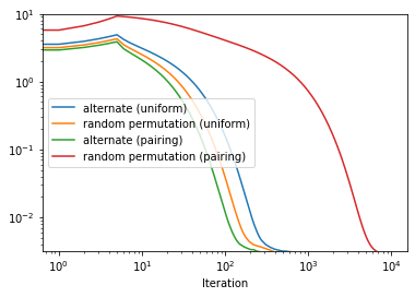
(b) The colors denote combinations of different permutations and mixing matrices.

Figure 2: Comparison of the distance from optimum vs number of iterations for different permutations of the nodes for (a) A random connected graph with 4 nodes (b) two-class ring topology setting with 16 nodes

To further illustrate the benefits of selecting an appropriate permutation, we consider a setup of 16 nodes distributed on a ring topology with the data distributions of exactly half of the nodes belonging to each one of the following class of objectives:

$$f_{1}(\mathbf{x}) =\left\lVert A(\mathbf{x}-\bm{1})\right\rVert^{2}$$

$$f_{2}(\mathbf{x}) =\left\lVert A(\mathbf{x}+\bm{1})\right\rVert^{2},$$

where $A$ denotes a fixed matrix with entries from $\mathcal{N}(0,1)$. We simulate the noise in SGD, by adding random vectors $\xi^{(t)}\sim\mathcal{N}(0,0.001)$ to the gradient updates for each node We compare the performance of DSGD under the following two permutations and choices of the mixing matrices:

1. Heterogenous pairing: As illustrated in Figure 3, the nodes are ordered around the ring alternating between the data for objectives $f_{1}$ and $f_{2}$. Subsequently, every node is paired with exactly one of its neighbours such that the mixing steps involve averaging between the members of the pairs with equal weights of $0.5$.

2. Random permutation: The nodes are randomly distributed on the ring with the mixing matrix corresponding to the maximal spectral gap.

Figure 3: Different arrangements of data and mixing weights across a ring topology: (left) Heterogenous pairing between adjacent nodes having different data distributions, (right) Random permutation of nodes with uniform weights. The colors red and blue indicate two different classes of data distributions.

Appendix D Architectures and Hyperparameters

Table 5: Experimental settings for Cifar-10

Dataset	Cifar-10
Data augmentation	random horizontal flip and random $32\times 32$ cropping
Architecture	Resnet20 with evonorm
Training objective	cross entropy
Evaluation objective	top-1 accuracy
Number of workers	16, 32
Topology	Ring, Torus, Social Network
Gossip weights	Metropolis-Hastings (1/3 for ring)
Data distribution	Heterogeneous, not shuffled, according to Dirichlet sampling procedure from Lin et al. (2021)
Batch size	32 patches per worker
Momentum	0.9 (Nesterov)
Learning rate	0.1 for $\alpha=0.1$
LR decay	$/10$ at epoch 150 and 180
LR warmup	Step-wise linearly within 5 epochs, starting from 0
# Epochs	300
Weight decay	$10^{-4}$
Normalization scheme	no normalization layer
Repetitions	3, with varying seeds

Table 6: Experimental settings for finetuning distilBERT

Dataset	AG News
Data augmentation	none
Architecture	DistilBERT
Training objective	cross entropy
Evaluation objective	top-1 accuracy
Number of workers	16
Topology	ring
Gossip weights	Metropolis-Hastings (1/3 for ring)
Data distribution	Heterogeneous, not shuffled, according to Dirichlet sampling procedure from Lin et al. (2021)
Batch size	32 patches per worker
Adam $\beta_{1}$	0.9
Adam $\beta_{2}$	0.999
Adam $\varepsilon$	$10^{-8}$
Learning rate	1e-6
LR decay	constant learning rate
LR warmup	no warmup
# Epochs	10
Weight decay	$0$
Normalization layer	LayerNorm (Ba et al., 2016),
Repetitions	3, with varying seeds

Table 7: Experimental settings for ImageNet

Dataset	ImageNet
Data augmentation	random resized crop ($224\times 224$), random horizontal flip
Architecture	ResNet-20-EvoNorm (Liu et al., 2020; He et al., 2015)
Training objective	cross entropy
Evaluation objective	top-1 accuracy
Number of workers	16
Topology	Ring
Gossip weights	Metropolis-Hastings (1/3 for ring)
Data distribution	Heterogeneous, not shuffled, according to Dirichlet sampling procedure from Lin et al. (2021)
Batch size	32 patches per worker
Momentum	0.9 (Nesterov)
Learning rate	$0.1\times\frac{32*16}{256}$)
LR decay	$/10$ at epoch $30,60,80$
LR warmup	Step-wise linearly within 5 epochs, starting from 0.1
# Epochs	90
Weight decay	$10^{-4}$
Normalization layer	EvoNorm (Liu et al., 2020)

References

• Alghunaim & Sayed (2020) Alghunaim, S. A. and Sayed, A. H. Linear convergence of primal–dual gradient methods and their performance in distributed optimization. Automatica, 117:109003, 2020. doi: https://doi.org/10.1016/j.automatica.2020.109003.
• Alghunaim & Yuan (2021) Alghunaim, S. A. and Yuan, K. A unified and refined convergence analysis for non-convex decentralized learning, 2021.
• Assran et al. (2019) Assran, M., Loizou, N., Ballas, N., and Rabbat, M. Stochastic gradient push for distributed deep learning. In Chaudhuri, K. and Salakhutdinov, R. (eds.), Proceedings of the 36th International Conference on Machine Learning, volume 97 of Proceedings of Machine Learning Research, pp.  344–353. PMLR, 09–15 Jun 2019.
• Ba et al. (2016) Ba, J. L., Kiros, J. R., and Hinton, G. E. Layer normalization, 2016.
• Bars et al. (2022) Bars, B. L., Bellet, A., Tommasi, M., and Kermarrec, A. Yes, topology matters in decentralized optimization: Refined convergence and topology learning under heterogeneous data, 2022.
• Bellet et al. (2021) Bellet, A., Kermarrec, A.-M., and Lavoie, E. D-cliques: Compensating noniidness in decentralized federated learning with topology, 2021.
• Boucheron et al. (2013) Boucheron, S., Lugosi, G., and Massart, P. Concentration inequalities. A nonasymptotic theory of independence. Oxford University Press, 2013.
• Boyd et al. (2003) Boyd, S., Diaconis, P., and Xiao, L. Fastest mixing markov chain on a graph. SIAM REVIEW, 46:667–689, 2003.
• Boyd et al. (2004) Boyd, S., Boyd, S. P., and Vandenberghe, L. Convex optimization. Cambridge university press, 2004.
• Dandi et al. (2021) Dandi, Y., Barba, L., and Jaggi, M. Implicit gradient alignment in distributed and federated learning, 2021.
• Deng et al. (2009) Deng, J., Dong, W., Socher, R., Li, L.-J., Li, K., and Fei-Fei, L. Imagenet: A large-scale hierarchical image database. In 2009 IEEE Conference on Computer Vision and Pattern Recognition, pp.  248–255, 2009. doi: 10.1109/CVPR.2009.5206848.
• Diamond & Boyd (2016) Diamond, S. and Boyd, S. CVXPY: A Python-embedded modeling language for convex optimization. Journal of Machine Learning Research, 17(83):1–5, 2016.
• Duchi et al. (2012) Duchi, J. C., Agarwal, A., and Wainwright, M. J. Dual averaging for distributed optimization: Convergence analysis and network scaling. IEEE Transactions on Automatic Control, 57(3):592–606, 2012. doi: 10.1109/TAC.2011.2161027.
• Frank & Wolfe (1956) Frank, M. and Wolfe, P. An algorithm for quadratic programming. Naval Research Logistics Quarterly, 3(1-2):95–110, 1956. doi: https://doi.org/10.1002/nav.3800030109.
• Goyal et al. (2018) Goyal, P., Dollár, P., Girshick, R., Noordhuis, P., Wesolowski, L., Kyrola, A., Tulloch, A., Jia, Y., and He, K. Accurate, large minibatch sgd: Training imagenet in 1 hour, 2018.
• Hagberg et al. (2008) Hagberg, A. A., Schult, D. A., and Swart, P. J. Exploring network structure, dynamics, and function using networkx. In Varoquaux, G., Vaught, T., and Millman, J. (eds.), Proceedings of the 7th Python in Science Conference, pp.  11 – 15, Pasadena, CA USA, 2008.
• He et al. (2015) He, K., Zhang, X., Ren, S., and Sun, J. Deep residual learning for image recognition, 2015.
• Hsieh et al. (2020) Hsieh, K., Phanishayee, A., Mutlu, O., and Gibbons, P. The non-iid data quagmire of decentralized machine learning. In International Conference on Machine Learning (ICML), pp. 4387–4398. PMLR, 2020.
• Jaggi (2013) Jaggi, M. Revisiting Frank-Wolfe: Projection-free sparse convex optimization. In Dasgupta, S. and McAllester, D. (eds.), Proceedings of the 30th International Conference on Machine Learning, volume 28 of Proceedings of Machine Learning Research, pp.  427–435, Atlanta, Georgia, USA, 17–19 Jun 2013. PMLR.
• Kairouz et al. (2021) Kairouz, P., McMahan, H. B., Avent, B., Bellet, A., Bennis, M., Bhagoji, A. N., Bonawitz, K., Charles, Z., Cormode, G., Cummings, R., D’Oliveira, R. G. L., Rouayheb, S. E., Evans, D., Gardner, J., Garrett, Z., Gascón, A., Ghazi, B., Gibbons, P. B., Gruteser, M., Harchaoui, Z., He, C., He, L., Huo, Z., Hutchinson, B., Hsu, J., Jaggi, M., Javidi, T., Joshi, G., Khodak, M., Konečný, J., Korolova, A., Koushanfar, F., Koyejo, S., Lepoint, T., Liu, Y., Mittal, P., Mohri, M., Nock, R., Özgür, A., Pagh, R., Raykova, M., Qi, H., Ramage, D., Raskar, R., Song, D., Song, W., Stich, S. U., Sun, Z., Suresh, A. T., Tramèr, F., Vepakomma, P., Wang, J., Xiong, L., Xu, Z., Yang, Q., Yu, F. X., Yu, H., and Zhao, S. Advances and open problems in federated learning. Foundations and Trends® in Machine Learning, 14(1–2):1–210, 2021.
• Karimireddy et al. (2020) Karimireddy, S. P., Kale, S., Mohri, M., Reddi, S. J., Stich, S. U., and Suresh, A. T. SCAFFOLD: Stochastic controlled averaging for on-device federated learning. In 37th International Conference on Machine Learning (ICML). PMLR, 2020.
• Kingma & Ba (2015) Kingma, D. P. and Ba, J. Adam: A method for stochastic optimization. In Bengio, Y. and LeCun, Y. (eds.), 3rd International Conference on Learning Representations, ICLR 2015, San Diego, CA, USA, May 7-9, 2015, Conference Track Proceedings, 2015.
• Koloskova et al. (2020a) Koloskova, A., Lin, T., Stich, S. U., and Jaggi, M. Decentralized deep learning with arbitrary communication compression. International Conference on Learning Representations (ICLR), 2020a.
• Koloskova et al. (2020b) Koloskova, A., Loizou, N., Boreiri, S., Jaggi, M., and Stich, S. A unified theory of decentralized SGD with changing topology and local updates. In III, H. D. and Singh, A. (eds.), Proceedings of the 37th International Conference on Machine Learning, volume 119 of Proceedings of Machine Learning Research, pp.  5381–5393. PMLR, 13–18 Jul 2020b.
• Koloskova et al. (2021) Koloskova, A., Lin, T., and Stich, S. U. An improved analysis of gradient tracking for decentralized machine learning. In NeurIPS, 2021.
• Kong et al. (2021) Kong, L., Lin, T., Koloskova, A., Jaggi, M., and Stich, S. U. Consensus control for decentralized deep learning. In Proceedings of the 38th International Conference on Machine Learning (ICML), volume 139, pp.  5686–5696. PMLR, 2021.
• Krizhevsky (2009) Krizhevsky, A. Learning multiple layers of features from tiny images. Technical report, 2009.
• Li et al. (2019) Li, X., Yang, W., Wang, S., and Zhang, Z. Communication efficient decentralized training with multiple local updates. arXiv preprint arXiv:1910.09126, 2019.
• Lian et al. (2017) Lian, X., Zhang, C., Zhang, H., Hsieh, C.-J., Zhang, W., and Liu, J. Can decentralized algorithms outperform centralized algorithms? a case study for decentralized parallel stochastic gradient descent. In Guyon, I., Luxburg, U. V., Bengio, S., Wallach, H., Fergus, R., Vishwanathan, S., and Garnett, R. (eds.), Advances in Neural Information Processing Systems, volume 30. Curran Associates, Inc., 2017.
• Lin et al. (2021) Lin, T., Karimireddy, S. P., Stich, S., and Jaggi, M. Quasi-global momentum: Accelerating decentralized deep learning on heterogeneous data. In Meila, M. and Zhang, T. (eds.), Proceedings of the 38th International Conference on Machine Learning, volume 139 of Proceedings of Machine Learning Research, pp.  6654–6665. PMLR, 18–24 Jul 2021.
• Liu et al. (2020) Liu, H., Brock, A., Simonyan, K., and Le, Q. Evolving normalization-activation layers. In Larochelle, H., Ranzato, M., Hadsell, R., Balcan, M. F., and Lin, H. (eds.), Advances in Neural Information Processing Systems, volume 33, pp.  13539–13550. Curran Associates, Inc., 2020.
• Long et al. (2018) Long, P., Fan, T., Liao, X., Liu, W., Zhang, H., and Pan, J. Towards optimally decentralized multi-robot collision avoidance via deep reinforcement learning. In 2018 IEEE International Conference on Robotics and Automation (ICRA), pp.  6252–6259. IEEE, 2018.
• Lorenzo & Scutari (2016) Lorenzo, P. D. and Scutari, G. NEXT: In-network nonconvex optimization. IEEE Transactions on Signal and Information Processing over Networks, 2(2):120–136, 2016. doi: 10.1109/TSIPN.2016.2524588.
• Lu et al. (2019) Lu, S., Zhang, X., Sun, H., and Hong, M. GNSD: A gradient-tracking based nonconvex stochastic algorithm for decentralized optimization. In 2019 IEEE Data Science Workshop (DSW), pp.  315–321. IEEE, 2019.
• Lu & De Sa (2021) Lu, Y. and De Sa, C. Optimal complexity in decentralized training. In Meila, M. and Zhang, T. (eds.), Proceedings of the 38th International Conference on Machine Learning, volume 139 of Proceedings of Machine Learning Research, pp.  7111–7123. PMLR, 18–24 Jul 2021.
• Mihaylov et al. (2009) Mihaylov, M., Tuyls, K., and Nowé, A. Decentralized learning in wireless sensor networks. In International Workshop on Adaptive and Learning Agents, pp.  60–73. Springer, 2009.
• Mitra et al. (2021) Mitra, A., Jaafar, R., Pappas, G., and Hassani, H. Linear convergence in federated learning: Tackling client heterogeneity and sparse gradients. Advances in Neural Information Processing Systems, 34, 2021.
• Nedic (2020) Nedic, A. Distributed gradient methods for convex machine learning problems in networks: Distributed optimization. IEEE Signal Processing Magazine, 37(3):92–101, 2020.
• Nedić & Ozdaglar (2009) Nedić, A. and Ozdaglar, A. Distributed subgradient methods for multi-agent optimization. IEEE Transactions on Automatic Control, 54(1):48–61, 2009.
• Nedic et al. (2016) Nedic, A., Olshevsky, A., and Shi, W. Achieving geometric convergence for distributed optimization over time-varying graphs. SIAM Journal on Optimization, 27, 07 2016. doi: 10.1137/16M1084316.
• Nedić et al. (2018) Nedić, A., Olshevsky, A., and Rabbat, M. G. Network topology and communication-computation tradeoffs in decentralized optimization. Proceedings of the IEEE, 106(5):953–976, 2018.
• Nedić et al. (2016) Nedić, A., Olshevsky, A., and Shi, W. Achieving geometric convergence for distributed optimization over time-varying graphs. SIAM Journal on Optimization, 27, 07 2016. doi: 10.1137/16M1084316.
• Neglia et al. (2020) Neglia, G., Xu, C., Towsley, D., and Calbi, G. Decentralized gradient methods: does topology matter? In Chiappa, S. and Calandra, R. (eds.), Proceedings of the Twenty Third International Conference on Artificial Intelligence and Statistics, volume 108 of Proceedings of Machine Learning Research, pp.  2348–2358. PMLR, 26–28 Aug 2020.
• Pu & Nedić (2020) Pu, S. and Nedić, A. Distributed stochastic gradient tracking methods. Mathematical Programming, pp.  1–49, 2020.
• Scaman et al. (2017) Scaman, K., Bach, F., Bubeck, S., Lee, Y. T., and Massoulié, L. Optimal algorithms for smooth and strongly convex distributed optimization in networks. In ICML - Proceedings of the 34th International Conference on Machine Learning, volume 70, pp.  3027–3036. PMLR, 2017.
• Shi et al. (2015a) Shi, W., Ling, Q., Wu, G., and Yin, W. Extra: An exact first-order algorithm for decentralized consensus optimization. SIAM Journal on Optimization, 25(2):944–966, 2015a. doi: 10.1137/14096668X.
• Shi et al. (2015b) Shi, W., Ling, Q., Wu, G., and Yin, W. EXTRA: An exact first-order algorithm for decentralized consensus optimization. SIAM Journal on Optimization, 25(2):944–966, 2015b.
• Tang et al. (2018) Tang, H., Lian, X., Yan, M., Zhang, C., and Liu, J. D2: Decentralized training over decentralized data. In Proceedings of the 35th International Conference on Machine Learning (ICML), volume 80, pp.  4848–4856. PMLR, 2018.
• Tsitsiklis (1984) Tsitsiklis, J. N. Problems in decentralized decision making and computation. PhD thesis, Massachusetts Institute of Technology, 1984.
• Vogels et al. (2021) Vogels, T., He, L., Koloskova, A., Lin, T., Karimireddy, S. P. R., Stich, S. U., and Jaggi, M. Relaysum for decentralized deep learning on heterogeneous data. In NeurIPS, 2021.
• Wang & Joshi (2018) Wang, J. and Joshi, G. Cooperative SGD: A unified framework for the design and analysis of communication-efficient SGD algorithms. arXiv preprint arXiv:1808.07576, 2018.
• Wang et al. (2019) Wang, J., Sahu, A. K., Yang, Z., Joshi, G., and Kar, S. MATCHA: Speeding up decentralized SGD via matching decomposition sampling. arXiv preprint arXiv:1905.09435, 2019.
• Wang et al. (2020a) Wang, J., Liu, Q., Liang, H., Joshi, G., and Poor, H. V. Tackling the objective inconsistency problem in heterogeneous federated optimization. In Advances in Neural Information Processing Systems, 2020a.
• Wang et al. (2021) Wang, J., Charles, Z., Xu, Z., Joshi, G., McMahan, H. B., y Arcas, B. A., Al-Shedivat, M., Andrew, G., Avestimehr, S., Daly, K., Data, D., Diggavi, S., Eichner, H., Gadhikar, A., Garrett, Z., Girgis, A. M., Hanzely, F., Hard, A., He, C., Horvath, S., Huo, Z., Ingerman, A., Jaggi, M., Javidi, T., Kairouz, P., Kale, S., Karimireddy, S. P., Konecny, J., Koyejo, S., Li, T., Liu, L., Mohri, M., Qi, H., Reddi, S. J., Richtarik, P., Singhal, K., Smith, V., Soltanolkotabi, M., Song, W., Suresh, A. T., Stich, S. U., Talwalkar, A., Wang, H., Woodworth, B., Wu, S., Yu, F. X., Yuan, H., Zaheer, M., Zhang, M., Zhang, T., Zheng, C., Zhu, C., and Zhu, W. A field guide to federated optimization. arXiv preprint arXiv:2107.06917, 2021.
• Wang et al. (2020b) Wang, X., Wang, C., Li, X., Leung, V. C., and Taleb, T. Federated deep reinforcement learning for internet of things with decentralized cooperative edge caching. IEEE Internet of Things Journal, 7(10):9441–9455, 2020b.
• Wei & Ozdaglar (2012) Wei, E. and Ozdaglar, A. Distributed alternating direction method of multipliers. In IEEE 51st IEEE Conference on Decision and Control (CDC), pp.  5445–5450, 2012.
• Wolf et al. (2020) Wolf, T., Debut, L., Sanh, V., Chaumond, J., Delangue, C., Moi, A., Cistac, P., Rault, T., Louf, R., Funtowicz, M., Davison, J., Shleifer, S., von Platen, P., Ma, C., Jernite, Y., Plu, J., Xu, C., Scao, T. L., Gugger, S., Drame, M., Lhoest, Q., and Rush, A. M. Huggingface’s transformers: State-of-the-art natural language processing, 2020.
• Woodworth et al. (2020) Woodworth, B. E., Patel, K. K., and Srebro, N. Minibatch vs local sgd for heterogeneous distributed learning. In NeurIPS, 2020.
• Xiao & Boyd (2004) Xiao, L. and Boyd, S. Fast linear iterations for distributed averaging. Systems & Control Letters, 53(1):65–78, 2004. ISSN 0167-6911. doi: https://doi.org/10.1016/j.sysconle.2004.02.022.
• Yuan & Alghunaim (2021) Yuan, K. and Alghunaim, S. A. Removing data heterogeneity influence enhances network topology dependence of decentralized sgd. arXiv preprint arXiv:2105.08023, 2021.
• Yuan et al. (2020) Yuan, K., Alghunaim, S. A., Ying, B., and Sayed, A. H. On the influence of bias-correction on distributed stochastic optimization. IEEE Transactions on Signal Processing, 68:4352–4367, 2020.
• Yuan et al. (2021) Yuan, K., Chen, Y., Huang, X., Zhang, Y., Pan, P., Xu, Y., and Yin, W. DecentLaM: Decentralized momentum SGD for large-batch deep training. In Proceedings of the IEEE/CVF International Conference on Computer Vision (ICCV), pp.  3029–3039, 2021.
• Yurochkin et al. (2019) Yurochkin, M., Agarwal, M., Ghosh, S., Greenewald, K., Hoang, N., and Khazaeni, Y. Bayesian nonparametric federated learning of neural networks. In Chaudhuri, K. and Salakhutdinov, R. (eds.), Proceedings of the 36th International Conference on Machine Learning, volume 97 of Proceedings of Machine Learning Research, pp.  7252–7261. PMLR, 09–15 Jun 2019.
• Zhang et al. (2015) Zhang, X., Zhao, J. J., and LeCun, Y. Character-level convolutional networks for text classification. In NIPS, 2015.