Random Manifold Sampling and Joint Sparse Regularization for Multi-label Feature Selection

Abstract

Multi-label learning is usually used to mine the correlation between features and labels, and feature selection can retain as much information as possible through a small number of features. $\ell_{2,1}$ regularization method can get sparse coefficient matrix, but it can not solve multicollinearity problem effectively. The model proposed in this paper can obtain the most relevant few features by solving the joint constrained optimization problems of $\ell_{2,1}$ and $\ell_{F}$ regularization. In manifold regularization, we implement random walk strategy based on joint information matrix, and get a highly robust neighborhood graph. In addition, we given the algorithm for solving the model and proved its convergence. Comparative experiments on real-world data sets show that the proposed method outperforms other methods.

1 Introduction

Different from multi-classification problem, an instance can have multiple labels at the same time in multi-label learning. As Zhihua Zhou and Zhiling Cai et al. studied in [34, 33, 4, 30], one input data will correspond to multiple outputs. It is facing some problems that need to be solved urgently, although multi-label learning has been very common in production and life. The first problem is that we often assume that labels are independent of each other when we make statistical inference, but in fact there is a strong correlation between different labels. The second problem is that multi-label data usually has very high feature dimension and label dimension, which leads to a sharp increase in learning cost and labeling cost. The third problem is that the number of samples on each label varies greatly. This problem is called label imbalance, which will lead to the failure of some labels, resulting in waste of information [25, 32].

When using the information of labels, previous studies often explore the high-order association between labels. Based on the association between labels, these methods can be roughly divided into three categories: (1) The first-order method, which always assumes that labels are independent of each other [6]. (2) Second-order method, which considers the correlation between labels [30]. (3) There are also high-order methods. Although they take more account of the interaction between labels, they are seldom used in practice because of their complexity [13].

If the dimension of data is too high, it will lead to ”dimension disaster” [7, 12]. Therefore, in order to avoid over-fitting in the process of model training, dimension reduction is usually carried out in the data preprocessing stage. Dimension reduction methods can be roughly divided into two categories: feature extraction and feature selection. The former is generally an unsupervised learning method, which obtains a few new features by combining, transforming and spectral decomposition of the original features. These new features greatly retain the information of the original features, but lost the meaning of the original features. For example, a small number of new features obtained by PCA after linear combination of original features are independent of each other, but the new features are not interpretable. Through eigenmap and neighborhood graph, LPP [9] preserves the local structure of data while reducing dimensions. Because of the poor interpretability of feature extraction methods, they are usually only used as intermediate results or visualization. Feature selection method directly selects a small number of high-value features from the original features by some means to achieve dimension reduction. Feature selection methods can generally be divided into three types: filter, wrapper and embedding. In the first two methods, the process of feature selection and model training is separate, so the model does not work very well on the task, and the computational overhead is relatively high. However, embedding method automatically completes feature selection in the process of training model, and its performance and computational overhead are usually superior to the former two. MCFS [3], RFS [21], LASSO [26] and other embedding methods generate sparse matrices for feature selection. They have been widely used in various tasks and have good performance.

The performance of global-based feature selection method on ultra high dimensional data is not always satisfactory, because the distribution of data in high-dimensional space is usually very complex. By paying attention to the local structure of data, manifold learning method [4, 31, 9] is superior to other methods. Nevertheless, manifold learning can’t avoid the problem of ”short circuit”, especially when the number of neighbors is not suitable.

When we consider the correlation between features, Hyunki Lim [17] builds a model to analyze the correlation between label pairs, and obtains a subset of features with low correlation. Arthur and Robert et al. proposed [10] ridge regression, which obtained a subset of variables with low correlation by punishing highly correlated variables. However, even when variables are highly correlated, they may get better results when working together than when working with several independent variables. The elastic net method [35] combines two or more features of a set of related features for consideration, so that the model has the ability to evaluate the collaborative work of features and avoids breaking the situation of multi-feature collaborative work.

Since the predicted value on labeled data should be greater than the predicted value on unlabeled data, we take the sum of squares of prediction errors as the loss function. In particular, when considering the neighborhood graph of manifold sampling, we use the joint information and implement the multi-step random walk strategy to construct the graph Laplacian matrix, so that the model can retain a highly robust local structure. On the basis of the above, we combine $\ell_{F}$ and $\ell_{2,1}$ regularization sum to obtain a highly sparse coefficient matrix, so as to realize feature selection.

The rest of this article is organized as follows: The related work is introduced in Section 2. In section 3, the model is established and the expression of the model is derived. In section 4, the algorithm for solving the model is given and the convergence of the algorithm is proved. In Section 5, data experiments are designed and the performance of the proposed algorithm on different data sets is demonstrated. Section 6 summarizes the work of this paper.

2 Related works

Predecessors have done a lot of research on how to make full use of label information. In ML-KNN, Zhihua Zhou et al. [34] predicted the label of new samples through the information of neighboring samples and posterior probability. Feng Kang and Wei Weng et al. make full use of the relevant information between labels through the label propagation algorithm [13, 30, 28], and get considerable results. When measuring the similarity between instances, Hamers and Kosub et al. [8, 14] suggest using Jaccard index. In their research, the author gives the probability basis of Jaccard index and shows its excellent performance. However, the above methods can not make full use of the sample information. For example, instance1:$x_{1}=(2,1,0,1),y_{1}=(0,1,1)$, instance2:$x_{2}=(2,1,1,1),y_{2}=(1,0,0)$, instance3:$x_{3}=(2,0,0,1),y_{3}=(0,0,1)$, instance1 is more similar to instance2 if we only consider features, but if we measure similarity by labels, instance1 and instance3 are more similar. Balasubramanian [2] called this phenomenon ”short circuit”, and based on this, put forward the concept of manifold learning. n order to avoid the ”short circuit” phenomenon, Roweis proposed LLE method in [23], which approximates the global nonlinear structure by local linear embedding. LPP method [9] firstly points out that high-dimensional data is projected into low-dimensional space, so as to realize dimension reduction by manifold learning method. A large number of studies have verified the effectiveness of LPP method. Quanmao Lu et al. [18] applied manifold embedding method to unsupervised learning dimension reduction and obtained excellent results. Miao Qi and Ronghua Shang et al. [24, 22] put forward the theory of projecting the loss function to the low-dimensional subspace and obtaining the optimal subspace by matrix factorization. However, these manifold methods are all based on KNN to construct neighborhood graphs, so the stability of local structure is easily affected by the number of neighbors. Laurensvan der Maaten and Xiaokai Wei et al. [19, 29] greatly improves the stability of manifold structure by adopting stochastic neighborhood embedding (SNE) method. Different from punishing the similarity between neighbors, Aiping Huang et al. [11] pay more attention to the linear combination of similarity vectors of samples, and they take the $\ell_{F}$-norm of similarity residual matrix as the loss function. All the above studies are unsupervised learning methods, so they can’t make effective use of label information when labels are given. We noticed that Ronghua Li and Fatemeh Vahedian et al. [15, 27, 16] studied the excellent properties of random walk in extracting the similarity of instances. Inspired by these studies, we introduce random walk strategy into the similarity sampling of manifold structure, which makes the model more robust.

RFS method [21] adds parameter regularization term to the multi-label learning model, which makes the coefficient matrix sparse and realizes feature selection. Similar to $\ell_{1}$-norm, $\ell_{2,1}$-norm does not consider the synergy of multiple features, and it tends to choose one of a group of highly related features. Ridge regression [10] abandons the unbiasedness of estimated parameters, which makes the selected features have low correlation. In contrast, the elastic net [35] method weighs the effects of multiple features more comprehensively, thus training a more capable model. Recently, Mohammad Ghasem Akbari and Gholamreza Hesamian [1] proposed a semiparametric model, which applies kernel smoothing and elastic penalty methods to fuzzy prediction and feature selection of regression models. Inspired by the idea of elastic net, Mokhtia et al. [20] studied a series of penalty models based on fuzzy correlation, these models can output sparse coefficient vectors through dual regularization to complete feature selection. Based on the above work, we compromised $\ell_{2,1}$ regularization and $\ell_{F}$ regularization. That is, when a certain number of features are introduced into the model, the model begins to consider the synergy of multiple features.

Based on the above questions, the main contributions of this paper are as follows:

• Under the background of multi-label learning, a joint sparse regularization term is proposed, which can obtain a highly sparse coefficient matrix and retain only the features with low correlation.

• A joint similarity matrix is constructed by combining the similarity information of features and labels, which effectively alleviates the ”short circuit” phenomenon.

• Using random walk strategy, the neighborhood graph with high sparsity and robustness can be generated adaptively.

3 Methods

Let $X=(x_{1},...,x_{n})^{T}\in\mathbb{R}^{n\times p}$ be the feature matrix and $Y=(y_{1},...,y_{n})^{T}\in\mathbb{R}^{n\times m}$ be the label matrix, where $x_{i}=(x_{i1},...,x_{ip})$, $y_{i}=(y_{i1},...,y_{im})$, $(x_{i},y_{i})$ is called an sample. $T$ represents the transpose of a matrix or vector, ${\|*\|}_{2}$ is the $\ell_{2}$-norm of vector, ${\|*\|}_{F}$ and ${\|*\|}_{2,1}$ are the Frobenius norm ($\ell_{F}-norm$) and $\ell_{2,1}$-norm of matrix respectively. Here, ${\|A\|}_{F}=tr(AA^{T})$, ${\|A\|}_{2,1}=\sum\limits_{i}{\|A_{i}\|}_{2}$, $A_{i}$ is the $i$-th row of matrix $A$.

The prediction value of labeled samples should be larger than that of unlabeled samples, and the smaller the prediction error, the stronger the fitting ability of the model. Therefore, we take the sum of squares of errors as the basic loss function.

$$\min\limits_{W,b}\frac{1}{2}{\|XW+1_{n}b-Y\|}_{F}^{2}$$ (1)

where $W\in\mathbb{R}^{p\times m}$ is the coefficient matrix, $b\in\mathbb{R}^{1\times m}$ is the bias vector, and $1_{n}$ is the column vector with all 1 element.

Samples and samples in the low-dimensional space should maintain the nature of adjacency, if they have adjacency in the original space. That is, ${\|x_{i}-x_{j}\|}_{2}\propto{\|x_{i}W-x_{j}W\|}_{2}$. In order to preserve this local structure, we add a manifold regularization term to the model.

$$\begin{split}LR(W)&=\frac{1}{2}\sum\limits_{i,j}{\|x_{i}W-x_{j}W\|}_{2}^{2}S_{ij}=\frac{1}{2}\sum\limits_{i,j}(x_{i}W-x_{j}W)(x_{i}W-x_{j}W)^{T}\\ &=\sum\limits_{i}x_{i}W(x_{i}W)^{T}P_{ii}-\sum\limits_{i,j}x_{i}W(x_{j}W)^{T}S_{ij}=tr(W^{T}X^{T}LXW)\end{split}$$ (2)

where $L=P-S$, $P$ is a diagonal matrix, and $P_{ii}=\sum\limits_{j}S_{ij}$.

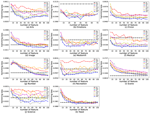
Fig. 1: Hamming Loss comparisions of 8 feature selection algorithms on 11 datasets.

Usually, the neighborhood graph in the manifold regularization term is obtained directly through KNN [3, 4, 9, 23, 31], so it is difficult to avoid the occurrence of ”short circuit”, especially on the data set like ”Swiss Roll”. In supervised learning, especially in multi-label learning, the cost of obtaining labels is very expensive, but methods such as MSSL and MDFS only use label information once when training models, which leads to the waste of label information. Different from the above method, we first construct a joint similarity matrix using the information of labels and features, and then implement multi-step random walk based on this matrix to obtain the neighborhood graph. Joint similarity matrix can avoid ”short circuit” phenomenon to a great extent, and random walk strategy can further improve the robustness of neighborhood graph to outliers. In addition, we only need to select a small number of random walk steps to get a highly sparse neighborhood graph, which greatly improves the computational efficiency.

The specific steps to obtain the neighborhood graph are as follows:

step1: Calculate the Euclidean distance matrix betwwen instances based on the features of instance $Dist=(d_{ij})$, where $d_{ij}={\|x_{i}-x_{j}\|}_{2},\quad\forall i,j=1,2,\dots,n$.

step2: Calculate the Gaussian adjacency weight matrix $V=(v_{ij})$, where $v_{ij}=e^{-\frac{d_{ij}^{2}}{\sigma^{2}}},\quad\forall i,j=1,2,...,n$.

Fig. 2: Ranking Loss comparisions of 8 feature selection algorithms on 11 datasets.

step3: Calculate Jaccard Index matrix $R=(r_{ij})$ between samples based on labels.

$$r_{ij}=\begin{cases}\frac{y_{i}y_{j}^{T}}{y_{i}y_{i}^{T}+y_{j}y_{j}^{T}-y_{i}y_{j}^{T}},&i\neq j\\ 0,&otherwise.\end{cases}$$ (3)

step4: Calculate the joint similarity matrix $T=V\odot R$, the symbol $\odot$ represents the Hadamard product, that is $T_{ij}=V_{ij}\cdot R_{ij},\quad\forall i,j=1,2,\dots,n$.

step5: Starting from node $i$, implement one-step random walk according to probability $P_{i}$, where $P=D^{-1}T$, $D$ is a diagonal matrix and satisfies $D_{ii}=\sum\limits_{j}T_{ij},\quad\forall i=1,2,\dots,n$. If it reaches the node $j$, then implement a one-step random walk with probability $P_{j}$ and repeat $k$ times like this.

The counting matrix $C$ can be obtained by recording the times that it passes through other nodes when starting from node $i$. We only need to make $S=(C+C^{T})/2$ to get a highly robust neighborhood graph based on the joint structure and random walk strategy. Algorithm description please refer to Algorithm 1.

Algorithm 1: Neighborhood Graph Algorithm (DFS and BFS)

Input: feature matrix $X\in\mathbb{R}^{n\times p}$, label matrix $Y\in\mathbb{R}^{n\times m}$.

Output: Neighborhood Graph $S$.

Calculate one-step transform probability matrix $P$.

Initialize $C$ as a $n\times n$ zero matrix.

For $i=1:n$

Set $x_{0}=x_{i}$, $P_{0}=P_{i}$

If DFS:

For $s=1:k$

Implement one-step random walk that starts from $x_{0}$ with the possibility of $P_{0}$.

If it reached node $x_{j}$, then $c_{ij}=c_{ij}+1$.

Set $p_{ji}=0$ and renormalized $P_{j}$, so that $\sum\limits_{i}p_{ji}=1$.

Set $x_{0}=x_{j},P_{0}=P_{j}$

If BFS:

For $s=1:k$

Implement one-step random walk that starts from $x_{0}$

with the possibility of $P_{0}$.

If it reached node $x_{j}$, then $c_{ij}=c_{ij}+1$.

Set $S=(C+C^{T})/2$

Notes: DFS and BFS are abbreviations for Depth-First Search and Breadth-First Search, respectively.

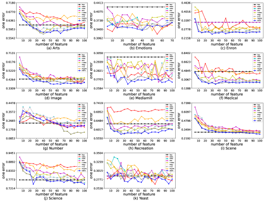
Fig. 3: One Error comparisions of 8 feature selection algorithms on 11 datasets.

The neighborhood graph obtained by algorithm 1 not only has symmetry and sparsity, but also has strong robustness to outliers. In fact, carrying out random walks is equivalent to carrying out weighted random sampling, in which the weight of abnormal samples is 0 or very small.

By applying $\ell_{2,1}$ regularization to the coefficient matrix, it will become row sparse, thus realizing feature selection.

$$SR_{1}(W)={\|W\|}_{2,1}$$ (4)

On the other hand, multicollinearity of features usually exists in high dimensional data sets. However, this effect can be reduced by imposing a quadratic penalty term, so we consider using Frobenius regularization term in the model at the same time.

$$SR_{2}(W)={\|W\|}_{F}^{2}$$ (5)

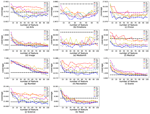
Fig. 4: Coverage comparisions of 8 feature selection algorithms on 11 datasets.

Inspired by the elastic net method, we construct a joint regularization term by introducing the factor $\rho$, which can balance the effects of $SR_{1}(W)$ and $SR_{2}(W)$. The model considers not only the action of a single feature, but also the joint action of a group of features.

$$\begin{split}SR(W)&=\rho SR_{1}(W)+(1-\rho)SR_{2}(W)\\ &=\rho{\|W\|}_{2,1}+(1-\rho){\|W\|}_{F}^{2}\end{split}$$ (6)

where ${\|W\|}_{2,1}$ is not continuous and differentiable, so we need to find an approximate solution. Due to

$${\|W\|}_{2,1}=\sum\limits_{i=1}^{p}\sqrt{\sum\limits_{j=1}^{m}W_{ij}^{2}}=\sum\limits_{i=1}^{p}\|w_{i}\|_{2}=\sum\limits_{i=1}^{p}(w_{i}w_{j}^{T})^{\frac{1}{2}}$$ (7)

and when $\forall i=1,2,\dots,p$ satisfies $w_{i}\neq 0$. Therefore, the following formula always holds

$$\begin{split}\frac{\partial{\|W\|}_{2,1}}{\partial W}&=\frac{\partial{\sum\limits_{i=1}^{p}(w_{i}w_{j}^{T})^{\frac{1}{2}}}}{\partial{w_{j}}}=2UW\\ &=\frac{\partial{tr(W^{T}UW)}}{\partial{W}}\end{split}$$ (8)

That is $\|W\|_{2,1}-tr(W^{T}UW)$ is an constant that can be omited in object function, so approximately there can be

$${\|W\|}_{2,1}=tr(W^{T}UW)$$ (9)

Here $U$ is a diagonal matrix, and its $i$-th element is $U_{ii}=1/max\{2{\|w_{i}\|}_{2},\varepsilon\}$, $\varepsilon$ is a sufficiently small positive constant such that the denominator is never equal to 0.

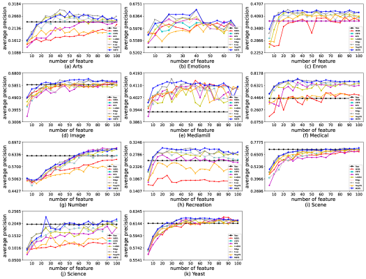
Fig. 5: Average Precision comparisions of 8 feature selection algorithms on 11 datasets.

Based on the above, we get the following optimization problem

$$\begin{split}\min\limits_{W,b}&\frac{1}{2}{\|XW+1_{n}b-Y\|}_{F}^{2}+\frac{\alpha}{2}\cdot\frac{1}{2}\sum\limits_{i,j}{\|x_{i}W-x_{j}W\|}_{2}^{2}S_{ij}+\frac{\beta}{2}(\rho{\|W\|}_{2,1}+(1-\rho){\|W\|}_{F}^{2})\end{split}$$ (10)

Using the trace of the matrix to reformulate the above formula as follows

$$\begin{split}\min\limits_{W,b}&\frac{1}{2}tr(W^{T}X^{T}XW)+tr(b^{T}1_{n}^{T}XW)-tr(Y^{T}XW)+\frac{1}{2}tr(b^{T}1_{n}^{T}1_{n}b)-tr(Y^{T}1_{n}b)\\ +&\frac{1}{2}tr(Y^{T}Y)+\frac{\alpha}{2}tr(W^{T}X^{T}LXW)+\frac{\beta\rho}{2}tr(W^{T}UW)+\frac{\beta\left(1-\rho\right)}{2}tr(W^{T}W)\end{split}$$ (11)

4 Optimization algorithm and analysis

4.1 Optimization algorithm

May wish to write the formula (9) as $f(W,b)$, then we can solve b and W by using alternating least squares(ALS) methods.

(1) Fixed W and U, Update b

$$b=\frac{1}{n}(1_{n}^{T}Y-1_{n}^{T}XW)$$ (12)

(2) Fixed U and b, Update W

$$W={(X^{T}(H+\alpha L)X+\beta(1-\rho)I_{p}+\beta\rho U)}^{-1}X^{T}HY$$ (13)

where $H=I_{n}-\frac{1}{n}1_{n}1_{n}^{T}$.

(3) Fixed W and b, Update U

$$U_{i,i}=\frac{1}{max\{2\|w_{i}\|_{2},\varepsilon\}}$$ (14)

The description of the optimization algorithm corresponding to the above process please refer to the Algorithm2.

Algorithm 2: Random Manifold Sampling and Joint Sparse Regularization for Multi-label Feature Selection

Input: feature matrix: $X\in\mathbb{R}^{n\times p}$, label matrix: $Y\in\mathbb{R}^{n\times m}$, # of select feature: $l$, parameter: $\alpha,\beta,\rho$.

Output: the set of select features: $SF$.

Calculate the neighborhood graph S according to Algorithm 1.

Calculate the graph Laplacian matrix of the sample graph $L$.

Calculate the centering matrix $H=I_{n}-1_{n}1_{n}^{T}/n$.

Set $t=0,\quad\varepsilon=1\times 10^{-64}$.

Random initializing $U$ as a diagonal matrix.

While not convergence

Update $W$ as $W^{(t+1)}$ according to the formula (13).

Update $U$ as $U^{(t+1)}$ according to the formula (14).

$t=t+1$.

Until convergence

Calculate features weight vector $scores$, where $scores_{i}={\|w_{i}\|}_{2}$.

Select the top $l$ features with the highest score.

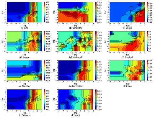
Fig. 6: Average Precision of MSFS when $\alpha$ and $\beta$ varies from $10^{-5}$ to $10^{3}$, the number of feature set as 50.

4.2 Complexity analysis

We denote $n,p$ and $m$ as the number of instances, features and labels respectively, $k$ and $t$ are the number of random walk steps and iterations. In general, $n>p>m$, $k=80$, and $t\leq 50$ are satisfied. Therefore, the complexity of algorithm 1 is $O((p+m)n^{2}+(p+m+k)n)$, and the computational complexity of each iteration of algorithm 2 is $O(pn^{2}+(p^{2}+mp)n+p^{3}+p^{2}+mp)$. Therefore, the total complexity of our algorithm is $O((p+m)n^{2}+(p+m+k)n)+O(t(pn^{2}+(p^{2}+mp)n+p^{3}+p^{2}+mp))=O(n^{2}p+np^{2}+p^{3})$.

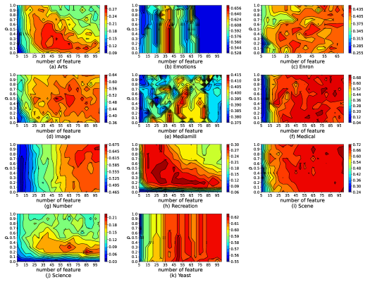
Fig. 7: Average Precision of MSFS when $\rho$ varies from 0.0 to 1.0 and the number of feature varies from 5 to 100 (70 for emotions).

4.3 Convergence analysis

In this section, we will prove the convergence of Algorithm 2. Before the proof, we need to introduce a lemma.

Lemma 1.

For any $a>0,b>0$, the following inequality always holds

$$\sqrt{a}-\frac{a}{2\sqrt{b}}\leq\sqrt{b}-\frac{b}{2\sqrt{b}}$$ (15)

Theorem 1.

Algorithm 2 gives the optimal solution with convexity.

Proof:.

If we write $W^{(t+1)},b^{(t+1)}$ as the solution produced in the $t$-th iteration, we can get the following relationship

$$\begin{split}\left(W^{(t+1)},b^{(t+1)}\right)&=\arg\min\limits_{W,b}\frac{1}{2}{\left\|XW+1_{n}b-Y\right\|}_{F}^{2}+\frac{\alpha}{2}tr\left(W^{T}X^{T}LXW\right)+\frac{\beta\left(1-\rho\right)}{2}tr\left(W^{T}W\right)+\frac{\beta\rho}{2}tr\left(W^{T}U^{(t)}W\right)\end{split}$$ (16)

Here $U^{(t)}$ is a diagonal matrix, and its $i$-th diagonal element is $\frac{1}{2{\left\|w_{i}^{(t)}\right\|}_{2}}$, so the following formula can be obtained.

$$\begin{split}&\frac{1}{2}{\left\|XW^{(t+1)}-1_{n}b^{(t+1)}-Y\right\|}_{F}^{2}+\frac{\alpha}{2}tr\left({\left(W^{(t+1)}\right)}^{T}X^{T}LXW^{(t+1)}\right)+\frac{\beta\left(1-\rho\right)}{2}tr\left({\left(W^{(t+1)}\right)}^{T}W\right)\\ &+\frac{\beta\rho}{2}tr\left({\left(W^{(t+1)}\right)}^{T}U^{t}W^{(t+1)}\right)\leq\frac{1}{2}{\left\|XW^{(t)}-1_{n}b^{(t)}-Y\right\|}_{F}^{2}+\frac{\alpha}{2}tr\left({\left(W^{(t)}\right)}^{T}X^{T}LXW^{(t)}\right)\\ &+\frac{\beta\left(1-\rho\right)}{2}tr\left({\left(W^{(t)}\right)}^{T}W\right)+\frac{\beta\rho}{2}tr\left({\left(W^{(t)}\right)}^{T}U^{t}W^{(t)}\right)\end{split}$$ (17)

Further, there is

$$\begin{split}&\frac{1}{2}{\left\|XW^{(t+1)}-1_{n}b^{(t+1)}-Y\right\|}_{F}^{2}+\frac{\alpha}{2}tr\left({\left(W^{(t+1)}\right)}^{T}X^{T}LXW^{(t+1)}\right)+\frac{\beta\left(1-\rho\right)}{2}tr\left({\left(W^{(t+1)}\right)}^{T}W\right)+\frac{\beta\rho}{2}\sum\limits_{i}\frac{{\left\|w_{i}^{(t+1)}\right\|}_{2}^{2}}{2{\left\|w_{i}^{(t)}\right\|}_{2}}\\ &\leq\frac{1}{2}{\left\|XW^{(t)}-1_{n}b^{(t)}-Y\right\|}_{F}^{2}+\frac{\alpha}{2}tr\left({\left(W^{(t)}\right)}^{T}X^{T}LXW^{(t)}\right)+\frac{\beta\left(1-\rho\right)}{2}tr\left({\left(W^{(t)}\right)}^{T}W\right)+\frac{\beta\rho}{2}\sum\limits_{i}\frac{{\left\|w_{i}^{(t)}\right\|}_{2}^{2}}{2{\left\|w_{i}^{(t)}\right\|}_{2}}\end{split}$$ (18)

Therefore, it can be inferred that the following formula holds

$$\begin{split}&\frac{1}{2}{\left\|XW^{(t+1)}-1_{n}b^{(t+1)}-Y\right\|}_{F}^{2}+\frac{\alpha}{2}tr\left({\left(W^{(t+1)}\right)}^{T}X^{T}LXW^{(t+1)}\right)+\frac{\beta\left(1-\rho\right)}{2}tr\left({\left(W^{(t+1)}\right)}^{T}W\right)+\frac{\beta\rho}{2}{\left\|W^{(t+1)}\right\|}_{2,1}\\ &-\frac{\beta\rho}{2}\left({\left\|W^{(t+1)}\right\|}_{2,1}-\sum\limits_{i}\frac{{\left\|w_{i}^{(t+1)}\right\|}_{2}^{2}}{2{\left\|w_{i}^{(t)}\right\|}_{2}}\right)\leq\frac{1}{2}{\left\|XW^{(t)}-1_{n}b^{(t)}-Y\right\|}_{F}^{2}+\frac{\alpha}{2}tr\left({\left(W^{(t)}\right)}^{T}X^{T}LXW^{(t)}\right)\\ &+\frac{\beta\left(1-\rho\right)}{2}tr\left({\left(W^{(t)}\right)}^{T}W\right)+\frac{\beta\rho}{2}{\left\|W^{(t)}\right\|}_{2,1}-\frac{\beta\rho}{2}\left({\left\|W^{(t)}\right\|}_{2,1}-\sum\limits_{i}\frac{{\left\|w_{i}^{(t)}\right\|}_{2}^{2}}{2{\left\|w_{i}^{(t)}\right\|}_{2}}\right)\end{split}$$ (19)

From ${\|W\|}_{2,1}=\sum\limits_{i}{\|w_{i}\|}_{2}$ and the Lemma 1

$${\|w_{i}^{(t+1)}\|}_{2}-\frac{{\|w_{i}^{(t+1)}\|}_{2}^{2}}{2{\|w_{i}^{(t)}\|}_{2}}\leq{\|w_{i}^{(t)}\|}_{2}-\frac{{\|w_{i}^{(t)}\|}_{2}^{2}}{2{\|w_{i}^{(t)}\|}_{2}}$$ (20)

Thus

$$\sum\limits_{i}{\left({\|w_{i}^{(t+1)}\|}_{2}-\frac{{\|w_{i}^{(t+1)}\|}_{2}^{2}}{2{\|w_{i}^{(t)}\|}_{2}}\right)}\leq\sum\limits_{i}{\left({\|w_{i}^{(t)}\|}_{2}-\frac{{\|w_{i}^{(t)}t\|}_{2}^{2}}{2{\|w_{i}^{(t)}\|}_{2}}\right)}$$ (21)

That is

$${\|W^{(t+1)}\|}_{2,1}-\sum\limits_{i}\frac{{\|w_{i}^{(t+1)}\|}_{2}^{2}}{2{\|w_{i}^{(t)}\|}_{2}}\leq{\|W^{(t)}\|}_{2,1}-\sum\limits_{i}\frac{{\|w_{i}^{(t)}\|}_{2}^{2}}{2{\|w_{i}^{(t)}\|}_{2}}$$ (22)

Therefore we can immediately infer that the algorithm converges. ∎

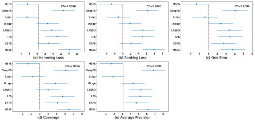
Fig. 8: Comparison of MSFS against other comparing methods with the Bonferroni-Dunn test($\alpha=0.05$).

5 Experiments and results

In this section, a series of compared experiments are designed in six publicly available data sets. Experimental results show that the proposed method achieves state-of-art on multiple data sets. It should be noted that in the experiments involved in this paper, ML-KNN is used as the basic classifier.

5.1 Datasets

We experimented with 11 datasets for descriptions in Table 1, all of which are freely available from the open source multi-label learning data site but the Number. The data set of Number is made manually, and it contains 2000 pieces of data. Each piece of data consists of five digital pictures containing 81 pixels, and some of the five pictures may not contain numbers. In order to make the classifier trained from the data set more robust, we add 15% Gaussian noise to each data set.

Table 1: Data sets and the related descriptions

Datasets	Dim(D)	L(D)	$\|$D$\|$	$\|$train$\|$	$\|$test$\|$	PMC	ANL	Dens
Arts	462	26	5000	2000	3000	0.4398	1.6360	0.0629
Emotions	72	6	593	391	202	0.6998	1.8685	0.3114
Enron	1001	53	1702	1123	579	0.8848	3.3784	0.0637
Image	294	5	2000	1000	1000	0.2285	1.2360	0.2472
Mediamil	120	101	15730	5000	10730	0.9350	4.3756	0.0433
Medical	1449	45	978	333	645	0.2311	1.2454	0.0277
Number	405	10	2000	1000	1000	0.9825	3.3265	0.3326
Recreation	606	22	5000	2000	3000	0.3080	1.4232	0.0647
Scene	294	6	2407	1211	1196	0.0735	1.0740	0.1790
Science	743	40	5000	2000	3000	0.3228	1.4506	0.0363
Yeast	103	14	2417	1500	917	0.9868	4.2371	0.3026
(http://mulan.sourceforge.net/datasets-mlc.html)

Here, Dim(D) is the dimension of the corresponding data set, that is, the number of features. L(D) is the number of labels, $\|$D$\|$ is the number of instances of the data set. PMC, ANL and Dens are defined as follows:

(1) $PMC=\frac{1}{n}\sum\limits_{i=1}^{n}\{y_{i}y_{i}^{T}\geq 2\}$, which measures the percentage of documents belonging to more than one category.

(2) $ANL=\frac{1}{n}\sum\limits_{i=1}^{n}|y_{i}|$, which denotes the average number of labels that each object belongs to.

(3) $Dens=\frac{1}{nm}\sum\limits_{i=1}^{n}|y_{i}|$, which measures the density of the label distribution of the dataset.

5.2 Evaluation metrics

In multi-label learning, we pay more attention to the ranking of prediction results, so we use hamming loss, ranking loss, one error, coverage and average precision as the evaluation metrics of multi-label feature selection.

(1) Hamming Loss measures the ratio of incorrectly predicted labels.

$$HL=\frac{1}{n}\sum\limits_{i=1}^{n}\frac{\hat{y}_{i}\oplus y_{i}}{m}$$ (23)

(2) Ranking Loss evaluates the average fraction of label pairs that irrelevant labels are ranked higher than the relevant label.

$$RL=\frac{1}{n}\sum\limits_{i=1}^{n}\frac{|\left\{\left(l_{k},l_{j}\right)|f_{k}\left(x_{i}\right)<f_{j}\left(x_{i}\right),\left(l_{k},l_{j}\in y_{i}\times\bar{y_{i}}\right)\right\}|}{\left|y_{i}\right|\left|\bar{y_{i}}\right|}$$ (24)

(3) One Error evaluates how many times the top-ranked label is not in the relevant label set of the instance.

$$OE=\frac{1}{n}\sum\limits_{i=1}^{n}\left(arg\max\limits_{l_{k}\in y_{i}}rank\left(x_{i},l_{k}\right)\notin y_{k}\right)$$ (25)

(4) Coverage is used to measure the steps, on average, required to cover the true label.

$$Cov=\frac{1}{m}\left(\frac{1}{n}\sum\limits_{i=1}^{n}arg{\max\limits_{l_{k}\in y_{i}}}rank\left(x_{i},l_{k}\right)-1\right)$$ (26)

(5) Average Precision evaluates the average fraction of labels ranked above a particular label in the truth label sets.

$$AP=\frac{1}{n}\sum\limits_{i=1}^{n}\frac{1}{y_{i}}\sum\limits_{l_{k}\in y_{i}}\frac{\left\{l_{j}|rank\left(x_{i},l_{j}\right)\leq rank\left(x_{i},l_{k}\right),l_{j}\in y_{i}\right\}}{rank\left(x_{i},l_{k}\right)}$$ (27)

(6) The difference between two methods is distinguished with the critical difference (CD), as follow

$$CD=q_{\alpha}\sqrt{\frac{k(k+1)}{6N}}$$ (28)

where $q_{\alpha}=2.690$ at significance level $\alpha=0.05$, and then we can calculate CD = 2.8096 (k = 8, N = 11).

When using hamming loss, ranking loss, one error, coverage to evaluate, the smaller the value, the better the model performance, whereas on AP the opposite is true.

5.3 Experiment setting

In order to verify the effectiveness of the proposed method, we make a comprehensive comparison with the following methods.

Base: All original features are selected for learning tasks, the base classifier is ML-KNN [34].

RFS [21]: By imposing $\ell_{2,1}$ penalty on the loss function, the coefficient matrix with row sparse property is obtained, thus completing feature selection in multi-label learning.

MSSL [4]: The method combines multi-label learning and manifold learning. It treats each feature as a node and constructs the graph Laplacian matrix.

CSFS [5]: CSFS extends the algorithm to semi-supervised learning by weighting samples, which makes the model can be applied to large-scale data sets

LASSO [26]: It use the $\ell_{1}$ regularization to make elements of the coefficient matrix become 0 as much as possible.

Ridge [10]: By imposing $\ell_{2}$ penalty on the coefficients, Ridge method makes the weights of variables with linear correlation decrease at the same time, thus weakening the adverse consequences caused by multiple linearity.

E-net [35]: It makes the model have the ability to select a single strong feature and a group of strong features by balancing $\ell_{1}$ and $\ell_{2}$ regularization.

DeepFS : Under the background of deep learning, it can learn a large number of parameters by building a multi-layer network to evaluate the importance of features to labels. (We completed the experiment by referring to python’s dl-selection library)

For the sake of fairness, all of the parameters of the above mentioned methods for comparative experiments are generally set as $\{10^{-5},10^{-4},10^{-3},10^{-2},\\ 10^{-1},1,10^{1},10^{2},10^{3}\}$, and the iteration times of the algorithm are consistently set as 50. Specifically, for MLKNN, we set k=7, for E-net and our proposed MSFS, we set the value interval of $\rho$ as $\{0.0,0.1,0.2,0.3,0.4,0.5,0.6,0.7,0.8,0.9,\\ 1.0\}$. In addition, the length of random walk is set as 80 for MSFS. In the DeepFS, the number of layers and dimensions of the hidden layers of the neural network are selected from [2, 4, 8, 16] and [512, 256, 128, 64, 32].

5.4 Comparison and analysis of methods

We conducted comparative experiments on 11 data sets, and we selected {5, 10, 15,…,90, 95, 100} for the number of features. For each method, we obtained its best performance through grid search and recorded it in the following tables. Table 2, 3, 4, 5, and 6 are the recorded results of hamming loss, ranking loss, one error, coverage, and average precision, respectively. In these table, we use bold font to indicate the best performance.

Table 2: Hamming loss(mean$\pm$std) of 8 different algorithms on 11 different datasets

Datasets	Base	MSSL	CSFS	RFS	LASSO	Ridge	E-net	DeepFS	MSFS
Arts	0.0580	0.0582$\pm$0.0014	0.0564$\pm$0.0016	0.0572$\pm$0.0011	0.0561$\pm$0.0020	0.0564$\pm$0.0013	0.0557$\pm$0.0015	0.0581$\pm$0.0017	0.0557$\pm$0.0014
Emotions	0.2979	0.2252$\pm$0.0096	0.2178$\pm$0.0060	0.2219$\pm$0.0061	0.2145$\pm$0.0073	0.2145$\pm$0.0072	0.2046$\pm$0.0062	0.2244$\pm$0.0053	0.2046$\pm$0.0048
Enron	0.0511	0.0505$\pm$0.0013	0.0488$\pm$0.0010	0.0511$\pm$0.0012	0.0487$\pm$0.0013	0.0488$\pm$0.0015	0.0483$\pm$0.0012	0.0491$\pm$0.0012	0.0478$\pm$0.0009
Image	0.1832	0.1802$\pm$0.0072	0.1728$\pm$0.0050	0.1776$\pm$0.0038	0.1802$\pm$0.0057	0.1728$\pm$0.0057	0.1728$\pm$0.0049	0.1790$\pm$0.0051	0.1712$\pm$0.0031
Mediamill	0.0322	0.0318$\pm$0.0011	0.0317$\pm$0.0010	0.0317$\pm$0.0011	0.0318$\pm$0.0010	0.0317$\pm$0.0010	0.0316$\pm$0.0008	0.0318$\pm$0.0010	0.0317$\pm$0.0004
Medical	0.0200	0.0168$\pm$0.0006	0.0125$\pm$0.0003	0.0128$\pm$0.0003	0.0129$\pm$0.0004	0.0125$\pm$0.0005	0.0119$\pm$0.0003	0.0168$\pm$0.0005	0.0111$\pm$0.0003
Number	0.1921	0.2026$\pm$0.0078	0.1889$\pm$0.0054	0.1679$\pm$0.0052	0.1743$\pm$0.0032	0.1889$\pm$0.0054	0.1693$\pm$0.0037	0.2176$\pm$0.0041	0.1722$\pm$0.0033
Recreation	0.0580	0.0601$\pm$0.0020	0.0561$\pm$0.0014	0.0564$\pm$0.0015	0.0562$\pm$0.0016	0.0561$\pm$0.0016	0.056$\pm$0.0015	0.0573$\pm$0.0015	0.0558$\pm$0.0012
Scene	0.0924	0.1038$\pm$0.0038	0.1016$\pm$0.0023	0.1073$\pm$0.0027	0.0973$\pm$0.0030	0.1016$\pm$0.0031	0.0962$\pm$0.0025	0.0971$\pm$0.0025	0.0964$\pm$0.0016
Science	0.0337	0.0345$\pm$0.0007	0.0331$\pm$0.0008	0.0338$\pm$0.0008	0.0334$\pm$0.0009	0.0331$\pm$0.0013	0.0328$\pm$0.0009	0.0337$\pm$0.0011	0.0331$\pm$0.0008
Yeast	0.1960	0.194$\pm$0.0062	0.1949$\pm$0.0050	0.1942$\pm$0.0053	0.1942$\pm$0.0059	0.1949$\pm$0.0072	0.1934$\pm$0.0050	0.1942$\pm$0.0063	0.1931$\pm$0.0047
The smaller the value, the better the performs

Table 3: Ranking loss(mean$\pm$std) of 8 different algorithms on 11 different datasets

Datasets	Base	MSSL	CSFS	RFS	LASSO	Ridge	E-net	DeepFS	MSFS
Arts	0.0335	0.0341$\pm$0.0009	0.0327$\pm$0.0009	0.0335$\pm$0.0009	0.0321$\pm$0.0010	0.0327$\pm$0.0010	0.0314$\pm$0.0006	0.0346$\pm$0.0010	0.0317$\pm$0.0010
Emotions	0.1824	0.1555$\pm$0.0052	0.1553$\pm$0.0045	0.1516$\pm$0.0025	0.1524$\pm$0.0057	0.1524$\pm$0.0037	0.1424$\pm$0.0039	0.1497$\pm$0.0042	0.1424$\pm$0.0037
Enron	0.0150	0.0144$\pm$0.0004	0.0143$\pm$0.0004	0.0150$\pm$0.0003	0.0144$\pm$0.0004	0.0143$\pm$0.0004	0.0143$\pm$0.0003	0.0143$\pm$0.0004	0.0142$\pm$0.0004
Image	0.1579	0.1516$\pm$0.0049	0.1456$\pm$0.0038	0.1472$\pm$0.0036	0.1539$\pm$0.0054	0.1456$\pm$0.0046	0.1446$\pm$0.0042	0.1481$\pm$0.0045	0.1408$\pm$0.0028
Mediamill	0.0071	0.0070$\pm$0.0000	0.0070$\pm$0.0000	0.0070$\pm$0.0000	0.0071$\pm$0.0000	0.0070$\pm$0.0000	0.0070$\pm$0.0000	0.0070$\pm$0.0000	0.0070$\pm$0.0000
Medical	0.0138	0.0116$\pm$0.0004	0.0076$\pm$0.0002	0.0080$\pm$0.0002	0.0082$\pm$0.0003	0.0076$\pm$0.0002	0.0071$\pm$0.0002	0.0116$\pm$0.0002	0.0067$\pm$0.0000
Number	0.1050	0.1026$\pm$0.0037	0.1002$\pm$0.0026	0.0953$\pm$0.0025	0.0975$\pm$0.0028	0.1002$\pm$0.0035	0.0948$\pm$0.0026	0.1067$\pm$0.0031	0.0953$\pm$0.0025
Recreation	0.0391	0.0419$\pm$0.0014	0.0375$\pm$0.0009	0.0381$\pm$0.0010	0.0373$\pm$0.0005	0.0375$\pm$0.0013	0.0368$\pm$0.0010	0.0396$\pm$0.0010	0.0367$\pm$0.0009
Scene	0.0773	0.0836$\pm$0.0032	0.0763$\pm$0.0015	0.0824$\pm$0.0019	0.0788$\pm$0.0018	0.0763$\pm$0.0020	0.0775$\pm$0.0018	0.0785$\pm$0.0017	0.0756$\pm$0.0014
Science	0.0215	0.0233$\pm$0.0006	0.0212$\pm$0.0003	0.0218$\pm$0.0006	0.0214$\pm$0.0004	0.0212$\pm$0.0005	0.0211$\pm$0.0005	0.0227$\pm$0.0005	0.0207$\pm$0.0005
Yeast	0.0645	0.0634$\pm$0.0022	0.0631$\pm$0.0020	0.0638$\pm$0.0016	0.0637$\pm$0.0017	0.0631$\pm$0.0018	0.0632$\pm$0.0015	0.0639$\pm$0.0017	0.0630$\pm$0.0015
The smaller the value, the better the performs

From these tables, it can be seen that MSFS has the best performance for 35 times, ranking first, E-net (using $\ell_{1}$ and $\ell_{2}$ regularization at the same time) 12 times, ranking second, MSSL (using manifold regularization) and RFS (only using $\ell_{2,1}$ regularization) 2 times, ranking third. We can get the following several conclusions. First of all, even if E-net only uses joint sparse regularization, it is far superior to other methods, which shows that joint sparse regularization method has better feature selection ability than other methods. Secondly, when only $\ell_{2,1}$ regularization is used, RFS method does not perform well, that is, $\ell_{2,1}$ regularization alone does not have strong feature selection ability. Then, after introducing manifold regularization on the basis of $\ell_{2,1}$ regularization, MSSL method is superior to RFS, which shows that manifold regularization can improve sparse regularization. Next, the proposed method is superior to E-net method because it uses manifold regularization to obtain more accurate spatial structure. Compared with the MSSL method, we use the joint sparse regularization method to obtain more discriminant features. Finally, although various neural network models have excellent performance in feature extraction and prediction, their ability is not outstanding in the field of feature selection, which is due to it lack of interpretation of original features to some extent.

Table 4: One Error(mean$\pm$std) of 8 different algorithms on 11 different datasets

Datasets	Base	MSSL	CSFS	RFS	LASSO	Ridge	E-net	DeepFS	MSFS
Arts	0.6160	0.6170$\pm$0.0187	0.5888$\pm$0.0185	0.6092$\pm$0.0170	0.5801$\pm$0.0190	0.5888$\pm$0.0247	0.5731$\pm$0.0144	0.6347$\pm$0.0223	0.5767$\pm$0.0134
Emotions	0.4257	0.3218$\pm$0.0095	0.3416$\pm$0.007	0.3465$\pm$0.0074	0.3465$\pm$0.0105	0.3416$\pm$0.0096	0.3366$\pm$0.0072	0.3366$\pm$0.0111	0.3366$\pm$0.0075
Enron	0.3276	0.2790$\pm$0.0094	0.2530$\pm$0.0067	0.3276$\pm$0.0058	0.2669$\pm$0.0056	0.2530$\pm$0.0093	0.2530$\pm$0.0054	0.2686$\pm$0.0061	0.2444$\pm$0.0071
Image	0.4300	0.3940$\pm$0.0144	0.3860$\pm$0.0079	0.3840$\pm$0.0094	0.4080$\pm$0.0122	0.3860$\pm$0.0146	0.3860$\pm$0.0101	0.3940$\pm$0.0120	0.3750$\pm$0.0069
Mediamill	0.3003	0.2708$\pm$0.0094	0.2688$\pm$0.0076	0.2668$\pm$0.0057	0.2737$\pm$0.0096	0.2688$\pm$0.0097	0.2657$\pm$0.0069	0.2713$\pm$0.0093	0.2639$\pm$0.0074
Medical	0.4667	0.4124$\pm$0.0177	0.2372$\pm$0.0051	0.2651$\pm$0.0085	0.2744$\pm$0.0092	0.2372$\pm$0.0064	0.2202$\pm$0.0051	0.3984$\pm$0.0089	0.2109$\pm$0.0059
Number	0.2410	0.1910$\pm$0.0050	0.2280$\pm$0.0069	0.2040$\pm$0.0061	0.1270$\pm$0.0025	0.2280$\pm$0.0066	0.1270$\pm$0.0026	0.2410$\pm$0.0071	0.1990$\pm$0.0042
Recreation	0.6316	0.6934$\pm$0.0244	0.5897$\pm$0.0121	0.6014$\pm$0.0123	0.5930$\pm$0.0180	0.5897$\pm$0.0158	0.5769$\pm$0.0132	0.6300$\pm$0.0165	0.5766$\pm$0.0157
Scene	0.3094	0.3294$\pm$0.0122	0.3060$\pm$0.0102	0.3135$\pm$0.0075	0.2993$\pm$0.0117	0.3060$\pm$0.0115	0.2826$\pm$0.0051	0.3052$\pm$0.0107	0.2793$\pm$0.0075
Science	0.7748	0.8436$\pm$0.0192	0.7562$\pm$0.0173	0.7802$\pm$0.0182	0.7685$\pm$0.0241	0.7562$\pm$0.0270	0.7525$\pm$0.0169	0.8175$\pm$0.0252	0.7472$\pm$0.0119
Yeast	0.2868	0.2639$\pm$0.0069	0.2824$\pm$0.0072	0.2726$\pm$0.0056	0.2792$\pm$0.0091	0.2726$\pm$0.0098	0.2770$\pm$0.0073	0.2715$\pm$0.0081	0.2650$\pm$0.0042
The smaller the value, the better the performs

Table 5: Coverage(mean$\pm$std) of 8 different algorithms on 11 different datasets

Datasets	Base	MSSL	CSFS	RFS	LASSO	Ridge	E-net	DeepFS	MSFS
Arts	15.6163	15.7259$\pm$0.5128	14.9189$\pm$0.3834	15.3060$\pm$0.4891	14.5818$\pm$0.4101	14.9189$\pm$0.5891	14.2577$\pm$0.2842	15.7081$\pm$0.5573	14.5375$\pm$0.3391
Emotions	3.0050	2.5594$\pm$0.0664	2.5396$\pm$0.0752	2.5347$\pm$0.0682	2.5248$\pm$0.0820	2.5248$\pm$0.0911	2.4554$\pm$0.0528	2.5842$\pm$0.0967	2.4505$\pm$0.0572
Enron	24.6118	23.5511$\pm$0.6208	23.0485$\pm$0.5181	24.6118$\pm$0.5306	22.9792$\pm$0.6218	23.0485$\pm$0.7633	22.7106$\pm$0.5541	23.1057$\pm$0.7528	22.7106$\pm$0.6515
Image	1.4060	1.3910$\pm$0.0467	1.3470$\pm$0.0359	1.3570$\pm$0.0276	1.3940$\pm$0.0454	1.3470$\pm$0.0458	1.3400$\pm$0.0326	1.3690$\pm$0.0501	1.2960$\pm$0.0355
Mediamill	70.2928	63.6074$\pm$2.0855	64.1155$\pm$1.7667	64.2577$\pm$1.5544	62.9520$\pm$1.2791	64.1155$\pm$1.902	62.9520$\pm$1.6103	63.6138$\pm$1.8578	62.6714$\pm$1.5689
Medical	16.9302	14.4264$\pm$0.4000	9.0791$\pm$0.1957	9.7659$\pm$0.2945	9.6899$\pm$0.2941	9.0791$\pm$0.2437	7.9609$\pm$0.2066	13.8682$\pm$0.3126	8.0465$\pm$0.1872
Number	5.6820	5.7080$\pm$0.2242	5.9130$\pm$0.1587	5.5910$\pm$0.1196	5.3460$\pm$0.1401	5.9130$\pm$0.2253	5.3460$\pm$0.1327	6.0330$\pm$0.2094	5.5920$\pm$0.1305
Recreation	10.5960	11.1007$\pm$0.4260	10.5685$\pm$0.2963	10.7797$\pm$0.2810	10.5010$\pm$0.3758	10.5685$\pm$0.3901	10.3472$\pm$0.2946	10.8449$\pm$0.3536	10.4503$\pm$0.2893
Scene	0.9264	0.9331$\pm$0.0353	0.9373$\pm$0.0273	0.9816$\pm$0.0252	0.8946$\pm$0.0278	0.9373$\pm$0.0316	0.8654$\pm$0.0156	0.8896$\pm$0.0337	0.8620$\pm$0.0148
Science	21.8863	23.0467$\pm$0.7623	21.5680$\pm$0.5938	22.3369$\pm$0.4698	21.6064$\pm$0.7420	21.5680$\pm$0.6806	21.6064$\pm$0.5425	22.6348$\pm$0.6258	21.4239$\pm$0.4758
Yeast	9.1897	8.7219$\pm$0.3227	8.7917$\pm$0.2827	8.6565$\pm$0.1905	8.7852$\pm$0.2423	8.7917$\pm$0.2744	8.7634$\pm$0.1849	8.6917$\pm$0.2659	8.6401$\pm$0.1575
The smaller the value, the better the performs

Table 6: Average Precision(mean$\pm$std) of 8 different algorithms on 11 different datasets

Datasets	Base	MSSL	CSFS	RFS	LASSO	Ridge	E-net	DeepFS	MSFS
Arts	0.2418	0.2303$\pm$0.0084	0.2634$\pm$0.0085	0.2418$\pm$0.0055	0.2782$\pm$0.0100	0.2634$\pm$0.0114	0.2942$\pm$0.0068	0.2177$\pm$0.0079	0.2854$\pm$0.0068
Emotions	0.5381	0.6159$\pm$0.0121	0.6155$\pm$0.0153	0.6276$\pm$0.0153	0.6344$\pm$0.0171	0.6344$\pm$0.0226	0.6572$\pm$0.0187	0.6159$\pm$0.0181	0.6572$\pm$0.0150
Enron	0.3850	0.4054$\pm$0.0145	0.4381$\pm$0.0117	0.385$\pm$0.0103	0.4303$\pm$0.0096	0.4381$\pm$0.0163	0.4424$\pm$0.0073	0.4302$\pm$0.0124	0.4396$\pm$0.0081
Image	0.5897	0.6093$\pm$0.0159	0.6219$\pm$0.0224	0.6152$\pm$0.0135	0.5945$\pm$0.0161	0.6219$\pm$0.0157	0.6272$\pm$0.0158	0.6090$\pm$0.0160	0.6362$\pm$0.0130
Mediamill	0.3930	0.4143$\pm$0.0133	0.4116$\pm$0.0138	0.4124$\pm$0.0115	0.4107$\pm$0.0124	0.4116$\pm$0.0139	0.4155$\pm$0.0088	0.4129$\pm$0.0095	0.4140$\pm$0.0084
Medical	0.4328	0.5183$\pm$0.0187	0.6961$\pm$0.0178	0.6775$\pm$0.0208	0.6711$\pm$0.0216	0.6961$\pm$0.0223	0.7163$\pm$0.0193	0.5155$\pm$0.0237	0.7321$\pm$0.0211
Number	0.6267	0.6079$\pm$0.0243	0.6314$\pm$0.0211	0.6678$\pm$0.0165	0.6595$\pm$0.0197	0.6314$\pm$0.0167	0.6642$\pm$0.0194	0.5825$\pm$0.0223	0.6619$\pm$0.0169
Recreation	0.2555	0.1997$\pm$0.0086	0.2879$\pm$0.0105	0.2769$\pm$0.0071	0.2912$\pm$0.0091	0.2879$\pm$0.0082	0.3022$\pm$0.0068	0.2472$\pm$0.0102	0.3034$\pm$0.0070
Scene	0.7027	0.6800$\pm$0.0215	0.7089$\pm$0.0170	0.6897$\pm$0.0161	0.7023$\pm$0.0251	0.7089$\pm$0.0240	0.7148$\pm$0.0170	0.7013$\pm$0.0262	0.7189$\pm$0.0136
Science	0.2018	0.1352$\pm$0.0043	0.2150$\pm$0.0070	0.1931$\pm$0.0043	0.2074$\pm$0.0073	0.2150$\pm$0.0082	0.2181$\pm$0.0039	0.1573$\pm$0.0069	0.2327$\pm$0.0042
Yeast	0.6147	0.6252$\pm$0.0148	0.6219$\pm$0.0152	0.6229$\pm$0.0124	0.6204$\pm$0.0227	0.6219$\pm$0.0197	0.6227$\pm$0.0186	0.6204$\pm$0.0182	0.6238$\pm$0.0151
The greater the value, the better the performs

In fact, we can use more label information in multi-label learning methods, instead of just calculating loss. When we construct the neighborhood graph, we integrate the information of features and labels, which makes the neighbors of samples more credible and the local structure more accurate.

To describe the performance of different methods when selecting different numbers of features on different data sets, these results are visualized. For details, please refer to Fig. 1 to Fig. 5. It can be seen that the proposed methods are among the best in almost all data sets and evaluation metrics.

Although various methods have been widely used, there are some defects at present. For example, in Fig.2 (e), the performance of each method does not improve with the increase of the number of selected features, which is mainly due to the imbalance of labels. The model will focus on predicting the primary labels, thus ignoring the secondary labels. In extreme cases, when the instances are concentrated on a few labels, the model will predict all the values of these labels as 1, while all the other labels are predicted as 0. At this time, no matter how many features are increased, their performance cannot be improved.

5.5 Sensitivity analysis

There are several parameters in the proposed method, such as $\alpha$, $\beta$, etc. We designed experiments to verify how these parameters affect the performance of the model. Figs. 6 analyze the sensitivity of Average precision to parameters $\alpha$ and $\beta$ by contour map. The darker the color, the greater the value. In Fig. 7, we fixed the parameter of $\alpha$ and $\beta$ as $0.1$ and $10$ respectively. On these data sets, it is obvious that the contour lines have shown a non-strip distribution, which is caused by selecting different $\rho$ values. The result verifies the necessity of introducing joint sparse regularization.

In addition, we have one additional parameters, the number of random walks. In fact, when we set the number of random walk steps between {30, 40, 50, 60, 70, 80}, the performance of the model is basically in a stable state, and the evaluation metrics in various aspects will not fluctuate greatly. This shows that the random walk strategy is robust and superior to other methods.

5.6 Significance test

In order to test whether the proposed method is statistically significantly superior to other methods, we performed bonferroni-dunn test, and the results are shown in Fig. 8. The results show that when the significance level is set as 0.05, MSFS is significantly superior to almost all other methods used for comparison except E-net method. Even though the statistical difference between MSFS and E-net is not significant, MSFS always performs better on the 11 data sets we experimented with.

Conclusions

In this paper, we construct a new feature selection model in the context of multi-label learning, which introduces both manifold regularization and joint sparse regularization. In the manifold regularization constraint, we combine the information of features and labels to establish a joint similarity matrix, which measures the distance between instances better and effectively avoids the occurrence of the ”short circuit”. By normalizing the rows of the joint similarity matrix, it has the properties of a random matrix. Therefore, we can implement a random walk strategy to further extract highly robust local structures. It is verified by experiments that the model can extract a stable and effcient structure with fewer transfer steps. To make the coeffcient matrix sparse, we balance the $\ell_{F}$ regularization and the $\ell_{2,1}$ regularization, so that the model can comprehensively consider the situation where multivariable work together. Compared with the previous methods, the proposed method has higher accuracy and lower loss due to introduce the joint similarity matrix and the joint sparse constraints. However, this method has a shortcoming, that is, the complexity of the algorithm is relatively higher due to the need to implement the state transition process. If the data set is very large, then the algorithm will have higher requirements on the equipment, and the effciency of the algorithm will be much lower.

In real world, data labels are often unavailable or expensive to get, which makes supervised learning hard to achieve. Therefore, our next work mainly focuses on feature selection in the field of semi-supervised learning. What’s more, the label imbalance usually seriously affects the accuracy of the inference results, so we will also consider the problem of label imbalance.

Declarations

This research did not receive any specific grant from funding agencies in the public, commercial, or not-for-profit sectors.

References

- Akbari and Hesamian [2019] M. G. Akbari, G. Hesamian, Elastic net oriented to fuzzy semiparametric regression model with fuzzy explanatory variables and fuzzy responses, IEEE Transactions on Fuzzy Systems 27 (2019) 2433–2442.
- Balasubramanian and Schwartz [2002] M. Balasubramanian, E. L. Schwartz, The isomap algorithm and topological stability, Science 295 (2002) 7–7.
- Cai et al. [2010] D. Cai, C. Zhang, X. He, Unsupervised feature selection for multi-cluster data, Proceedings of the 16th ACM SIGKDD International Conference on Knowledge Discovery and Data Mining (2010) 333–342.
- Cai and Zhu [2018] Z. Cai, W. Zhu, Multi-label feature selection via feature manifold learning and sparsity regularization, International Journal of Machine Learning and Cybernetics 9 (2018) 1321–1334.
- Chang et al. [2014] X. Chang, F. Nie, Y. Yang, H. Huang, A convex formulation for semi-supervised multi-label feature selection, Proceedings of the AAAI Conference on Artificial Intelligence 28 (2014) 1171–1177.
- Dembczyński et al. [2012] K. Dembczyński, W. Waegeman, W. Cheng, E. Hüllermeier, On label dependence and loss minimization in multi-label classification, Machine Learning 88 (2012) 5–45.
- Donoho et al. [2000] D. L. Donoho, et al., High-dimensional data analysis: The curses and blessings of dimensionality, AMS math challenges lecture 1 (2000) 32.
- Hamers et al. [1989] L. Hamers, et al., Similarity measures in scientometric research: The jaccard index versus salton’s cosine formula., Information Processing and Management 25 (1989) 315–18.
- He and Niyogi [2004] X. He, P. Niyogi, Locality preserving projections, Advances in neural information processing systems 16 (2004) 153–160.
- Hoerl and Kennard [1970] A. E. Hoerl, R. W. Kennard, Ridge regression: Biased estimation for nonorthogonal problems, Technometrics 12 (1970) 55–67.
- Huang et al. [2021] A. Huang, W. Chen, T. Zhao, C. W. Chen, Joint learning of latent similarity and local embedding for multi-view clustering, IEEE Transactions on Image Processing 30 (2021) 6772–6784.
- Johnstone and Titterington [2009] I. M. Johnstone, D. M. Titterington, Statistical challenges of high-dimensional data, Philosophical Transactions of the Royal Society A: Mathematical, Physical and Engineering Sciences 367 (2009) 4237–4253.
- Kang et al. [2006] F. Kang, R. Jin, R. Sukthankar, Correlated label propagation with application to multi-label learning, 2006 IEEE Computer Society Conference on Computer Vision and Pattern Recognition (CVPR’06) 2 (2006) 1719–1726.
- Kosub [2019] S. Kosub, A note on the triangle inequality for the jaccard distance, Pattern Recognition Letters 120 (2019) 36–38.
- Li et al. [2015] R.-H. Li, J. X. Yu, L. Qin, R. Mao, T. Jin, On random walk based graph sampling, 2015 IEEE 31st International Conference on Data Engineering (2015) 927–938.
- Li et al. [2019] Y. Li, Z. Wu, S. Lin, H. Xie, M. Lv, Y. Xu, J. C. Lui, Walking with perception: Efficient random walk sampling via common neighbor awareness, 2019 IEEE 35th International Conference on Data Engineering (ICDE) (2019) 962–973.
- Lim and Kim [2021] H. Lim, D.-W. Kim, Pairwise dependence-based unsupervised feature selection, Pattern Recognition 111 (2021) 107663.
- Lu et al. [2018] Q. Lu, X. Li, Y. Dong, Structure preserving unsupervised feature selection, Neurocomputing 301 (2018) 36–45.
- Laurens van der Maaten [2008] G. H. Laurens van der Maaten, Visualizing data using t-sne., Journal of machine learning research 9 (2008) 2579–2605.
- Mokhtia et al. [2021] M. Mokhtia, M. Eftekhari, F. Saberi-Movahed, Dual-manifold regularized regression models for feature selection based on hesitant fuzzy correlation, Knowledge-Based Systems 229 (2021) 107308.
- Nie et al. [2010] F. Nie, H. Huang, X. Cai, C. Ding, Efficient and robust feature selection via joint -norms minimization, Advances in Neural Information Processing Systems 23 (2010) 1813–1821.
- Qi et al. [2018] M. Qi, T. Wang, F. Liu, B. Zhang, J. Wang, Y. Yi, Unsupervised feature selection by regularized matrix factorization, Neurocomputing 273 (2018) 593–610.
- Roweis and Saul [2000] S. T. Roweis, L. K. Saul, Nonlinear dimensionality reduction by locally linear embedding, Science 290 (2000) 2323–2326.
- Shang et al. [2020] R. Shang, K. Xu, F. Shang, L. Jiao, Sparse and low-redundant subspace learning-based dual-graph regularized robust feature selection, Knowledge-Based Systems 187 (2020) 104830.
- Tahir et al. [2012] M. A. Tahir, J. Kittler, F. Yan, Inverse random under sampling for class imbalance problem and its application to multi-label classification, Pattern Recognition 45 (2012) 3738–3750.
- Tibshirani [1996] R. Tibshirani, Regression shrinkage and selection via the lasso, Journal of the Royal Statistical Society: Series B (Methodological) 58 (1996) 267–288.
- Vahedian et al. [2017] F. Vahedian, R. Burke, B. Mobasher, Weighted random walk sampling for multi-relational recommendation, Proceedings of the 25th Conference on User Modeling, Adaptation and Personalization (2017) 230–237.
- Wang et al. [2013] B. Wang, Z. Tu, J. K. Tsotsos, Dynamic label propagation for semi-supervised multi-class multi-label classification, Proceedings of the IEEE International Conference on Computer Vision (ICCV) (2013) 425–432.
- Wei and Yu [2016] X. Wei, P. S. Yu, Unsupervised feature selection by preserving stochastic neighbors, Proceedings of the 19th International Conference on Artificial Intelligence and Statistics 51 (2016) 995–1003.
- Weng et al. [2018] W. Weng, Y. Lin, S. Wu, Y. Li, Y. Kang, Multi-label learning based on label-specific features and local pairwise label correlation, Neurocomputing 273 (2018) 385–394.
- Zhang et al. [2019] J. Zhang, Z. Luo, C. Li, C. Zhou, S. Li, Manifold regularized discriminative feature selection for multi-label learning, Pattern Recognition 95 (2019) 136–150.
- Zhang et al. [2020] M.-L. Zhang, Y.-K. Li, H. Yang, X.-Y. Liu, Towards class-imbalance aware multi-label learning, IEEE Transactions on Cybernetics (2020) 1–13.
- Zhang and Wu [2015] M.-L. Zhang, L. Wu, Lift: Multi-label learning with label-specific features, IEEE Transactions on Pattern Analysis and Machine Intelligence 37 (2015) 107–120.
- Zhang and Zhou [2007] M.-L. Zhang, Z.-H. Zhou, Ml-knn: A lazy learning approach to multi-label learning, Pattern Recognition 40 (2007) 2038–2048.
- Zou and Hastie [2005] H. Zou, T. Hastie, Regularization and variable selection via the elastic net, Journal of the Royal Statistical Society: Series B (Statistical Methodology) 67 (2005) 301–320.