Receptive Field Analysis of Temporal Convolutional Networks for Monaural Speech Dereverberation

Abstract

Speech dereverberation is often an important requirement in robust speech processing tasks. Supervised deep learning (DL) models give state-of-the-art performance for single-channel speech dereverberation. TCN are commonly used for sequence modelling in speech enhancement tasks. A feature of temporal convolutional network (TCN)s is that they have a receptive field (RF) dependent on the specific model configuration which determines the number of input frames that can be observed to produce an individual output frame. It has been shown that TCNs are capable of performing dereverberation of simulated speech data, however a thorough analysis, especially with focus on the RF is yet lacking in the literature. This paper analyses dereverberation performance depending on the model size and the RF of TCNs. Experiments using the WHAMR corpus which is extended to include room impulse responses with larger T60 values demonstrate that a larger RF can have significant improvement in performance when training smaller TCN models. It is also demonstrated that TCNs benefit from a wider RF when dereverberating RIRs with larger RT60 values.

I Introduction

In far-field recording environments, reverberation affects the quality and intelligibility of the recorded audio signal [1]. This remains a problem for many domains in speech technology [2, 3]. Dereverberation of speech signals has been studied thoroughly over the past decades [4, 5] based on machine learning models and signal processing (SP) techniques [2, 6].

Most SP approaches model reverberant speech as a mixture of the anechoic speech signal summed with delayed, exponentially decaying weighted sums of itself. The sequence of weights used in this summation is commonly referred to as the RIR, which is typically modelled in three parts: the direct path, the early reflections and the late reflections [6]. ER in speech are typically assumed to occur within the first 50 ms after the direct path. SP methodologies for suppressing reverberant content in speech signals range from a number of techniques with the most prominent approaches in recent work using spectral suppression or linear predictive modelling [7, 8].

DL models have mostly surpassed pure SP approaches for enhancing reverberant speech signals on objective measures such as word error rate (WER) or perceptual evaluation of speech quality (PESQ) [9, 10, 11]. TasNet [12] were proposed for speech separation which were later applied also to dereverberation [13]. Conv-TasNet [14] replace the BLSTM network of TasNets with a fully convolutional model using a TCN [15]. TCNs have also shown to be effective at more general speech enhancement tasks including dereverberation [16]. A dereverberation network using a TCN with self attention was proposed in [11] which demonstrated that TCN models give competitive results with other state-of-the-art techniques such as deep neural network (DNN) weighted prediction error (WPE) models.

In this work, convolutional s are analysed for application to monaural dereverbation of speech. The main focus is to analyse the interplay between RF, model size and RIR length on the capability of Conv-TasNets to dereverb speech.

The remainder of the paper proceeds as follows, Section II describes the signal model, in Section III Conv-TasNet is formulated as a denoising autoencoder (DAE), in Section IV the data and experimental setup are discussed, in Section V results are presented and Section VI concludes the paper.

II Signal Model

A discrete single channel reverberant speech signal

$$x[i]=h[i]\ast s[i]=s_{\mathrm{dir}}[i]+{s_{\mathrm{rev}}[i]}$$ (1)

for discrete time index $i$ can be decomposed into direct-path signal $s_{\mathrm{dir}}[i]=$ $\alpha s[i-i_{0}]$, with a delay $i_{0}$ and possible attenuation by a factor $\alpha$, and reverberant part $s_{\mathrm{rev}}[i]$. In (1), $h[i]$ is the RIR and $\ast$ denotes the convolution operation. The signal of length $L_{s}$ can be split into $L_{\boldsymbol{\mathrm{x}}}$ blocks of length $L_{\mathrm{BL}}$ with a 50% overlap and block index $\ell$ defined as

$$\boldsymbol{\mathrm{x}}_{\ell}=\left[x[0.5(\ell-1)L_{\mathrm{BL}}],\ldots,x[0.5(1+\ell)L_{\mathrm{BL}}-1]\right]$$ (2)

The aim of this paper is to estimate the values of ${\boldsymbol{\mathrm{s}}}_{\mathrm{dir}}=[{s}_{\mathrm{dir}}[0],\ldots,{s}_{\mathrm{dir}}[L_{s}-1]]$ denoted as ${\hat{\boldsymbol{\mathrm{s}}}=[\hat{s}[0],\ldots,\hat{s}[L_{s}-1]]}$.

III Dereverberation Network

The dereverberation network is based on reformulating Conv-TasNet as a DAE composed of an encoder, a mask estimation network and a decoder [14, RGH22_AttTASNET]. The audio blocks $\boldsymbol{\mathrm{x}}_{\ell}$ are encoded into feature vectors $\mathbf{w}_{\ell}$. The mask estimation network produces a sequence of masks from the encoded signal. The masks $\mathbf{m}_{\ell}$ are then multiplied with the encoded features $\mathbf{w}_{\ell}$ to produce a sequence of output features that are decoded back into the time domain signal by the decoder.

III-A Encoder

The input signal blocks $\boldsymbol{\mathrm{x}}_{\ell}\in\mathbb{R}^{1\times L_{\mathrm{BL}}}$ are encoded by a 1D convolutional layer with a ReLU activation function, $\mathcal{H}_{\mathrm{enc}}$, such that

$$\mathbf{w}_{\ell}=\mathcal{H}_{\mathrm{enc}}\left(\boldsymbol{\mathrm{x}}_{\ell}\mathbf{B}\right){,}$$ (3)

where $\mathbf{B}\in\mathbb{R}^{L_{\mathrm{BL}}\times N}$ is a matrix of trainable weights and $\mathbf{w}_{\ell}$ is the encoded feature vector for the $\ell$th signal block.

III-B TCN Mask Estimation Network

The mask estimation network produces a mask $\boldsymbol{\mathrm{m}}_{\ell}$ for every block $\ell$. The encoded features $\mathbf{w}_{\ell}$ are first normalized using channelwise layer normalization [17]. The normalized features are transformed by a pointwise convolutional layer [14] which reduces the feature dimension from $N$ to $B$. The sequence of features is then processed by a stack of $X$ convolutional blocks with increasing the dilation $f$ of a factor of two per CB, i.e. $f\in\{1,\ldots,2^{X-1}\}$. Each CB is comprised of a pointwise convolutional layer, a parametric (PReLU) activation function, global layer normalization (gLN) [14], and a depthwise separable convolutional layer [14]. The pointwise convolutional layer has $B$ input channels and $H$ output channels. The depthwise separable convolutional layer has $H$ input channels and $B$ output channels. The $X$ CBs of increasing dilation is repeated $R$ times. This repetition widens the RF of the network to a lower degree than continuing to increase the dilation whilst also producing a deeper layered network with more parameters per second of the RF. The RF of the TCN, measured in seconds, is defined as

$$\mathcal{R}(L_{\mathrm{BL}},R,X,P)\!=\!\frac{L_{\mathrm{BL}}}{2\mathrm{f}_{s}}\!\left(\!1\!+\!{R}(P\!-\!1)\sum_{i=1}^{X}2^{X-i}\!\right)\!$$ (4)

where $P$ is the kernel size in the CB and $\mathrm{f}_{s}$ defines the sampling rate in Hz. Proceeding the CBs is a PReLU activation function, followed by a pointwise convolutional layer which transforms the feature dimension from $B$ to $N$. A ReLU activation function is used to produce a set of non negative masks defined as $\mathbf{m}_{\ell}\in\mathbb{R}^{1\times N}$.

III-C Decoder

The decoder is a transposed 1D convolutional layer that decodes the masked encoded mixture ${\mathbf{v}_{\ell}=\mathbf{m}_{\ell}\odot\mathbf{w}_{\ell}}$ back into the time domain. The operator $\odot$ denotes the Hadamard product. The transposed convolutional operation is defined as

$$\hat{\boldsymbol{\mathrm{s}}}_{\ell}=(\mathbf{m}_{\ell}\odot\mathbf{w}_{\ell})\mathbf{U}=\mathbf{v}_{\ell}\mathbf{U}$$ (5)

where $\mathbf{U}\in\mathbb{R}^{N\times L_{\mathrm{BL}}}$ and $\hat{\mathbf{s}}_{\ell}$ is the decoded time domain block.

III-D Objective Function

The scale-invariant signal-to-distortion ratio (SISDR) objective function [18] is used for training the DAE network. To use SISDR as an objective function, the negative SISDR is computed such that the network is optimized to maximize the SISDR of the estimated speech signal. The SISDR loss function is defined as

$$\mathcal{L}_{\text{SISDR}}(\hat{\boldsymbol{\mathrm{s}}},\boldsymbol{\mathrm{s}}_{\mathrm{dir}}):=-10\log_{10}\frac{\left\|\frac{\langle\hat{\boldsymbol{\mathrm{s}}},\boldsymbol{\mathrm{s}}_{\mathrm{dir}}\rangle\boldsymbol{\mathrm{s}}_{\mathrm{dir}}}{\|\boldsymbol{\mathrm{s}}_{\mathrm{dir}}\|^{2}}\right\|^{2}}{\left\|\hat{\boldsymbol{\mathrm{s}}}-\frac{\langle\hat{\boldsymbol{\mathrm{s}}},\boldsymbol{\mathrm{s}}_{\mathrm{dir}}\rangle\boldsymbol{\mathrm{s}}_{\mathrm{dir}}}{\|\boldsymbol{\mathrm{s}}_{\mathrm{dir}}\|^{2}}\right\|^{2}}.$$ (6)

IV Data and Experiments

IV-A Data

WHAMR [16], a monaural noisy reverberant two speaker speech corpus, and an extension of WHAMR, denoted as WHAMR_ext in the following, are used for all experiments. Only the first speakers’ audio clips are used since the focus is on single speaker dereverberation. The RIRs are generated using the pyroomacoustics [19] software framework. RT60 values for the RIRs are randomly generated between 0.1s and 1s in WHAMR. To create WHAMR_ext, reverberant speech with larger RT60 values between 1s and 3s were simulated following the same routine as for WHAMR. Scripts to recreate WHAMR_ext can be found on github.

An 8kHz sample rate is used for all audio. For each corpus, WHAMR and WHAMR_ext, the training set is comprised of 20,000 speech examples. For training, audio clips are truncated or padded to 4 seconds, resulting in a total of 22.22 hours of data being used. This approach is used to address signal length mismatches in batches during training [16]. For validation 5000 audio examples are used resulting in 14.65 hours of speech and for testing 3000 audio examples are used, i.e. 9 hours of speech. All models are evaluated on the test set.

IV-B Training Configuration

All experiments are done using the speechbrain speech processing software framework [20]. Training is performed over 100 epochs with an initial learning rate set to $10^{-3}$ that is halved if there is no improvement in the average SISDR over the validation set after 3 epochs.

The number of blocks, $X$, in the dilated stack of the TCN was varied from 1 to 10 and the number of repeats, $R$, of the stack itself was varied from 1 to 8. The rest of the network’s configuration is fixed. The encoder has $L_{\mathrm{BL}}=16$ input channels and $N=512$ output channels. The TCN is configured such that there are $B=128$ output channels from the bottleneck layer and each CB has $H=512$ internal convolutional channels and a kernel size $P=3$.

IV-C Evaluation Metrics

A number of metrics were considered for evaluating the dereverberation performance objectively [21]. SISDR is reported for all experiments. In addition PESQ [22], extended short-time objective intelligibility (ESTOI) [23] and speech-to-reverberation modulation energy ratio (SRMR) [24] are reported for some models. PESQ is an objective measure of speech quality. ESTOI is an objective measures of speech intelligibility. SRMR is a non-intrusive measure of reverberation energy. $\Delta$-measures show the improvement over the reverberant speech, $x[i]$.

V Results

$\Delta$ SISDR on WHAMR and WHAMR_ext

The $\Delta$ SISDR results for the models trained and evaluated on the WHAMR dataset can be seen in Table I for varying $X$ and $R$. These parameters are varied such that they change the receptive field and model size of TCNs where $X$ has more effect on the RF (cf. Eq. (4)) and both increase the number of layers in the network but $R$ has more effect on the temporal parameter density, i.e. number of parameters per second of the receptive field. Note that one CB has ${BH+H+HP+HB=133,120}$ parameters.

TABLE I: $\Delta$ SISDR in dB for all TCN configurations trained and evaluated on WHAMR, best performing model for number of CBs ($X\cdot R$) in TCN shown in bold.

		$X$
		1	2	3	4	5	6	7	8	9	10
	1	1.88	2.61	3.32	4.05	4.66	5.09	5.41	5.65	5.67	5.68
	2	2.48	3.58	4.45	5.25	5.92	6.26	6.47	6.45	6.60	6.63
	3	2.95	4.08	4.94	5.94	6.43	6.80	6.88	6.94	7.02	7.01
	4	3.28	4.46	5.47	6.53	6.97	7.01	7.16	7.23	7.14	7.11
	5	3.54	4.82	5.86	6.70	7.06	7.31	7.29	7.32	7.42	7.44
	6	3.74	4.99	6.16	6.87	7.25	7.37	7.45	7.51	7.47	7.40
$R$	8	4.09	5.55	6.44	7.12	7.44	7.63	7.59	7.54	7.48	7.40

Results in Table I show that for smaller models ($\lesssim 2$M parameters) it is preferable to have a larger RF, i.e. a higher $X$ value, than a deeper network per the RF, i.e. a higher $R$ value. For example, for a model with 12 CBs the best performing model configuration is $(X,R)=(6,2)$ where $X=6$ is the largest possible value for the 4 possible TCN configurations, $\{(X,R)\}=\{(4,3),(3,4),(6,2),(2,6)\}$. The importance of widening the receptive field is also apparent in the first row of Table I where $R=1$ remains constant for best performance for the first 9 CBs. This importance of having $X>R$ disappears as the number of CBs surpasses 36 ($X=6,R=6$) at which point the best performance is gained by models with $R>X$, i.e. more importance is given to a deeper network than a wider receptive field.

TABLE II: $\Delta$ SISDR in dB for all TCN configurations trained and evaluated on WHAMR_ext, best performing model for number of CBs ($X\cdot R$) in TCN shown in bold.

		$X$
		1	2	3	4	5	6	7	8	9	10
	1	3.04	3.85	4.67	5.79	6.84	7.68	8.09	8.55	8.69	8.69
	2	3.65	4.76	6.11	7.44	8.56	9.19	9.52	9.64	9.76	9.79
	3	4.06	5.44	6.98	8.42	9.29	9.83	10.13	10.19	10.21	10.15
	4	4.45	6.10	7.62	8.96	9.68	10.11	10.41	10.42	10.42	10.47
	5	4.70	6.51	8.21	9.36	10.01	10.37	10.60	10.62	10.54	10.50
	6	4.96	6.85	8.48	9.63	10.15	10.49	10.74	10.77	10.67	10.60
	7	5.29	7.14	8.75	9.71	10.34	10.61	10.72	10.68	10.76	10.70
$R$	8	5.45	7.44	9.03	10.02	10.49	10.80	10.81	10.67	10.68	10.57

Comparing the best performing models for increasing the number of CBs ($X\cdot R$) trained on WHAMR (cf. Table I) and WHAMR_ext (cf. Table II) indicates that for a dataset containing only larger RT60 values between 1s and 3s it is more preferable to increase the model’s RF as the number of CBs in the TCN increases up to 42, i.e. $(X,R)=(7,6)$.

For RT60 values between 0.1s and 1s (WHAMR corpus, Table I) the model only benefits from putting more emphasis when expanding the RF up to 36 CBs.

train	eval	$X$	$R$	# params	$\mathcal{R}$ (s)	SISDR	$\Delta$ SISDR	PESQ	$\Delta$ PESQ	ESTOI	$\Delta$ ESTOI	SRMR	$\Delta$ SRMR
WHAMR	WHAMR	6	8	6.6M	1.02	12.03	7.63	3.46	0.91	0.93	0.15	8.7	2.26
WHAMR	WHAMR_ext	8	8	8.8M	4.09	5.89	9.64	2.3	0.94	0.74	0.35	8.48	5.72
WHAMR_ext	WHAMR	6	8	6.6M	1.02	10.79	6.39	3.24	0.69	0.92	0.14	8.81	2.36
WHAMR_ext	WHAMR_ext	7	8	7.7M	2.04	7.07	10.81	2.46	1.11	0.81	0.42	9.18	6.42

TABLE III: Best performing models for models trained on WHAMR and WHAMR_ext evaluated on each test set.

Table III shows the best performing models in terms of SISDR, trained on each training set and evaluated on each test set. These results show that performance improvements in SISDR are similarly replicated in SRMR PESQ and ESTOI measures and thus correspond to an objective improvement in perceived reverberation, quality and intelligibility of speech. Tables I and II have been calculated also for SRMR, PESQ and ESTOI, which show similar trends. Table III also shows that when evaluated on WHAMR the model that was trained on WHAMR_ext gives better dereverberation performance (in SRMR) but was more distorted (in SISDR), c.f. SISDR and SRMR results in rows 1 & 3. It is however expected that training on both WHAMR and WHAMR_ext jointly would lead to further generalisation improvements on the WHAMR test set.

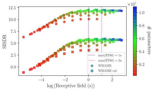
((a)) Trained on WHAMR.

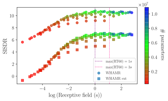
((b)) Trained on WHAMR_ext.

Figure 1: SISDR depending on logarithmic RF. Circles and squares indicate evaluation on WHAMR and WHAMR_ext test sets, respectively. Maximum RT60s of WHAMR and WHAMR_ext are shown by dashed lines. Colour scale indicates the number of model parameters.

RF and model size

Figure 1 shows the results for models trained on WHAMR (upper panel) and WHAMR_ext (lower panel) depending on the RF and model size. Note that the SISDR measure is used here, as opposed to the $\Delta$ SISDR measure, because it is later compared with SRMR in this section. In terms of model size, the SISDR performance that can be achieved by TCNs alone saturates as the number of parameters approaches 6M, for both WHAMR and WHAMR_ext when evaluated on WHAMR. For evaluation on WHAMR_ext, the SISDR performance also saturates as it approaches 6M parameters but the results for the model trained on WHAMR in Table III indicate it may benefit from the larger model size when having to dereverb larger reverberation times especially when trained only with smaller RT60s. Figure 1 further illustrates that the SISDR performance saturates before the RF reaches 1s for models trained on WHAMR, i.e. the highest occurring RT60 in WHAMR. The RF of the best performing models can be seen in Table III. The best model trained and evaluated on WHAMR in terms of SISDR has an RF of 1.02s. Analysing the same models but evaluated on WHAMR_ext the best SISDR performance is attained with an RF of 4.09s. For models trained on WHAMR_ext the optimal model evaluated on WHAMR has an RF of 1.02s and an RF of 2.04s when evaluated on WHAMR_ext. Figure 2 analyses the best performing models on each of the two datasets by their RF depending on model size (i.e. number of CB). This indicates that for larger RT60 values TCNs benefit from having a larger RF as most of the best performing models evaluated on WHAMR_ext have a larger RF than the best performing models evaluated on WHAMR.

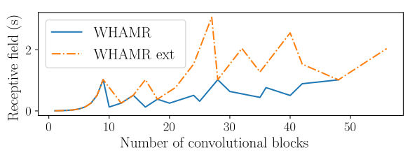
Figure 2: RFs for the best performing models in Tables I and II shown by increasing model size measured in number of CBs (one CB is 133,120 parameters). Line colour and style indicates the training and test set used.

The SISDR of the estimated signal improves even with RT60s larger than the RF as can be seen in Figure 1. This implies the network learns how to estimate masks that suppress the characteristic of reverberation, as opposed to trying to perform a blind convolution operation based on an estimated RIR representation in the network. As such, it should be possible to dereverb RIR of any RT60 value regardless of RF but Table III indicates that having an RF close to the maximum RT60 value is optimal.

SRMR vs SISDR

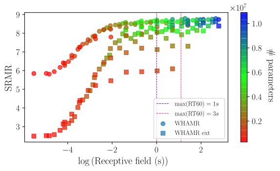
((a)) Trained on WHAMR.

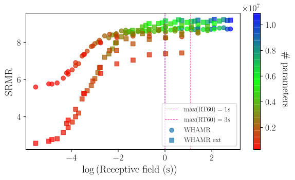
((b)) Trained on WHAMR_ext.

Figure 3: SRMR depending on logarithmic RF. Circles and squares indicate evaluation on WHAMR and WHAMR_ext test sets, respectively. Maximum RT60s of WHAMR and WHAMR_ext are shown by dashed lines. Colour scale indicates the number of model parameters.

Comparing results of SISDR (Figure 1) with SRMR (Figure 3) indicates that with sufficiently large model sizes ($\gtrsim 4$M parameters) much of the residual distortions in the signal are artifacts introduced by the network and not reverberation itself. This also indicates that the larger the reverberation time, the more residual distortions are present in the estimate clean speech signal. Audibly, the distortions present in RT60s $\lesssim 1$ were not particularly noticeable however as the RT60 approaches 3s they become more noticeable as informal listening tests showed. The performance of SRMR also saturates slightly earlier than that of SISDR similarly implying that some of the gain from increasing the model size has more correlation to reducing artefact distortions in $\hat{s}[i]$ than any residual reverberant effects. This is an argument in favour of using the SISDR function over a pure reverberation based measure like SRMR as the loss function because SRMR is more agnostic to general distortions in the signal.

Improvement on WHAMR vs WHAMR_ext

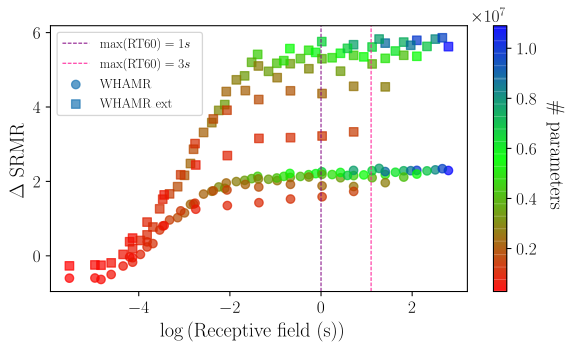
Figure 4: $\Delta$ SRMR for model trained on WHAMR depending on logarithmic RF. Circles and squares indicate evaluation on WHAMR and WHAMR_ext test sets, respectively. Maximum RT60s of WHAMR and WHAMR_ext are shown by dashed lines. Colour scale indicates the number of model parameters.

The $\Delta$ SRMR results in Figure 4 demonstrate that greater reverberation improvement can be attained on the more reverberant WHAMR_ext dataset but that larger model sizes ($\gtrsim 4$M parameters) are required to fully capitalize on this. Also for both WHAMR_ext evaluation there is much broader distribution of values as the receptive field increases. This is related to the $R$ variable in the TCN, in other words using a deeper network leads to a more significant improvement when evaluating SRMR improvement on larger RT60s.

VI Conclusion

In this paper TCNs were analysed for their application in dereverberation tasks. It was found that for smaller models more emphasis should be put on widening the RF of the network than using more layers in a network. The model performance in both SISDR and SRMR starts to saturate around a model size of $4$M parameters. It was shown that the for larger RT60 values there is strong evidence that having a wider receptive field is important for achieving optimal performance. This is especially true when the model is trained on smaller RT60s. It was found that SRMR performance was fairly agnostic to the variation in RT60 values but SISDR performance was significantly impacted. This indicates that much of the distortion remaining in the signal maybe modelling errors as opposed to reverberant effects.

References

- [1] P. A. Naylor and N. D. Gaubitch, Speech Dereverberation, 1st ed. Springer Publishing, 2010.
- [2] R. Haeb-Umbach, J. Heymann, L. Drude, S. Watanabe, M. Delcroix, and T. Nakatani, “Far-Field Automatic Speech Recognition,” Proceedings of the IEEE, vol. 109, no. 2, pp. 124–148, 2021.
- [3] T. Hain, L. Burget, J. Dines, G. Garau, M. Karafiat, M. Lincoln, J. Vepa, and V. Wan, “The AMI Meeting Transcription System: Progress and Performance,” in Proceedings of the Third International Conference on Machine Learning for Multimodal Interaction, ser. MLMI’06. Berlin, Heidelberg: Springer-Verlag, 2006, p. 419–431.
- [4] B. Cauchi, I. Kodrasi, R. Rehr, S. Gerlach, A. Jukic, T. Gerkmann, S. Doclo, and S. Goetze, “Combination of MVDR beamforming and single-channel spectral processing for enhancing noisy and reverberant speech,” EURASIP Journal on Advances in Signal Processing, vol. 2015, no. 1, 2015.
- [5] A. Oppenheim, R. Schafer, and T. Stockham, “Nonlinear filtering of multiplied and convolved signals,” IEEE Transactions on Audio and Electroacoustics, vol. 16, no. 3, pp. 437–466, 1968.
- [6] E. A. P. Habets, “Single- and multi-microphone speech dereverberation using spectral enhancement,” 2007.
- [7] S. Park, Y. Jeong, M. S. Kim, and H. S. Kim, “Linear prediction-based dereverberation with very deep convolutional neural networks for reverberant speech recognition,” in ICEIC 2018, vol. 2018-January. Institute of Electrical and Electronics Engineers Inc., April 2018, pp. 1–2.
- [8] J. Zhang, C. Zorila, R. Doddipatla, and J. Barker, “On end-to-end multi-channel time domain speech separation in reverberant environments,” ICASSP 2020, pp. 6389–6393, May 2020.
- [9] A. Purushothaman, A. Sreeram, R. Kumar, and S. Ganapathy, “Deep learning based dereverberation of temporal envelopes for robust speech recognition,” in Interspeech 2020, October 2020.
- [10] K. Kinoshita, M. Delcroix, H. Kwon, T. Mori, and T. Nakatani, “Neural network-based spectrum estimation for online WPE dereverberation,” 2017.
- [11] Y. Zhao, D. Wang, B. Xu, and T. Zhang, “Monaural speech dereverberation using temporal convolutional networks with self attention,” IEEE/ACM Transactions on Audio, Speech, and Language Processing, vol. 28, pp. 1598–1607, 2020.
- [12] Y. Luo and N. Mesgarani, “TasNet: Time-domain audio separation network for real-time, single-channel speech separation,” in ICASSP 2018, 2018, pp. 696–700.
- [13] Y. Luo and N. Mesgarani, “Real-time single-channel dereverberation and separation with time-domain audio separation network,” Interspeech 2018, 2018.
- [14] Y. Luo and N. Mesgarani, “Conv-TasNet: Surpassing ideal time–frequency magnitude masking for speech separation,” IEEE/ACM Transactions on Audio, Speech, and Language Processing, vol. 27, no. 8, pp. 1256–1266, 2019.
- [15] C. Lea, R. Vidal, A. Reiter, and G. D. Hager, “Temporal convolutional networks: A unified approach to action segmentation,” in Computer Vision – ECCV 2016 Workshops, G. Hua and H. Jégou, Eds. Cham: Springer International Publishing, 2016, pp. 47–54.
- [16] M. Maciejewski, G. Wichern, and J. Le Roux, “WHAMR!: Noisy and reverberant single-channel speech separation,” in ICASSP 2020, May 2020.
- [17] L. J. Ba, J. R. Kiros, and G. E. Hinton, “Layer normalization,” 2016, arXiv:2106.04624.
- [18] J. L. Roux, S. Wisdom, H. Erdogan, and J. R. Hershey, “SDR – half-baked or well done?” in ICASSP 2019, May 2019, pp. 626–630.
- [19] R. Scheibler, E. Bezzam, and I. Dokmanic, “Pyroomacoustics: A python package for audio room simulation and array processing algorithms,” ICASSP 2018, April 2018.
- [20] M. Ravanelli, T. Parcollet, P. Plantinga, A. Rouhe, S. Cornell, L. Lugosch, C. Subakan, N. Dawalatabad, A. Heba, J. Zhong, J.-C. Chou, S.-L. Yeh, S.-W. Fu, C.-F. Liao, E. Rastorgueva, F. Grondin, W. Aris, H. Na, Y. Gao, R. D. Mori, and Y. Bengio, “SpeechBrain: A general-purpose speech toolkit,” 2021, arXiv:2106.04624.
- [21] S. Goetze, A. Warzybok, I. Kodrasi, J. O. Jungmann, B. Cauchi, J. Rennies, E. A. P. Habets, A. Mertins, T. Gerkmann, S. Doclo, and B. Kollmeier, “A study on speech quality and speech intelligibility measures for quality assessment of single-channel dereverberation algorithms,” in IWAENC 2014, Antibes, France, 2014, pp. 233–237.
- [22] A. Rix, J. Beerends, M. Hollier, and A. Hekstra, “Perceptual evaluation of speech quality (PESQ)-a new method for speech quality assessment of telephone networks and codecs,” in ICASSP 2001, vol. 2, May 2001, pp. 749–752 vol.2.
- [23] J. Jensen and C. H. Taal, “An algorithm for predicting the intelligibility of speech masked by modulated noise maskers,” IEEE/ACM Transactions on Audio, Speech, and Language Processing, vol. 24, no. 11, pp. 2009–2022, 2016.
- [24] J. F. Santos, M. Senoussaoui, and T. H. Falk, “An improved non-intrusive intelligibility metric for noisy and reverberant speech,” in IWAENC 2014, September 2014, pp. 55–59.