Bayesian Integrals on Toric Varieties

Abstract

We explore the positive geometry of statistical models in the setting of toric varieties. Our focus lies on models for discrete data that are parameterized in terms of Cox coordinates. We develop a geometric theory for computations in Bayesian statistics, such as evaluating marginal likelihood integrals and sampling from posterior distributions. These are based on a tropical sampling method for evaluating Feynman integrals in physics. We here extend that method from projective spaces to arbitrary toric varieties.

14M25, 62F15 (primary), 65D30 (secondary)

1 Introduction

Every projective toric variety $X$ is a positive geometry [1]. Its canonical differential form $\Omega_{X}$ has poles on the toric boundary, and it encodes probability measures on the positive part $X_{>0}.$ Our aim is to develop the geometry of Bayesian statistics in this toric setting. We introduce parametric statistical models by mapping $X_{>0}$ into a probability simplex $\Delta_{m}.$ The probabilities are written in Cox coordinates on $X.$ We shall use the canonical measure on $X_{>0}$ for marginal likelihood integrals and for sampling from the posterior distribution.

We begin with an example for the product of three projective lines $X=\mathbb{P}^{1}\times\mathbb{P}^{1}\times\mathbb{P}^{1}.$ This toric threefold has six Cox coordinates $x_{0},x_{1},\,s_{0},s_{1},\,t_{0},t_{1}.$ Each letter refers to homogeneous coordinates on one of the three lines $\mathbb{P}^{1}.$ We consider the model $X_{>0}\rightarrow\Delta_{m}$ parameterized by

(1) $$p_{\ell}\,\,=\,\,\binom{m}{\ell}\frac{x_{0}}{x_{0}+x_{1}}\frac{s_{0}^{\ell}s_{1}^{m-\ell}}{(s_{0}+s_{1})^{m}}\,+\,\binom{m}{\ell}\frac{x_{1}}{x_{0}+x_{1}}\frac{t_{0}^{\ell}t_{1}^{m-{\ell}}}{(t_{0}+t_{1})^{m}}\qquad\text{for}\quad\ell=0,1,\ldots,m.$$

These expressions are rational functions on $X,$ positive on $X_{>0},$ and their sum equals $1.$ This is the conditional independence model for $m$ binary random variables with $1$ binary hidden state. Algebraically, it represents symmetric $2{\times}2{\times}\cdots{\times}2$ tensors of nonnegative rank $2.$

For an intuitive understanding, imagine a gambler who has three biased coins, one in each hand, and one more to decide which hand to use. The latter coin has probabilities $x_{0}$ and $x_{1}$ for tails and heads, and this decides whether the left hand coin (with bias $s_{0},s_{1}$) or the right hand coin (with bias $t_{0},t_{1}$) is to be used. The gambler performs $m$ coin tosses with the chosen hand and records the number of heads. The probability of observing $\ell$ heads equals $p_{\ell}.$ A more familiar formula for this event arises by dehomogenizing via $x_{1}=x,\,x_{0}=1-x,$ etc:

(2) $$p_{\ell}\,\,=\,\,\binom{m}{\ell}\left[(1-x)(1-s)^{\ell}s^{m-\ell}\,+\,x(1-t)^{\ell}t^{m-\ell}\,\right]\qquad{\rm for}\quad\ell=0,1,\ldots,m.$$

As is customary in toric geometry, we identify the positive variety $X_{>0}$ with the open cube $(0,1)^{3},$ which is the space of dehomogenized parameters $(x,s,t).$ At first glance, the passage from (2) to (1) does not change much. It is a reparameterization of the model in $\Delta_{m}=\mathbb{P}^{m}_{>0},$ which comprises positive Hankel matrices that are semidefinite and have rank $\leq 2.$ For instance, for $m=4$ coin tosses, these are the $3\times 3$ Hankel matrices shown in [8, Section 1]:

$$\begin{pmatrix}12p_{0}&3p_{1}&2p_{2}\\ 3p_{1}&2p_{2}&3p_{3}\\ 2p_{2}&3p_{3}&12p_{4}\end{pmatrix}\,\,=\,\,\frac{12}{x_{0}+x_{1}}\begin{pmatrix}s_{1}^{2}&t_{1}^{2}\\ s_{0}s_{1}&t_{0}t_{1}\\ s_{0}^{2}&t_{0}^{2}\end{pmatrix}\!\!\begin{pmatrix}\frac{x_{0}}{(s_{0}+s_{1})^{4}}\!\!&0\!\!\vskip 3.0pt plus 1.0pt minus 1.0pt\\ \!\!0&\!\!\frac{x_{1}}{(t_{0}+t_{1})^{4}}\end{pmatrix}\!\!\begin{pmatrix}s_{1}^{2}&s_{0}s_{1}&s_{0}^{2}\\ t_{1}^{2}&t_{0}t_{1}&t_{0}^{2}\end{pmatrix}.$$

The key insight for what follows is that our toric $3$-fold $X$ has a canonical $3$-form

(3) $$\Omega_{X}\,=\,\sum_{i=0}^{1}\sum_{j=0}^{1}\sum_{k=0}^{1}\,(-1)^{i+j+k}\,\frac{{\rm d}x_{i}}{x_{i}}\wedge\frac{{\rm d}s_{j}}{s_{j}}\wedge\frac{{\rm d}t_{k}}{t_{k}}.$$

This gives $(X,X_{>0})$ the structure of a positive geometry in the sense of [1]. The associated representations of prior distributions on the parameter space $X_{>0}$ offer novel tools for Bayesian inference. For instance, suppose our prior belief about the parameters $(x,s,t)$ in the coin model (2) is the uniform distribution on the cube $[0,1]^{3}.$ Its pullback to $X$ equals

(4) $$\Omega^{\rm unif}_{X}\,\,=\,\,\frac{x_{0}x_{1}s_{0}s_{1}t_{0}t_{1}}{(x_{0}+x_{1})^{2}(s_{0}+s_{1})^{2}(t_{0}+t_{1})^{2}}\,\Omega_{X}.$$

Statistics is about data. If our gambler performs the experiment $U$ times, and $\ell$ heads were observed $u_{\ell}$ times, then $\frac{1}{U}(u_{0},u_{1},\ldots,u_{m})\in\Delta_{m}$ is the empirical distribution. The likelihood function is a rational function on the toric variety $X,$ namely $L_{u}=p_{0}^{u_{0}}p_{1}^{u_{1}}\cdots p_{m}^{u_{m}}.$ The posterior distribution is the product of this function times the prior distribution on $X_{>0}.$ For the prior that is uniform on $[0,1]^{3}$ we take (4). The marginal likelihood integral equals

(5) $$\int_{X_{>0}}p_{0}^{u_{0}}p_{1}^{u_{1}}\cdots p_{m}^{u_{m}}\,\Omega^{\rm unif}_{X}.$$

Two important tasks in Bayesian statistics [7] are evaluating the integral (5) and sampling from the posterior distribution. See [10] and [15, Section 5.5] for points of entry from an algebraic perspective. In this paper, we explore these tasks using toric and tropical geometry.

We shall study our statistical problem in the following algebraic framework. Let $f$ and $g$ be homogeneous polynomials of the same degree in the Cox coordinates on an $n$-dimensional toric variety $X.$ We assume that all coefficients in $f$ and $g$ are positive real numbers, so the rational function $f/g$ has no zeros or poles on $X_{>0}.$ The integral of the $n$-form $\,(f/g)\Omega_{X}\,$ over the positive toric variety $X_{>0}$ is a positive real number, or it diverges. Our aim is to compute this number numerically. We focus on integrals of interest in Bayesian statistics.

The main contribution of this article is a geometric theory of Monte Carlo sampling, based on the positive geometry $(X,X_{>0}).$ A central role is played by the canonical form $\Omega_{X}.$ The approach was first introduced in [2] for Feynman integrals on projective space $X=\mathbb{P}^{n}.$

Our presentation is organized as follows. Section 2 reviews the quotient construction of a toric variety $X$ from its Cox ring. The canonical form $\Omega_{X}$ is defined in (10). We introduce integrals of the form $\int_{X_{>0}}(f/g)\Omega_{X},$ and we present a convergence criterion in Theorem 2.5.

In Section 3, we replace the rational function $f/g$ in the integrand by its tropicalization. The resulting piecewise monomial structure divides the positive toric variety $X_{>0}$ into sectors. Theorem 3.11 gives a formula for integrating over each sector, against the tropical probability distribution on $X_{>0}.$ 1 offers a method for sampling from that distribution. Although we here focus on its use in Bayesian statistics, we stress that the method of replacing densities by their tropical approximation is not custom-tailored for Bayesian purposes; the idea is applicable and might be beneficial more widely in statistics.

In Section 4, we develop a tropical approximation scheme for the classical integral$\,\int_{X_{>0}}(f/g)\Omega_{X}.$ We apply rejection sampling to draw from the density induced by $f/g$ on $X_{>0}$ with its canonical form $\Omega_{X}.$ The runtime is analyzed in terms of the acceptance rate.

Section 5 is devoted to discrete statistical models whose parameter space is a simple polytope $P.$ Familiar instances are linear models, toric models, and their mixtures [15]. We show how to pull back Bayesian priors from $P$ to $X_{>0}$ via the moment map. The push-forward of $\Omega_{X}$ to $P$ gives rise to the Wachspress model whose states are the vertices of $P.$ The section concludes with a combinatorial analysis of the coin model in Equation (1).

In Section 6, we apply tropical integration and tropical sampling to data analysis in the Bayesian setting. We focus on the statistical models from Section 5, but now lifted from $P$ to $X_{>0}.$ We present algorithms, along with their implementation, for computing marginal likelihood integrals. Sampling from the posterior distribution is also discussed. Our software and other supplementary material for this article is available at the repository website MathRepo [5] of MPI MiS via the link https://mathrepo.mis.mpg.de/BayesianIntegrals$\,.$

2 Toric Varieties and their Canonical Forms

We review the set-up of toric geometry, leading up to the integrals studied in this paper. For complete details on toric varieties we refer to the textbook [4] and to the notes [17]. Let $T$ be an $n$-dimensional complex algebraic torus with character lattice $M$ and co-character lattice $N=\rm Hom_{\mathbb{Z}}(M,\mathbb{Z}).$ Fixing an isomorphism $T\simeq(\mathbb{C}^{*})^{n}$ corresponds to identifying $M\simeq\mathbb{Z}^{n}$ and $N\simeq\mathbb{Z}^{n}.$ We write $\chi^{a}$ for the character in $M$ corresponding to the lattice point $a\in\mathbb{Z}^{n}$ and $\lambda^{v}$ for the co-character in $N$ corresponding to $v\in\mathbb{Z}^{n}.$ The pairing $\langle\cdot,\cdot\rangle:N\times M\rightarrow\mathbb{Z}$ is given by $\langle\lambda^{v},\chi^{a}\rangle=\chi^{a}\circ\lambda^{v}\in\rm Hom_{\mathbb{Z}}(\mathbb{C}^{*},\mathbb{C}^{*})\simeq\mathbb{Z}.$ In coordinates, this is the dot product $\langle v,a\rangle=v\cdot a.$

Fix a complete fan $\Sigma$ in $\mathbb{R}^{n}=N\otimes_{\mathbb{Z}}\mathbb{R}.$ The $n$-dimensional toric variety $X=X_{\Sigma}\supset T$ is normal and complete. Write $\Sigma(d)$ for the set of cones of dimension $d$ in $\Sigma,$ and $k=|\Sigma(1)|$ for the number of rays of $\Sigma.$ Each ray $\rho\in\Sigma(1)$ has a primitive ray generator $v_{\rho}\in\mathbb{Z}^{n},$ satisfying $\rho\cap\mathbb{Z}^{n}=\mathbb{N}\cdot\,v_{\rho}.$ We collect the rays in the columns of the $n\times k$ matrix $V=[v_{1}\,v_{2}~{}\cdots~{}v_{k}].$ This matrix has more columns than rows, i.e., $k>n$, since $\Sigma$ is complete.

The free group of torus-invariant Weil divisors on $X$ is $\text{Div}_{T}(X)=\bigoplus_{\rho}\mathbb{Z}\cdot D_{\rho}\simeq\mathbb{Z}^{k}.$ A character $\chi^{a}\in M$ extends to a rational function on $X$ with divisor $\text{div}(\chi^{a})=\sum_{\rho}\langle v_{i},a\rangle D_{\rho}.$ The transpose matrix $V^{\top},$ viewed as a map of lattices $M\rightarrow\text{Div}_{T}(X)\simeq\mathbb{Z}^{k},$ sends a character to its divisor. Two torus-invariant divisors $D_{1},D_{2}\in\text{Div}_{T}(X)$ are linearly equivalent if and only if $D_{1}-D_{2}=\text{div}(\chi^{a})$ for some character $\chi^{a}.$ Equivalently, there is an exact sequence

(6) $$0\,\longrightarrow\,M\overset{V^{\top}}{\longrightarrow}\mathbb{Z}^{k}\,\longrightarrow\,\text{Cl}(X)\,\longrightarrow\,0.$$

The cokernel $\text{Cl}(X)=\mathbb{Z}^{k}/\mathrm{im}V^{\top}$ is the divisor class group of $X.$ The Picard group $\text{Pic}(X)\subseteq\text{Cl}(X)$ is the subgroup of Cartier divisors modulo linear equivalence. Applying the functor $\rm Hom_{\mathbb{Z}}(-,\mathbb{C}^{*})$ to (6), we obtain the following exact sequence of multiplicative abelian groups:

(7) $$1\,\longrightarrow\,G\,\longrightarrow\,(\mathbb{C}^{*})^{k}\,\longrightarrow\,(\mathbb{C}^{*})^{n}\,\longrightarrow\,1.$$

The group $G=\rm Hom_{\mathbb{Z}}(\text{Cl}(X),\mathbb{C}^{*})$ is reductive: it is a quasi-torus of dimension $k-n.$

We will now recall the definition of the Cox ring of $X$. Consider the polynomial ring $S=\mathbb{C}[x_{1},\ldots,x_{k}],$ with one variable $x_{\rho}$ for each divisor $D_{\rho},$ $\rho\in\Sigma(1).$ The sequence (6) defines a grading of $S$ by the group ${\rm Cl}(X),$ and the sequence (7) gives the associated quasi-torus action by $G$ on the affine space ${\rm Spec}(S)=\mathbb{C}^{k}.$ The grading is as follows:

$$S\,\,=\bigoplus_{\gamma\in\text{Cl}(X)}\!S_{\gamma},\qquad\text{where}\qquad S_{\gamma}\,\,=\!\!\bigoplus_{a\,:\,V^{\top}a+c\geq 0}\!\!\mathbb{C}\cdot\,x^{V^{\top}a\,+\,c}.$$

The vector $c\in\mathbb{Z}^{k}$ is fixed. It represents any divisor $D_{c}=\sum_{\rho}c_{\rho}D_{\rho}$ such that $[D_{c}]=\gamma.$ The sum on the right is over all $a\in M$ such that the integer vector $V^{\top}a+c$ is nonnegative.

The toric variety $X$ can be realized as a quotient $(\mathbb{C}^{k}\backslash\mathcal{V}(B))/\!/G.$ The irrelevant ideal $B\triangleleft S$ is generated by the squarefree monomials $x^{\hat{\sigma}}=\prod_{\rho\notin\sigma}x_{\rho}$ representing maximal cones, i.e.,

$$B\,\,=\,\,\langle\,x^{\hat{\sigma}}~{}|~{}\sigma\in\Sigma(n)\,\rangle.$$

The map $(\mathbb{C}^{*})^{k}\rightarrow(\mathbb{C}^{*})^{n}$ in (7) is constant on $G$-orbits. It is the restriction of the map $\pi:\mathbb{C}^{k}\backslash\mathcal{V}(B)\rightarrow X$ which presents $X$ as the quotient above. The notation $/\!/$ indicates that this is generally not a geometric quotient. However, it is if $\Sigma$ is a simplicial fan. Under this extra assumption, we write $X=(\mathbb{C}^{k}\backslash\mathcal{V}(B))/G$ and there is a one-to-one correspondence

$$\{\text{$G$-orbits in $\mathbb{C}^{k}\backslash\mathcal{V}(B)$}\}\,\,\stackrel{{\scriptstyle 1:1}}{{\longleftrightarrow}}\,\,\{\text{points in $X$}\}.$$

The polynomial ring $S$, with its ${\rm Cl}(X)$-grading and irrelevant ideal $B$, is the Cox ring of $X.$

The zero locus in $\mathbb{C}^{k}$ of a homogeneous polynomial $f\in S$ is stable under the $G$-action. Hence, the zero locus of $f$ in $X$ is well-defined. In fact, homogeneous ideals of $S$ define subschemes of $X,$ and all subschemes arise in this way. If $X$ is smooth, then the subschemes of $X$ are in one-to-one correspondence with the $B$-saturated homogeneous ideals of $S.$

If $f,g\in S$ are homogeneous of the same degree and $g\neq 0$, the quotient $f/g$ gives a rational function on $X$, defined on the open subset $\pi\left((\mathbb{C}^{*})^{k}\setminus({\cal V}(B)\cup{\cal V}(g))\right)$ via $(f/g)(p)=f(x)/g(x)$ where $x$ is any point in the $G$-orbit $\pi^{-1}(p)$. In the rest of the paper, we will use homogeneous rational functions of degree $0$ in the fraction field of $S$ to denote the corresponding rational function on $X$. Similarly, meromorphic differential forms on $X$ can be represented by rational functions in Cox coordinates, as in (3) for $X=\mathbb{P}^{1}\times\mathbb{P}^{1}\times\mathbb{P}^{1}$. See also Remark 2.3.

The material above may look overly formal to a novice. Yet, toric varieties $X$ and their Cox coordinates $x_{1},\ldots,x_{k}$ are practical tools for applications, e.g., in the numerical solution of polynomial equations [16]. The present paper extends the utility of the abstract setting to numerical computing at the interface of statistics and physics [2, 14]. In applications, the toric variety $X$ is usually projective, i.e., $\Sigma$ is the normal fan of a lattice polytope in $\mathbb{R}^{n}.$

Example 2.1 (3-cube).

Let $n=3,$ $k=6$ and $\Sigma$ the fan given by the eight orthants in $\mathbb{R}^{3}.$ Then $X=\mathbb{P}^{1}\times\mathbb{P}^{1}\times\mathbb{P}^{1},$ with Cox ring $S=\mathbb{C}[x_{0},x_{1},s_{0},s_{1},t_{0},t_{1}],$ graded by ${\rm Cl}(X)=\mathbb{Z}^{3}.$ The irrelevant ideal is $\,B=\langle x_{0},x_{1}\rangle\,\cap\,\langle s_{0},s_{1}\rangle\,\cap\,\langle t_{0},t_{1}\rangle\,=\,\langle x_{0}s_{0}t_{0},x_{0}s_{0}t_{1},\ldots,x_{1}s_{1}t_{1}\rangle.$ We represent $X$ as the quotient of $\mathbb{C}^{6}\backslash\mathcal{V}(B)$ modulo the action $G=(\mathbb{C}^{*})^{3},$ as in the Introduction. See [11, Example 6.2.7 (2)] for a detailed study of this example and its tropicalization.

Figure 1: This pentagon specifies the projective toric surface in Example 2.2.

Example 2.2 (Pentagon).

Fix $n=2,$ $k=5,$ and the polygon in Figure 1. The rays of its normal fan $\Sigma$ are the inner normals to the edges. We write their generators in the matrix

(8) $$V\,\,=\,\,\begin{pmatrix}\,\,1&\phantom{-}1&-1&-1&\,0\,\,\\ \,\,0&-1&-1&\phantom{-}1&\,1\,\,\end{pmatrix}.$$

We have $G\simeq(\mathbb{C}^{*})^{3},$ since ${\rm Cl}(X)=\mathbb{Z}^{5}/{\rm im}\,V^{\top}$ is isomorphic to $\mathbb{Z}^{3}.$ The irrelevant ideal is

$$B=\langle x_{1}x_{2}x_{3},x_{2}x_{3}x_{4},x_{3}x_{4}x_{5},x_{4}x_{5}x_{1},x_{5}x_{1}x_{2}\rangle\,\,\triangleleft\,\,S=\mathbb{C}[x_{1},x_{2},x_{3},x_{4},x_{5}].$$

The map $(x_{1},\ldots,x_{5})\!\mapsto\!\!\!\;(x_{1}x_{2}x_{3}^{-1}x_{4}^{-1}\!,x_{2}^{-1}x_{3}^{-1}x_{4}x_{5})$ represents $X$ as the quotient $(\mathbb{C}^{5}\setminus\mathcal{V}(B))/G.$ We find it convenient to write the image of $V^{\top}$ in $\mathbb{Z}^{5}$ as the kernel of another matrix, e.g.,

(9) $$W\,\,=\,\,\begin{pmatrix}0&1&0&1&0\\ 1&0&1&0&1\\ 2&0&1&1&0\\ \end{pmatrix}.$$

The $\mathbb{Z}^{3}$-grading of $S$ sends $x_{i}$ to the $i$-th column of $W.$ The $G$-action on $\mathbb{C}^{5}$ is

$$x_{1}\,\mapsto\,t_{2}t_{3}^{2}\,x_{1},\,\,x_{2}\,\mapsto\,t_{1}x_{2},\,\,x_{3}\,\mapsto\,t_{2}t_{3}x_{3},\,\,x_{4}\,\mapsto\,t_{1}t_{3}x_{4},\,\,x_{5}\,\mapsto\,t_{2}x_{5}.$$

If $c\in\mathbb{Z}^{5}$ then $\gamma=Wc\in\mathbb{Z}^{3}$ represents the class $[D_{c}]\in{\rm Cl}(X)$ of the divisor $D_{c}$ on $X$.

The positive orthant $\mathbb{R}^{k}_{>0}$ is disjoint from $\mathcal{V}(B)$ since $B$ is a monomial ideal. We can restrict the quotient map $\mathbb{C}^{k}\backslash\mathcal{V}(B)\rightarrow X$ to $\mathbb{R}^{k}_{>0}.$ The image of this restriction is the positive part $X_{>0}$ of the toric variety $X.$ The Euclidean closure of $X_{>0}$ in $X$ is denoted $X_{\geq 0}.$ If $X$ is projective with polytope $P$ then the moment map gives a homeomorphism from $X_{>0}$ onto $P^{\circ}.$

Motivated by statistics (see Equation (5)), we wish to integrate meromorphic $n$-forms with poles outside $X_{>0}$ over the nonnegative part $X_{\geq 0}.$ We here describe an explicit representation of such forms via the Cox ring $S.$ For any $n$-element subset $I\subset\Sigma(1),$ let $\det(V_{I})$ denote the minor of $V$ indexed by $I.$ We define a meromorphic $n$-form on $\mathbb{C}^{k}$ as follows:

(10) $$\Omega_{X}\,\,\,=\,\,\sum_{\begin{subarray}{c}I\subset\Sigma(1),\,|I|=n\end{subarray}}\det(V_{I})\,\bigwedge_{\rho\in I}\frac{{\rm d}x_{\rho}}{x_{\rho}}.$$

This is the canonical form of the pair $(X,X_{\geq 0}),$ viewed as a positive geometry, as explained by Arkani-Hamed, Bai, and Lam in [1, Sect. 5.6.2]. The canonical form $\Omega_{X}$ is the pullback under the quotient map $\pi$ of the $T$-invariant $n$-form $\bigwedge_{j=1}^{n}\frac{{\rm d}t_{j}}{t_{j}}\in\Omega_{T}^{n}(T),$ where $t_{j}=\chi^{e_{j}}$ are coordinates on $T.$ This follows from [4, Cor. 8.2.8] by observing that $\pi^{*}(t_{j})=\prod_{i=1}^{k}x_{\rho}^{\langle v_{i},e_{j}\rangle}.$ By homogeneity, $\Omega_{X}$ can be viewed as a meromorphic form on $X.$ We will use $\Omega_{X}$ to denote this form on $\mathbb{C}^{k},$ on $X,$ as well as its restriction to $X_{>0}$ without mentioning the respective transition.

After scaling by a rational function, the canonical form $\Omega_{X}$ defines a probability measure on $X_{>0}.$ Given a rational function $f/g$ on $X$, we are interested in the definite integral of the differential form $(f/g)\,\Omega_{X}$ over the positive toric variety $X_{>0}$. In symbols, this equals

(11) $$\mathcal{I}\,\,\,=\,\,\,\int_{X_{>0}}\frac{f}{g}\,\Omega_{X}.$$

The integrals $\mathcal{I}$ appear as Feynman integrals in physics. The article [2] introduces tropical sampling for Feynman integrals over the projective space $X=\mathbb{P}^{n}.$ The present paper generalizes that approach to the setting where $X$ can be any toric variety.

Remark 2.3.

The canonical form $\Omega_{X}$ of a toric variety $X$ is closely related to the canonical sheaf $\omega_{X}.$ Indeed, by the discussion following [4, Corollary 8.2.8], $\omega_{X}$ is the sheaf of the cyclic graded $S$-module generated by the $n$-form $\left(\prod_{i=1}^{k}x_{i}\right)\Omega_{X}.$ See also [3, Proposition 2.1].

We next explain how to understand and evaluate the integral (11). Let $\gamma=\deg(f)=\deg(g)\in{\rm Cl}(X)$ be the class of the divisor $D_{c}.$ The canonical isomorphism

$$S_{\gamma}\,\,=\!\!\bigoplus_{a\,:\,V^{\top}a+c\,\geq 0}\!\!\mathbb{C}\cdot\,x^{V^{\top}a\,+\,c}\,\,\simeq\bigoplus_{a\,:\,V^{\top}a+c\,\geq 0}\mathbb{C}\cdot\,t^{a}$$

represents dehomogenization. It sends $f$ and $g$ to Laurent polynomials $\hat{f}$ and $\hat{g},$ respectively.

This is compatible with the quotient map $\pi:\mathbb{C}^{k}\backslash{\cal V}(B)\rightarrow X$ in the following way. The map of tori $\pi_{|(\mathbb{C}^{*})^{k}}:(\mathbb{C}^{*})^{k}\rightarrow T\subset X$ realizes the torus of $X$ as a geometric quotient $T\simeq(\mathbb{C}^{*})^{k}/G.$ Further restricting to the positive part gives $T_{>0}\simeq X_{>0}.$ Let $\phi:X_{>0}\rightarrow T_{>0}$ denote this diffeomorphism. In Cox coordinates, $\phi$ is the monomial map given by the rows of $V,$ see Example 2.2. One checks easily that the functions $(f/g):X_{>0}\rightarrow\mathbb{C}$ and $(\hat{f}/\hat{g}):T_{>0}\rightarrow\mathbb{C}$ satisfy $(f/g)=(\hat{f}/\hat{g})\circ\phi.$ Moreover, $\Omega_{X}$ restricted to its dense torus is the form $\pi^{*}\left(\bigwedge_{j=1}^{n}\frac{{\rm d}t_{j}}{t_{j}}\right)$ which, in turn, uniquely determines $\Omega_{X}.$ Those observations imply the following proposition.

Proposition 2.4.

The integral $\mathcal{I}$ in (11) equals a more familiar integral over the positive orthant $T_{>0}=\mathbb{R}^{n}_{>0},$ namely

(12) $$\mathcal{I}\,\,\,=\,\,\,\int_{T_{>0}}\frac{\hat{f}}{\hat{g}}\,\bigwedge_{j=1}^{n}\frac{{\rm d}t_{j}}{t_{j}}.$$

We conclude Section 2 with a result on convergence. This 2.5 generalizes [2, Theorem 3].

Theorem 2.5.

Suppose that the Newton polytope of the denominator $g$ is $n$-dimensional and contains that of the numerator $f$ in its relative interior. Then the integral (11) converges.

Proof 2.6.

We use the formulation in (12). By linearity of the integral, it suffices to consider the case when $f$ is a monomial. In that special case, our integral can be viewed as the Mellin transform of the polynomial $g$. Hence the analysis by Nilsson and Passare in [12] applies here. Their result is stated for integrals over $T_{\geq 0}=\mathbb{R}^{n}_{\geq 0},$ so we can use it for (12). The convergence result then follows from [12, Theorem 1].

Remark 2.7.

The hypothesis of Theorem 2.5 will be satisfied for the Bayesian integrals that arise from our statistical models in Sections 5 and 6. An example is the integrand in (4). The Newton polytope of the denominator is the standard $3$-cube scaled by a factor of two. Its unique interior lattice point is the Newton polytope of the monomial in the numerator.

In fact, it can be proven that the hypothesis of Theorem 2.5 is also necessary for the convergence of (11) as long as the polynomials $f$ and $g$ have positive coefficients. Hence, we can expect convergent statistical integrals over ratios of such polynomials to fulfill it.

3 Tropical Sampling

Our aim is to evaluate the integral $\,\mathcal{I}\,$ in (11) and (12). To this end, we consider a tropicalized version of the integral. Following [2], we define the tropical approximation of a polynomial $f\in S=\mathbb{C}[x_{1},\ldots,x_{k}]$ to be the piecewise monomial function

$$f^{\rm tr}\colon\,\mathbb{R}_{>0}^{k}\longrightarrow\mathbb{R}_{>0},\quad x~{}\mapsto\max_{\ell\in\operatorname{supp}(f)}x^{\ell}.$$

This differs in two aspects from the textbook definition of tropicalization in [11]. First, we adopt the max-convention. Second, we use monomials $x^{\ell}$ instead of linear forms $\langle x,\ell\rangle.$ Thus $f^{\rm tr}$ is the exponential of the piecewise-linear convex function ${\rm trop}(f)$ usually derived from $f$.

If $f\in S\backslash\{0\}$ is homogeneous with positive coefficients, then the ratio $f(x)/f^{\rm tr}(x)$ is a well-defined function on $\mathbb{R}^{k}_{>0}\subset\mathbb{C}^{k}\backslash\mathcal{V}(B)$ and is constant on $G$-orbits. It induces a function $X_{>0}\rightarrow\mathbb{R}_{>0},$ which takes $x\in X_{>0}$ to $f(x^{\prime})/f^{\rm tr}(x^{\prime})$ for any $x^{\prime}\in\pi^{-1}(x).$ Employing a slight abuse of notation, the ratio $f(x)/f^{\rm tr}(x)$ also denotes that function on $X_{>0}.$

As a special case of [2, Theorems 8A and 8B], where also polynomials with negative or complex coefficients are allowed, such functions are bounded above and below:

Proposition 3.1.

Suppose that $f(x)=\sum_{\ell\in\operatorname{supp}(f)}f_{\ell}\,x^{\ell}$ has positive coefficients, and set $\,C_{1}=\min_{\ell\in\operatorname{supp}(f)}f_{\ell}\,$ and $\,C_{2}=\sum_{\ell\in\operatorname{supp}(f)}f_{\ell}.$ Then, we have

$$0\,<\,C_{1}\,\leq\,\frac{f(x)}{f^{\rm tr}(x)}\,\leq\,C_{2}\,<\,\infty\quad\text{for all $\,x\in X_{>0}$}.$$

We assume from now on that $f$ and $g$ are homogeneous polynomials in $S,$ with positive coefficients, of the same degree in ${\rm Cl}(X),$ and that the hypothesis of Theorem 2.5 is satisfied.

Corollary 3.2.

The following integral over the positive toric variety is finite:

(13) $$\mathcal{I}^{\rm tr}\,\,\,=\,\,\int_{X_{>0}}\frac{f^{\rm tr}}{g^{\rm tr}}\,\Omega_{X}.$$

Proof 3.3.

The tropical function $f^{\rm tr}/g^{\rm tr}$ is positive on $X_{>0}$ and it is bounded above by a constant times the classical function $f/g.$ This follows by applying Proposition 3.1 to both $f$ and $g.$ Since the integral over $f/g$ is finite, so is the integral over $f^{\rm tr}/g^{\rm tr}.$

The function $f^{\rm tr}/g^{\rm tr}$ is piecewise monomial on $X_{>0}.$ The pieces are the sectors to be described below. The integral of each monomial over its sector is given in Theorem 3.11. The value of $\mathcal{I}^{\rm tr}$ is the sum (18) of the sector integrals. Here is an illustration:

Example 3.4 (Classical integral versus tropical integral).

We fix the projective line $X=\mathbb{P}^{1}$ with coordinates $(x_{0}:x_{1}).$ The following binary cubics satisfy our convergence hypotheses:

$$f\,=\,x_{0}^{2}x_{1}\quad{\rm and}\quad g\,=\,(x_{0}+x_{1})(x_{0}+3x_{1})(5x_{0}+x_{1}).$$

The corresponding tropical polynomial functions on the line segment $X_{\geq 0}=\mathbb{P}^{1}_{\geq 0}$ are

$$f^{\rm tr}\,=\,f=x_{0}^{2}x_{1}\quad{\rm and}\quad g^{\rm tr}\,=\,\begin{cases}\,x_{0}^{3}&{\rm if}\,\,x_{0}\geq x_{1},\\ \,x_{1}^{3}&{\rm if}\,\,x_{0}\leq x_{1}.\end{cases}$$

The classical integral (11) equals $\frac{1}{56}(6\,{\rm ln}(3)-{\rm ln}(5))=0.088968....$ We find this on either chart $\{x_{0}=1\}$ or $\{x_{1}=1\}.$ The tropical integral (13) evaluates to $1+\frac{1}{2}=\frac{3}{2}.$ We integrate the two monomials in $f^{\rm tr}/g^{\rm tr}$ over the sectors $\{x_{0}\geq x_{1}\}$ and $\{x_{0}\leq x_{1}\}.$

Since the tropical integral is easier to compute, we now rewrite (11) as

(14) $$\mathcal{I}\,\,=\,\,\int_{X_{>0}}\!\frac{f}{g}\,\Omega_{X}\,\,\,=\,\,\,\mathcal{I}^{\rm tr}\cdot\int_{X_{>0}}\!\!h\,\,\mu^{\rm tr}_{f,g}\,,$$

where

$$h\,=\,\frac{f\cdot g^{\rm tr}}{g\cdot f^{\rm tr}}\quad\text{ and }\quad\mu^{\rm tr}_{f,g}\,=\,\frac{1}{\mathcal{I}^{\rm tr}}\frac{f^{\rm tr}}{g^{\rm tr}}\,\Omega_{X}.\qquad\qquad$$

The function $h$ is positive and bounded on $X_{>0},$ again by Proposition 3.1. The differential form $\mu^{\rm tr}_{f,g}$ is nonnegative on $X_{>0},$ and it integrates to $1.$ In symbols,

$$\int_{X_{>}0}\mu_{f,g}^{\text{tr}}\,\,=\,\,1.$$

Viewed statistically, the following function is a probability density on $X_{>0}$:

(15) $$d_{f,g}^{\,\text{tr}}\,\,\coloneqq\,\,\frac{1}{\mathcal{I}^{\text{tr}}}\frac{f^{\text{tr}}}{g^{\text{tr}}}.$$

This density is given in terms of $\mathcal{I}^{\text{tr}}$ and the tropical approximations of $f$ and $g.$ For brevity, we refer to $d_{f,g}^{\,\text{tr}}$ as the tropical density. In those terms, $\mu_{f,g}^{\text{tr}}=d_{f,g}^{\text{tr}}\cdot\Omega_{X}$ is a probability measure on $X_{>0}$ and the pair $(X_{>0},\mu_{f,g}^{\text{tr}})$ is a probability space. For basic terminology from probability, we refer to the textbook [13], and to the guided tours in [7, Chapter 1] and [15, Chapter 2].

If we can draw samples from the distribution defined by the tropical density, then we can use Monte Carlo integration to estimate the integral (11). Furthermore, using rejection sampling, we can also produce samples from the classical density $d_{f,g}=\frac{1}{\mathcal{I}}\,\frac{f}{g}$ on $X_{>0},$ where the value of the integral (11) plays the role of a normalization factor. We will describe these computations in the next section. They play a fundamental role in Bayesian inference. For an introduction to Bayesian statistics see [7].

In the remainder of this section, we present our tropical sampling algorithm, for sampling from the probability distribution on $X_{>0}$ that is given by the tropical density $d_{f,g}^{\,\text{tr}}.$ This algorithm was introduced in [2] for the special case of projective space $X=\mathbb{P}^{n},$ and it was successfully applied to Feynman integrals. We here extend it to other toric varieties $X.$

The Newton polytopes $\mathcal{N}(f)$ and $\mathcal{N}(g)$ of the homogeneous polynomials $f$ and $g$ live in $\mathbb{R}^{k},$ but their dimension is at most $n,$ since they lie in an affine translate of ${\rm im}_{\mathbb{R}}(V^{\top})\simeq\mathbb{R}^{n}.$ In light of Theorem 2.5, we assume that $\mathcal{N}(g)$ has the maximal dimension $n.$ We are interested in the normal fan of the $n$-dimensional polytope $\mathcal{N}(f)+\mathcal{N}(g)=\mathcal{N}(fg),$ which lies in a different affine translate of ${\rm im}_{\mathbb{R}}(V^{\top}).$ Its normal fan has the lineality space $K:={\rm ker}(V)\simeq\mathbb{R}^{k-n},$ so that fan can be seen as a pointed fan in $\mathbb{R}^{k}/\,K\simeq\mathbb{R}^{n}.$ We fix a simplicial refinement $\mathcal{F}$ of this normal fan. Each maximal cone of $\mathcal{F}$ is spanned by $n$ linearly independent vectors, and the union of these cones covers $\mathbb{R}^{k}/\,K.$ We alert the reader that there are now two different fans: $\Sigma$ is the fan of the toric variety $X,$ whereas $\mathcal{F}$ comes from our polynomials $f$ and $g.$

Example 3.5.

In the application to Feynman integrals in [2], the polynomials $f$ and $g$ are Symanzik polynomials. Their Newton polytopes are generalized permutohedra [2, Section 6]. For such integrals, we can take $\mathcal{F}$ to be the fan determined by the hyperplanes $\{x_{i}=x_{j}\}.$ The computational results in [2, Section 7.4] rely on this special combinatorial structure.

We now abbreviate $e^{y}=(e^{y_{1}},\ldots,e^{y_{k}}),$ and we define the exponential map

(16) $${\rm Exp}\,:\,\mathbb{R}^{k}/\,K\,\rightarrow\,X_{>0}\,,\quad[(y_{1},\ldots,y_{k})]\,\mapsto\,\pi(e^{y}).$$

Here $\pi:\mathbb{C}^{k}\setminus{\cal V}(B)\rightarrow X$ is the quotient map from Section 2. The map ${\rm Exp}$ is well-defined since the subspace $K$ is mapped into the image of $G$ under the homomorphism $\mathbb{R}^{k}\rightarrow(\mathbb{C}^{*})^{k},\,y\mapsto e^{y},$ cf. the exact sequences (6) and (7).

Remark 3.6.

The exponential map is an inverse to tropicalization. The coordinate-wise logarithm map $\mathbb{R}_{>0}^{k}\rightarrow\mathbb{R}^{k}$ turns the multiplicative action of $G$ into an additive action of $K.$ That is, it induces a map ${\rm Log}:X_{>0}\rightarrow\mathbb{R}^{k}/\,K.$ We refer to [11, Chapter 6] for details.

We continue to retain the hypotheses $\,{\rm dim}(\,\mathcal{N}(g)\,)=n\,$ and $\,\mathcal{N}(f)\subseteq{\rm relint}\,\mathcal{N}(g).$

Lemma 3.7.

For all nonzero elements $y\in\mathbb{R}^{k}/\,K,$ we have

(17) $$\max_{\nu\in\mathcal{N}(g)}y\cdot\nu\,-\,\max_{\nu\in\mathcal{N}(f)}y\cdot\nu\,\,>\,\,0.$$

Proof 3.8.

The left hand side of the inequality is well-defined modulo $K,$ because both Newton polytopes lie in the same affine translate of $K.$ Suppose the two maxima are attained for $\nu_{f}\in\mathcal{N}(f)$ and $\nu_{g}\in\mathcal{N}(g).$ If $y\cdot\nu_{g}\leq y\cdot\nu_{f}$ were to hold, then $\nu_{f}$ lies in both $\mathcal{N}(f)$ and the boundary of $\mathcal{N}(g).$ This contradicts our hypothesis. We therefore have $y\cdot\nu_{g}>y\cdot\nu_{f}.$

Lemma 3.9.

Fix a cone $\sigma$ in the simplicial fan $\mathcal{F}$ and consider any vertices $\nu_{f}$ and $\nu_{g}$ of the corresponding faces of the Newton polytopes $\mathcal{N}(f)$ and $\mathcal{N}(g).$ Then

$$\qquad\frac{f^{\rm tr}(x)}{g^{\rm tr}(x)}\,\,=\,\,x^{-(\nu_{g}-\nu_{f})}\quad\text{for all $\,x\in\mathbb{R}^{k}$ such that $\,\pi(x)\in{\rm Exp}(\sigma).$}$$

Proof 3.10.

By definition of the normal fan, the two functions $y\mapsto\max_{\nu\in\mathcal{N}(f)}y\cdot\nu$ and $y\mapsto\max_{\nu\in\mathcal{N}(g)}y\cdot\nu$ are linear on the cone $\sigma.$ Let $y\in\sigma$ satisfy $\operatorname{Exp}(y)=x.$ We have

$$\log f^{\rm tr}(x)\,=\,\log\max_{\ell\in\textrm{supp}(f)}x^{\ell}\,=\,\max_{\ell\in\textrm{supp}(f)}\ell\cdot y\,=\,\max_{\nu\in\mathcal{N}(f)}\nu\cdot y\,=\,\nu_{f}\cdot y.$$

Similarly, $\log g^{\rm tr}(x)\,=\,\nu_{g}\cdot y.$ Applying the exponential function yields the assertion.

To evaluate the integral (11), we use the factorization in (14). The first task is to evaluate the tropical integral $\mathcal{I}^{\rm tr}.$ Since ${\rm Exp}$ is a bijection, we use the decomposition

(18) $$\mathcal{I}^{\rm tr}\,\,=\,\,\sum_{\sigma\in\mathcal{F}(n)}\!\mathcal{I}^{\rm tr}_{\sigma}\qquad{\rm where}\qquad\mathcal{I}^{\rm tr}_{\sigma}\,\,\,=\,\,\int_{{\rm Exp}(\sigma)}\frac{f^{\rm tr}}{g^{\rm tr}}\,\Omega_{X}.$$

The positive toric variety $X_{>0}$ is partitioned into the sectors ${\rm Exp}(\sigma).$ Each tropical integral $\,\mathcal{I}^{\rm tr}_{\sigma}$ is the integral of a Laurent monomial of degree zero, namely $x^{-\delta_{\sigma}},$ where $\delta_{\sigma}=\nu_{g}-\nu_{f}.$ The integral of $x^{-\delta_{\sigma}}$ over all of $X_{>0}$ diverges, but our set-up ensures that it converges on the sector ${\rm Exp}(\sigma).$ We saw this for $X=\mathbb{P}^{1}$ in Example 3.4.

We next present a formula for the integral $\,\mathcal{I}^{\rm tr}_{\sigma}.$ We fix a matrix $W=[w_{1}\,\cdots\,w_{n}]\in\mathbb{R}^{k\times n}$ whose $n$ column vectors $w_{\ell}$ generate the simplicial cone $\sigma$ in $\mathbb{R}^{k}/K.$

Theorem 3.11.

The tropical sector integral in (18) is equal to

(19) $$\mathcal{I}^{\rm tr}_{\sigma}\,\,=\,\,\frac{\det(VW)}{\prod_{\ell=1}^{n}w_{\ell}\cdot\delta_{\sigma}}.$$

Before proving (19), we comment on its interpretation. The columns $w_{\ell}$ of $W$ are only defined up to the equivalence in $\mathbb{R}^{k}/K.$ Still, the numerator is well-defined, because $\det(VW)=\det(VW^{\prime})$ for any choices of representatives in the matrix $W^{\prime}=\left[w_{1}^{\prime}\,\cdots\,w_{n}^{\prime}\right]$ with $w_{i}^{\prime}=w_{i}+\lambda_{i}$ and $\lambda_{i}\in K=\ker V.$ As $x^{-\delta_{\sigma}}$ has degree 0, we have $\delta_{\sigma}=\nu_{g}-\nu_{f}\in{\rm im}_{\mathbb{R}}(V^{\top})=K^{\perp}.$ Thus, the denominator does not depend on the choice of representative for $w_{\ell}.$ Similarly, the lengths of the generators $w_{\ell}$ are irrelevant for the description of the cone. The quotient in (19) is invariant under rescalings of a vector $w_{\ell}\rightarrow\xi w_{\ell},$ as the multiplier $\xi,$ which factors out of the determinant, cancels between the numerator and the denominator. The sign of the numerator depends on the ordering of the vectors $w_{\ell}$ in $W$ which is arbitrary a priori. We arrange them in the matrix $W$ so that the condition $\det(VW)>0$ holds. Hence, the value of $\mathcal{I}^{\rm tr}_{\sigma}$ is an invariant of the cone $\sigma$ equipped with a positive orientation and the data $V$ and $\delta_{\sigma}.$ By Lemma 3.7, we have $w_{\ell}\cdot\delta_{\sigma}>0$ for all $\ell$ and hence $0<\mathcal{I}^{\rm tr}_{\sigma}<\infty$ for all $\sigma.$

Proof 3.12.

From Lemma 3.9 and our discussion above, we know that

$$\mathcal{I}_{\sigma}^{\rm tr}\,\,=\,\int_{{\rm Exp}(\sigma)}\!\!\!\!\!\!x^{-\delta_{\sigma}}\,\Omega_{X}.$$

We expand $\Omega_{X}$ as in (10), and we change coordinates under the exponential map:

(20) $$\mathcal{I}_{\sigma}^{\rm tr}\,\,=\,\,\int_{\sigma}e^{-y\cdot\delta_{\sigma}}\!\sum_{\begin{subarray}{c}I\subset\Sigma(1),\\ |I|=n\end{subarray}}\!\det(V_{I})\,\bigwedge_{i\in I}{\rm d}y_{i}\quad=\,\,\sum_{\begin{subarray}{c}I\subset\Sigma(1),\\ |I|=n\end{subarray}}\!\!\det(V_{I})\int_{\sigma}e^{-y\cdot\delta_{\sigma}}\bigwedge_{i\in I}{\rm d}y_{i}.$$

On the right is the integral of the exponential of a linear form over a simplicial cone. Since $\sigma$ is the image of $\mathbb{R}^{n}_{>0}$ under the linear map given by the matrix $W_{I},$ we obtain

$$\int_{\sigma}e^{-y\cdot\delta_{\sigma}}\bigwedge_{i\in I}{\rm d}y_{i}\quad=\quad\frac{{\rm det}(W_{I})}{\prod_{\ell=1}^{n}w_{\ell}\cdot\delta_{\sigma}}.$$

The Cauchy–Binet formula $\,\det(VW)=\sum_{I}\det(V_{I})\det(W_{I})\,$ now proves (19).

The next result generalizes [2, Lemma 17]. For an arbitrary kernel $\psi,$ the sector integral is transformed to the standard cube. Our proof technique is adapted from [2].

Proposition 3.13.

For any bounded function $\psi:X_{>0}\rightarrow\mathbb{R},$ we have

(21) $$\int_{{\rm Exp}(\sigma)}\!\frac{f^{\rm tr}}{g^{\rm tr}}\,\psi\,\,\Omega_{X}\quad=\quad\mathcal{I}^{\rm tr}_{\sigma}\,\cdot\,\int_{[0,1]^{n}}\!\!\psi(x^{\sigma}(q))\,{\rm d}q_{1}\wedge\cdots\wedge{\rm d}q_{n},$$

where

(22) $$x_{i}^{\sigma}(q)\,\,=\,\,\prod_{\ell=1}^{n}q_{\ell}^{-(w_{\ell})_{i}/(w_{\ell}\cdot\delta_{\sigma})}\quad{\rm for}\,\,\,i=1,2,\ldots,k.$$

In particular, the integral in (21) is finite for any cone $\sigma\in\mathcal{F}(n).$

Proof 3.14.

With the exponential map as in (20), the integral on the left equals

(23) $$\sum_{\begin{subarray}{c}I\subset\Sigma(1),\\ |I|=n\end{subarray}}\det(V_{I})\cdot\int_{\sigma}e^{-y\cdot\delta_{\sigma}}\psi({\rm Exp}(y))\,\bigwedge_{\rho\in I}{\rm d}y_{\rho}.\qquad$$

Using coordinates $\lambda$ on $\mathbb{R}^{n}_{>0},$ and writing $y_{i}=\sum_{\ell=1}^{n}\lambda_{\ell}(w_{\ell})_{i}$, the integral in (23) is

$$\qquad\qquad\det(W_{I})\cdot\int_{\mathbb{R}^{n}_{>0}}e^{-(W\lambda)\cdot\delta_{\sigma}}\psi({\rm Exp}(W\lambda))\,\prod_{\ell=1}^{n}\textrm{d}\lambda_{\ell}.$$

We now transform the integral from $\mathbb{R}^{n}_{>0}$ to the cube $[0,1]^{n}$ using the logarithm function. Namely, we apply the transformation $\lambda_{\ell}=(w_{\ell}\cdot\delta_{\sigma})^{-1}\log(q_{\ell})$ for $\ell=1,\ldots,n.$ This yields the right hand side in (21). This last step uses the fact that $w_{\ell}\cdot\delta_{\sigma}>0,$ which is known from Lemma 3.7. Together with boundedness of $\psi,$ this implies convergence.

Remark 3.15.

The formula (22) is a parameterization of each sector by a standard cube:

$$x^{\sigma}:[0,1]^{n}\rightarrow{\rm Exp}(\sigma),\quad q\mapsto x^{\sigma}(q).$$

To digest the exponent in (22), note that the $(i,\ell)$-th entry of $W$ is the $i$th entry $(w_{\ell})_{i}$ of the vector $w_{\ell},$ that $\delta_{\sigma}$ lies in $K,$ and that the row vector $\delta_{\sigma}\cdot W$ has coordinates $w_{\ell}\cdot\delta_{\sigma}.$

We use the sector decomposition of $X_{>0}$ given by the fan $\mathcal{F}$ to evaluate the integral (11). Rewriting (11) as in (14), the parameterization $\,\operatorname{Exp}:\mathbb{R}^{k}/K\rightarrow X_{>0}\,$ gives

(24) $$\int_{X_{>0}}\frac{f}{g}\,\Omega_{X}\,\,=\,\,\int_{X_{>0}}\frac{f^{\rm tr}}{g^{\rm tr}}\,\,h\,\Omega_{X}\,\,=\sum_{\sigma\in\mathcal{F}(n)}\int_{{\rm Exp}(\sigma)}\frac{f^{\rm tr}}{g^{\rm tr}}\,h\,\Omega_{X}.$$

Each integral on the right hand side is an integral over the cube by Proposition 3.13. These integrals over $[0,1]^{n}$ are suitable to be evaluated using black-box integration algorithms. We implemented this in Julia, using the package Polymake.jl (v0.6.1) for polyhedral computations; see [6, 9] and [5]. Moreover, specializing to $h=1$ in this representation of (11) gives a method for computing the normalization factor $\,\mathcal{I}^{\rm tr}=\sum_{\sigma\in\mathcal{F}(n)}\mathcal{I}^{\rm tr}_{\sigma}\,$ in Equation (14).

Remark 3.16.

The sector decomposition (24) gives an alternative proof of Theorem 2.5, with no reference to [12]. It would be interesting to undertake a more detailed study of the Mellin transform from a tropical perspective.

Proposition 3.13 also gives the desired algorithm to sample from the distribution in (14). As input we need the simplicial fan $\mathcal{F},$ where each maximal cone $\sigma$ comes with the following data: a generating set, the vector $\delta_{\sigma}$ that encodes the function $f^{\rm tr}/g^{\rm tr}$ as in Lemma 3.9, and the numbers $\mathcal{I}_{\sigma}^{\rm tr}$ in (19). Hence we also know $\mathcal{I}^{\rm tr}=\sum_{\sigma\in\mathcal{F}(n)}\mathcal{I}_{\sigma}^{\rm tr}.$

Algorithm 1 (Sampling from the tropical density $d_{f,g}^{\,\text{tr}}$).

Input: $\mathcal{F}(n),\,\delta_{\sigma},\,\mathcal{I}_{\sigma}^{\rm tr}$ and $\,\mathcal{I}^{\rm tr}.$

1. Draw an $n$-dimensional cone $\sigma$ from $\mathcal{F}(n)$ with probability $\,\mathcal{I}_{\sigma}^{\rm tr}/\mathcal{I}^{\rm tr}.$

2. Draw a sample $q$ from the unit hypercube $[0,1]^{n}$ using the uniform distribution.

3. Compute $x^{\sigma}(q)\in\operatorname{Exp}(\sigma)$ with $x^{\sigma}(q)$ as in Proposition 3.13.

Output: The element $x^{\sigma}(q)\in X_{>0},$ a sample from the probability space $(X_{>0},\mu^{\rm tr}_{f,g}).$

The vector $\delta_{\sigma}$ and the generators of $\sigma$ enter in the definition of the function $x^{\sigma}(q)$ in step 3. To show the correctness of 1, consider any bounded test function $\psi:X_{>0}\rightarrow\mathbb{R}.$ By Proposition 3.13, the expected value of the function $(\sigma,q)\mapsto\psi(x^{\sigma}(q))$ on ${\cal F}(n)\times[0,1]^{n},$ where $\sigma$ and $q$ are sampled by steps 1 and 2, is

$$\sum_{\sigma\in\mathcal{F}(n)}\frac{\mathcal{I}^{\rm tr}_{\sigma}}{\mathcal{I}^{\rm tr}}\,\int_{[0,1]^{n}}\!\psi(x^{\sigma}(q))\,{\rm d}q_{1}\wedge\cdots\wedge{\rm d}q_{n}\\ \,\,=\,\,\frac{1}{\mathcal{I}^{\rm tr}}\,\sum_{\sigma\in\mathcal{F}(n)}\int_{{\rm Exp}(\sigma)}\frac{f^{\rm tr}(x)}{g^{\rm tr}(x)}\,\psi(x)\,\,\Omega_{X}.$$

We conclude from (14) that the sum on the right is equal to the desired expectation

$$\mathbb{E}_{\mu_{f,g}^{\text{tr}}}[\psi]\,\,\,=\,\,\,\int_{X_{>0}}\!\psi(x)\,\mu^{\rm tr}_{f,g}\,\,=\,\,\int_{X_{>0}}\psi(x)d_{f,g}^{\,\text{tr}}\Omega_{X}\,\,\,=\,\,\,\frac{1}{\mathcal{I}^{\rm tr}}\,\int_{X_{>0}}\,\psi(x)\frac{f^{\rm tr}(x)}{g^{\rm tr}(x)}\,\Omega_{X}.$$

To run 1 efficiently, we assume that the simplicial refinement $\mathcal{F}$ of the normal fan of ${\cal N}(fg)$ has been precomputed offline. That computation can be time-consuming. In the application to statistics, cf. Section 6, this is done only once for any fixed model. Step 1 in 1 requires to sample from a finite set $\mathcal{F}(n)$ with a given probability distribution. With some preprocessing (cf. [18]), this task can be performed in a runtime which is independent of the cardinality of $\mathcal{F}(n).$ The runtime of the algorithm is therefore independent of the size of the fan $\mathcal{F},$ and it depends only linearly on the dimension $n$ of $X.$

4 Numerical Integration and Rejection Sampling

In the previous section, we computed the tropical integral $\,\mathcal{I}^{\rm tr}$ and we explained how to sample from the tropical density. This will now be utilized in a non-tropicalized context. The domain of integration is the positive toric variety $X_{>0}.$ We denote by $\mu_{f,g}$ the measure

(25) $$\mu_{f,g}\,\,\coloneqq\,\,\frac{1}{\mathcal{I}}\,\frac{f}{g}\,\Omega_{X}\,,\quad\text{ where }\quad\mathcal{I}\,\,=\,\,\int_{X_{>0}}\frac{f}{g}\,\Omega_{X}.$$

We assume that $f$ and $g$ satisfy the convergence criteria from Theorem 2.5. Similarly to that in Equation (15), the following function is a probability density on $X_{>0}$:

(26) $$d_{f,g}\,\,\coloneqq\,\,\frac{1}{\mathcal{I}}\cdot\frac{f}{g}.$$

Note that $\mu_{f,g}=d_{f,g}\cdot\Omega_{X}.$ We regard $(X_{>0},\mu_{f,g})$ as the classical version of the tropical probability space $(X_{>0},\mu_{f,g}^{\rm tr})$ which was introduced in Equation (14). The normalizing constant $\mathcal{I}$ in (25) is the classical integral we saw in Equations (11) and (12). The classical and tropical probability measures $\mu_{f,g}$ and $\mu_{f,g}^{\text{tr}}$ are related to each other by the formula

(27) $$\mu_{f,g}\,\,=\,\,\frac{\mathcal{I}^{\text{tr}}}{\mathcal{I}}\cdot h\cdot\mu_{f,g}^{\text{tr}}.$$

This section contains two novel contributions. We present a tropical Monte Carlo method for numerically evaluating $\mathcal{I},$ and we develop an algorithm for sampling from the density $d_{f,g}$ in (26). Applications to statistics appear in Sections 5 and 6.

We shall evaluate $\mathcal{I}$ using the formula in (14), by computing the expected value

(28) $$\mathbb{E}_{\mu_{f,g}^{\text{tr}}}[h]\,\,=\,\,\int_{X_{>0}}h\,\mu_{f,g}^{\text{tr}}$$

with respect to the tropical measure $\mu^{\rm tr}_{f,g}$ on the positive toric variety $X_{>0}.$

Corollary 4.1.

Suppose that 1 is used to draw $N$ i.i.d. samples $x^{(1)},\ldots,x^{(N)}$ from the space $X_{>0}$ with its tropical density. Then our integral (11) approximately equals

(29) $$\mathcal{I}\,\,\,\approx\,\,\,{\cal I}_{N}\,\,=\,\,\frac{\mathcal{I}^{\rm tr}}{N}\,\,\sum_{i=1}^{N}h\left(x^{(i)}\right).$$

To assess the quality of this approximation, we first observe that Proposition 3.1 yields bounds in terms of the coefficients $f_{\ell}$ and $g_{\ell}$ of the given polynomials. We have

(30) $$M_{1}\,\leq\,h(x)\,\leq\,M_{2}\qquad\text{ for all }\,x\in X_{>0},$$

where

(31) $$M_{1}\,\,=\,\,\frac{\min_{\ell\in\operatorname{supp}(f)}f_{\ell}}{\sum_{\ell\in\operatorname{supp}(g)}g_{\ell}}\qquad\text{and}\qquad M_{2}\,\,=\,\,\frac{\sum_{\ell\in\operatorname{supp}(f)}f_{\ell}}{\min_{\ell\in\operatorname{supp}(g)}g_{\ell}}.\qquad$$

Proposition 4.2.

The standard deviation of the approximation (29) satisfies

(32) $$\sqrt{{\mathbb{E}}[\,({\cal I}-{\cal I}_{N})^{2}\,]}\,\,\,\leq\,\,\,{\cal I}^{\rm tr}\cdot\sqrt{\frac{M_{2}^{2}-M_{1}^{2}}{N}}.$$

Proof 4.3.

The expected value of the random variable ${\cal I}_{N}$ from (29) equals ${\cal I}.$ By the linearity of the variance for independent random variables, we have

$${\mathbb{E}}[({\cal I}-{\cal I}_{N})^{2}]\,\,=\,\,{\rm Var}[{\cal I}_{N}]\,\,=\,\,\left(\frac{{\cal I}^{\,\rm tr}}{N}\right)^{\!2}{\rm Var}[h(x^{(1)})+\cdots+h(x^{(N)})]\,\,=\,\,\frac{({\cal I}^{\,\rm tr})^{2}}{N}{\rm Var}[h].$$

Using the bounds in (30), we find that $\,\operatorname{Var}\left[h\right]=\mathbb{E}\left[h^{2}\right]-\mathbb{E}\left[h\right]^{2}\leq M_{2}^{2}-M_{1}^{2}.$

Proposition 4.2 ensures that the method in Corollary 4.1 correctly computes a numerical approximation of the integral $\mathcal{I}.$ The variance stays bounded and does not depend on $n={\rm dim}(X).$ Another application of the tropical approach in 1 is drawing from the probability density $d_{f,g}$ via rejection sampling. In the next paragraph, we briefly review the overall principle of rejection sampling. For further reading we refer to [7, Section 10.3].

Let $d_{1}$ and $d_{2}$ be densities on the same space with respect to the same differential form (e.g. $X_{>0}$ with $\Omega_{X}$). Suppose it is hard to sample from $d_{1},$ but sampling from $d_{2}$ is easy, and we know a constant $C\geq 1$ such that $d_{1}(x)/d_{2}(x)\leq C$ for all $x$ in the domain. Our aim is to sample from $d_{1}$ using samples from $d_{2}.$ For this, we draw a sample $x$ using the distribution $d_{2}$ and a sample $\xi$ from the interval $[0,C]$ with uniform distribution. We accept $x$ if $\xi<d_{1}(x)/d_{2}(x).$ Otherwise, we reject $x.$ The density of producing an accepted sample from this process is $d_{2}(x)\cdot d_{1}(x)/d_{2}(x).$ So, accepted samples follow the density $d_{1}.$

We now apply rejection sampling to our problem. This is done as follows. The two densities of interest are $d_{1}=d_{f,g}$ and $d_{2}=d_{f,g}^{\,\text{tr}}.$ From (27) and (30), we obtain

(33) $$d_{f,g}\,\,\leq\,\,\frac{\mathcal{I}^{\,\rm tr}}{\mathcal{I}}\cdot M_{2}\cdot d_{f,g}^{\,\text{tr}}.$$

We thus choose $\,C=({\cal I}^{\,\rm tr}/{\cal I})\cdot M_{2}\,$ as our constant for rejection sampling. This suggests that rejection sampling requires us to compute the integral ${\cal I}.$ However, if $\xi$ is sampled uniformly from $[0,C],$ then $\xi^{\prime}=({\cal I}/{\cal I}^{\,\rm tr})\cdot\xi$ is sampled uniformly from $[0,M_{2}]$ and $\xi<d_{f,g}(x)/d^{\,\rm tr}_{f,g}(x)$ is equivalent to $\xi^{\prime}<h(x).$ This leads to the following algorithm.

Algorithm 2 (Sampling from the density $d_{f,g}$).

Input: The input from Algorithm 1 and the constant $M_{2}.$

1. Draw a sample $x$ from $X_{>0}$ using the tropical density $d_{f,g}^{\,\text{tr}}.$

2. Draw a sample $\xi$ from the interval $[0,M_{2}]$ using the uniform distribution.

3. If $\xi<h(x),$ output $x.$ Otherwise reject the sample and start again.

Output: The element $x\in X_{>0},$ a sample from the probability space $(X_{>0},\mu_{f,g}).$

To check the validity of this algorithm, consider a bounded test function $\psi:X_{>0}\rightarrow\mathbb{R}.$ The expected value of $\psi,$ using the samples produced by 2, is equal to

$$\mathbb{E}[\psi]\,\,=\,\,\frac{1}{D}\int_{X_{>0}\times[0,M_{2}]}\psi(x)\,H\left(h(x)-\xi\right)\,\mu^{\rm tr}_{f,g}\wedge{\rm d}\xi.$$

Here $D$ is a normalization factor that ensures $\mathbb{E}[1]=1,$ and $H$ denotes the Heaviside function, i.e., $H(t)=0$ for $t\leq 0$ and $H(t)=1$ for $t>0.$ By Equation (30), we have $h(x)\leq M_{2}$ for all $x\in X_{>0}.$ By evaluating the inner integral over $\xi$ first, we obtain

$$\mathbb{E}[\psi]\,\,=\,\,\frac{1}{D}\int_{X_{>0}}\psi(x)\,h(x)\,\mu^{\rm tr}_{f,g}\,\,=\,\,\frac{1}{D}\int_{X_{>0}}\psi(x)\,\frac{f}{g}\,\Omega_{X}.$$

This shows that $D={\cal I},$ and we conclude that the expected value ${\mathbb{E}}[\psi]$ equals ${\mathbb{E}}_{\mu_{f,g}}[\psi].$

The expected runtime of Algorithm 2 is equal to the runtime of Algorithm 1 divided by the acceptance rate. The latter is the probability that a sample drawn from $d^{\,\rm tr}_{f,g}$ results in a valid sample for $d_{f,g}.$ The bounds on $h$ in (30) give rise to a lower bound for this probability.

Proposition 4.4.

The acceptance rate in Algorithm 2 is at least $M_{1}/M_{2}.$

Proof 4.5.

The probability for acceptance of a sample equals

$$\frac{1}{M_{2}}\int_{X_{>0}\times[0,M_{2}]}H\left(h(x)-\xi\right)\,\mu^{\rm tr}_{f,g}\wedge{\rm d}\xi\,\,=\,\,\frac{1}{M_{2}}\cdot\int_{X_{>0}}h(x)\,\mu^{\rm tr}_{f,g}\,\,\geq\,\,\frac{1}{M_{2}}\cdot M_{1}.$$

Here we used the lower bound from Equation (30).

The practical significance of Proposition 4.4 comes from the fact that the lower bound does not depend on the dimension $n$ of the sample space $X_{>0}.$ This guarantees that—even for high-dimensional problems—the acceptance rate in Algorithm 2 remains strictly positive.

A word of caution is in order. If $f$ and $g$ have many terms with coefficients of roughly the same magnitude, it is clear that $M_{1}$ and $M_{2}$ are very small and very large, respectively. Moreover, in the statistical setting, the coefficients of $f$ and $g$ depend on the data vector, which was called $u$ in the Introduction. We warn the reader that, despite dimension independence of the bounds, the efficiency of our sampling and integration approach in this setting declines when the entries of $u$ get large. We will see this in our computations of Section 6.

We conclude with an example that illustrates the material seen in this section.

Example 4.6 (Pentagon).

Let $X$ be the toric surface in Example 2.2. We consider the integral $\mathcal{I}$ in (25) and the probability density $d_{f,g}$ in (26) defined by

$$\begin{matrix}f&=&2\,x_{1}^{2}x_{2}^{2}x_{3}^{3}x_{4}x_{5}^{3}\,\,+\,\,3\,x_{1}^{2}x_{2}x_{3}^{2}x_{4}^{2}x_{5}^{4}\,\,+\,\,5\,x_{1}x_{2}^{2}x_{3}^{5}x_{4}x_{5}^{2},\vskip 3.0pt plus 1.0pt minus 1.0pt\\ g&=&7\,x_{1}^{3}x_{2}^{3}x_{3}^{2}x_{5}^{3}\,+\,11\,x_{1}^{3}x_{2}x_{4}^{2}x_{5}^{5}\,+\,13\,x_{1}x_{3}^{3}x_{4}^{3}x_{5}^{4}\,+\,17\,x_{2}^{2}x_{3}^{7}x_{4}x_{5}.\end{matrix}$$

Both $f$ and $g$ are homogeneous of degree $\gamma=(3,8,8)$ in the grading given by (9). We remark that $\gamma\in{\rm Cl}(X)\setminus{\rm Pic}(X)$ does not come from a Cartier divisor. The $16$ monomials of that degree are the lattice points in a quadrilateral whose normal fan is refined by $\Sigma.$ This is shown in green in Figure 2. We see that the orange triangle $\mathcal{N}(f)$ is contained in the interior of the purple quadrilateral $\mathcal{N}(g).$ Hence Theorem 2.5 ensures that the integral $\mathcal{I}$ converges.

Figure 2: Newton polygons and sector decomposition from Example 4.6.

Let $\mathcal{F}$ be the normal fan of the hexagon $\mathcal{N}(f)+\mathcal{N}(g).$ There are six cones $\sigma$ in $\mathcal{F}(2).$ The tropical integral $\mathcal{I}^{\rm tr}$ is the sum of the six numbers $\mathcal{I}^{\rm tr}_{\sigma}$ in $\eqref{eq:detVU}.$ We find

$$\mathcal{I}^{\rm tr}\,\,=\,\,1+2+\frac{3}{2}+1+\frac{1}{4}+\frac{7}{2}\,\,=\,\,\frac{37}{4}.$$

The surface $X_{>0}$ is divided into six sectors ${\rm Exp}(\sigma).$ This can be visualized via the moment map $X_{>0}\rightarrow P^{\circ},$ as shown in Figure 2. On each sector, we have a monomial map $q\mapsto x^{\sigma}(q)$ with rational exponents, given in Equation (22). Using this map, we now apply Algorithm 1. We draw $N=10000$ samples from the tropical density $d^{\rm tr}_{f,g}.$ The formula (29) then gives the following approximate value for the classical integral:

$$\mathcal{I}\,\,\approx\,\,2.8677596477559826.$$

We next apply Proposition 4.2. From (31) we get $M_{1}=1/24$ and $M_{2}=10/7.$ This implies that the standard deviation $\sqrt{\mathbb{E}[(\mathcal{I}-\mathcal{I}_{N})^{2}]}$ is at most $0.132.$ By comparing with a more accurate approximation, using numerical cubature for (21), we find that the error is no larger than $0.005.$ Repeating this experiment for a range of sample sizes $N,$ we find that our approximation beats the generic bound (32) by two orders of magnitude. This illustrates a phenomenon that is observed for many examples: the bounds (32) are overly pessimistic.

Finally, we use 2 to sample from the posterior distribution $d_{f,g}.$ From $N=100000$ candidate samples, $21808$ were accepted. The bound on the expected value of the acceptance rate in Proposition 4.4 is $M_{1}/M_{2}\approx 0.03.$ Again, this is pessimistic. From the proof of Proposition 4.4 we see that the actual expected acceptance rate is

$$\frac{1}{M_{2}}\cdot\frac{{\cal I}}{{\cal I}^{\,\rm tr}}\,\approx\,0.22.\@qedbox{}$$

5 Statistical Models

In this section, we present several statistical models, some well-known and others less so. They all have a natural polyhedral structure which allows for a parameterization $X_{>0}\rightarrow\Delta_{m}$ from a toric variety $X$. This includes both toric models and linear models. We argue that this passage to toric geometry makes sense, also from an applied perspective, since Bayesian integrals (36) can now be evaluated using tropical sampling. Such integrals depend on experimental data. We will study them in the next section.

The common parameter space for our models is the positive part of a projective toric variety $X=X_{\Sigma}$ of dimension $n$. We assume that the fan $\Sigma$ is simplicial, so it is the normal fan of a simple lattice polytope $P$ in $\mathbb{R}^{n}.$ The polytope $P$ is not unique. There is one such polytope for each very ample divisor on $X.$ The vertex set $\mathcal{V}(P)$ is in bijection with the maximal cones in the normal fan of $P.$ The prior distribution on $X_{>0}$ has a density that is a positive rational function. We obtain $1$ when integrating this density against the form

(34) $$\Omega_{X}\quad=\quad\sum_{I}{\rm det}(V_{I})\bigwedge_{i\in I}\frac{{\rm d}x_{i}}{x_{i}}.$$

Fix the uniform distribution on the polytope $P.$ We consider models of the form

(35) $$P\,\rightarrow\,\Delta_{m},\quad\,y\,\mapsto\,\bigl{(}\,p_{0}(y),\,p_{1}(y),\,\ldots,\,p_{m}(y)\,\bigr{)}.$$

One task in Section 6 is to evaluate marginal likelihood integrals

(36) $$\int_{P}p_{0}^{u_{0}}p_{1}^{u_{1}}\cdots p_{m}^{u_{m}}\,\ {\rm d}y_{1}\wedge\cdots\wedge{\rm d}y_{n}.$$

Here we use uniform priors on $P$. One still needs to divide by the volume of $P.$ We here ignore this factor for simplicity. While (35) is fairly natural from a statistical perspective, it seems that the construction in the next paragraph, namely lifting this to the toric variety via the moment map, has not yet been considered in the statistics literature.

We lift (35) to the positive toric variety $X_{>0}$ by composing with the moment map $X_{>0}\rightarrow P^{\circ},$ where $P^{\circ}$ is the interior of $P.$ We do this in two steps, by writing the moment map as $\varphi\circ\phi,$ where $\phi$ is the identification $X_{>0}\simeq\mathbb{R}^{n}_{>0}$ and $\varphi:\mathbb{R}^{n}_{>0}\rightarrow P^{\circ}$ is the affine moment map. The latter can be defined by a Laurent polynomial with positive coefficients $c_{a}\in\mathbb{R}_{>0},$

$$q\,\,\,=\sum_{a\in\mathcal{V}(P)}\!\!c_{a}\,t^{a}~{}\in\,\,\mathbb{R}[t_{1}^{\pm 1},\ldots,t_{n}^{\pm 1}].$$

The map $\varphi$ sends $t\in\mathbb{R}^{n}_{>0}$ to the following convex combination of $\mathcal{V}(P)$:

(37) $$\varphi(t)\,\,=\,\,\frac{1}{q(t)}\left(\,\theta_{1}(q(t)),\,\ldots\,,\,\theta_{n}(q(t))\,\right)\,\,\,=\,\,\sum_{a\in\mathcal{V}(P)}\frac{c_{a}\,t^{a}}{q(t)}\cdot a.$$

Here, $\theta_{i}$ denotes the $i$th Euler operator $t_{i}\partial_{t_{i}}.$ The toric Jacobian $(\theta_{j}(\varphi_{i}))_{i,j}$ of the map $\varphi$ is the toric Hessian $H$ of ${\rm log}(q(t)).$ This is the symmetric $n\times n$ matrix with entries $H_{i,j}=\theta_{i}\theta_{j}\left(\log q(t)\right).$ Since $\varphi$ is a diffeomorphism, the determinant of $H$ is nowhere zero on $\mathbb{R}^{n}_{>0}.$ Moreover, its denominator $q^{n}$ has positive coefficients, so there are no poles on $\mathbb{R}^{n}_{>0}$ either. Recall that the columns of $V\in\mathbb{Z}^{n\times k}$ are the facet normals of the simple polytope $P.$ This gives us a formula for the density on $X_{>0}$ that represents the uniform distribution on $P.$

Proposition 5.1.

The pullback of ${\rm d}y_{1}\cdots{\rm d}y_{n}$ under the moment map $X_{>0}\rightarrow P^{\circ}$ is a positive rational function $r$ times the canonical form $\Omega_{X}.$ We obtain $r(x)$ from the toric Hessian $H(t)$ by replacing $t_{1},\ldots,t_{n}$ with the Laurent monomials in $x_{1},\ldots,x_{k}$ given by the rows of $V.$

Example 5.2.

For the coin model in the Introduction, with $n=3,$ $P=[0,1]^{3},$ and $X=\mathbb{P}^{1}\times\mathbb{P}^{1}\times\mathbb{P}^{1}$, the desired function $r$ is the factor before $\Omega_{X}$ in Equation (4).

Proposition 5.1 means that the integral (36) is the following integral over $X_{>0}$:

(38) $$\int_{X_{>0}}p_{0}(x)^{u_{0}}p_{1}(x)^{u_{1}}\cdots p_{m}(x)^{u_{n}}\,r(x)\,\Omega_{X},$$

where $p_{i}(x)$ arises from $p_{i}(y)$ by the above two-step substitution: we first set $y=\varphi(t)$ and then we replace $t$ with the Laurent monomials in $x$ given by the rows of $V.$

Example 5.3.

The pentagon $P$ from Example 2.2 is the Newton polytope of

$$q(t_{1},t_{2})\,=\,t_{2}^{-1}+t_{1}^{-1}t_{2}^{-1}+t_{1}^{-1}+t_{2}+t_{1}.$$

We identify its interior $P^{\circ}$ with the positive quadrant $\mathbb{R}^{2}_{>0}$ via the affine moment map

$$\varphi\colon\,\mathbb{R}^{2}_{>0}\stackrel{{\scriptstyle\simeq}}{{\longrightarrow}}P^{\circ},\quad(t_{1},t_{2})\,\mapsto\,\frac{1}{q}\left(\theta_{1}(q),\theta_{2}(q)\right).$$

Its toric Jacobian is the toric Hessian $H$ of ${\rm log}(q).$ Its determinant is

$$\det(H)\,\,=\,\,\frac{4t_{1}^{3}t_{2}^{2}+4t_{1}^{2}t_{2}^{3}+9t_{1}^{2}t_{2}^{2}+4t_{1}^{2}t_{2}+4t_{1}t_{2}^{2}+t_{1}^{2}+8t_{1}t_{2}+t_{2}^{2}+1}{(t_{1}t_{2})^{2}\cdot q(t_{1},t_{2})^{3}}.$$

Turning rows of (8) into monomials, we set $t_{1}=x_{1}x_{2}x_{3}^{-1}x_{4}^{-1}$ and $t_{2}=x_{2}^{-1}x_{3}^{-1}x_{4}x_{5}.$ This substitution turns $\det(H)$ into the rational function $r,$ as seen in Proposition 5.1. Writing $r=f/g$ as in Theorem 2.5, one sees that the Newton polygons satisfy the containment hypothesis. It is instructive to compute the area of the pentagon via

$$\int_{X_{>0}}\!\!r(x)\,\Omega_{X}\,\,=\,\,\int_{P}\!1\,{\rm d}y_{1}{\rm d}y_{2}\,\,=\,\,\frac{5}{2}.$$

The integrals are (38) $=$ (36) with $u_{i}=0.$ The first is found numerically by Section 4.

We now turn to the statistical models associated to our polytope $P$. We begin with the linear model associated with our polytope $P.$ From now on we assume that $P$ contains the origin in its interior. We thus have the inequality representation

$$P\,\,\,=\,\,\,\bigl{\{}\,y\in\mathbb{R}^{n}\,\,|\,\,\langle v_{i},y\rangle+\alpha_{i}\,\geq\,0\,\,{\rm for}\,\,i=1,2,\ldots,k\,\},$$

where $\alpha_{1},\ldots,\alpha_{k}$ are positive integers. Vertices $q_{I}$ of $P$ are indexed by cones $I\in\Sigma(n).$ The vertex $q_{I}\in\mathbb{Z}^{n}$ is the unique solution to the $n$ linear equations $\langle v_{i},y\rangle\,=\,-\alpha_{i}$ for $i\in I.$ The following lemma helps to interpret the facet equations as probabilities.

Lemma 5.4.

There exist $\gamma_{i}>0,i=1,\ldots,k$ such that $\sum_{i=1}^{k}p_{i}(y)=1$, with

(39) $$p_{i}(y)\,\,=\,\,\frac{1}{\gamma_{i}}\bigl{(}\alpha_{i}+\langle v_{i},y\rangle\bigr{)}.$$

Proof 5.5.

It suffices to find a positive vector $1/\gamma=(1/\gamma_{1},\ldots,1/\gamma_{k})$ in the kernel of $V=[v_{1}~{}\cdots~{}v_{k}]$, scaled so that $(1/\gamma)\cdot\alpha=1$. Such a vector exists because the columns $v_{i}$ are the rays of a complete fan $\Sigma_{P}$. Indeed, $-v_{i}$ is a positive combination of the rays spanning the smallest cone of $\Sigma_{P}$ containing it. This gives a nonnegative vector $w_{i}\in\ker V$ with $i$-th entry $1$ for each $i$. Pick an interior point $y\in P^{\circ}$. Since $\alpha_{j}>-\langle v_{j},y\rangle$ for all $j$, we have $w_{i}\cdot\alpha>0$. We conclude that the vector $1/\gamma=\frac{1}{\sum_{i=1}^{k}w_{i}\cdot\alpha}\sum_{i=1}^{k}w_{i}$ is positive.

The states of the linear model are the $k$ facets of $P.$ The probability of the $i$-th facet is given by (39). The probabilities are nonnegative precisely on the polytope $P.$ The linear model is the image of the resulting map $P\rightarrow\Delta_{k-1}.$ While the states in the linear model are the facets of our simple polytope $P,$ we now introduce a variant where the vertices $q_{I}$ serve as the states. Their number is $m+1=|\Sigma(n)|.$

The following polynomial in $n$ variables is known as the adjoint of the polytope $P$:

$$A(y)\quad=\quad\sum_{I\in\Sigma(n)}\!|{\rm det}(\widetilde{V}_{I})|\cdot\prod_{i\not\in I}\biggl{(}1+\frac{1}{\alpha_{i}}\langle v_{i},y\rangle\biggr{)}.$$

Here the matrix $\widetilde{V}$ is obtained from $V$ by scaling the $i$th column with $\alpha_{i}^{-1}.$ This formula looks like the canonical form $\Omega_{X}$ on the toric variety $X.$ Namely, we replace $x_{i}$ in (34) by the $i$-th facet equation and we clear denominators. The following differential form on $P$ is the pushforward of $\Omega_{X}$ under the moment map $X_{>0}\rightarrow P$:

$$\Omega_{P}\,\,=\,\,\frac{A}{\prod_{i=1}^{k}\left(1+\frac{1}{\alpha_{i}}\langle v_{i},y\rangle\right)}\,{\rm d}y_{1}\cdots{\rm d}y_{n}.$$

Arkani-Hamed, Bai, and Lam [1, Theorem 7.2] proved that $\Omega_{P}$ is the canonical form of the pair $(\mathbb{P}^{n},P).$ The adjoint $A$ endows $P$ with the structure of a positive geometry.

Each summand of $A$ has degree $k-n$. The adjoint has degree $k-n-1,$ since the highest degree terms cancel. Consider the summand indexed by the cone $I\in\Sigma(n)$:

(40) $$p_{I}(y)\quad=\quad\frac{|{\rm det}(\widetilde{V}_{I})|}{A(y)}\prod_{i\not\in I}\biggl{(}1+\frac{1}{\alpha_{i}}\langle v_{i},y\rangle\biggr{)}.$$

These products of $k-n$ affine-linear forms satisfy the following remarkable identities:

$$\sum_{I\in\Sigma(n)}\!p_{I}(y)\,=\,1\qquad{\rm and}\qquad\sum_{I\in\Sigma(n)}\!p_{I}(y)\,q_{I}\,=\,y.$$

These identities tell us that the $p_{I}(y)$ serve as barycentric coordinates on $P.$ They express each point $y$ in the polytope $P$ canonically as a convex combination of the $m+1$ vertices $q_{I}.$ The resulting statistical model with state space $\Sigma(n)$ is the map

$$\,P\longrightarrow\Delta_{m},\quad y\mapsto\bigl{(}\,p_{I}(y)\,\bigr{)}_{I\in\Sigma(n)}.$$

We call this the Wachspress model on the polytope $P$. We believe that this model, unlike the linear model on $P$, has not yet been considered in the statistics literature.

Example 5.6 (Pentagon).

The pentagon in Example 2.2 matches [1, Figure 8]. Here, $n=2,$ $k=m+1=5,$ and $P$ is the set where the following are nonnegative:

(41) $$\ell_{1}=1+y_{1},\,\,\,\ell_{2}=1+y_{1}-y_{2},\,\,\,\ell_{3}=1-y_{1}-y_{2},\,\,\,\ell_{4}=1-y_{1}+y_{2},\,\,\,\ell_{5}=1+y_{2}.$$

Here, $P$ was shifted so that the interior point in Figure 1 is the origin. The vertices are

$$y_{12}\,=\,(-1,0)\,,\quad y_{23}\,=\,(0,1)\,,\quad y_{34}\,=\,(1,0)\,,\quad y_{45}\,=\,(0,-1)\,,\quad y_{51}\,=\,(-1,-1).$$

The linear model is the map $P\rightarrow\Delta_{4},\,y\mapsto\frac{1}{5}(\ell_{1}(y),\ldots,\ell_{5}(y)).$ Its states are the edges of the pentagon $P.$ The distributions in this model are the points $p\in\Delta_{4}$ that satisfy

$$2p_{1}-2p_{2}+p_{3}-p_{4}\,\,=\,\,-p_{2}-2p_{4}+p_{3}+2p_{5}\,\,=\,\,0.$$

We next describe the Wachspress model. The adjoint of $P$ is the quadratic polynomial

$$A\,=\,7+2(y_{1}+y_{2})-(y_{1}-y_{2})^{2}\,\,=\,\,\ell_{1}\ell_{2}\ell_{3}+\ell_{2}\ell_{3}\ell_{4}+\ell_{3}\ell_{4}\ell_{5}+2\ell_{4}\ell_{5}\ell_{1}+2\ell_{5}\ell_{1}\ell_{2}.$$

The states of the model are the five vertices of the pentagon $P.$ Their probabilities are

(42) $$(p_{45},p_{51},p_{12},p_{23},p_{34})\,=\,\frac{1}{A}\bigl{(}\,\ell_{1}\ell_{2}\ell_{3},\,\ell_{2}\ell_{3}\ell_{4},\,\ell_{3}\ell_{4}\ell_{5},\,2\ell_{4}\ell_{5}\ell_{1},\,2\ell_{5}\ell_{1}\ell_{2}\,\bigr{)}.$$

Each $p_{ij}$ is a rational function with cubic numerator and quadratic denominator. This defines the Wachspress model $P\rightarrow\Delta_{4}.$ Its distributions are points $p\in\Delta_{4}$ that satisfy

$$2p_{12}p_{45}+2p_{23}p_{45}-p_{23}p_{51}-2p_{34}p_{51}\,=\,2p_{12}p_{34}-2p_{23}p_{45}-p_{23}p_{51}+p_{34}p_{51}\,=\,0.$$

Geometrically, this is a del Pezzo surface of degree four in $\mathbb{P}^{4},$ obtained by blowing up $\mathbb{P}^{2}$ at five points. These points are the intersections of edge lines outside $P$.

We now turn to toric models. In algebraic statistics [15], these are models parameterized by monomials. We recast them in the setting of Section 2. Fix a degree $\gamma\in{\rm Cl}(X)$. Let $Z$ be a homogeneous polynomial of degree $\gamma$ with positive coefficients,

$$Z\,\,=\,\,c_{0}x^{a_{0}}\,+\,c_{1}x^{a_{1}}\,+\,\cdots\,+\,c_{m}x^{a_{m}}\,\,\,\in\,S.$$

We divide each of the summands by $Z$ to get rational functions $p_{i}$ of degree zero on $X$:

$$p_{i}\,\,=\,\,\frac{c_{i}x^{a_{i}}}{Z}\,,\qquad\hbox{for}\,\,\,i=0,1,\ldots,m.$$

These functions are positive on $X_{>0}$ and their sum is equal to $1.$ The toric model of $Z$ is the resulting map $X_{>0}\rightarrow\Delta_{m}$ into the probability simplex. In this manner, we identify toric models on $X$ with homogeneous positive polynomials $Z$ in the Cox ring.

The model is especially nice when the degree $\gamma$ is ample and $Z$ uses all monomials of degree $\gamma.$ In that case, the Newton polytope $P=\mathcal{N}(Z)$ is simple and we have $\mathcal{F}=\Sigma.$ This simplifies the combinatorics and hence is a favorable situation for tropical sampling.

Example 5.7.

Let $\gamma$ be the very ample degree for the pentagon in Example 2.2. A general polynomial of degree $\gamma$ has six terms, one for each lattice point in Figure 1:

$$Z\,\,=\,\,c_{0}x_{2}x_{3}^{3}x_{4}\,+\,c_{1}x_{1}x_{2}^{2}x_{3}^{2}\,+\,c_{2}x_{3}^{2}x_{4}^{2}x_{5}\,+\,c_{3}x_{1}x_{2}x_{3}x_{4}x_{5}\,+\,c_{4}x_{1}^{2}x_{2}^{2}x_{5}\,+\,c_{5}x_{1}x_{4}^{2}x_{5}^{2}.$$

The toric model is the map $X_{>0}\rightarrow\Delta_{5}$ given by the six terms. Geometrically, up to scaling the coordinates by the $c_{i}>0,$ this is the embedding of $X$ into $\mathbb{P}^{5}$ given by $\gamma.$

Remark 5.8.

Let $P$ be a product of standard simplices, so the toric variety $X$ is a product of projective spaces. For $\gamma=(1,1,\ldots,1),$ the line bundle $\mathcal{O}(\gamma)$ is very ample. This line bundle defines the Segre embedding of $X$. Here, the toric model coincides with the Wachspress model. Each distribution in this model is a tensor of rank one [15, Section 16.3]. Its mixture models encode tensors of higher rank.

The setting of Section 2 is convenient for working with mixture models [15, Section 14.1]. Given any model $p:X_{>0}\rightarrow\Delta_{m},$ its $r$-th mixture model lives on the toric variety $X^{r}\times\mathbb{P}^{r-1}.$ The parameter space $(X^{r}\times\mathbb{P}^{r-1})_{>0}=X_{>0}^{r}\times\mathbb{P}^{r-1}_{>0}$ is mapped into the probability simplex $\Delta_{m}$ by the secant map. Geometrically, the mixture model is the $r$th secant variety of ${\rm im}(p)$. For more information see [15, Definition 14.1.5]

Mixture models of toric models play an important role in applications. Going beyond Remark 5.8, consider the model of symmetric tensors of nonnegative rank $\leq r.$ In statistics, this is known as the model of conditional independence for identically distributed random variables. We refer to [10] for Bayesian integrals and to [14, Section 5] for likelihood inference.

The model in the Introduction is the $r=2$ mixture of a toric model on $X=\mathbb{P}^{1}.$ We conclude this section with a case study of this coin model from the perspective of Section 3. The rational functions in (1) have distinct numerators $P_{0},\ldots,P_{m}$ but the same denominator $Q=(x_{0}+x_{1})(s_{0}+s_{1})^{m}(t_{0}+t_{1})^{m}.$ The Minkowski sum of their Newton polytopes is a $3$-dimensional polytope in $\mathbb{R}^{6}$. In symbols, this is

(43) $$\mathcal{N}(Q)\,+\,\mathcal{N}(P_{0})\,+\,\mathcal{N}(P_{1})\,+\,\cdots\,+\,\mathcal{N}(P_{m}),$$

The normal fan $\mathcal{F},$ of this polytope, which lives in a quotient space $\mathbb{R}^{6}/\mathbb{R}^{3},$ is an essential ingredient for the algorithms in Sections 3 and 4. We now compute this.

Theorem 5.9.

The Newton polytope (43) has $8(m+1)$ vertices, $14m+12$ edges and $6(m+1)$ facets. Each of the eight vertices of the cube $\mathcal{N}(Q)$ is a summand of $m+1$ vertices. Among the $6(m+1)$ facets, four are pentagons, two are $2(m+1)$-gons and the remaining ones are quadrilaterals.

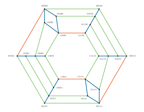
Figure 3: Schlegel diagram of the polytope (43) for $m=2.$ The $24$ vertices are labeled by binary strings. There are four special edges (orange) and $36$ regular ones: $16$ of class $1$ (green) and $20$ of class $2$ (blue). Among the $18$ facets, we see two hexagons and four pentagons.

Proof 5.10 (Sketch of Proof).

Consider a generic vector $w$ in $\mathbb{R}^{6}$ that assigns weights to the six Cox coordinates. The leading monomial $x_{i}s_{j}^{m}t_{k}^{m}$ of $Q$ is determined by the signs of the quantities

(44) $$w(x_{0})-w(x_{1}),\,\,w(s_{0})-w(s_{1}),\,\,w(t_{0})-w(t_{1}).$$

We record this leading monomial in the binary string $ijk.$ Each of these eight choices allows for $m+1$ consistent choices of leading monomials from the tuple $(P_{0},\ldots,P_{m}).$ Indeed, the leading monomial of $P_{\ell}$ coincides with that of $\,\tilde{P}_{\ell}\,\,=\,\,x_{0}s_{0}^{\ell}s_{1}^{m-\ell}t_{0}^{m}\,+\,x_{1}t_{0}^{\ell}t_{1}^{m-\ell}s_{0}^{m}.$ The line segments $\mathcal{N}(\tilde{P}_{\ell})$ lie in translates of a common $2$-dimensional subspace in $\mathbb{R}^{6},$ and their Minkowski sum is a $(2m+2)$-gon. Precisely half of its vertices are compatible with the inequalities (44). These $m+1$ vertices become vertices of (43), and they are all the vertices.

We encode each vertex of (43) by a binary string of length $m+4,$ starting with $ijk.$ The other $m+1$ entries indicate the leading terms of the $P_{\ell}.$ Namely, we write $0$ if the the following expression is positive, and we write $1$ if it is negative:

$$w(x_{0})-w(x_{1})\,+\,(m-\ell)(w(s_{0})-w(s_{1}))\,+\,(m-\ell)(w(t_{0})-w(t_{1}))$$

With this notation, here is the list of all $8(m+1)$ vertices of our polytope:

$$\begin{matrix}000\,1^{{\ell}}0^{m-{\ell}+1}\,,&010\,1^{{\ell}}0^{m-{\ell}+1}\,,&100\,0^{{\ell}+1}1^{m-{\ell}}\,,&110\,0^{{\ell}+1}1^{m-{\ell}}\,,\\ 001\,0^{{\ell}}1^{m-{\ell}+1}\,,&101\,0^{{\ell}}1^{m-{\ell}+1}\,,&011\,1^{{\ell}+1}0^{m-{\ell}}\,,&111\,1^{{\ell}+1}0^{m-{\ell}}\,,\end{matrix}\quad\hbox{for}\,\,{\ell}=0,1,\ldots,m.$$

Any pair of such strings that differs in precisely one entry is an edge of (43). This accounts for all but four of the edges. These special edges are pairs of strings that differ in two positions:

$$\begin{matrix}[000\,0^{m+1}\,,\,001\,0^{m}1],&[000\,1^{m}0\,,\,001\,1^{m+1}],\\ [110\,0^{m+1}\,,\,111\,10^{m}],&[110\,01^{m}\,,\,111\,1^{m+1}].\end{matrix}$$

The other $14m+8$ regular edges come in two classes. In the first class, the initial triple $ijk$ in the binary string is fixed. For each initial triple $ijk$ there are $m$ such edges, for a total of $8m$ edges. The remaining $6m+8$ edges correspond to a sign change in $w(x_{0})-w(x_{1}),$ $w(s_{0})-w(s_{1})$ or $w(t_{0})-w(t_{1}).$ Here, the terminal $m+1$ letters in the binary string is fixed. If that string is $0^{m+1}$ or $1^{m+1}$ then there are four edges which form a square facet of our polytope, namely the square $\,000^{m+2},\,010^{m+2},\,110^{m+2},\,100^{m+2},\,000^{m+2}$ and the square $\,001^{m+2},\,011^{m+2},\,111^{m+2},$ $101^{m+2},\,001^{m+2}.$ For each of the other $2m$ terminal strings, there are only three edges which form a $3$-chain, for instance $0010^{m}1,$ $1010^{m}1,$ $1000^{m}1,$ $1100^{m}1.$ This accounts for all $\,4+8\cdot m+(4+4)+(2m)\cdot 3\,=\,14m+12\,$ edges of our polytope (43).

We now discuss the $6m+6$ facets. First, there are two centrally symmetric $2(m+1)$-gons. They are formed by all strings that start with $00$ or $11$ respectively. There are precisely two other facets adjacent to both $2(m+1)$-gons, namely the two squares facets mentioned above. Adjacent to these two squares and to the two big facets are the four pentagons, which are

$$\begin{matrix}&0000^{m+1},1000^{m+1},1000^{m}1,1010^{m}1,0010^{m}1&&0011^{m+1},0111^{m+1},0111^{m}0,0101^{m}0,0001^{m}0,\\ &1111^{m+1},1011^{m+1},10101^{m},10001^{m},11001^{m}&&1100^{m+1},0100^{m+1},01010^{m},01110^{m},11110^{m}.\end{matrix}$$

Each pentagon contains one of the four special edges. The remaining facets are quadrilaterals. They come in six strips of $m$ facets. See Figure 3 for the case $m=2$.

6 Marginal Likelihood Integrals

We now come to applications of our results to Bayesian statistics. We fix a statistical model $X_{>0}\rightarrow\Delta_{m}$ that is specified by $m+1$ rational functions $p_{i}$ on the toric variety $X.$ These rational functions sum to $1.$ We write $p_{i}(x)=q_{i}(x)/r_{i}(x),$ where the numerator $q_{i}$ and the denominator $r_{i}$ are homogeneous polynomials with positive coefficients that have the same degree in ${\rm Cl}(X).$ We further assume that we are given a rational function $f/g$ that defines a probability distribution $\mu_{f,g}$ on $X_{>0}$ as in (25). This serves as the prior distribution for Bayesian inference.

Remark 6.1.

For the prior distribution on $X_{>0}$ we can choose any two positive polynomials $f$ and $g$ of the same degree in ${\rm Cl}(X)$ such that the relevant integrals converge. This is ensured by the hypothesis on Newton polytopes in Theorem 2.5.

The data comes in the form of $U$ samples from the state space $\{0,1,\ldots,m\}.$ We write $u_{i}$ for the number of samples that are in state $i.$ We assume that the integers $u_{i}$ are positive. They satisfy $u_{0}+u_{1}+\cdots+u_{m}=U.$ Given $u=(u_{0},u_{1},\ldots,u_{m}),$ the likelihood function $L_{u}$ is

(45) $$L_{u}(x)\,\,\coloneqq\,\,\frac{\prod_{i=0}^{m}q_{i}(x)^{u_{i}}}{\prod_{i=0}^{m}r_{i}(x)^{u_{i}}}.$$

This is the probability of observing the data vector $u,$ assuming that the model, the parameters $x,$ and the sample size $U$ are fixed. The Multinomial Theorem implies

$$\qquad\sum_{|u|=U}\frac{U!}{u_{0}!u_{1}!\cdots u_{m}!}\cdot L_{u}(x)\,\,\,=\,\,\,1\qquad\hbox{for all $x\in X_{>0}.$}$$

We are interested in the posterior density on $X_{>0}.$ Up to a constant factor, this is

(46) $$d_{u}\,\,:=\,\,L_{u}\cdot d_{f,g}.$$

The marginal likelihood integral $\,\mathcal{I}_{u}\,$ is the integral of (45) against $\mu_{f,g},$ i.e.,

(47) $$\mathcal{I}_{u}\,\,\,:=\,\,\,\int_{X_{>0}}\!\!L_{u}(x)\,\mu_{f,g}\,\,=\,\,\frac{1}{\mathcal{I}}\int_{X_{>}0}\!\!L_{u}(x)\,\frac{f(x)}{g(x)}\,\Omega_{X}.$$

We shall evaluate $\mathcal{I}_{u}$ using the methods in Section 4, but with $f/g$ replaced by $L_{u}\cdot f/g.$ Also of interest is sampling from the posterior density $d_{u},$ by way of 2.

The Newton polytope of the integrand $\,L_{u}\cdot f/g\,$ admits the decomposition

(48) $$\mathcal{N}(f)\,+\,\mathcal{N}(g)\,+\,\sum_{i=0}^{m}u_{i}\,\mathcal{N}(q_{i})\,+\,\sum_{i=0}^{m}u_{i}\,\mathcal{N}(r_{i}).$$

The normal fan of (48) is independent of the data $u$ since $u_{0},\ldots,u_{m}$ are positive. As before, we let $\mathcal{F}$ be a simplicial refinement of the normal fan of the polytope in (48). We note the following fact, which is important for the applicability of our method.

Observation 6.2.

The simplicial fan $\mathcal{F}$ is independent of the data $u.$ It is computed from the statistical model. This is done in an offline step that is carried out only once per model.

We point out that we may allow some of the $u_{i}$ to be zero. In this case, the true fan is a coarsening of ${\cal F}$. One may still use ${\cal F}$ in our method, at the cost of having more sectors.

The computation of $\mathcal{F}$ is expensive when the dimension $n$ gets larger. Observation 6.2 means that the running time of the algorithms in Sections 3 and 4 is fairly independent of $u.$ For instance, consider the computation of the sector integrals $\mathcal{I}^{\rm tr}_{\sigma}$ using the formula in (19). The data $u$ do not appear in the numerator, but they do enter in the denominator. Namely, the monomial $x^{-\delta_{\sigma}}$ that represents the tropicalized integrand $\,L_{u}^{\rm tr}f^{\rm tr}/g^{\rm tr}\,$ on ${\rm Exp}(\sigma)$ satisfies

$$\delta_{\sigma}\,\,=\,\,\nu_{g}-\nu_{f}\,+\,\sum_{i=0}^{m}u_{i}(\nu_{r_{i}}-\nu_{q_{i}}).$$

In an offline step, done once per model, we precompute the $k\times(m+1)$ matrix of inner products $w_{\ell}\cdot(\nu_{r_{i}}-\nu_{q_{i}}).$ In the online step, with data $u,$ we evaluate (19) rapidly.

One point that does depend on the data $u$ is the accuracy of the approximation in (29). The bounds $M_{1}$ and $M_{2}$ for the function $h$ scale exponentially in $U,$ and hence so does the right hand side of (32). The quality of the estimate $\mathcal{I}_{N}$ can decrease a lot for larger $U$, so that many more samples are needed to obtain an accurate approximation. We observed this phenomenon in our computations. This issue requires further study.

We now present computational experiments with the models we saw in Sections 1 and 5. This material is made available at MathRepo [5]. Our readers can try it out. Our implementation is in Julia. It uses Polymake [6] for polyhedral computations.

Example 6.3 (Coin model).

Consider the coin model from the Introduction. We begin with $m=2.$ Fix $U=5$ and $u=(u_{0},u_{1},u_{2})=(2,1,2).$ The marginal likelihood integral (47) is a rational number. Using symbolic computation as in [10], we find

$$\mathcal{I}_{u}\,\,=\,\,\frac{2267}{1559250}\,\,\approx\,\,0.001454.$$

We reproduce this number using tropical sampling. The Newton polytope (43) of the integrand is shown in Figure 3. Its normal fan has $24$ maximal cones, one for each vertex. But, this fan is not simplicial since eight of the vertices are $4$-valent. We turn (43) into a simple polytope by a small displacement of the facets. The resulting normal fan is simplicial, and it has $32=24+8$ maximal cones. That simplicial fan $\mathcal{F}$ is used for the sector decomposition. The right hand side in (24) has $32$ summands, one for each cone $\sigma\in\mathcal{F}(3).$ The values of the $32$ tropical sector integrals $\mathcal{I}^{\rm tr}_{\sigma}$ are the rational numbers $\,\frac{1}{280},\frac{1}{280},\frac{1}{280},\frac{1}{280},\frac{1}{120},\ldots,\frac{1}{8},\frac{1}{7},\frac{1}{7}.$ Their sum equals $\mathcal{I}^{\rm tr}=\frac{40}{21}=1.9047.$ This gives the discrete probability distribution used in Step 1 of 1. Numerical evaluation of (29) with sample size $N=50000$ yields

$$\mathcal{I}_{N}\,\,=\,\,0.001486.$$

We validated our method with a range of experiments for larger values of $U,m,N.$

Example 6.4 (Pentagon models).

We revisit the linear model and the Wachspress model from Example 5.6. Their common parameter space is the pentagon $P$ with uniform prior. This is lifted to the toric surface $X_{>0}$ with density $d_{f,g}$ given by the homogeneous polynomials $f$ and $g$ in Example 5.3. The coordinates of the two models are obtained from the polynomials in $y$ seen in Example 5.6. We first substitute $y_{1}=\frac{t_{1}}{q}\frac{\partial q}{\partial t_{1}}$ and $y_{2}=\frac{t_{2}}{q}\frac{\partial q}{\partial t_{2}},$ and then we set $t_{1}=x_{1}x_{2}x_{3}^{-1}x_{4}^{-1}$ and $t_{2}=x_{2}^{-1}x_{3}^{-1}x_{4}x_{5}.$ In each case, this yields a rational function $L_{u}f/g$ that is homogeneous of degree zero in $x,$ and satisfies the hypothesis in Theorem 2.5.

The likelihood functions for the linear model and the Wachspress model look similar, but there is a crucial distinction. The latter also involves the adjoint $A.$ This means that statistical inference is different for the two models. For instance, the maximum likelihood (ML) degree of the linear model on $P$ equals five, while the ML degree of the Wachspress model on $P$ equals eight. Recall, e.g. from [8, 14, 15], that the ML degree of an algebraic statistical model is the number of complex critical points of the likelihood function of that model for general data.

Consider the linear model with $(u_{1},u_{2},u_{3},u_{4},u_{5})=(20,16,10,15,23).$ With (41),

(49) $$\mathcal{I}_{u}\,\,\,=\,\,\frac{1}{5^{84}}\cdot\frac{2}{5}\cdot\int_{P}\ell_{1}^{20}\ell_{2}^{16}\ell_{3}^{10}\ell_{4}^{15}\ell_{5}^{23}\,{\rm d}y_{1}{\rm d}y_{2}.$$

For the approximation by tropical sampling, we note that the Newton polygon of $L_{u}f/g$ has seven vertices, so its normal fan $\mathcal{F}$ has $|\mathcal{F}(2)|=7.$ We find that ${\cal I}_{u}\approx 9.652\cdot 10^{-60}.$

We now compare this to the Wachspress model, where the probabilities are products of the linear forms, as shown in (42). We pick the data $(u_{123},u_{234},u_{345},u_{451},u_{512})=(2,3,5,7,11)$ in order to match the exponents of the linear factors in the respective likelihood functions. The marginal likelihood integral for the Wachspress model equals

(50) $$\mathcal{I}_{u}\,\,\,=\,\,2^{13}\cdot\frac{2}{5}\cdot\int_{P}\ell_{1}^{20}\ell_{2}^{16}\ell_{3}^{10}\ell_{4}^{15}\ell_{5}^{23}A^{-84}\,{\rm d}y_{1}{\rm d}y_{2}.$$

where $A=7+2(y_{1}+y_{2})-(y_{1}-y_{2})^{2}$ is the adjoint. Again, the Newton polygon of $L_{u}f/g$ has seven vertices, so its normal fan $\mathcal{F}$ has $|\mathcal{F}(2)|=7.$ We find that ${\cal I}_{u}\approx 1.218\cdot 10^{-66}.$

We next illustrate how our techniques can be applied to Bayesian model selection.

Example 6.5 (Bayes factors).

As before, let $\mu_{f,g}$ denote the prior arising from the toric Hessian. We consider the data $u=(u_{0},u_{1},\ldots,u_{5})=(1,2,4,8,16,32).$ We wish to decide between two models with $n=2$ and $m=5.$ The two competitors are toric models with $p_{i}$ and $Z$ as in Example 5.7, with different coefficient vectors $c=(c_{0},c_{1},\ldots,c_{5}).$ Model $\mathcal{M}_{1}$ is given by $c^{(1)}=(2,3,5,7,11,13)$ while model $\mathcal{M}_{2}$ is given by $c^{(2)}=(32,16,8,4,2,1).$ We denote the respective likelihood functions by $L_{u}^{(1)}$ and $L_{u}^{(2)}$ and the marginal likelihood integrals by

$$\mathcal{I}_{u}^{(i)}\,\,\,=\,\,\int_{X_{>0}}\!\!L_{u}^{(i)}(x)\,\mu_{f,g},\qquad i=1,2.$$

In order to decide which model fits the data better, we compute the ratio $K=\mathcal{I}_{u}^{(1)}/\mathcal{I}_{u}^{(2)}$ of the two marginal likelihood integrals. This ratio is the Bayes factor. Using numerical cubature with tolerance 1e-5, we find that $\mathcal{I}_{u}^{(1)}\approx 5.675\cdot 10^{-38}$ and $\mathcal{I}_{u}^{(2)}\approx 2.694\cdot 10^{-39}.$ Therefore, $K\approx 21.06,$ which reveals that the model $\mathcal{M}_{1}$ is a better fit for $u$ than $\mathcal{M}_{2}.$

Another important Bayesian application is sampling from the posterior distribution. In principle, this can be done with 2, applied to the density $d_{u}$ in (46). However, this fails to work as an off-the-shelf method. At present, the method is of theoretical interest only. The challenge arises from large integer exponents, like $84$ in Equation (50). These exponents lead to a very low acceptance rate in Proposition 4.4. We also observed this in practice: in a typical run of 2 for (49) with $N=100000,$ all samples are rejected.

We conclude that our tropical sampling method rests on solid and elegant mathematical foundations, and it holds considerable promise for Bayesian inference. Yet, more research is needed to make it widely applicable for computational statistics. For larger sample size $U,$ the likelihood function $L_{u}$ has a sharp peak around its maximum, so it will be important to precompute the critical points of $L_{u}.$ The algebraic complexity for this task is the ML degree of the model. This suggests combining tropical sampling with the topological theory of ML degrees. Our experiments also showed that exact symbolic algorithms (cf. [10]) are still surprisingly competitive. For instance, the exact value of the integral $\mathcal{I}_{u}$ in (49) equals

$$\frac{139123\cdot 1256291317\cdot 2602507379\cdot 47336895027767486610187}{2^{4}\cdot 3^{6}\cdot 5^{88}\cdot 7^{2}\cdot\!11\!\cdot 13^{2}\cdot 17^{2}\cdot 19\cdot 23^{2}\cdot 29^{2}\cdot 31^{2}\cdot 37^{2}\cdot 41^{2}\cdot 43\cdot 47\cdot 53\cdot 59\cdot 61\cdot 67\cdot 71\cdot 79\cdot 83}.$$

This rational number is intriguing. We conclude that it would be desirable to combine the methods of Sections 3 and 4 with such exact evaluations. This is left for a future project.

References

• [1] N. Arkani-Hamed, Y. Bai, and T. Lam: Positive geometries and canonical forms, J. High Energy Phys. 11 (2017) 1–124.
• [2] M. Borinsky: Tropical Monte Carlo quadrature for Feynman integrals, Annales de l’Institut Henri Poincaré D, to appear, arXiv:2008.12310, DOI: 10.4171/AIHPD/158.
• [3] D. Cox: Toric residues, Ark. Mat. 34 (1996) 73–96.
• [4] D. Cox, J. Little, and H. Schenck: Toric Varieties, Graduate Studies in Mathematics, vol. 124, American Mathematical Society, 2011.
• [5] C. Fevola and C. Görgen: The mathematical research-data repository MathRepo, Computeralgebra Rundbrief 70 (2022) 16–20.
• [6] E. Gawrilow and M. Joswig: Polymake: a framework for analyzing convex polytopes, Polytopes – Combinatorics and Computation, pages 43–73, Springer, 2000.
• [7] A. Gelman, J.  Carlin, H. Stern, D. Dunson, A. Vehtari, D. Rubin: Bayesian Data Analysis, Third edition, Texts in Statistical Science Series, Chapman & Hall, Boca Raton, FL, 2014.
• [8] S. Hoşten, A. Khetan, and B. Sturmfels: Solving the likelihood equations, Found. Comput. Math. 5 (2005) 389–407.
• [9] M. Kaluba, B. Lorenz, and S. Timme: Polymake.jl: A new interface to polymake, International Congress on Mathematical Software, pages 377–385. Springer, 2020.
• [10] S. Lin, B. Sturmfels, and Z. Xu: Marginal likelihood integrals for mixtures of independence models, J. Mach. Learn. Res. 10 (2009) 1611–1631.
• [11] D. Maclagan and B. Sturmfels: Introduction to Tropical Geometry, Graduate Studies in Mathematics, vol. 161, American Mathematical Soc., 2015.
• [12] L. Nilsson and M. Passare: Mellin transforms of multivariate rational functions, J. Geom. Anal. 23 (2013) 24–46.
• [13] D. Stirzaker: Elementary Probability, $2$nd edition, Cambridge University Press, 2003.
• [14] B. Sturmfels and S. Telen: Likelihood equations and scattering amplitudes, Algebraic Statistics 12 (2021) 167–186.
• [15] S. Sullivant: Algebraic Statistics, Graduate Studies in Mathematics, 194, American Mathematical Society, Providence, RI, 2018.
• [16] S. Telen: Numerical root finding via Cox rings, J. Pure Appl. Algebra 224 (2020), no. 9.
• [17] S. Telen: Introduction to Toric Geometry, arXiv:2203.01690.
• [18] A. J. Walker: New fast method for generating discrete random numbers with arbitrary frequency distributions, Electronics Letters 10 (1974) 127–128.