Infusing nontrivial topology in massive Dirac fermions with scalar potential: Emergence of Scalar Hall Effect

Abstract

We present a simplified way to access and manipulate the topology of massive Dirac fermions by means of scalar potential. We show systematically how a distribution of scalar potential can manipulate the signature of the gap or the mass term as well as the dispersion leading to a band inversion via inverse Klein tunnelling. In one dimension it can lead to the formation of edge localisation. In two dimensions this can give rise to an emergent mechanism, which we refer to as the Scalar Hall Effect. This can facilitate a direct manipulation of topological invariants, e.g. the Chern number, as well as allows to manipulate the edge states locally and thus opens new possibilities for tuning physical observables which originate from the nontrivial topology.

In recent years topology has become a central concept in condensed matter physics Moore (2010), while materials with non-trivial topological properties have become key ingredient in designing next generation transport and memory devices Breunig and Ando (2021); Gilbert (2021). An immense effort has been directed at discovering suitable materials Lin et al. (2015); Ando (2013) and characterization of their topological classes Altland and Zirnbauer (1997); Ryu et al. (2010). This highly active research resulted in the discovery of several new topological phases in the last decade Armitage et al. (2018); Lv et al. (2021). Despite of the phenomenal success these studies still fail to suggest a controllable way to generate the nontrivial topological properties using external stimuli. The first topological insulator, namely the Quantum Hall Insulator, was discovered under strong magnetic field v. Klitzing et al. (1980) which is quite challenging for any practical purpose. In materials with strong spin-orbit-coupling (SOC), such as HgTe Bernevig et al. (2006) or Bi₂Se₃ Zhang et al. (2009), the nontrivial topological features arise from electronic interactions involving orbital and spin degrees of freedom. Such interactions can give rise to different topological phases such as the Quantum Anomalous Hall Insulator Nagaosa et al. (2010) and Quantum Spin Hall Insulator Sinova et al. (2015).

In certain cases it is possible to tune the topological properties with a magnetic field Shamim et al. (2020) or magnetic impurities Cheng et al. (2021); Shamim et al. (2021), however these cases are very material specific which presents a great challenge in their applicability. For most of the cases SOC is considered to be the source of nontrivial topological properties which manifest itself via band inversion Zhu et al. (2012). The band inversion is indeed an impeccable sign of a topological transition, however, on its own it does not directly reflect the specific mechanism which drives it. Besides, it is also possible to have a topological insulator even without SOC or magnetic moment Haldane (1988); Fu (2011) by exploiting the symmetry of electronic degrees of freedom. A proper description of the mechanism behind inducing topological features and the transition dynamics between different topological phases is therefore highly desired in order to access and manipulate the topological phases of solid state systems.

The key to access the non trivial topological properties of these systems lies in their dispersion which resembles that of a relativistic particle. One of the characteristic features of a relativistic dispersion is that each gap is associated with a well defined signature. For any generic Dirac spinor $\psi$ obeying $(i\gamma^{\mu}\partial_{\mu}-m)\psi$=0 (in natural units $c$=$\hbar$=1), where $\gamma^{\mu}$ ($\mu$=0 being the temporal component) are the Dirac matrices obeying the Clifford algebra $\{\gamma^{\mu},\gamma^{\nu}\}$=$2\eta^{\mu\nu}\mathbb{I}$ with $\eta$ being the Minkowski metric, the spectrum has a fundamental gap of $2m$. This is commonly known as the mass-gap since the gap is associated with the rest mass of the particle in relativistic theory. Each energy band is associated with a particular sign of $\langle\gamma^{0}\rangle$ and as a result, each gap can be identified with a specific signature. While the eigenvalue spectra remain the same irrespective of the sign of $m$, the eigenstates are sensitive to it and manifest different topological features. A pronounced example is the appearance of Jackiw-Rabi modes at the boundary of two different domains characterised by opposite mass terms Jackiw and Rebbi (1976) where the topological phase boundary is manifested as spatial localisation which is the essence of edge states in topological insulators.

To understand the relation between the mass term and topological characteristics of a system, let us consider a generic $2\times 2$ Dirac Hamiltonian $\bm{\sigma}\cdot\bm{n}(\bm{R})$ defined on Bloch sphere, where $\bm{\sigma}$ is the vector of Pauli matrices and $\bm{n}(\bm{R})$ is the unit vector parameterised by $\bm{R}$. In this case the vector Berry curvature is simply given by $\bm{n}$ Xiao et al. (2010). In two dimensions, two of the Pauli matrices are coupled with momentum corresponding to the direction of motion while the third is coupled to the mass term. The Chern number in this case follows the same signature of the out of plane component of $\bm{n}$, which is nothing but the mass term. Similar correlation has been observed in two-dimensional paramagnetic systems and three dimensional complex heterostructures as well Ghosh and Manchon (2019). In a condensed matter system the mass term is associated with a order parameter and therefore can be exploited to identify different phases Ghosh and Manchon (2016). A simple way to manipulate the magnitude and signature of the mass-gap thus has an enormous potential in fabricating topologically non trivial systems and exploring their applications.

In this work, taking a generic two band system as a prototype, we present a systematic analysis of the topological properties in a multi-band system and demonstrate a simplified way to generate and manipulate non-trivial topological features with the help of scalar potential. In practice, such scalar potential can be introduced by the means of nano-patterning Barad et al. (2021) or surface super lattice Esaki and Tsu (1970). By using the two-band Dirac Hamiltonian, we demonstrate how one can manipulate the mixture of different quantum states which in turn controls the topological features. The formalism is applicable to a large class of condensed matter systems, which facilitates a wide range of applications of this generic protocol.

I Dirac equation in one dimension

In one dimension, it is sufficient to consider the $2\times 2$ representation of Dirac matrices, which we choose here as the Pauli matrices ($\bm{\sigma}$). We define our system with the one dimensional Dirac Hamiltonian

$$H_{1}^{D}=-i\sigma_{1}\partial_{x}+\sigma_{3}m+\sigma_{0}V(x).$$ (1)

where $V(x)$ is a scalar potential $\sigma_{0}$ is the identity matrix of rank 2. In absence of the potential term, the energy spectrum consists of two hyperbolic branches ($E=\pm\sqrt{p^{2}+m^{2}}$, $p$ being the momentum) separated by a gap of $2m$ with positive and negative energy eigen values characterised by positive and negative values of $\langle\sigma_{3}\rangle$. For such a system, it is possible to achieve complete transmission if the barrier height is greater than twice the mass term ($V_{0}>2m$) (Appendix A). This is known as the Klein paradox Klein (1929) which has attracted a lot of interest in both high energy physics as well as in condensed matter physics Katsnelson et al. (2006). The simplest way to understand the underlying mechanism is via the intermixture of states with positive and negative energy. If the scalar potential is strong enough ($V_{0}>2m$), then it can elevate the negative energy states inside the potential barrier to an energy level occupied by the positive energy states outside the barrier which creates a continuous channel using plane-wave modes. For smaller barrier width, interference due to finite size effect is more prominent which is manifested as a periodic oscillation in transmission probability (Appendix A).

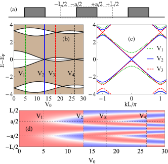
Figure 1: Variation of mass-gap with $V_{0}$. (a) Schematic of the one-dimensional periodic lattice. The dashed box shows the unit cell and the gray boxes show the scalar potential $V_{0}$. (b) Variation of band width (filled region) with the applied potential. White regions correspond to the band gap. (c) Band structure for selected values of $V_{0}$ marked by vertical coloured lines in (b). (d) Distribution of the order parameter $\Delta(x)$ over the unit cell with respect to $V_{0}$ where red and blue colour represent the positive and negative magnitude respectively.

The physics becomes more intriguing if such potential region is employed periodically which can create states with alternating sign of the mass term in successive regions in space. As a result, although the scalar potential itself cannot alter the mass gap, the interference between states with different mass terms can alter the characteristic band gap. To demonstrate this effect we consider one-dimensional Dirac-Kronig-Penney model which has been used to analyse relativistic quarks McKellar and Stephenson (1987) and fermions Ghosh and Saha (2014). Here we consider a one dimensional lattice with length $L$ (set to be 1) and with a rectangular potential of height $V_{0}$ and width $a$ such that $a/L=0.4$ and calculate the band structure (Fig. 1). We define the spatial order parameter

$$\Delta(x)=\left[(\langle+,x|\sigma_{3}|+,x\rangle-\langle-,x|\sigma_{3}|-,x\rangle)/2\right]_{k=0}$$ (2)

where $|+,x\rangle$ and $|-,x\rangle$ denote the wave function at $x$ of the lowest positive energy and highest negative energy states. For $V_{0}$=0 these two states reside at energy $E$=$\pm m$. For $V_{0}>$0, both of these states are shifted by a positive value. To keep these two states symmetric around the zero level we subtract a fixed energy $E_{F}$ for each value of $V_{0}$. This energy is analogous to the Fermi level in a system with finite number of particles.

From Fig. 1 one can see that by increasing the barrier height it is possible to manipulate the mass gap. The mass gap decreases due to the fact that the potential $V_{0}$ now pulls up negative energy states within the window $-m<E<m$ which can now tunnel through the region without potential where the evanescent modes have opposite signature of the mass term. In a sense, this is the Inverse Klein Tunnelling where the tunnelling happens through the potential free region. This mechanism promotes more mixing of quantum states which creates a spatial modulation of the order parameter $\Delta$. Note that at some critical values the gap vanishes completely ($V_{2}$, $V_{4}$ in Fig. 1), and the distribution of the order parameter also flips sign. This critical potential is minimum when the barrier width is half of the unit cell which maximises the mixture of quantum states (Fig. 2). The flipping of the order parameter establishes that each of these crossings is actually associated with a band inversion. The impact of the band inversion will become more clear when we explore the topological properties of a two-dimensional model in the next section.

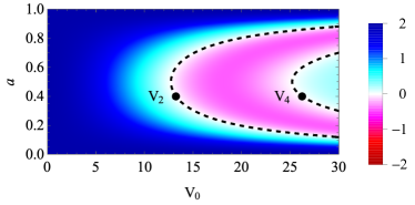
Figure 2: Variation of mass gap with the barrier width ($a$) and barrier height ($V_{0}$). The colour shows the value of the mass gap multiplied by the sign of the order parameter at $x$=0 and the black dashed lines show the transition boundary for the mass term. $V_{2}$ and $V_{4}$ shows the location of transition point in Fig. 1.

II Lattice model: From 1D to 2D

Transition from continuum to a lattice model for a relativistic Hamiltonian is not a straight forward task. Since we are not looking into chiral fermions here, we are free from the obstacles imposed by the Nielson-Ninomiya theorem Nielsen and Ninomiya (1981). For modelling the massive/gapped Fermions, one can follow Wilson’s prescription and introduce a coupling between the spinors to construct a relativistic lattice Hamiltonian. However this approach is not free from doublers (Wilson, 1974). To get rid of the doublers, here we adopt the Hamiltonian prescribed by Creutz and Horvath Creutz and Horváth (1994) which is also known as Creutz lattice. For a two component spinor field $\psi=[a,b]^{T}$ the Creutz Hamiltonian can be expressed as

$$H_{C} = iA\sum_{j}a_{j+1}^{\dagger}a_{j}-a_{j}^{\dagger}a_{j+1}-b_{j+1}^{\dagger}b_{j}+b_{j}^{\dagger}b_{j+1}$$ (3)

$$- B\sum_{j}a_{j+1}^{\dagger}b_{j}+b_{j+1}^{\dagger}a_{j}+M\sum_{j}a_{j}^{\dagger}b_{j}+b_{j}^{\dagger}a_{j}.$$

For convenience we perform a unitary transformation $H_{1}=U^{\dagger}H_{C}U$ [where $U$=$(\sigma_{1}+\sigma_{3})/\sqrt{2}$]. The transformed Hamiltonian in reciprocal space is given by $H_{1}(k)$=$[M-2B\cos(k)]\sigma_{3}+2A\sin(k)\sigma_{1}$. Although the physical outcome doesn’t change under such unitary transformation, the modified form makes it easier to correlate our prediction with known physical system which would be more clear when we discuss the scenario in two dimensions.

II.1 Tuning topological phase in 1D: Emergence of edge localisation

We start from the lattice Hamiltonian in one dimension given by

$$H_{1}(k)=(M-2B\cos(k))\sigma_{3}+2A\sin(k)\sigma_{1}$$ (4)

One can readily see that for $k\to 0$, the low energy spectrum correspond to the continuum Dirac Hamiltonian (Eq. 1) with a mass gap of $M-2B$. Here we choose $M=A=5.0$ and $B=2.0$, and a unit cell with $L=40$ sites. A scalar potential of strength $V_{0}$ is spanned over a region of $a=16$ sites, i.e. $40\%$ of it is covered with the scalar potential. In absence of any scalar potential the system has a mass $M-2B$=1 which is same as the continuum limit. The Fermi level corresponds to half filling and is kept at 0. We define a site-resolved order parameter

$$\Delta_{i}=\left[(\langle+,i|\sigma_{3}|+,i\rangle-\langle-,i|\sigma_{3}|-,i\rangle)/2\right]_{k=0},$$ (5)

where $|+,i\rangle$ and $|-,i\rangle$ is the wave function at site $i$ of the lowest positive energy and highest negative energy states.

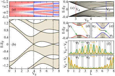
Figure 3: Tuning the phases of a 1D chain. (a) Variation of site resolved order parameter $\Delta_{i}$ with $V_{0}$ in a one-dimensional model. (b) Variation of band gap with $V_{0}$. (c) Variation of energy eigenvalues of a finite chain (dotted lines). Shaded region shows the energy range spanned by periodic chain. Vertical red and blue dashed line show two specific values of $V_{0}$ ($V_{d}$=3 and $V_{e}$=5 respectively). (d) and (e) show the band structure close to $k$=0 for $V_{0}$=$V_{d}$ and $V_{0}$=$V_{e}$ marked with red and blue dashed lines in (c). The horizontal black lines show the energy level of finite system. (e) and (f) show the probability density of highest occupied ($\psi_{1}$) and lowest unoccupied ($\psi_{2}$) states marked with orange and green arrows in (d) and (e) respectively. $L$ denotes length in units of unit cell and the gray regions denote the potentials.

From Fig. 3a one can readily see that the mass term behaves in a similar manner compared to continuum model with respect to $V_{0}$. The variation of the band gap in the lattice model (Fig. 3b) is also qualitatively the same as the prediction of the continuum model. This establishes the validity of the lattice model for our study. From the band structure one can see that the distribution of the mass term switches sign as it passes through a band crossing (denoted by vertical black dashed lines in Fig. 3a,b). To understand if these jumps are associated with any change in topological phase, we consider a super cell with 8 unit cells (total 320 sites) and with open boundary condition. We consider two different strengths of the scalar potential ($V_{d}$ and $V_{e}$ in Fig. 3c) on either side of the crossing point. One can readily see that after the critical potential, the finite chain has eigenvalues close to zero energy (Fig. 3b inset). The eigenstates corresponding to these zero energy modes are strongly localised near the edges (Fig. 3g) whereas before transition the highest occupied and lowest unoccupied states are localised in the bulk (Fig. 3f). One can see that the system is essentially behaving like a SSH model Su et al. (1979) where the variation of hopping parameter can be achieved with the scalar potential. This clearly indicates that one can tune the mass of the system with a scalar potential which in turn can influence the topology of the system. This connection will be more clear in next section where we discuss about the two dimensional systems.

II.2 Tuning topological phase 2D: Emergence of helical edge mode

The extension of Hamiltoninan $H_{1}$ (Eq. 4) to two dimensions is quite straightforward and is given by

$$H_{2}(k_{x},k_{y}) = [M-2B(\cos(k_{x})+\cos(k_{y}))]\sigma_{3}$$ (6)

$$+2A[\sin(k_{x})\sigma_{1}+\sin(k_{y})\sigma_{2}].$$

One can easily recognise that this is the $2\times 2$ block of the Hamiltonian used to define the quntum spin Hall effect in HgTe-CdTe quantum wells, commonly known as the Bernevig-Hughes-Zhang (BHZ) model Bernevig et al. (2006). The Creutz lattice (Eq.3) and the BHZ model (Eq.6) are the simplest models of a Chern insulators. In the following sections we use the BHZ model which exhibits a Chern number $\mathcal{C}=sgn(M)$ for $|M|<|4B|$ and $\mathcal{C}=0$ for $|M|>|4B|$. This lends us a perfect playground for further predictions. We start with $M=9$, $B=2$ and $A=5$ which gives a trivial Chern insulator state ($\mathcal{C}=0$). The mass-gap at $k_{x},k_{y}=0$ is given by $M-4B$ which for our choice of parameters is 1. Here we consider a $3\times 3$ supercell with one scalar potential (resulting in 11.1% coverage) and calculate the variation of band structure, mass term and the Chern number (Fig. 4) with the variation of $V_{0}$.

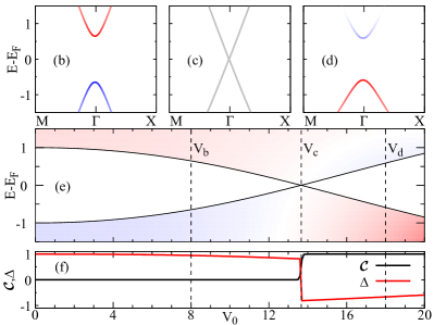
Figure 4: Variation of topological nature with $V_{0}$. (a) Schematic of the super cell lattice with $3\times 3$ motif. Dark brown blocks correspond to areas with an additional scalar potential. (b-d) show the band structure for $V_{0}=V_{b},V_{c},V_{d}$, respectively (shown by vertical dashed line in (e)) with red (blue) colour showing positive/negative values of $\langle\sigma_{3}\rangle$. (e) shows the variation of the band gap with $V_{0}$ where red (blue) colour corresponds +ve(-ve) value of $m(E)$. (f) shows the variation of the Chern number (black) and the total order parameter $\Delta$ (red) with $V_{0}$.

The Chern number can be calculated from

$$\mathcal{C} = \frac{1}{2\pi}\sum_{n}^{n_{F}}\int_{BZ}dk_{x}dk_{y}[f(E_{n})-f(E_{m})]\times$$ (7)

$$\sum_{m\neq n}2~{}{\rm Im}\left[\frac{\langle m|\partial H/\partial k_{y}|n\rangle\langle n|\partial H/\partial k_{x}|m\rangle}{(E_{n}-E_{m})^{2}+\eta^{2}}\right]$$

where $n_{F}$ is the number of states below the Fermi level. $f(E_{n})$ is the Fermi-Dirac distribution for the $n$th energy eigenvalue and $|n\rangle$ is the $n$th eigenstate. $\eta$ is the constant broadening which we choose to be 0.005. The mass term at any particular energy is given by

$$m(E)=\int_{BZ}dk_{x}dk_{y}\sum_{n}^{2N}\langle n|\sigma_{3}\otimes\mathbb{I}_{N}|n\rangle\delta(E_{n}-E),$$ (8)

where $N$ is the number of sites (which for our case is 9) and $\mathbb{I}_{N}$ is the identity matrix of rank $N$. $\delta(x)$ is the Dirac delta function which is approximated as a Lorentzian with broadening $\eta$. For simplicity, instead of space resolved order parameter, we use the integrated order parameter defined as

$$\Delta=[(\langle+|\sigma_{3}\otimes\mathbb{I}_{N}|+\rangle-\langle-|\sigma_{3}\otimes\mathbb{I}_{N}|-\rangle)/2]_{k=0}.$$ (9)

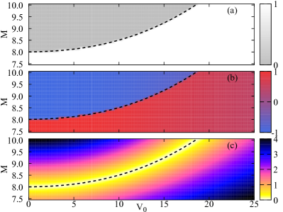
Figure 5: Variation of (a) Chern number ($\mathcal{C}$), (b) order parameter ($\Delta$) and (c) mass gap with the parameter $M$ and strength of scalar potential ($V_{0}$). Black dashed line shows the transition boundary.

With these definitions one can clearly see the connection between the band inversion and the mass (Fig. 4) in two dimensions as well. From Fig. 4, one can see that with the increase of the scalar potential, there is a band gap closing and reopening, similar to what we observe in the one-dimensional case (Fig. 1,3). At the critical point, where the bands touch each other, the order parameter as well as the Chern number undergo a jump indicating a change of the topological phase. This is consistent with our earlier picture of band inversion through the mixing of different mass regimes. The non-zero Chern number indicates the generation of a Hall current due to the scalar potential. Since the effect is triggered by a scalar term rather than a vector field, we call it Scalar Hall Effect to distinguish it from the existing Hall effects. This is an emergent effect caused by the mixture of quantum states mediated by the scalar potential. In a topologically trivial regime each occupied band is comprised of states with the same sign of the mass term. As we increase the potential, the interchange of states with opposite mass term takes place. Increase of the scalar potential enhances the mixing of states with opposite mass term and thus transports the system from a topologically trivial to non trivial phase, characterised by a non-zero Chern number. The critical potential ($V_{C}$ in Fig. 4) at which the transition takes place shows a parabolic dependence with respect to the parameter $M$ that controls the mass of the system (Fig. 5) and a logarithmic behaviour with respect to the potential concentration (Fig. 6).

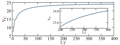
Figure 6: Variation of critical potential $V_{C}$ with the density of scalar potential $f$.

In contrast to random disorder induced Chern insulator Kuno (2019), this mechanism is intrinsic in nature. This is reflected in the fact that the emergent non trivial phase possesses same magnitude of gap compared to the potential free case whereas the disorder induced non trivial phase is known to have order of magnitude smaller gap Kuno (2019). The underlying mechanism is also distinct from the previously reported mechanism for voltage modulated Chern number Jiang et al. (2010) where one can arbitrarily enhance the Chern number by increasing the voltage. Our mechanism, on the other hand, facilitates a transition from $\mathcal{C}$=0 to $\mathcal{C}$=1, which is the highest Chern number possible for this model. If one starts from a topologically non-trivial configuration, the additional scalar potential enhances the topological protection and reduce mixing of quantum states and thus prevents any further topological transition (Fig. 5).

III Formation and manipulation of edge states:

A non-vanishing bulk topological invariant shares a direct correspondence with the existence of edge states Hatsugai (1993); Qi et al. (2006). To demonstrate that, we consider a ribbon configuration, i.e. we assume a periodic boundary condition along $x$-direction, and open boundary condition along $y$-direction by repeating the block shown in Fig. 4a. Here we choose 3 sites along $x$ and 90 sites along $y$ (total 270 sites, Fig. 7) and introduce scalar potential $V_{0}$ in one in every nine ($3\times 3$) sites ($11.1\%$ coverage).

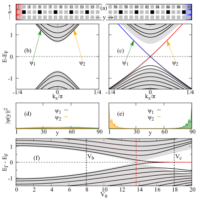
Figure 7: Variation of bulk and edge properties with $V_{0}$. (a) The schematic of the ribbon with scalar potentials denoted in black. (b) and (c) show the band structure for $V_{0}$=$V_{b}$ and $V_{0}$=$V_{c}$ ($V_{b}$ and $V_{d}$ in Fig. 4e). Red, blue and black colors mark the contribution from the edge at $y$=1, edge at $y$=90 and the bulk region. Gray shaded region marks the region spanned by the bulk bands. (d),(e) show the probability density of the state $\Psi_{1,2}$, marked with green and orange arrow in (a),(b). (c) shows the variation of eigenvalues at the $\Gamma$-point where the black and red colour correspond the contribution from the bulk and edges. The gray region shows the area spanned by the bulk bands and the vertical red dashed line shows the point of band inversion ($V_{0}$=$V_{c}$ in Fig. 4c,e,f).

In such a ribbon the edge states emerge when $V_{0}$ crosses the critical value at which the bulk bands cross each other (Fig. 7). This is similar to the emergence of edge localisation in 1D system (Fig. 4). Each edge hosts a single edge state such that opposite edges host states with an opposite group velocity, which is expected in case of a Chern insulator with a Chern number of 1.

One can further manipulate the behaviour of the edge states locally by controlling the distribution of the scalar potential. As we explained before, the scalar potential enhances the mixing between the states with an opposite mass term which causes the topological transition. In an extended system, one can use the the scalar potential selectively in different regions of space to infuse the topological nature selectively. To demonstrate this we consider the aforementioned ribbon (Fig. 7). Then we start removing the scalar potential from one end and calculate the band structure (Fig. 8). The Fermi level ($E_{F}$) is defined as the middle of 270$th$ and 271$th$ eigenvalue at the $\Gamma$-point.

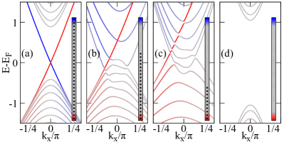
Figure 8: Variation of the band structure with the distribution of the scalar potential along the ribbon. (a) The band structure when the full width of the ribbon is covered with the potential. (b,c) show the band structure with 2/3- and 1/3-coverage, and (d) shows the band structure with no potential. Inset of each figure shows the spatial distribution where the black dots represent the scalar potential. Red and blue colours denote the $y$=1 and $y$=90 edges (Fig. 7a).

With this simple procedure one can easily manipulate the edges states selectively. By removing the scalar potential at one edge, we reduce the mixing of the states locally and as a result, the states which were sharply localised at the edges before now start moving more into the central region. This is manifested by the fact that the sharp red line in Fig. 8 remains intact as long as there are scalar potentials at the corresponding edges whereas the blue lines fade out and mix strongly with the gray bands.

IV Random orientation of potential

The obvious question that arises at this point is whether this is an artefact of a perfect periodic system or not. To answer that we consider a $12\times 12$ super cell with 16 scalar potential ($11.1\%$ coverage) and calculate the variation of mass gap (Fig. 9). Since calculating Chern number for such large system is computationally quite demanding, we calculate it for two different topological phases. One can readily see that the mass gap and the topological features changes in a similar way as the small and uniform supercell (Fig. 4) which establishes that it is an intrinsic property and doesn’t depend on the distribution of scalar potential. Similar behaviour can be observed with a ribbon with open boundary condition along $y$ direction (Fig. 10). We choose a super cell of $15\times 60$ sites and scatter 100 scalar potential with $V_{0}$=20. Here we also observe a pair of helical edge states similar to the case of uniform distribution (Fig. 7). Note that there are small asymmetry in the bulk states which comes from the assymetric distribution of the scalar potential. However it doesn’t effect the presence of the edge states. These results confirm that the topological transition can be achieved with scalar potential for any arbitrary distribution.

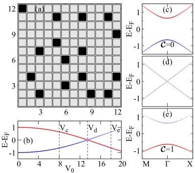
Figure 9: Variation of mass gap and Chern number for super cell. (a) Distribution of potential (black blocks) over the supercell. (b) Variation of band gap where the red and blue colour denote positive and negative values of $\langle\sigma_{z}\rangle$. (c),(d) and (e) show band structure and Chern number for three different values of $V_{0}$ denoted by vertical dashed line in (b).

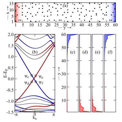
Figure 10: Edge state formation for extended ribbon. (a) Distribution of potential over the ribbon. (b) Band structure of the ribbon where red and blue colour show the contribution from $y$=1 and $y$=60 edges. (c),(d),(e) and (f) show the average probability density along x axis of four different states marked in (b).

V Conclusions

In this paper we present a new paradigm to infuse non-trivial topological characteristics into a trivial insulator by means of a scalar potential. The scalar potential is utilised to enhance the mixing between different quantum states which in turn drives the system into a topologically non-trivial regime accompanied by a reversal in mass term. This switching is present in both one and two dimensions. In one dimension, it produces strong edge localisation whereas in two dimensions it shows appearance of the helical edge states with specific group velocity. It two dimensions, it gives rise to an emergent Hall effect which can be verified by calculating the Chern number. In addition our method also allows to control the topological properties by local means, which is not possible with a topological insulator. We demonstrate that the edge states can be controlled by selective placement of the scalar potential. One can observe the same qualitative behaviour with a periodic as well as non-periodic distribution of scalar potential as long as it doesn’t form clusters. These predictions can be realised in real materials available experimentally. A suitable candidate for such study would be a CdTe-HgTe-CdTe quantum well where the topological phases can be controlled by changing the width of the well. The scalar potential can be designed with suitable fabrication techniques Caro et al. (1986); Wang et al. (2020) or can be introduced via nonmagnetic dopant. For Hg_0.32Cd_0.68Te-HgTe quantum well, the mass gap ($2m$) is $\sim$50 meV for a thickness of 50 $\rm\AA$ Bernevig et al. (2006) which indicates the scalar potential induced topological transition can be observed for $V_{0}\lesssim 0.5$ eV. Our results thus open several new possibilities to control the topological properties and designing highly controllable devices for topological electronics.

VI Acknowledgments

SG would like to acknowledge helpful discussions with Emil Prodan. The work is supported by the Deutsche Forschungsgemeinschaft (DFG, German Research Foundation) $-$ TRR 173/2 $-$ 268565370 (project A11), TRR 288 $-$ 422213477 (project B06).

Appendix A Transmission of massive Dirac particle in one dimension through a rectangular barrier

Here we briefly show the transmission of a massive Dirac particle through a scalar potential which can provide a better understanding of the modulation of the mass term. We start with a massive Dirac equation in one dimension given by

$$H_{1}^{D}=-i\sigma_{1}\partial_{x}+\sigma_{3}m+\sigma_{0}V(x).$$ (10)

where $m$ is the mass term which we choose to be 1. $\sigma_{1,3}$ are the Pauli matrices and $\sigma_{0}$ is the identity matrix of rank 2. The simplest way to study the impact of a scalar potential is to introduce a rectangular barrier of width $w$, such that $V(x)=V_{0}$ for $-w/2\leq x\leq w/2$ and $V(x)=0$ otherwise. The transmission probability for such a rectangular barrier is given by $T=16|\lambda/((1+\lambda)^{2}e^{-i\kappa_{2}w}-(1-\lambda)^{2}e^{i\kappa_{2}w}|^{2}$ where $\kappa_{1}=\sqrt{E^{2}-m^{2}}$ and $\kappa_{2}=\sqrt{(E-V_{0})^{2}-m^{2}}$ and $\lambda=\frac{\kappa_{2}}{\kappa_{1}}\frac{E+m}{E-V_{0}+m}$. For such a system, it is possible to achieve complete transmission probability if the the barrier height is greater than twice the mass term ($V_{0}>2m$). which is manifested as multiple transmission channels for $E<V_{0}$ in Fig. 11.

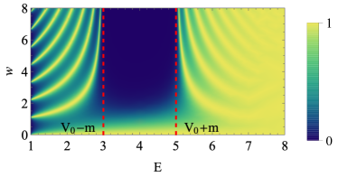
Figure 11: Variation of transmission probability for different energy and barrier width in case of a rectangular barrier introduced in a one-dimensional Dirac Hamiltonian. Here we choose $V_{0}$=4 and $m$=1.

For $w\to\infty$, the Klein window ($m\leq E\leq V_{0}-m$) can manifest complete transmission. At this limit the the region inside and outside the scalar potential are dominated by a particular sign of the mass term. For small $w$, there is more mixture between the states with different mass term which manifests itself as a modulation of the transmission probability with respect to the energy on the both side of the forbidden zone ($V_{0}-m\leq E\leq V_{0}+m$). In a periodic lattice with fixed width of the potential region, this interference results in a modulation of mass-gap with respect to the barrier height $V_{0}$.

References

- Moore (2010) J. E. Moore, Nature 464, 194 (2010).
- Breunig and Ando (2021) O. Breunig and Y. Ando, Nat. Rev. Phys. (2021), 10.1038/s42254-021-00402-6.
- Gilbert (2021) M. J. Gilbert, Commun. Phys. 4 (2021), 10.1038/s42005-021-00569-5.
- Lin et al. (2015) S.-Y. Lin, M. Chen, X.-B. Yang, Y.-J. Zhao, S.-C. Wu, C. Felser, and B. Yan, Phys. Rev. B 91, 094107 (2015).
- Ando (2013) Y. Ando, J. Phys. Soc. Japan 82, 102001 (2013).
- Altland and Zirnbauer (1997) A. Altland and M. R. Zirnbauer, Phys. Rev. B 55, 1142 (1997).
- Ryu et al. (2010) S. Ryu, A. P. Schnyder, A. Furusaki, and A. W. W. Ludwig, New. J. Phys. 12, 065010 (2010).
- Armitage et al. (2018) N. P. Armitage, E. J. Mele, and A. Vishwanath, Rev. Mod. Phys. 90, 015001 (2018), arXiv:1705.01111 .
- Lv et al. (2021) B. Lv, T. Qian, and H. Ding, Rev. Mod. Phys. 93, 025002 (2021).
- v. Klitzing et al. (1980) K. v. Klitzing, G. Dorda, and M. Pepper, Phys. Rev. Lett 45, 494 (1980).
- Bernevig et al. (2006) B. A. Bernevig, T. L. Hughes, and S.-C. Zhang, Science 314, 1757 (2006).
- Zhang et al. (2009) H. Zhang, C.-X. Liu, X.-L. Qi, X. Dai, Z. Fang, and S.-C. Zhang, Nat. Phys. 5, 438 (2009).
- Nagaosa et al. (2010) N. Nagaosa, J. Sinova, S. Onoda, A. H. MacDonald, and N. P. Ong, Rev. Mod. Phys. 82, 1539 (2010).
- Sinova et al. (2015) J. Sinova, S. O. Valenzuela, J. Wunderlich, C. Back, and T. Jungwirth, Rev. Mod. Phys. 87, 1213 (2015).
- Shamim et al. (2020) S. Shamim, W. Beugeling, J. Böttcher, P. Shekhar, A. Budewitz, P. Leubner, L. Lunczer, E. M. Hankiewicz, H. Buhmann, and L. W. Molenkamp, Sci. Adv. 6 (2020), 10.1126/sciadv.aba4625.
- Cheng et al. (2021) E. Cheng, W. Xia, X. Shi, H. Fang, C. Wang, C. Xi, S. Xu, D. C. Peets, L. Wang, H. Su, L. Pi, W. Ren, X. Wang, N. Yu, Y. Chen, W. Zhao, Z. Liu, Y. Guo, and S. Li, Nat. Commun. 12 (2021), 10.1038/s41467-021-26482-7.
- Shamim et al. (2021) S. Shamim, W. Beugeling, P. Shekhar, K. Bendias, L. Lunczer, J. Kleinlein, H. Buhmann, and L. W. Molenkamp, Nat. Commun. 12 (2021), 10.1038/s41467-021-23262-1.
- Zhu et al. (2012) Z. Zhu, Y. Cheng, and U. Schwingenschlögl, Phys. Rev. B 85, 235401 (2012).
- Haldane (1988) F. D. M. Haldane, Phys. Rev. Lett. 61, 2015 (1988).
- Fu (2011) L. Fu, Phys. Rev. Lett. 106, 106802 (2011), arXiv:1010.1802 .
- Jackiw and Rebbi (1976) R. Jackiw and C. Rebbi, Phys. Rev. D 13, 3398 (1976).
- Xiao et al. (2010) D. Xiao, M.-C. Chang, and Q. Niu, Rev. Mod. Phys. 82, 1959 (2010), arXiv:0907.2021 .
- Ghosh and Manchon (2019) S. Ghosh and A. Manchon, Phys. Rev. B 100, 014412 (2019), arXiv:1901.08314 .
- Ghosh and Manchon (2016) S. Ghosh and A. Manchon, SPIN 06, 1640004 (2016), arXiv:1605.02207 .
- Barad et al. (2021) H.-N. Barad, H. Kwon, M. Alarcón-Correa, and P. Fischer, ACS Nano 15, 5861 (2021).
- Esaki and Tsu (1970) L. Esaki and R. Tsu, IBM J. Res. Dev. 14, 61 (1970).
- Klein (1929) O. Klein, Zeitschrift für Phys. 53, 157 (1929).
- Katsnelson et al. (2006) M. I. Katsnelson, K. S. Novoselov, and A. K. Geim, Nat. Phys. 2, 620 (2006), arXiv:0604323 [cond-mat] .
- McKellar and Stephenson (1987) B. H. J. McKellar and G. J. Stephenson, Phys. Rev. C 35, 2262 (1987).
- Ghosh and Saha (2014) S. Ghosh and A. Saha, Eur. Phys. J. B 87, 167 (2014).
- Note (1) In continuum limit, a filled Dirac sea contains infinite number of particles and the notion of Fermi level is not well defined.
- Nielsen and Ninomiya (1981) H. Nielsen and M. Ninomiya, Phys. Lett. B 105, 219 (1981).
- Wilson (1974) K. G. Wilson, Phys. Rev. D 10, 2445 (1974).
- Creutz and Horváth (1994) M. Creutz and I. Horváth, Phys. Rev. D 50, 2297 (1994).
- Su et al. (1979) W. P. Su, J. R. Schrieffer, and A. J. Heeger, Phys. Rev. Lett. 42, 1698 (1979).
- Kuno (2019) Y. Kuno, Phys. Rev. B 100, 054108 (2019), arXiv:1905.11849 .
- Jiang et al. (2010) Z.-F. Jiang, R.-L. Chu, and S.-Q. Shen, Phys. Rev. B 81, 115322 (2010).
- Hatsugai (1993) Y. Hatsugai, Phys. Rev. Lett. 71, 3697 (1993).
- Qi et al. (2006) X.-L. Qi, Y.-S. Wu, and S.-C. Zhang, Phys. Rev. B 74, 045125 (2006).
- Caro et al. (1986) J. Caro, E. van der Drift, K. Hagemans, and S. Radelaar, Microelectron. Eng. 5, 273 (1986).
- Wang et al. (2020) D. Q. Wang, D. Reuter, A. D. Wieck, A. R. Hamilton, and O. Klochan, Appl. Phys. Lett. 117, 032102 (2020).