LyMAS reloaded: improving the predictions of the large-scale Lyman-$\alpha$ forest statistics from dark matter density and velocity fields

Abstract

We present LyMAS2, an improved version of the “Lyman-$\alpha$ Mass Association Scheme” aiming at predicting the large-scale 3d clustering statistics of the Lyman-$\alpha$ forest (Ly-$\alpha$) from moderate resolution simulations of the dark matter (DM) distribution, with prior calibrations from high resolution hydrodynamical simulations of smaller volumes. In this study, calibrations are derived from the Horizon-AGN suite simulations, (100 Mpc/h)³ comoving volume, using Wiener filtering, combining information from dark matter density and velocity fields (i.e. velocity dispersion, vorticity, line of sight 1d-divergence and 3d-divergence). All new predictions have been done at $z=2.5$ in redshift-space, while considering the spectral resolution of the SDSS-III BOSS Survey and different dark matter smoothing (0.3, 0.5 and 1.0 Mpc/h comoving). We have tried different combinations of dark matter fields and found that LyMAS2, applied to the Horizon-noAGN dark matter fields, significantly improves the predictions of the Ly-$\alpha$ 3d clustering statistics, especially when the DM overdensity is associated with the velocity dispersion or the vorticity fields. Compared to the hydrodynamical simulation trends, the 2-point correlation functions of pseudo-spectra generated with LyMAS2 can be recovered with relative differences of $\sim$5% even for high angles, the flux 1d power spectrum (along the light of sight) with $\sim$2% and the flux 1d probability distribution function exactly. Finally, we have produced several large mock BOSS spectra (1.0 and 1.5 Gpc/h) expected to lead to much more reliable and accurate theoretical predictions.

1 Introduction

Distant quasars emit light that crosses a large part of the Universe before being observed with instruments on Earth. In particular, the spectrum of each quasar presents fluctuating absorption that corresponds to the Lyman-$\alpha$ forest (Ly-$\alpha$, Lynds (1971); Sargent et al. (1980)). The study of the Lyman-$\alpha$ forest has become a major focus of modern cosmology, as it is supposed to trace the neutral hydrogen density that fills most of the Universe in a way that approximately corresponds to the underlying dark matter density (Croft et al., 1999; Peeples et al., 2010). Since a single background source only provides one dimensional information along the corresponding line-of-sight (or “skewer”), characterizing the 3d density of the high redshift Universe with the Ly-$\alpha$ forest requires large samples of quasar spectra. Successful surveys such as the (extended) Baryon Oscillation Spectroscopic Survey (BOSS/eBOSS, Dawson et al. (2013, 2016)), of the Sloan Digital Sky Survey (SDSS-III and SDSS-IV, Blanton et al. (2017); Eisenstein et al. (2011) have measured the Lyman-$\alpha$ forest spectra of 160,000 quasars at redshifts $2.2<z<3$. Thanks to this large sample, the study of the Lyman-$\alpha$ forest has proved to be a complementary probe to low redshift galaxy surveys. For instance, the large sample of quasar spectra have permitted accurate measurements of 3d flux auto-correlation functions (Slosar et al., 2011) as well as the cross-correlation between the Ly-$\alpha$ Forest and specific tracers, namely damped-Ly-$\alpha$ systems (DLAs) and quasars (Font-Ribera et al., 2012, 2013, 2014). Such 3d measurements also enable measurements of the distance-redshift relation and the Hubble expansion via baryon accoustic oscillations (BAO)(Busca et al., 2013; Slosar et al., 2013; Delubac et al., 2015; Bautista et al., 2017; du Mas des Bourboux et al., 2020). Moreover, BOSS spectra also permit accurate measurements of the line-of-sight power spectrum (Palanque-Delabrouille et al., 2013) and flux probability distribution function (PDF) (Lee et al., 2015). In the near future, the Dark Energy Spectroscopic Instrument (DESI, DESI Collaboration et al. (2016)), the William Herschel Telescope Enhanced Area Velocity Explorer (WEAVE-QSO, Pieri et al. (2016); Dalton et al. (2016, 2020)) and the Subaru Prime Focus Spectrograph (PFS, Takada et al. (2014)) will go well beyond the present surveys and will open new perspectives on the high redshift intergalactic medium probed by the Ly-$\alpha$ forest.

In parallel to the development of these large quasar surveys, theoretical modeling needs to reach the high level of complexity and accuracy to interpret the observational data. Nowadays, hydrodynamical cosmological simulations represent an ideal tool as they manage to model the intergalactic medium with a high degree of realism with appropriate resolution (e.g. Dubois et al., 2014; Vogelsberger et al., 2014; Schaye et al., 2015; Bolton et al., 2017). However, to properly model the 3d correlations of the Ly-$\alpha$ forest, one needs to resolve the pressure-support scale (Jeans scale) of the diffuse intergalactic medium (IGM), which is typically $\sim$0.25 Mpc/h comoving for matter overdensity of $\sim$10 (Peeples et al., 2010), while considering $\sim$Gpc³ simulation volumes to exploit the statistical precision achieved by the different observational surveys while avoiding box size effects. Combining such resolution and simulation volume is currently not feasible mainly because of computational limits. To tackle such an issue, several methods exist in the literature. One of the most popular is to use the so-called “Fluctuating Gunn-Peterson Approximation” (FGPA Weinberg et al., 1997; Croft et al., 1998) which links the Ly-$\alpha$ optical depth to the local dark matter density. This approach is relatively straightforward as it assumes a deterministic relation and only information on the density field (extracted from N-body simulations or log-normal density fields) is required. However, the FGPA approach is expected to be accurate enough only on very large scales, e.g. those of the BAO features ($\sim$ 100 Mpc/h, e.g. Fig. 5 of Sinigaglia et al. (2021)). But 3d Ly-$\alpha$ forest surveys also enable precise measurements of flux correlations at much smaller scales where the FGPA might not be adequate.

Another approach is to apply relevant calibrations, derived first from small hydrodynamical simulations, to large-scale dark matter distributions extracted from pure dark matter simulations, which are much cheaper to perform. In particular, Peirani et al. (2014) (hereafter, P14) have developed the Lyman-$\alpha$ Mass Association Scheme (LyMAS) which follows such a philosophy. The main idea is that flux correlations on small and large scales are mainly driven by the correlations of the dark matter density field. More specifically, the flux statistics can be estimated by combining the DM density field with the conditional probability distribution $P(F|\rho)$ of the transmitted flux $F$ on the DM density contrast $\rho$. In its most sophisticated form, LyMAS creates ensemble of coherent pseudo-spectra at the BOSS resolution using the Gaussianized percentile distribution of the conditional flux, while re-scaling the line-of-sight power spectrum and PDF at the last step. One of the main results of LyMAS is to improve the predictions of flux 3d correlations especially with respect to deterministic mapping (e.g. FGPA) which tends to significantly overestimate them especially when the DM density is smoothed at scale greater than 0.3 Mpc/h. Similarly, Sorini et al. (2016) have developed “Iterative Matched Statistics” (IMS) in which the PDF and the power spectrum of the real-space Ly-$\alpha$ flux are derived from small hydrodynamical simulations. Then, these two statistics are 1d (1D-IMS) or 3d (3D-IMS) iteratively mapped onto a pseudo-flux field of an N-body simulation from which the matter density is first Gaussian smoothed. In 3D-IMS, smoothing is followed by matching the 3D power spectrum and PDF of the flux in real space to the reference hydrodynamic simulation. With 1D-IMS, the 1d power spectrum and PDF of the flux are additionally matched. Both methods have proved to be again more accurate than the FGPA approach (which strongly relies on the DM smoothing scale) when reproducing line-of-sight observables, such as the PDF and power spectrum as well as the 3d flux power spectrum (5-20%). Finally, Machine Learning based methods start to be considered and lead to promising results (Harrington et al., 2021; Sinigaglia et al., 2021; Chopitan et al., 2021).

Although the LyMAS full scheme is able to model the BOSS 3d clustering quite accurately and has been already used in different analysis related to the quasar-Ly-$\alpha$ forest cross-correlation (Lochhaas et al., 2016), the three-point correlation functions (Tie et al., 2019) and the correlations between the Ly-$\alpha$ transmitted flux and the mass overdensity (Cai et al., 2016), we aim at investigating whether other sets of calibrations could still improve the theoretical predictions. To this regard, we consider a new approach based on Wiener Filtering, which has been used for 3d map reconstruction from an ensemble of 1d lines-of-sight (e.g. Pichon et al., 2001; Caucci et al., 2008; Ozbek et al., 2016; Lee et al., 2018; Japelj et al., 2019; Ravoux et al., 2020). The underlying philosophy in LyMAS2 remains unchanged. We still find that the flux correlations are driven mainly by the correlations of the DM density field, but with potential refinements from the correlations of the DM velocity field.

The paper is organised as follows. In section 3, we describe the Wiener equations as multivariate normal conditional probabilities, and we explain their application to hydrodynamical simulations. Section 4 briefly describes how we extract the flux and all relevant dark matter fields from the Horizon-noAGN  simulation. We also present the potential correlations that arise between these different fields. Then in section 5 we present the statistics in the line of sight power spectrum, the PDF and the 2-point correlation function of pseudo-spectra produced when LyMAS2 is applied to different associations of dark matter fields of Horizon-noAGN. Such trends are compared to the flux statistics from the hydrodynamical simulation (“hydro flux”). In section 6 we apply LyMAS2 to N-body simulations of 1.0 and 1.5 Gpc/h comoving volumes. We summarize our results and conclusions in section 7. We also add three appendices. In appendix A, we compute the mean two point correlations functions from five different hydrodynamical simulations of lower resolution to check the robustness of the results presented in section 5. Appendix B presents the performance of specific deterministic samplings. Appendix C provides details on how estimates of density and velocities are performed on the dark matter particle distribution, relying on adaptive softening.

2 LyMAS VS LyMAS2

We briefly describe the fundamental differences between the first version of LyMAS, detailed in Peirani et al. (2014) (hereafter P14) and the new scheme, LyMAS2, presented in this work. The two versions basically share the same philosophy: specific calibrations are first derived from hydrodynamical simulations of small volume and then applied to large DM simulations, assuming that the correlations of the Ly-$\alpha$ at small and large scales are mainly driven by the correlations of the underlying DM density and (eventually) velocity fields. The main differences essentially lie in 1) the derivation and characterisation of the cross-correlation between the different fields (namely the hydro spectra and the DM fields) and 2) the way we apply such calibrations to the DM distributions.

More specifically, in the first version a hydrodynamical simulation was used to calibrate the conditional probability distribution $P(F|\rho)$ to have a transmitted flux value $F$ given the value of the DM density contrast $\rho$ at the same location. In its simplest form, LyMAS randomly and independently draws transmitted flux values according to $P(F|\rho)$ and the value of $\rho$ at each pixel of a regular grid used to sample the DM overdensity field. Although the 3d clustering statistics of the pseudo-spectra generated by this approach is quite close to that of the hydro flux, the main drawback of this procedure is to create very noisy spectra as any coherence along each line-of-sight is lost. To solve this issue and make the pseudo spectra more realistic, the most sophisticated form of LyMAS uses the fact that neighboring pixels along a given line-of-sight are supposed to have close probability distribution $P(F|\rho)$. Hence, one can introduce a coherence by defining percentile spectra i.e. the fractional position of the flux value in the cumulative distribution of $P(F|\rho)$. Then these percentile spectra derived from every lines-of-sight of the grid can be gaussianized and one can derive a characteristic power spectrum from these 1d Gaussian fields. Thus, from this new input parameter LyMAS generates first a 1d Gaussian field, degaussiannizes it to get a realization of a percentile spectrum, and finally derive a coherent spectrum using the different values of the DM density contrast $\rho$ and the percentile value in $P(F|\rho)$ along the considered los. Here again, the predictions of the 3d clustering from such coherent spectra is proved be very accurate.

LyMAS2 does not derive and consider $P(F|\rho)$ as well as percentile spectra. Instead, as we explain in detail in section 3, LyMAS2 makes good use of Wiener Filtering to characterize the correlations between the transmitted flux and the DM density contrast. The statistics are directly made los by los which naturally introduces a coherence in the pseudo-spectra. Furthermore, this approach has the advantage to naturally take into account not only the DM density field (like in LyMAS) but other fields such as specific DM velocity fields (e.g. velocity dispersion, vorticity, divergence) that potentially bring new information to improve the predictions.

In the very last step, both LyMAS and LyMAS2 end similarly by rescaling the flux line-of-sight power spectrum and PDF. These transformations are useful to slightly correct the line-of-sight 1d power spectrum and PDF of pseudo spectra to make them identical or quasi identical to those of the hydro spectra. This step, however, does not significantly modify the 3d clustering statistics.

In the beginning of section 5, We summarize all the steps of LyMAS and LyMAS2 to create a pseudo spectrum.

3 Wiener equations

3.1 Multivariate conditional probabilities

Let us assume a complex Gaussian random (vector) variable $\mathbf{x}$ that can be separated into two sub-vectors $\mathbf{x}=(\mathbf{x}_{1},\mathbf{x}_{2})$, whose mean and covariance can be written as

$$\mathbf{\mu} =(\mathbf{\mu}_{1},\mathbf{\mu}_{2}),$$

$$\mathbf{\Sigma} =\begin{pmatrix}\mathbf{\Sigma}_{11}&\mathbf{\Sigma}_{12}\\ \mathbf{\Sigma}_{12}^{H}&\mathbf{\Sigma}_{22}\end{pmatrix}\,,$$

where the $H$ superscript denotes hermitian conjugate. By using formulae for block inverses, it is possible to derive from the joint distribution of $\mathbf{x}_{1}$ and $\mathbf{x}_{2}$ the formula for the conditional distribution of $\mathbf{x}_{1}$ given $\mathbf{x}_{2}$. As expected, it is a gaussian multivariate distribution, of mean and covariance:

$$\bar{\mathbf{\mu}}_{1} =\mathbf{\mu}_{1}+\mathbf{\Sigma}_{12}\mathbf{\Sigma}_{22}^{-1}(\mathbf{x}_{2}-\mathbf{\mu}_{2})\,,$$ (1)

$$\bar{\mathbf{\Sigma}} =\mathbf{\Sigma}_{11}-\mathbf{\Sigma}_{12}\mathbf{\Sigma}_{22}^{-1}\mathbf{\Sigma}_{12}^{H}\,.$$ (2)

Now, consider the joint gaussian distribution of the (complex) spatial Fourier modes $(f_{k},\delta_{k},\theta_{k},\omega_{k})$, where, by definition for field $a$, we have $a_{k}=\int a(x)\mathrm{e}^{-ik\cdot x}\mathrm{d}^{3}x$. We assume they are centered fields (zero mean), and of covariance (we drop the subscript $k$ for lisibility):

$$\Sigma=\left(\begin{array}[]{c|ccc}P_{f\!f}&P_{f\delta}&P_{f\theta}&P_{f\omega}\\ \hline\cr P_{f\delta}^{*}&P_{\delta\delta}&P_{\delta\theta}&P_{\delta\omega}\\ P_{f\theta}^{*}&P_{\delta\theta}^{*}&P_{\theta\theta}&P_{\theta\omega}\\ P_{f\omega}^{*}&P_{\delta\omega}^{*}&P_{\theta\omega}^{*}&P_{\omega\omega}\end{array}\right)=\left(\begin{array}[]{c|c}\mathbf{\Sigma}_{11}&\mathbf{\Sigma}_{12}\\ \hline\cr\mathbf{\Sigma}_{12}^{H}&\mathbf{\Sigma}_{22}\end{array}\right)\,,$$

where by definition $P_{ab}(k)\equiv\langle a^{*}_{k}b_{k}\rangle$ is the cross-spectrum of fields $a$ and $b$ at wavenumber $k$, and we have partitioned the fields according to $\mathbf{x}_{1}\equiv f_{k}$ and $\mathbf{x}_{2}\equiv(\delta_{k},\theta_{k},\omega_{k})^{T}$. Applying the equations (1) and (2) we get the conditional mean and variance of the field $f_{k}$ given $(\delta_{k},\theta_{k},\omega_{k})$:

$$\bar{f_{k}} =\begin{pmatrix}P_{f\delta},\!\!\!&P_{f\theta},\!\!\!&P_{f\omega}\end{pmatrix}\cdot\mathbf{\Sigma}_{22}^{-1}\cdot\begin{pmatrix}{\delta_{k}}\\ {\theta_{k}}\\ {\omega_{k}}\end{pmatrix}\,,$$ (3)

$$\bar{\mathbf{\Sigma}} =P_{f\!f}-\begin{pmatrix}P_{f\delta},\!\!\!&P_{f\theta},\!\!\!&P_{f\omega}\end{pmatrix}\cdot\mathbf{\Sigma}_{22}^{-1}\cdot\begin{pmatrix}P_{f\delta}^{*}\\ P_{f\theta}^{*}\\ P_{f\omega}^{*}\end{pmatrix}\,.$$ (4)

Computing the inverse $\mathbf{\Sigma}_{22}^{-1}$ using the cofactor matrix formula, we get

$$\mathbf{\Sigma}_{22}^{-1}=\frac{1}{|\mathbf{\Sigma}_{22}|}\begin{pmatrix}A_{11}&A_{12}&A_{13}\\ A_{21}&A_{22}&A_{23}\\ A_{31}&A_{32}&A_{33}\end{pmatrix}\,,$$

with

$$A_{11} =P_{\theta\theta}P_{\omega\omega}-P_{\theta\omega}P_{\theta\omega}^{*}\,, A_{12} =-P_{\delta\theta}^{*}P_{\omega\omega}+P_{\delta\omega}^{*}P_{\theta\omega}\,,$$

$$A_{13} =P_{\delta\theta}^{*}P_{\theta\omega}^{*}-P_{\delta\omega}^{*}P_{\theta\theta}\,, A_{21} =-P_{\delta\theta}P_{\omega\omega}+P_{\delta\omega}P_{\theta\omega}^{*}\,,$$

$$A_{22} =P_{\delta\delta}P_{\omega\omega}-P_{\delta\omega}P_{\delta\omega}^{*}\,, A_{23} =-P_{\delta\delta}P_{\theta\omega}^{*}+P_{\delta\theta}P_{\delta\omega}^{*}\,,$$

$$A_{31} =P_{\delta\theta}P_{\theta\omega}-P_{\theta\theta}P_{\delta\omega}\,, A_{32} =-P_{\delta\delta}P_{\theta\omega}+P_{\delta\theta}^{*}P_{\delta\omega}\,,$$

$$A_{33} =P_{\delta\delta}P_{\theta\theta}-P_{\delta\theta}P_{\delta\theta}^{*}\,,$$

and

$$|\mathbf{\Sigma}_{22}|=P_{\delta\delta}(P_{\theta\theta}P_{\omega\omega}-P_{\theta\omega}P_{\theta\omega}^{*})+(P_{\delta\theta}P_{\theta\omega}P_{\delta\omega}^{*}+\mathrm{c.c.})$$

$$-P_{\theta\theta}P_{\delta\omega}P_{\delta\omega}^{*}-P_{\omega\omega}P_{\delta\theta}P_{\delta\theta}^{*}\,,$$

where “c.c” denotes the conjugate complex.

Note that we limit our study to a maximum of three different input fields (i.e. $\delta$, $\theta$ and $\omega$) to construct the field $f$. But obviously, this formalism can be extended to a higher number of fields, leading to more and more complex analytical solution. However, we will see that the statistical trends derived when considering two and three input fields are quite similar (when judiciously chosen), suggesting that adding more than two fields will not noticeably improve the results anymore.

3.2 Application to hydro simulations

Let us call $F$, $\rho$, $v_{1}$ and $v_{2}$ respectively the local Ly-$\alpha$ transmitted flux, the local dark matter density, velocity divergence and vorticity amplitude, extracted from a given hydrodynamical simulation. Let us call now $G$ the cumulative distribution of a standard normal $\mathcal{N}(0;1)$ distribution ($G[x]=\int^{x}\exp(-u^{2}/2)/\sqrt{2\pi}du$), and

$$G_{\rho} =\int_{-\infty}^{\rho}{\rm PDF}(\rho^{\prime})d\rho^{\prime},$$ (5)

$$G_{v_{i}} =\int_{-\infty}^{v_{i}}{\rm PDF}(v^{\prime})dv^{\prime},$$ (6)

$$G_{F} =\int_{0}^{F}{\rm PDF}(F^{\prime})dF^{\prime}\,,$$ (7)

the cumulative distributions of the measured DM density and velocity fields (in the hydrodynamical simulation), and $G_{f}$ the cumulative distribution of the measured flux, $F$. We can then define new fields, namely

$$f =G^{-1}(G_{F}(F), \delta =G^{-1}(G_{\rho}(\rho)),$$ (8)

$$\theta =G^{-1}(G_{v_{1}}(v_{1})), \omega =G^{-1}(G_{v_{2}}(v_{2}))\,.$$ (9)

which should be normally distributed by construction (or “gaussianized”). Let us compute these different fields from the hydro simulations and extract from them the relevant cross-spectra, using Fourier space:

$$P_{f\!f} =\langle f_{k}^{*}f_{k}\rangle, P_{\delta\delta} =\langle\delta_{k}^{*}\delta_{k}\rangle, P_{\theta\theta} =\langle\theta_{k}^{*}\theta_{k}\rangle,$$

$$P_{\omega\omega} =\langle\omega_{k}^{*}\omega_{k}\rangle, P_{f\delta} =\langle f_{k}^{*}\delta_{k}\rangle, P_{f\theta} =\langle f_{k}^{*}\theta_{k}\rangle,$$

$$P_{\delta\theta} =\langle\delta_{k}^{*}\theta_{k}\rangle, P_{\theta\omega} =\langle\theta_{k}^{*}\omega_{k}\rangle, \mathrm{etc}...$$

which are going to depend typically on a transverse and a longitudinal separation radius. If we assume that the fields $f$, $\delta$, $\theta$ and $\omega$ are Gaussian random fields (GRF, not just its one point statistics is now required to be normal) then for a given measured set of $\rho$, $v_{1}$ and $v_{2}$ (correspondingly a set of $\delta_{k}$, $\theta_{k}$ and $\omega_{k}$) say along a set of lines of sight (LOS), one can estimate the most likely field $\bar{f}$ following equations (3):

$$\bar{f_{k}}=T_{1}\cdot\delta_{k}+T_{2}\cdot\theta_{k}+T_{3}\cdot\omega_{k}\,,$$ (10)

where $T_{1}$, $T_{2}$ and $T_{3}$ are functions of cross-spectrum $P_{ab}(k)$. This approach can be done along a given LOS or in volume. However, in the present study we will only analyse LOS individually and independently, ignoring transverse correlations between different LOS for now. This allows us to use 1D Fast Fourier Transforms (FFT), and assuming stationarity along the LOS, the multiplication is simply done frequency by frequency since in Fourier space the covariance sub-blocks $P_{ab}$ are diagonal. To illustrate, if only one field is considered (i.e. the DM overdensity field in our study) we simply get:

$$\bar{f_{k}}=P_{f\delta}\cdot P_{\delta\delta}^{-1}\cdot\delta_{k}\,.$$ (11)

If we add additional information from a specific velocity field (e.g. velocity dispersion), the expression of $\bar{f}$ becomes:

$$\bar{f}_{k}=\frac{P_{f\delta}(P_{\theta\theta}-P_{\delta\theta})}{P_{\delta\delta}P_{\theta\theta}-P_{\delta\theta}P_{\delta\theta}^{*}}\cdot\delta_{k}+\frac{P_{f\theta}(P_{\delta\delta}-P_{\delta\theta}^{*})}{P_{\delta\delta}P_{\theta\theta}-P_{\delta\theta}P_{\delta\theta}^{*}}\cdot\theta_{k}\,.$$ (12)

Adding a second velocity field leads to a more complex expression of $\bar{f}_{k}$.

We can then draw samples as $\tilde{f}_{k}\equiv\bar{f}_{k}+\Delta f_{k}$ where $\Delta f_{k}$ obeys a GRF of mean zero and variance as equation (4):

$$\Delta f_{k}\sim{\cal G}(0,P_{f\!f}-P_{f\delta}\cdot P_{\delta\delta}^{-1}\cdot P_{f\delta}^{*})\,,$$

when only the dark matter density is considered and

$$\Delta f_{k}\sim{\cal G}(0,P_{f\!f}-\left(\!\begin{array}[]{c}P_{f\delta}\\ P_{f\theta}\end{array}\!\right)^{T}\!\!\cdot\left[\begin{array}[]{cc}P_{\delta\delta}&P_{\delta\theta}\\ P_{\delta\theta}^{*}&P_{\theta\theta}\end{array}\right]^{-1}\!\!\cdot\left(\!\begin{array}[]{c}P_{f\delta}^{*}\\ P_{f\theta}^{*}\end{array}\!\right)\!),$$

in the case of two dark matter fields. After computing the inverse Fourier transform of $\tilde{f_{k}}$ to get $\tilde{f}$, the corresponding flux obeys $\tilde{F}=G_{f}[G^{-1}(\tilde{f})]$. By construction the one point statistics of $\tilde{f}$ will be random normal, so that the one point PDF of its de-gaussianized transform will be that of the original field. The power spectrum $P_{ff}$ of $\tilde{f}$ will be the same as that of $f$. Indeed, let us consider the case with only one input file for simplicity. We have:

$$P_{\tilde{f}_{k}\!\tilde{f}_{k}}\equiv\langle|\bar{f}_{k}+\Delta f_{k}|^{2}\rangle=\big{\langle}\left|\frac{1}{P_{\delta\delta}}P_{f\delta}\delta_{k}\right|^{2}+|\Delta f_{k}|^{2}\big{\rangle}\,,$$

because the expectation and the fluctuations are uncorrelated. Therefore

$$P_{\tilde{f}_{k}\!\tilde{f}_{k}} = \frac{P_{f\delta}^{2}}{P_{\delta\delta}^{2}}\left\langle|\delta_{k}|^{2}\right\rangle+P_{f\!f}-\frac{P_{f\delta}^{2}}{P_{\delta\delta}}=P_{f\!f}\,,$$

since $\left\langle|\delta_{k}|^{2}\right\rangle\equiv P_{\delta\delta}$.

Recall that all equations above are valid independently for each Fourier mode $k$, and for each mode, all $P_{ab}$ terms are scalars for a given pair of fields $(a,b)$.

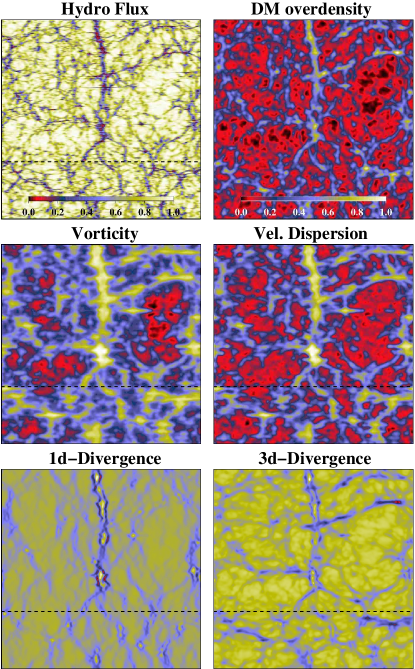
Figure 1: Slices through the Flux (1-dimensionally smoothed at the BOSS resolution) as well as corresponding DM overdensity and velocity fields (3-dimensionally smoothed at 0.5 Mpc/h) in redshift space (horizontal direction). Each field has been extracted from the Horizon-noAGN  simulation at $z=2.5$ and has been normalized to help the visual comparison. The dashed lines correspond to the same line of sight (see Figure 2).

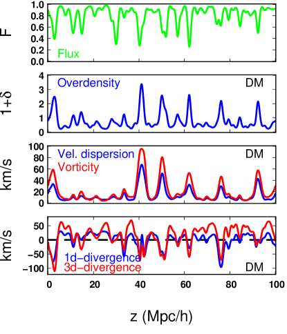
Figure 2: An example showing clear correlations (or anti-correlations) between the evolution of the hydro flux (green line) and DM density and velocity fields (blue and red lines) along the same skewer extracted from the Horizon-noAGN  at $z=2.5$. These skewers are extracted from the slices studied in Fig. 1.

4 Flux and Dark Matter fields

Throughout the present analysis, we have used the Horizon-noAGN  simulation (Peirani et al., 2017) to characterize any relevant cross correlations between the transmitted flux and the different dark matter fields. Horizon-noAGN  is a hydrodynamical simulation of 100 h ^-1Mpc comoving box side run with the RAMSES code (Teyssier, 2002). It evolves 1024³ dark matter particles with a mass resolution of 8.27$\times$10⁷M_⊙ while the initially uniform grid is refined in an adaptive way down to $\Delta x=1$ proper kpc at all times. The simulation adopts a standard $\Lambda$CDM cosmology compatible with WMAP-7 results (Komatsu et al., 2011), namely a total matter density $\Omega_{m}$=0.272, a dark energy density $\Omega_{\Lambda}$=0.728, an amplitude of the matter power spectrum $\sigma_{8}$=0.81, a baryon density $\Omega_{b}$=0.045, a Hubble constant $H_{0}=70.4\,\rm km\,s^{-1}\,Mpc^{-1}$ and n_s=0.967. Horizon-noAGN  is the twin simulation of Horizon-AGN  (Dubois et al., 2014). It contains all relevant physical processes such as metal-dependent cooling, photoionization and heating from a UV background, supernova feedback and metal enrichment, but does not include black hole growth and therefore AGN feedback.

The choice of using Horizon-noAGN  instead of Horizon-AGN  was mainly motivated by the fact that we have performed five additional but slightly lower resolution hydrodynamical simulations to estimate the accuracy and robustness of the LyMAS2 predictions. Thus, turning out the AGN feedback processes in the simulations has permitted us to limit the computational time. These results are presented in appendix A. Furthermore, we have tuned in the present study the UV background intensity in the process of generating the “noAGN” flux grid (see below) in order to get the same mean transmitted Ly-$\alpha$ forest flux $\overline{F}$ derived from Horizon-AGN. By doing this, the flux statistical predictions from the two simulations in the 3d Ly-$\alpha$ clustering tend to be almost the same. This has been already noticed in Lochhaas et al. (2016) when studying the cross-correlations between dark matter haloes and transmitted flux in the Ly-$\alpha$ forest. Note however that AGN feedback is expected to have non negligible effect on the Ly-$\alpha$ 3d clustering such as, for instance, the 1d power spectrum of the Ly-$\alpha$ forest (e.g. Viel et al., 2013; Chabanier et al., 2020).

In the following, we describe briefly how we derived the hydro spectra field and the different DM density and velocity fields from the Horizon-noAGN  simulation. Similarly to P14, we analyse the simulation outputs at redshift $2.5$. Each field is sampled in a regular grid of 1024³ pixels and the size of a single pixel is therefore $\sim$0.1 comoving Mpc/h or 0.04 physical Mpc.

4.1 Transmitted flux

From the Horizon-noAGN, we follow the method to generate the hydro spectra that is fully described in (Peirani et al., 2014). The optical depth of Ly-$\alpha$ absorption is calculated based on the neutral hydrogen density along each line of sight. Basically, the opacity at observer-frame frequency $\nu_{\rm obs}$ is $\tau(\nu_{\rm obs})=\sum_{\rm cells}n_{\mathrm{HI}}\sigma({\nu_{\rm obs}})dl$ where the sum extends over all cells traversed by the line-of-sight, $n_{\mathrm{HI}}$ is the numerical density of neutral H atoms in each cell, $\sigma({\nu_{\mathrm{obs}}})$ is the cross section of Hydrogen to Ly-$\alpha$ photons, and $dl$ is the physical size of the cell. Then each spectrum is smoothed with a 1d Gaussian of dispersion 0.696 h^-1 Mpc, equivalent to BOSS spectral resolution at $z\approx 2.5$. The optical depth along each spectrum is converted to Ly-$\alpha$ forest flux by $F=e^{-\tau}$. Following common practice in Ly$\alpha$ forest modelling, the UV background intensity is chosen to give a mean transmitted Ly-$\alpha$ forest flux $\overline{F}=\langle e^{-\tau}\rangle=$0.795, matching the metal-corrected $z=2.5$ value measured from high-resolution spectra by Faucher-Giguère et al. (2008).

4.2 Density, velocity and mean square velocity

DM skewers that correspond to the “hydro” spectra are also extracted from the hydrodynamical simulation. We use the same 3-step algorithm introduced in P14 to derive both the overdensity, the velocity field and the velocity dispersion fields:

1. adaptive interpolation of the DM particle distribution on a regular grid (Colombi et al., 2007), as detailed in Appendix C;

2. smoothing with a Gaussian window in Fourier space;

3. Extraction of the skewers from a grid of LOS aligned along the $z$-axis.

In step (ii), DM field is three-dimensionally smoothed using different choices of smoothing scales. In P14, we found that a smoothing scale of 0.3 Mpc/h has proved to be optimal leading to the most accurate predictions. However, we prefer a value of 0.5 Mpc/h in the present study since the predictions are very similar to those obtained with 0.3 Mpc/h (see Appendix A). Furthermore, we anticipate with the fact that it is computationally much easier to smooth a DM field to 0.5 Mpc/h than 0.3 Mpc/h when considering large volumes namely with box sides at least greater or equal to 1 Gpc/h.

4.3 Dark matter vorticity

The velocity field is projected (using Cloud-in-Cell interpolations) on a regular grid of resolution 1024 and smoothed over 0.5 Mpc/h with a gaussian filter. The vorticity $\Omega$ is then computed as being the curl of the velocity field using FFT. Slightly smoothing the input velocity field allows us to avoid Gibbs artefacts.

4.4 Dark matter velocity divergence

We have considered both the 3d velocity divergence and the 1d velocity divergence along the line of sight direction.

For the 3d case, we employed two different methods to see whether this could affect our results and trends. The first one is based on a centered finite difference approximation, namely the divergence $\nabla_{3d}^{i}$ at a pixel $i$ is given by

$$\nabla_{3d}^{i}\simeq\frac{V_{x}^{i+1}\!-\!V_{x}^{i-1}}{2h}+\frac{V_{y}^{i+1}\!-\!V_{y}^{i-1}}{2h}+\frac{V_{z}^{i+1}\!-\!V_{z}^{i-1}}{2h},$$ (13)

where $V_{x}^{i}$, $V_{y}^{i}$ and $V_{z}^{i}$ are the velocity components at pixel $i$ and $h$ the size of a pixel (i.e. $100/1024$ Mpc/h here). The second method uses the exact expression of the divergence in Fourier space. However, we found that the two methods lead to very similar results so we will only show results from the Fourier space method for the 3d case.

For the 1d case, we simply use the finite difference approach and the divergence $\nabla_{1d}^{i}$ at a pixel $i$ becomes:

$$\nabla_{1d}^{i}\simeq\frac{V_{z}^{i+1}-V_{z}^{i-1}}{2h}\,,$$ (14)

since we define the $z$-axis as the direction of the LOS.

We summarize in Table 1 the different DM fields used in this study. It is worth mentioning that we changed some of the notations that can be found in P14. We first replaced the definition of the smoothed flux at the BOSS resolution $F_{s}$ in P14 to $F$ here. We also changed the definition of the 3d smoothed DM overdensity, $\rho=1+\delta$ instead of $\Delta_{s}=1+\delta_{s}$ in P14.

Table 1: Summary of fields and corresponding notation used in the text.

Hydro spectra
Flux (smoothed at BOSS res.)	$F$
Optical depth	$\tau$=-ln $F$
Dark Matter Fields
Smoothed density	$\rho_{s}$
Overdensity	$\rho=1+\delta$ = ${\rho_{s}}/{\langle\rho_{s}\rangle}$
Vorticity	$\Omega$
Velocity dispersion	$\sigma$
1d Vel. divergence	$\nabla_{1d}$
3d Vel. divergence	$\nabla_{3d}$

In Fig. 1, we show a slice of the hydro flux (smoothed at BOSS resolution) and the corresponding DM density and velocity fields (smoothed at 0.5 Mpc/h) extracted from the Horizon-noAGN  simulation at redshift 2.5. As expected, clear correlations are noticeable between the transmitted flux and the different DM fields. This trend can also be seen when studying the evolution of each field along the same LOS, and a typical example is given in Fig. 2. We note that high absorptions in the flux correspond to high density regions or high values in the vorticity or the velocity dispersion. But the relative amplitudes of peaks in the density contrast may differ from those of the the velocity dispersion/vorticity. Indeed, the density contrast and the velocicy dispersion/vorticity do not necessary put the emphasis of the same structures (e.g. walls, filaments) as suggested by Fig. 1 or, for instance, by Fig. 2 of Buehlmann & Hahn (2019). On the contrary, these high absorptions rather coincide with high negative values in the 3d or 1d velocity divergence. This is consistent since high density regions are associated with DM haloes in which matter tends to sink toward the center of the objects. Note also that the variations of the modulus of the vorticity and velocity dispersion are very similar.

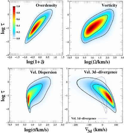
Figure 3: Correlations between the optical depth $\tau=$ -ln$F$ in the hydro spectra (smoothed at the BOSS resolution) and dark matter quantities smoothed at 0.5 Mpc/h namely the overdensity ($1+\delta$), the vorticity ($\Omega$), the velocity dispersion ($\sigma$), the 3d-velocity divergence and the 1d-velocity divergence (along the line of sight) at $z=2.5$. Colors show the density of pixel using normalized values and contour line mark areas enclosing 68.27% and 95.45%. Hydro spectra and DM fields have been computed in redshift space and extracted from the Horizon-noAGN  simulation.

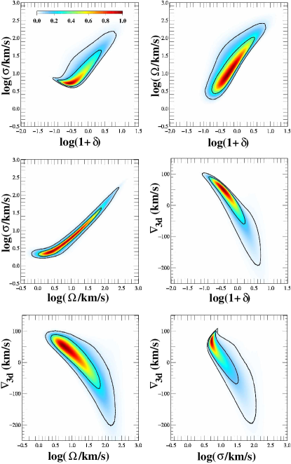
Figure 4: Some correlations between different dark matter quantities from the Horizon-noAGN simulation at $z=2.5$. All field have been smoothed to 0.5 Mpc/h and have been computed in redshift space. Colors show again the density of pixel using normalized values and contour line mark areas enclosing 68.27% and 95.45%.

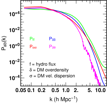
Figure 5: Examples of cross-spectrum $P_{ab}(k)=\langle a^{*}_{k}b_{k}\rangle$ where $a$ and $b$ refer either to the hydro flux or a DM field, derived from the Horizon-noAGN  simulation at $z=2.5$. The flux field is 1d smoothed at the BOSS resolution while the DM field are smoothed at 0.5 Mpc/h.

4.5 Field cross correlations

In order to characterize the correlations that emerge from Figures 1 and 2, we first plot in Fig. 3 some relevant scatter plots between the optical depth $\tau$ and the DM overdensity and velocity fields. The correlations between the optical depth in the hydro spectra and the smoothed DM overdensity (1+$\delta$) is quite similar to the trend found in P14 using the 50 $h^{-1}\,\rm Mpc$ “Horizon MareNostrum” simulation. In Fig. 4, we additionally show the correlations between the different DM fields. As noticed in Fig. 2, the velocity dispersion and vorticity field are highly correlated. We do not show the correlations using the 1d velocity divergence as there are quite similar with trends found using the 3d velocity divergence.

All these plots suggest that there are more or less pronounced correlations between the different input DM fields. It is however tricky to anticipate which combinations of fields through the LyMAS2 scheme would lead to the most accurate theoretical predictions. As specified in section 3, we consider combinations with up to three different DM fields which offers 85 different possibilities (5, 20 and 60 respectively for one, two and three input fields). However, as the main philosophy of LyMAS is to trace the Ly-$\alpha$ flux from the underlying DM distribution with potential corrections from the DM veloctiy field, we will always consider the DM overdensity field in each combination reducing this number to 17. Moreover, since the velocity dispersion and the vorticity fields are highly correlated, we will also always use the velocity dispersion in the 3d case. Consequently, we limit our study to 8 different combinations presented in Table 2. Nevertheless, we have checked that combinations using only DM velocity fields do not lead to satisfactory theoretical predictions.

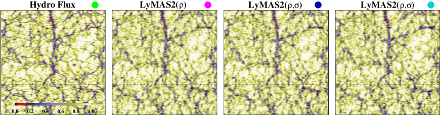
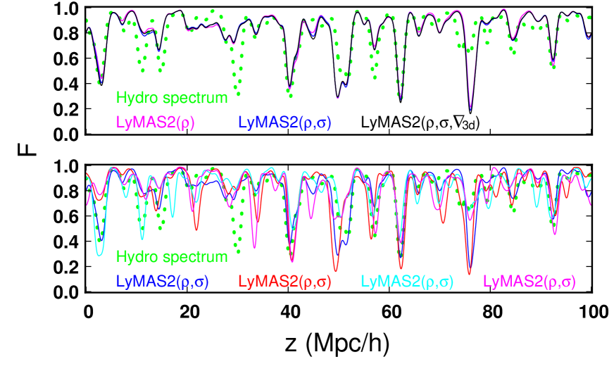
Figure 6: First line: comparison between corresponding slices through the hydro flux (top left panel), 1-dimensionally smoothed at the BOSS resolution, and through pseudo-spectra generated with LyMAS2 and different associations of DM fields (3-dimensionally smoothed at 0.5 Mpc/h). The direction of redshift distorsion is horizontal. Flux and DM fields have been extracted from the Horizon-noAGN  simulation at $z=2.5$. Visual inspection suggests a very good agreement between the clustering of the hydro flux and those of pseudo-spectra. The two bottom panels show the evolution through a specific line of sight (located by the dashed line in the different slices) of the hydro flux (green dotted line) and pseudo-spectra generated with LyMAS2. In the top panel, we use the same seed to randomly generate the covariance from equation (4) for each LyMAS2 realisation. We then note that the difference between the different pseudo-spectra is quite weak. In the bottom panel, we consider LyMAS2($\rho$,$\sigma$) to produce different realisations of pseudo-spectra using this time different seeds to get the covariance. In this case, the difference between pseudo-spectra can be much more pronounced.

Table 2: Summary of the different DM field combinations considered in the LyMAS2 scheme

Name	Field 1	Field 2	Field 3
LyMAS2($\rho$)	Overdens.
LyMAS2($\rho$, $\sigma$)	Overdens.	Vel.disp.
LyMAS2($\rho$, $\Omega$)	Overdens.	Vorticity
LyMAS2($\rho$, $\nabla$1d)	Overdens.	1d div.
LyMAS2($\rho$, $\nabla$3d)	Overdens.	3d div.
LyMAS2($\rho$, $\sigma$, $\Omega$)	Overdens.	Vel.disp.	Vorticity
LyMAS2($\rho$, $\sigma$, $\nabla$1d)	Overdens.	Vel.disp.	1d div.
LyMAS2($\rho$, $\sigma$, $\nabla$3d)	Overdens.	Vel.disp.	3d div.

From each specific association of DM fields, and each Fourier mode $k$ along a LOS, we have estimated the relevant cross-spectra $P_{ab}$ defined in section 3.1, where $a$ and $b$ refer either to the transmitted flux, the DM overdensity or a specific DM scalar field derived from the DM velocity field. For each mode $k$, the covariance matrix $P_{ab}$ is hermitian, and its linear dimension is equal to the total number of fields considered. Examples of cross-power spectra are shown in Fig. 5. We also derived the relevant 1D power spectrum $P_{k}$ required to computed the covariance $\Delta f_{k}$ defined in equation (4). An example of $P_{k}$ is shown in Fig. 16.

5 Creating pseudo-spectra with LyMAS and LyMAS2

In this section, we apply the LyMAS2 scheme to the DM fields extracted from the Horizon-noAGN  simulation to generate grids of pseudo-spectra at BOSS resolution. The objective is to recover the 3d Ly-$\alpha$ clustering statistics of the “true” hydro spectra. For a given skewer, we summarize the main steps to follow to produce a corresponding pseudo-spectrum using either LyMAS or LyMAS2:

The LyMAS scheme:

1. Extract the smoothed overdensity field $\rho$ for a specific skewer.

2. Create a realization $G_{\mathrm{per}}(x)$ of a 1d Gaussian random field from the 1d power spectrum of the Gaussianized percentile spectra derived from the hydro simulation.

3. Degaussianize $g_{\mathrm{per}}(x)=G^{-1}(G_{\mathrm{per}})$ to get a realization of a percentile spectrum.

4. Create a pseudo spectrum by drawing the flux at each pixel from the location in $P(F|\rho)$, implied by the value of $g_{\mathrm{per}}(x)$ (see Eq.6 in P14).

5. One full iteration. We first measure the 1d flux power spectrum $P_{\mathrm{ps}}(k)$ of the pseudo-spectra created in this way. Then we Fourier transform each pseudo-spectrum and multiply each of its Fourier component by the ratio $[P_{\mathrm{F}}(k)/P_{\mathrm{ps}}(k)]^{1/2}$, inverse transform to get the same 1d flux power spectrum than of the true hydro spectra $P_{\mathrm{F}}(k)$ (Weinberg & Cole, 1992). The second step of the full iteration is to compute the PDF of the pseudo-spectra after the 1d Pk re-scaling and then monotonically map the flux value to match the PDF of the true hydro spectra. This full iteration can be repeated several times. However, as we will see, one or two full iterations are enough to get excellent agreement with the 1d power spectrum up to quite high $k$.

The LyMAS2 scheme:

1. Extract and gaussianize the smoothed overdensity field $\rho$ and eventually one or two additional DM velocity fields (e.g. $\sigma$) for a specific skewer.

2. Compute the FFT of each gaussianized field. This gives new (complex) fields, $\rho_{k}$, $\sigma_{k}$, etc..

3. Compute (in Fourier space) the most probable flux $\bar{f_{k}}=T_{1}\cdot\rho_{k}+T_{2}\cdot\sigma_{k}+...$, by applying the relevant filters $T_{1}$, $T_{2}$,$...$ (see for instance equation (12) for the 2-fields case).

4. Generate a 1d Gaussian field of mean 0 and variance defined in equation (4) to get the covariance $\Delta f_{k}$.

5. After computing the inverse Fourier transform of $\bar{f_{k}}+\Delta f_{k}$ to get $f$, degaussianize to get the pseudo-spectrum: $F=G^{-1}(f)$.

6. One full iteration. Same procedure as 4. in the LyMAS scheme.

In Fig. 6, we compare the same slice through the hydro flux and through different realisations of LyMAS2 using different combinations of DM fields. The clustering of each pseudo-spectrum is in fair agreement with the clustering of the hydro spectra. Comparing pseudo-spectra and hydro flux along a specific skewer, also shown in Fig. 6, confirms that LyMAS2 correctly models low and high absorptions at good locations, though amplitudes may differ. The second line of Fig. 6 compares three pseudo-spectra generated with LyMAS2 using three different field combinations but using the same seed for the random process to get the variance $\Delta f_{k}$. It’s interesting to see that these different pseudo-spectra look also the same, which explains why the slices presented in Fig. 6 are very similar. On the contrary, the third line of Fig. 6 shows four different realisations of pseudo-spectrum from LyMAS2 using the DM overdensity and velocity dispersion fields and different seeds to get the covariance $\Delta f_{k}$. In this case, the amplitude of absorptions can be quite different.

In the next sections, we study in more detail the clustering statistics of each catalog of pseudo-spectra produced with LyMAS2. We aim at recovering three observationally relevant statistics of the transmitted flux: the probability density function (PDF), the line-of-sight power spectrum and the 3d clustering (through the 2-point correlation function). As we will see, both LyMAS and LyMAS2 reproduce the PDF of the hydro simulations by construction and nearly reproduce the hydro simulations line-of-sight power spectrum by construction (step 6 above). The power of LyMAS is to produce accurate large-scale 3d clustering while also reproducing these line-of-sight statistics.

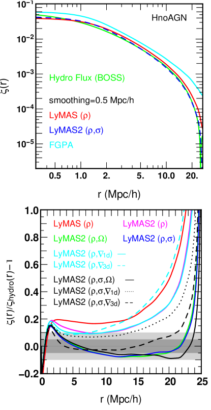
Figure 7: Top panel: the correlation function $\xi$ as a function of the separation $r$. We present results from the true hydro spectra (green line) and results from the LyMAS (red line) and the new version LyMAS2 considering the DM overdensity and the velocity dispersion fields. The predictions from FGPA (cyan line) are also shown. DM fields are all smoothed at the scale 0.5 Mpc/h. Bottom panel: the relative difference as respect to the true hydro spectra (i.e. $\xi(r)/\xi_{\mathrm{hydro}}(r)-1$) are shown for different combination of choices in the Wiener filtering. Here all DM fields have been smoothed to $=0.5$ Mph/h. Compared to the traditional LyMAS scheme (red lines), the new version significantly improves the predictions. In particular the DM overdensity field associated to the DM velocity dispersion (blue line) or the vorticity (green line) leads to relative difference lower than 10% and close to 5% in most of the range we are interested in. On the contrary, using the velocity divergence (cyan lines) does not seem to improve much the results.

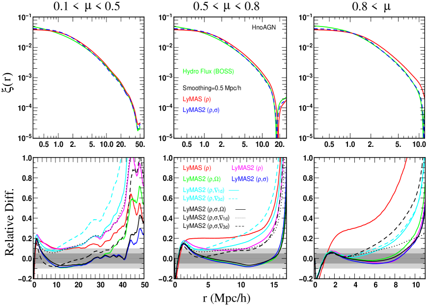
Figure 8: Same as Fig.7 but with a dependency to range of angles $\mu$, as defined in the text. These plots confirm that the association of the DM overdensity and the velocity dispersion (or vorticity) lead to very accurate predictions (see blue or green lines). The corresponding relative differences shown in the bottom panel are generally within 10% and 5% over a wide range of $r$. It is also clear that the new LyMAS2 scheme is much more accurate for large angles where the traditional LyMAS lead to errors that grows quickly with the distance $r$ (red lines). DM fields are again smoothed at $=0.5$ Mph/h.

5.1 3d-clustering

In order to compare the 3d clustering between the hydro and pseudo spectra, we rely on the 2-point correlation function $\xi(r)$ defined by

$$\xi(r)=\frac{\langle F(x)F(x+r)\rangle}{\langle F\rangle^{2}}-1\,,$$ (15)

as a function of the separation ${\bf r}$. To study the effect of redshift distortions, we also consider the 2-point correlation function averaged over bin of angle $\mu$ defined for a pair of pixels ($i$,$j$) by $(r_{i}-r_{j})_{\parallel}/{\bf r}$, where ${\bf r}=|r_{i}-r_{j}|$ and $(r_{i}-r_{j})_{\parallel}$ the component along the line of sight.

The top panel of Fig. 7 shows the full 2-point correlation functions derived from pseudo-spectra using either the first version of LyMAS (red line) or LyMAS2 using the DM overdensity and velocity dispersion field (blue line). Compared to the results of the hydro flux (green line), one can see that LyMAS2 is significantly improving the predictions which are remarkably close to the hydro spectra results. In order to estimate the precision of these reconstructions, we plot in the bottom panel of Fig. 7 the relative difference, i.e. $\xi/\xi_{\mathrm{hydro}}-1$ for different combinations of DM fields. It appears clearly that LyMAS2 leads in general to much more accurate predictions than LyMAS. Indeed, when considering the DM overdensity field only, LyMAS2($\rho$) give slightly better results (magenta line) but the addition of the velocity dispersion lead to errors that are generally lower than 10% and close to 5% (e.g. blue or black lines). Also, similar trends are obtained when the vorticity is taken into account (bottom panel, green line), which is not surprising as these two fields are highly correlated. On the contrary, the 1d and 3d velocity divergence, when associated to the DM overdensity only (cyan lines), do not seem to improve much the predictions as respect to the first version of LyMAS. Note that in linear theory, the 3d velocity divergence is fully correlated with the density field and therefore adds no additional information. On the other hand, the vorticity and/or velocity dispersion are sourced by the non-linear evolution of the matter fields and therefore add complementary information on small scales. Finally, we also note that errors are close to 20% at $r\sim$1-2 Mpc/h probably due to effect of smoothing.

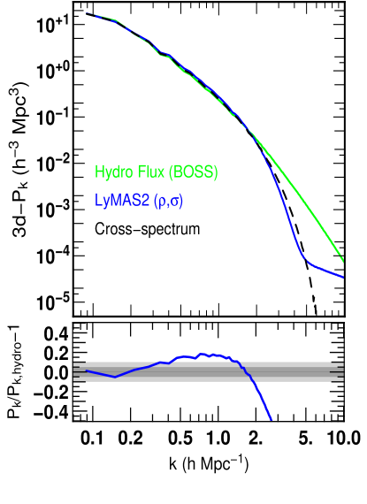
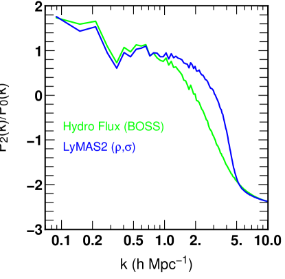
Figure 9: Top panel: the 3d power spectrum derived from the (BOSS) hydro flux (green line) and from pseudo-spectra generated with LyMAS2($\rho$,$\sigma$). All DM fields are smoothed at 0.5 Mpc/h. The black dashed line represents the cross-spectrum. Bottom panel: The corresponding quadrupole to monopole ratios (same color code).

We now investigate how the predictions of the two point correlation functions vary when considering an angle $\mu$. The trends are presented in Fig. 8 for three ranges of values ($0.1<\mu<0.5$, $0.5<\mu<0.8$ and $0.8<\mu$) following P14. The results confirm that LyMAS2 significantly improve the predictions of the Ly-$\alpha$ clustering. In particular, some combinations such as ($\rho$,$\sigma$) still lead to errors generally lower than 10% and most of the time close to 5%. We also note that LyMAS2 is particularly efficient for reproducing the correlations along transverse separations or high angles (i.e. $\mu>$0.8) in which the error is most of the time lower than 5%. The top panels of Fig. 8 indicate again a remarkably good agreement between the 2 point correlation functions of the hydro flux and those derived from pseudo-spectra produced from LyMAS2($\rho$,$\sigma$) even for high angles $\mu>$0.8) where the previous version of LyMAS is quite inaccurate. For the two larget $\mu$ bins, the correlation functions eventually drop rapidly to zero at large $r$. In this regime, the fractional error in $\xi$ are inevitably large, even though the absolute errors are small. It is evident that LyMAS2 captures the scale of these zero-crossing more accurately than LyMAS.

As a first conclusion, the LyMAS2 scheme is significantly improving the predictions of the Ly-$\alpha$ 3d clustering especially when the DM overdensity field is associated with the velocity dispersion or the vorticity field. For the sake of comparison with results presented in the literature, we also compare the 3d power spectrum and corresponding quadropole to monopole ratios in Fig. 9 derived from both the hydro spectra and the pseudo-spectra generated with LyMAS2($\rho$,$\sigma$). The (monopole) power spectrum is defined in the usual way as $\langle\tilde{F}(\mn@boldsymbol{k})\tilde{F}(\mn@boldsymbol{k}^{\prime})\rangle=(2\pi)^{3}P(k)\delta_{\mathrm{D}}(\mn@boldsymbol{k+k}^{\prime})$, with $\tilde{F}(\mn@boldsymbol{k})=\int\mathrm{d}^{3}xF(\mn@boldsymbol{x})\mathrm{e}^{-i\mn@boldsymbol{k.x}}$. Defined this way, we have the following expression of the variance, $\sigma^{2}=\int_{0}^{\infty}k^{3}P(k)\mathrm{dlog}k/(2\pi^{2})$. From Fig. 9, the 3d power spectrum of the hydro spectra can be faithfully recovered from the LyMAS2 simulated spectra up to modes $\sim$2 h Mpc^-1.

For larger modes, however, the predictions are becoming less accurate as separations get lower than the considered smoothing scale (0.5 Mpc/h here). Indeed, we observe a lack of power at small scales (2$\leq$k$\leq$10h Mpc^-1) in the 3d power spectrum of LyMAS2 simulated spectra, compared to the hydro power spectrum, which is mainly explained by the fact that the transverse correlations are not accounted for in the Wiener filtering scheme, and in particular transverse fluctuations at small scales are not generated in the present scheme. On the other hand, the absence of correlation, between the stochastic realisations at small scales for each line of sight, induces an artificial flattening of the reconstructed power spectrum for modes k$\geq$5h Mpc^-1. The ratio of the quadrupole to monopole power is an even stricter test as it traces the anisotropic structure of power in the field, and one can see differences in such a ratio already for modes k$\geq$2h Mpc^-1. This test would clearly benefit from accounting for transverse correlations.

It would be interesting to correct this in a forthcoming work though this point is not critical. Indeed the transverse separations of spectra from existing surveys are generally much larger than 1 Mpc/h, and on these scales the transverse modes are properly reconstructed. Taking into account transverse correlations is straightforward however, and will be worthwile to generalize this method to emission spectra, for which all transverse scales are important. We will therefore include them in future works.

5.2 1d flux power spectrum along LOS

We also aim at producing catalogs of pseudo-spectra that look like spectra measured by a specific instrument i.e. BOSS in the present study. Therefore, the 1d flux power spectrum of each LyMAS mock should be as close as possible to the hydro spectra 1d Pk. In the following, we only present the results derived from LyMAS2($\rho$,$\sigma$) as same trends are obtained when considering any other combination of DM fields. Here, the 1d power spectrum is formally defined as $\langle\hat{F}(k)\hat{F}(k^{\prime})\rangle=(2\pi)P_{\mathrm{1D}}(k)\delta_{\mathrm{D}}(k+k^{\prime})$, where $\hat{F}(k)=\int\mathrm{d}xF(x)\mathrm{e}^{-ikx}$ is the 1d Fourier Transform along the line of sight. When estimating it, we take FFTs along each line of sight and average the result. The expression of the variance is then $\sigma^{2}=\int_{0}^{\infty}kP_{\mathrm{1d}}(k)\mathrm{dlog}(k)/\pi$. Fig. 10 shows the dimensionless 1d power spectrum before power spectrum transformation (red line) and after applying the power spectrum and PDF transformation described in the text (black line). We first note that LyMAS2 without iteration reproduces the 1d power spectrum more accurately than original LyMAS (see Fig.13 of P14). Then as expected, the 1d-$P_{k}$ transformation leads to same power spectrum as the hydro simulation (blue line), by construction. The second step of the iteration is to re-scale the flux PDF, and this transformation slightly alters the 1d power spectrum. However, as illustrated in the bottom part of Fig. 10, the relative difference is close to 2% up to high values of $k$ (i.e $k\sim$2 h Mpc^-1). If one repeats a full iteration a second time, the same accuracy is reached for even higher $k$ values ($\sim$4 h Mpc^-1).

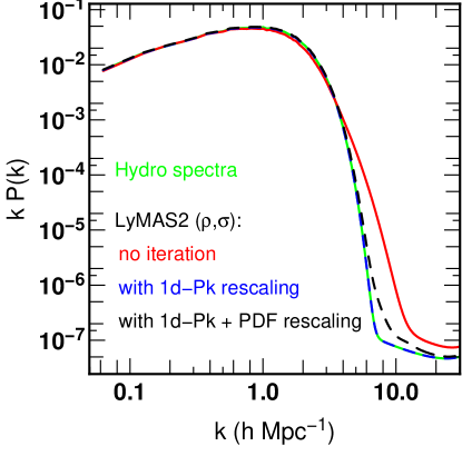
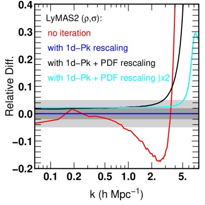
Figure 10: Top panel: the dimensionless 1d power spectrum of the true spectra from the Horizon-noAGN simulation (green line) at $z=2.5$ and from coherent pseudo spectra using LyMAS2 considering the DM overdensity and velocity dispersion fields. We show results before (red line) and after (blue and black lines) 1d power spectrum and PDF transformations (described in the text). Bottom panel: the relative difference as respect to the hydro results (i.e. $P_{k}/P_{k,\mathrm{hydro}}-1$). A full iteration (flux 1d-Pk and PDF re-scaling) permits to recover the hydro power spectrum with an error of $\sim$ 2% over a wide range of $k$. The light and dark grey shaded areas indicate regions where the error is less than 5 and 2% respectively.

5.3 1-point PDF of the Flux

Since the LyMAS scheme ends after a flux PDF re-scaling (second step of a full iteration), this ensures that the 1-point PDF of the hydro flux and the pseudo spectra match exactly. To illustrate, we present in Fig. 11 the results obtained with LyMAS2($\rho$,$\sigma$) before (red line) and after (blue line) a full iteration (1d Pk and PDF re-scaling). Without transformation, the PDF of the pseudo-spectra is already close to the PDF of the hydro spectra (green line). But fractional errors on the PDF can be quite large for low or high values of $F$. After the 1d Pk re-scaling, the PDF of the pseudo-spectra has slightly changed and has some non-physical values ($F<0$ and $F>1$). But the second step of the iteration corrects the PDF (e.g. transforms these unphysical values into physical ones), to exactly match that of the hydro spectra.

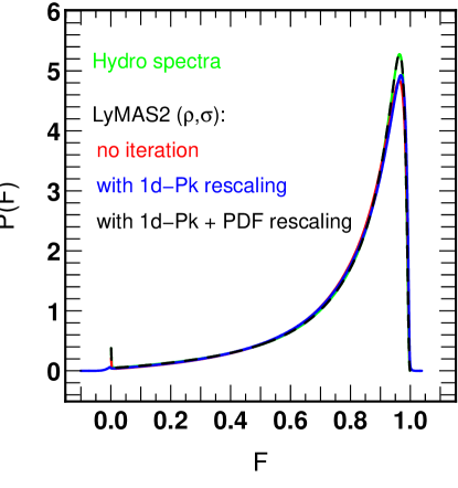
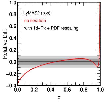
Figure 11: Top panel: the PDF of the true spectra from the Horizon-noAGN simulation at $z=2.5$ (green line) and from coherent pseudo spectra using LyMAS2 considering the DM density and velocity dispersion fields. We show results before (red line) and after (blue and black lines) 1d power spectrum and PDF transformations (described in the text). The 1d Pk re-scaling can lead to non-physical Flux values (i.e. $F<0$ or $F>1$). Bottom panel: the relative difference with respect to the hydro results (i.e. $\mathrm{PDF}/\mathrm{PDF}_{\mathrm{hydro}}-1$). The full scheme permits to recover the hydro flux PDF exactly. The light and dark grey shaded areas indicate regions where the error is less than 10 and 5% respectively.

5.4 Comparison with the FGPA

The FGPA essentially converts DM density to optical depth using a physical model motivated by photoionization equilibrium, assuming that all gas contributing to the Ly-$\alpha$ lies on a temperature-density relation $T\propto(\rho_{s}/\overline{\rho_{s}})^{\gamma-1}$. The predicted flux is:

$$F=Ae^{-(\rho_{s}/\overline{\rho_{s}})^{2-0.7(\gamma-1)}}\,,$$ (16)

where $2-0.7(\gamma-1)\approx 0.6$ for the values of $\gamma$ expected well after reionization (Weinberg et al., 1998; Croft et al., 1998; Peeples et al., 2010; McQuinn, 2009). This relation is reasonable for modeling high-resolution spectra. However, due to existing non-linear relation between flux and optical depth, it does not automatically apply at low resolution (though it omits some physical effects in the high-resolution case). From the Horizon-noAGN  DM overdensity grid smoothed at 0.5 Mpc/h, we have first generated 1024$\times$1024 pseudo-spectra using equation (16) by estimating $A$ so that $\langle F\rangle=0.795$. Then, we one-dimensionally smoothed each pseudo spectrum to BOSS resolution. Similarly to the LyMAS scheme, we end the process by rescaling the flux 1d-Pk and PDF. The correlation function is shown in the top panel of Fig. 7 and is considerably overestimated as respect to the hydro flux with a relative error greater than 50% (omitted in the bottom panel for the sake of clarity). Such a trend is consistent with the results of Sorini et al. (2016) who found that typical relative errors in the 3d power spectrum are $\sim$80% when a DM smoothing scale of 0.4 Mpc/h is considered. In Appendix B, we will investigate other deterministic mapping than the FGPA. But will we see that the main conclusion remains unchanged: deterministic sampling generally tends to significantly overestimate the flux 3d-correlation especially when the dark matter density is smoothed to scales greater than $0.3$Mpc/h. Note that a similar trend is obtained when studying the correlation between the Ly-$\alpha$ transmitted flux and the mass overdensity (see Fig. 1 of Cai et al. (2016)).

5.5 Horizon-AGN VS Horizon-noAGN

In the present work, we used the Horizon-noAGN  simulation for the calibration of LyMAS2, mainly to minimise the computational cost as we derived five additional but lower hydrodynamical simulations to study both the robustness of the results (see appendix A) as well as the effect of cosmic variance (see section 6.2.1). However, since AGN feedback may induce subtle modifications in the spatial distribution and in the clustering of the Ly-$\alpha$ forest, it is important to check if eventual noticeable differences can be seen in the statistics we present so far. For this reason, we have repeated to same and whole analysis but considering this time Horizon-AGN  for the calibration. For instance, we plot in Figure 12 some relevant scatter plots showing the correlations between the optical depth, the DM overdensity and the DM velocity dispersion, similarly to Figures 3 and 4. We also show some transfer functions (i.e. cross-spectrum) that we compare to results from Figure 5. In all cases, the statistics have been derived using a DM smoothing of 0.5 Mpc/h. Compared to results from Horizon-noAGN, we found very similar trends when AGN are included. The comparison of the 2-points correlation function of the hydro flux and LyMAS2($\rho$,$\sigma$) pseudo spectra in Figure 13 confirms this by suggesting predictions with a very similar accuracy when AGN is included or not. In conclusion, the inclusion of galactic winds does not seem to affect significantly the clustering statistics of the Ly-$\alpha$ Forest, given our smoothing scales and targeted accuracy, consistent with results of Bertone & White (2006). Recall that we tuned the UV background in the process of producing the Horizon-noAGN  hydro flux grid, to get the same mean of the Flux. Thus, this conclusion is not surprising and is in agreement with previous finding (Lochhaas et al., 2016). Above all, this means that the predictions of the 3d clustering from the LyMAS2 scheme keep the same accuracy, AGN feedback included or not in the calibration.

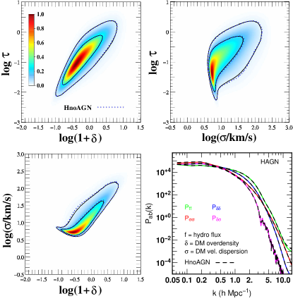
Figure 12: Same as Figs. 3 and 4 but using Horizon-AGN  for the calibration. Here we compare the correlations between the optical depth $\tau=$ -ln$F$ in the hydro spectra (smoothed at the BOSS resolution) and dark matter quantities smoothed at 0.5 Mpc/h namely the overdensity ($1+\delta$) and the velocity dispersion ($\sigma$) at $z=2.5$. We also show in the lower right panel, some relevant transfer functions (i.e. cross-spectrum) similarly to Fig. 5. In all panels, the dotted lines correspond to results from the Horizon-noAGN  simulation. Very similar trends are then obtained when AGN are included or not.

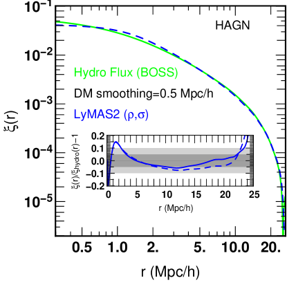
Figure 13: The correlation function $\xi$ as a function of the separation $r$. We present results from the Horizon-AGN  true hydro spectra (green line) and results from LyMAS2 considering the DM overdensity and the velocity dispersion fields (blue dashed line). DM fields are all smoothed at the scale 0.5 Mpc/h. The central small panel indicates the relative difference as respect to the true hydro spectra (i.e. $\xi(r)/\xi_{\mathrm{hydro}}(r)-1$). The blue dashed line represents here the result from the Horizon-noAGN  simulation.

5.6 Influence of redshift distorsions?

Our results indicate that the inclusion of a DM velocity field in LyMAS2, especially the velocity dispersion of the vorticity, clearly improves the predictions of the 3d clustering of the pseudo-spectra. This fact might be understood by the existing correlations between the DM overdensity and the velocity fields (see Fig. 4) and adding a velocity term in the scheme may bring additional information. However, since we also model redshift distortions, this may also introduce or enhance existing correlations between the different considered fields. To estimate the importance of the inclusion of redshift distortion in the process, using Horizon-noAGN, we have repeated the same analysis in real-space i.e. both hydro flux and DM fields have been generated without redshift distortions. Again, we plot in Figure 14 some relevant scatter plots showing the correlation between the optical depth, the DM overdensity and the DM velocity dispersion. We also show some transfer functions (i.e. cross-spectrum). In all cases, the statistics have been still derived using a DM smoothing of 0.5 Mpc/h. Compared to results from Horizon-noAGN  including redshift distortion, the new scatter plots and transfer functions show significant differences, especially when a DM velocity field is considered. The comparison of the 2-points correlation function of the hydro flux and LyMAS2($\rho$,$\sigma$) pseudo spectra in Figure 15 suggests however that errors are still quite low, but a bit higher compared to the relative errors obtained when including redshift distortion. Then, it appears that the inclusion of redshift distorsion seems to slightly improve the predictions of the Ly-$\alpha$ clustering statistics.

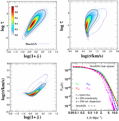
Figure 14: Same as Figs. 3 and 4 but using Horizon-noAGN  without modelling redshift distortions in the LyMAS2 scheme. Here we compare the correlations between the optical depth $\tau=$ -ln$F$ in the hydro spectra (smoothed at the BOSS resolution) and dark matter quantities smoothed at 0.5 Mpc/h namely the overdensity ($1+\delta$) and the velocity dispersion ($\sigma$) at $z=2.5$. We also show in the lower right panel, some relevant transfer functions (i.e. cross-spectrum) similarly to Fig. 5. In all panels, the dotted lines correspond to results from the Horizon-noAGN  simulation with redshift distortions.

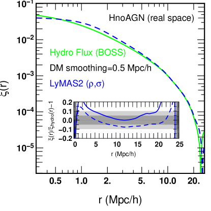
Figure 15: The correlation function $\xi$ as a function of the separation $r$. We present results from the Horizon-noAGN  (NO redshift distortions) true hydro spectra (green line) and results from LyMAS2 considering the DM overdensity and the velocity dispersion fields (blue dashed line). DM fields are all smoothed at the scale 0.5 Mpc/h and are generated in real-space. The central small panel indicates the relative difference as respect to the true hydro spectra (i.e. $\xi(r)/\xi_{\mathrm{hydro}}(r)-1$). The blue dashed line represents here the result from the Horizon-noAGN  simulation including redshift distorsions.

6 Application to large cosmological dark matter simulations

6.1 Simulations of 1.0 and 1.5 Gpc/h box side

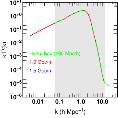
Figure 16: An example of dimensionless 1d Pk required to compute the covariance $\Delta f_{k}$ (see Eq. (4)), derived from the Horizon-noAGN  simulation at $z=2.5$ and considering the overdensity and velocity dispersion in the Wiener filtering (green dashed line). The resolution of the flux and DM grids are 1024³. The red and blue lines are interpolations and extrapolation of the green line to construct the corresponding 1d Pk for larger 1.0 and 1.5 Gpc/h boxes (using grids of resolution 4096³). The grey shaded area indicates the common $k$ range between the 100 Mpc/h and 1 Gpc/h boxes.

In this section we apply our LyMAS2 scheme to large cosmological DM simulations to produce ensembles of BOSS pseudo-spectra. We first ran five cosmological N-body simulations using Gadget2 (Springel, 2005), with a box length of 1.0 Gpc/h with random initial conditions and using the same cosmological parameters as Horizon-noAGN. We additionally run one simulation with a higher volume namely (1.5 Gpc/h)³. As we discuss in detail in section 6.2.2, these latter two values have been chosen to estimate the performances of LyMAS when using DM smoothing scales of 0.5 Mpc/h (fiducial) and 1.0 Mpc/h. respectively In each simulation, the adopted value of the Plummer-equivalent force softening is 5% of the mean inter-particle distance (24.4 kpc/h and 36.6 kpc/h for the 1.0 Gpc/h and 1.5 Gpc/h boxside respectively) and kept constant in comoving units.

From each cosmological simulation, the corresponding DM density and velocity dispersion fields are computed and sampled on grids of 4096³ pixels. This allows us to smooth each 1.0 Gpc/h field to 0.5 Mpc/h and each 1.5 Gpc/h one to 1.0 Mpc/h. According to section 4 and appendix A, the combination of the DM overdensity and velocity dispersion fields leads to accurate and robust Ly-$\alpha$ clustering predictions. We therefore produce our fiducial large BOSS pseudo-spectra with LyMAS2($\rho$,$\sigma$). Note that we choose the velocity dispersion field instead of the vorticity mainly for practical reasons, as the computational and memory costs to compute the latter on a large regular grid is much higher.

Once the different dark matter fields are extracted and smoothed to the appropriate scales, the last inputs we need are the relevant transfer functions $T$ defined in equation (10) whose detailed expressions can be found in equation (11) and equation (12) for the 1d or 2d case respectively. We also need the corresponding 1d power spectrum $P_{k}$ to generate the covariance $\Delta f_{k}$ at the considered box side. Since the calibrations are derived from the Horizon-noAGN  simulation, one potential issue arises from the hydrodynamical box being much smaller than the large DM simulations, so that lower modes are not represented. For the missing modes ($k\leq$2$\pi$/100), we have extrapolated the values of $T_{1}$, $T_{2}$ and $P_{k}$, while in the common $k$ range, we have proceeded with interpolations. As an illustration, Fig. 16 shows the 1d power spectrum required to compute the covariance $\Delta f_{k}$ when considering the DM density and velocity fields extracted from the 100 Mpc/h hydrodynamical simulation as well as the resulting 1d power spectra when considering a 1.0 or 1.5 Gpc/h box side.

Fig. 17 illustrates a reconstruction of pseudo-spectra from a given slice of 4096$\times$4096 pixels through a 1 Gpc/h box simulation. It appears clearly that the 2d clustering of the pseudo-spectra agrees very well with the clustering of the DM overdensity field. Another visual inspection of an individual skewer also shows that peaks of density match with high absorption. It is also interesting to see that the specific skewer shown in Fig. 17 has in its center a large absorption that corresponds to a large and high density region. Note that the study of groups of so called “Coherently Strong Ly-$\alpha$ Absorption” (CoSLA) systems imprinted in the absorption spectra of a number of quasars (from e.g. BOSS) is of particular interest, as they can potentially detect and trace high redshift proto-clusters (see, for instance Francis & Hewett, 1993; Cai et al., 2016; Lee et al., 2018; Shi et al., 2021).

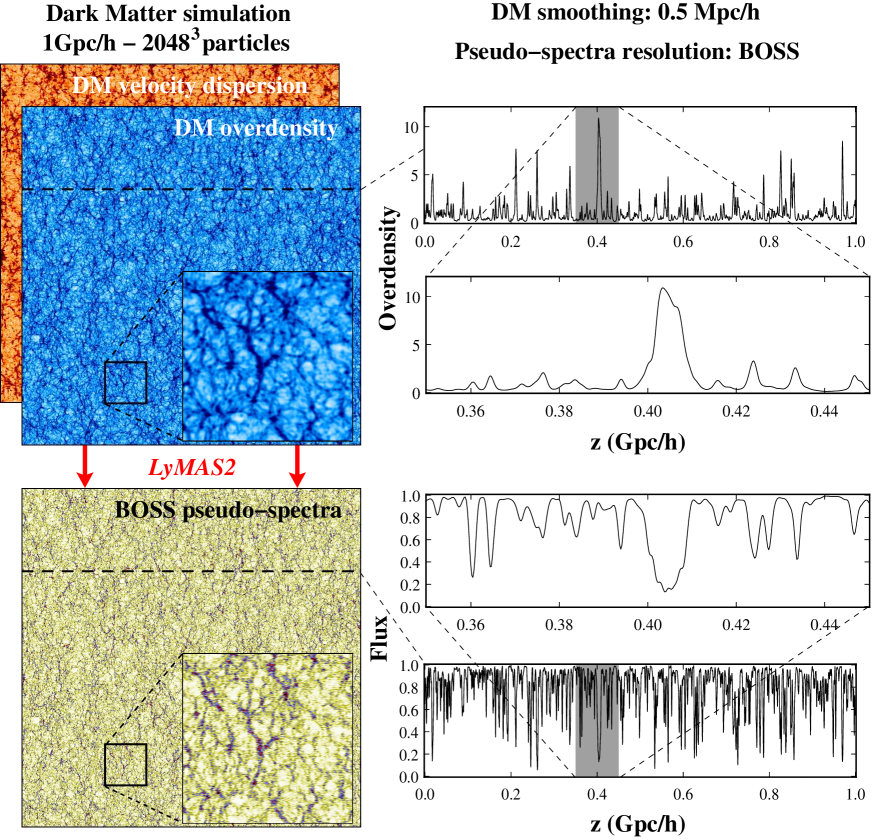
Figure 17: Application of the full LyMAS2 scheme to a large dark matter simulation (1 Gpc/h - 2048³ particles) at $z=2.5$. From the DM overdensity and velocity dispersion fields, both sampled on 4096³ regular grids and smoothed at 0.5 Mpc/h, we derive pseudo-sepctra at the BOSS resolution using the full LyMAS2 scheme. The left part of the figure shows corresponding slices which suggest a fair agreement between the clustering of the DM density and the pseudo spectra. The right part shows an individual skewer confirming that DM density peaks are associated to high flux absorption.

Fig. 18 shows the dimensionless 1d power spectrum of the pseudo-spectra from a 1 Gpc/h simulation before and after iterations. First, in the common $k$-range area between the hydro and the pseudo spectra, we find similar trends to those obtained when applying LyMAS2 to the Horizon-noAGN  simulation (see Fig. 10). For instance, after two full iterations, the relative difference is close to 2% even for high values of $k$ ($\sim$4 h Mpc^-1), and similar results are obtained for the 1.5 Gpc/h pseudo spectra. For lower values of $k$ ($k\leq$2$\pi/100\sim 0.0628$ $h$Mpc^-1), the power spectrum seems to have a natural and consistent extension from the hydro spectra power spectrum. Note also that the highest values of $k$ for the 1.0 and 1.5 Gpc/h box side simulations and grid of resolution 4096³ are respectively 12.87 and 8.58 Mpc^-1, lower than (2$\pi/100)\times 512\sim 32.17$ $h$Mpc^-1 for the hydro box. But the power at these high values is negligible, and missing them in the calculations will not have a noticeable impact on spectra. Also, since a full iteration ends with a Flux PDF re-scaling, this ensures exactly match to the PDF of the hydro flux.

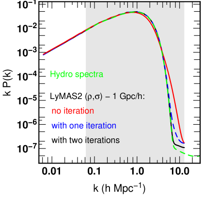
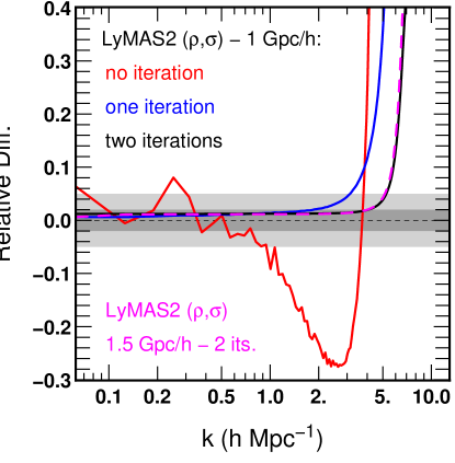
Figure 18: Top panel: the dimensionless, redshift-space, 1d power spectrum of pseudo and true spectra from the Horizon-noAGN simulation (green line) and from coherent pseudo spectra using LyMAS2 considering the DM density and the velocity dispersion fields from a 1 Gpc/h box side N-body simulation. Here again, we show results before (red line) and after (blue line) one full iteration (i.e. flux 1d power spectrum and PDF transformations). We also show the results when repeating a second iteration (black line). The grey shape defines the common k-range between hydro spectra and pseudo-spectra. Bottom panel: the relative difference with respect to the hydro results (i.e. $P_{k}/P_{k,\mathbf{hydro}}-1$). The light grey and dark grey bands define regions where the error is less than 5 and 2 % respectively.

Fig. 19 shows the 2-point correlation functions derived from several large-scale pseudo-spectra. In particular, we show the predictions from the first version of LyMAS (red lines) and those obtained from LyMAS2 using the DM density field only (black lines) and with additional velocity dispersion field (blue lines). We also add the predictions derived from the 1.5 Gpc/h simulation (magenta lines), using again LyMAS2($\rho$,$\sigma$). These plots confirm first that the traditional LyMAS (red lines) tends to overestimate the correlations and this trend is more pronounced when considering high angles ($\mu>0.8$), as already noted in section 4. The result is quite similar with the LyMAS2 scheme when considering the DM overdensity only. However, the difference from LyMAS is more and more noticeable as $\mu$ increases. These results are again consistent with those presented in section 4. The difference becomes even stronger when adding the DM velocity dispersion field. In this case, LyMAS2($\rho$,$\sigma$) tends to significantly reduce the correlations and most probably lead to more reliable predictions. In the range $2\leq r\leq 10$ Mpc/h, the correlations are very close to those of the hydro simulation. It is also impressive that the 1.5 Gpc/h mock generated with LyMAS2($\rho$,$\sigma$) leads to very similar trends (for separations $r\geq 2$ Mpc/h), though the DM fields are now smoothed to 1.0 Mpc/h. This success is consistent with the results presented in the appendix A, where we compare the performance of LyMAS2 using different DM smoothing scales. This robustness is one of the key improvements accomplished with LyMAS2.

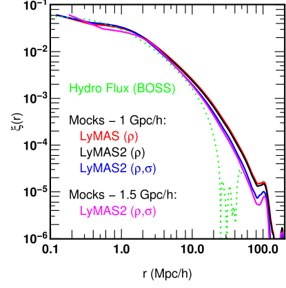
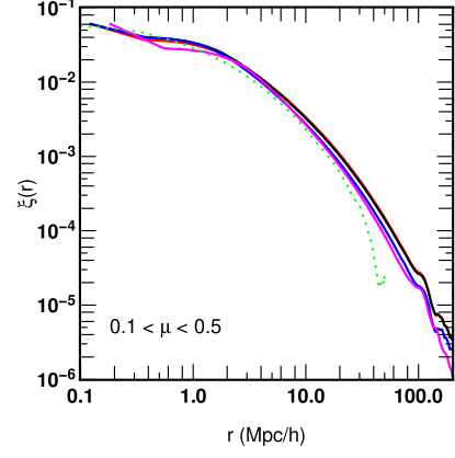
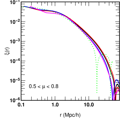
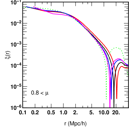
Figure 19: Top left panel: the 2-point correlation functions of the flux derived from the 100 Mpc/h Horizon-noAGN  simulation (green dotted line) and from 1 Gpc/h pseudo-spectra using the full LyMAS (red line) and LyMAS2 scheme using the DM overdensity field only (black line) or combined with the DM velocity field (blue line). We also show the 2-point correlation function derived from 1.5 Gpc/h pseudo spectra produced with LyMAS2($\rho$,$\sigma$) (magenta line). In the other panels, we show the corresponding flux correlation functions averaged over bins of angle $\mu$, as labeled. LyMAS tends to overestimate the correlation especially for large separations and high angles. LyMAS2($\rho$,$\sigma$) tends to significantly reduce such correlations, which suggests more reliable predictions.

Finally, we show in Fig. 20 the 2-point correlation function averaged from five different realizations of 1 Gpc/h Ly-$\alpha$ pseudo-spectra obtained by applying LyMAS2($\rho$,$\sigma$) to different DM cosmological simulations, at $z=2.5$. The plots show clear features of BAO at $r\sim$105 Mpc/h and variations with respect to the angle $\mu$, consistent with observational trends (see for instance du Mas des Bourboux et al. (2020)) This illustrates the ability of LyMAS to properly describe redshift distorsions and to model realistic large BOSS Ly-$\alpha$ forest spectra catalogues.

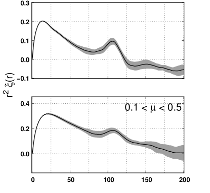
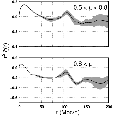
Figure 20: The 2-point correlation function averaged from five different realizations of 1 Gpc/h Ly-$\alpha$ pseudo-spectra obtained by applying LyMAS2($\rho$,$\sigma$) to DM cosmological simulations. Here we use the calibrations obtained from Horizon-noAGN. The shaded areas represent the error on the mean (rms).

6.2 Potential limitations of the method

6.2.1 Effect of cosmic variance?

One potential limitation in the LyMAS scheme is to use an unique hydro simulation to generate the calibration. In other words, we assume this hydro simulation to be fairly representative of the underlying statistics of many simulations which have $\geq$1000 times larger volumes. This makes the resulting large mocks potentially affected by the cosmic variance. In order to estimate this, we have considered our five lower resolution hydro simulations presented in Appendix A, originally produced to estimated the robustness of the LyMAS2 predictions. Here we make good use to estimate the effect of cosmic variance by applying each of the five calibration sets to the (1.5 Gpc/h)³ DM overdensity and velocity grids (of dimension 4096³ each) that we used in section 6.1. In particular, we have computed the 2-point correlation function averaged from these five realizations and shown in Fig. 21. We note that the dispersion tends to be higher for separations between 25 and 100 Mpc/h which makes sense as this corresponds to the scales probed by the reference hydro simulation of box side 100 Mpc/h. We also note that this dispersion tends to be higher for increasing values of the angle $\mu$.

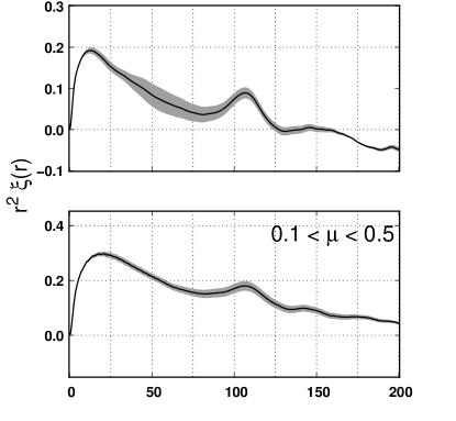
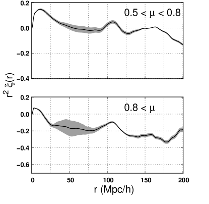
Figure 21: The 2-point correlation function averaged from five different realizations of 1.5 Gpc/h Ly-$\alpha$ pseudo-spectra obtained by applying LyMAS2($\rho$,$\sigma$) to DM cosmological simulations and using five different calibrations. To this regard, we use five lower resolution hydro simulations presented in Appendix A. The shaded areas represent the error on the mean (rms).

6.2.2 Computational limitations

As most of the methods presented in the literature to produce large Ly-$\alpha$ mock catalogs, the LyMAS2 scheme can be divided into two main operations. One the one hand, one needs to generate at a considered smoothing scales, a DM overdensity field and eventually associated velocity fields. This task is generally done using N-body simulations or log normal density fields created from Gaussian initial conditions (e.g. Gnedin & Hui, 1996; Bi & Davidsen, 1997). On the other hand, one has to “paint” the Ly-$\alpha$ absorptions from any los using relevant calibrations or recipes. This latter part is pretty fast in LyMAS since one can treat any los individually and therefore, the algorithm can be easily and optimally parallelized (with openMP for instance). To give an order of magnitude, to create a $\geq$1 Gpc/h box side Ly-$\alpha$ mock presented in section 6.1., using 32 cpu, only $\sim$11 hours are required to generate 4096$\times$4096 BOSS spectra of resolution 4096 and subsequent 1d-Pk and flux PDF rescaling (namely to achieve the six steps of the LyMAS2 scheme presented in section 5). The main limitation of LyMAS2 is however the ability to generate the DM overdensity or a velocity field at the appropriated smoothing scales (i.e. 0.5 and 1.0 Mpc/h in our study). Indeed, the larger the box side of the simulation, the bigger the required dimension of the grid to sample the DM fields. For instance, a simulation box of side 1.0 Gpc/h or 1.5 Gpc/h can be smoothed at the scale of 0.5 Mpc/h and 1.0 Mpc/h respectively if a grid of 4096³ pixels is considered. In these cases, the size of individual pixel is respectively 0.244 and 0.366 Mpc/h which is acceptable, though slightly borderline, to produce the smoothing operation. Moreover, to generate one specific DM field, we used a sophisticated scheme, SmoothDens5, presented in the appendix C. Although SmoothDens5 has been optimized, it needs at least 1 Tb RAM and 50 hours (using 64 cpu) to treat and produce a single DM field, sampled on a regular grid of 4096³, and from a DM simulation using $2048^{3}$ particles.

Technically, it is then rather feasible to generate massive set of mocks if we limit the studied box side to 1.5 Gpc/h. Beyond this value, the computational costs and memory requirement is becoming an issue. It would be definitely worth exploring in near future alternative methods to reduce such costs (e.g. Cell-in-Cloud, …) while not altering the accuracy of the predictions. Moreover, although this is a general issue for all the methods based on DM fields described by N-body simulations, N-body simulations can also become too computationally expensive and time-consuming. Here also alternative methods do exist to obtain the DM fields using cheap approximate methods (e.g. LPT, 2LPT, etc…). However, these are typically not able to produce a very accurate velocity field and this may alter the accuracy of the present LyMAS scheme. Such investigations are beyond the scope of the present paper and will be considered in the next analysis.

7 Conclusions

We have introduced LyMAS2, an improved version of the LyMAS scheme (Peirani et al., 2014). In this new version, we have used the Horizon-noAGN  (Peirani et al., 2017) simulation to characterize the relevant cross-correlations between the transmitted flux and the different DM fields. In particular, we have considered not only the DM overdensity but also specific DM velocity fields (i.e. velocity dispersion, vorticity, 1d and 3d divergence) and used Wiener filtering to generate the specific calibrations. LyMAS2 shares the same philosophy as LyMAS that flux correlations are mainly driven by the correlations of the underlying DM (over)density, and it uses additional information from the DM velocity correlations to refine the theoretical predictions. In a second step, we have applied LyMAS2 to DM fields extracted from the hydrodynamical or large DM-only simulations to create large ensembles of pseudo-spectra with redshift distortions, at $z=2.5$ and at the BOSS resolution. Throughout the analysis, we use a DM smoothing of 0.5 Mpc/h to derive the main trends and results. Our main conclusions can be summarized as follows:

$\bullet$ LyMAS2 greatly improves the predictions for flux statistics of the 3d Ly-$\alpha$ forest on small and large scales. More specifically, we found that the DM overdensity combined with the DM velocity dispersion (or the vorticity) recovers the 2-point correlation functions of the (reference) hydro flux within 10% and (most of the time within 5%) even when high angles are considered. This is a major improvement with respect to the original version of LyMAS, which is rather inaccurate in predicting the Ly-$\alpha$ correlations for large separations and high angles.

$\bullet$ Like LyMAS, LyMAS2 reproduces the 1-point PDF of the flux from the calibrating hydro simulation exactly, by construction. It also reproduces the 1d (line-of-sight) power spectrum with en error of about 2% up high $k$ values. The LyMAS2 pseudo spectra therefore have realistic observable properties on small scales while also having accurate large scale 3d clustering when applied to a large volume DM-only simulation.

$\bullet$ The trends derived from five different and slightly lower resolution hydrodynamical simulations are consistent with those obtained from the fiducial Horizon-noAGN  simulation. This suggests that the results presented in this study are robust. Moreover, this allows us to estimate error bars on the 2-point correlations functions, which are generally low.

$\bullet$ We have considered three different DM smoothing scales (0.3, 0.5 and 1.0 Mpc/h) and found similar trends in the flux clustering predictions. It is encouraging that a DM smoothing of 1.0 Mpc/h still leads to very accurate predictions, especially in the 2-point correlation functions even at high angles and large separation. Indeed, the errors are typically lower than 5%, whereas they are generally higher than 30% with the original version of LyMAS.

$\bullet$ LyMAS2 applied to large DM cosmological simulations of box side either 1.0 or 1.5 Gpc/h indicates that the predicted flux statistics follow the same trends obtained from the (100 Mpc/h) Horizon-noAGN  DM fields. Indeed, we found again that the first version of LyMAS tends to overestimate the flux correlations at large separations and/or at high angles. On the contrary, LyMAS2 using for instance the DM overdensity and the velocity dispersion clearly reduces the 2-point correlation functions to lead to more reliable and accurate predictions. Moreover LyMAS2 adequately models large scale Ly-$\alpha$ absorptions systems which correspond to massive overdensity regions. It is also worth mentioning that these set of mocks were already used to asses the ability to recover the connectivity and clustering properties of critical points of the reconstructed large scale structure from Ly-$\alpha$ tomography in the context of a realistic quasar survey configuration such as WEAVE-QSO (Kraljic et al., 2022).

$\bullet$ Deterministic mappings such as the Fluctuating Gunn-Peterson Approximation tend to considerably overestimate the 3d flux correlations especially at large separation or when high angles are considered.

LyMAS2 offers a sophisticated tool to accurately model and predict large scale Ly-$\alpha$ forest 3d statistics. This opens new opportunities to improve diversified studies such as Ly-$\alpha$ forest cross-correlation (e.g. Lochhaas et al., 2016), two-point correlations or three-point correlations analysis (e.g. Tie et al., 2019) or BAO feature predictions. Moreover, large Ly-$\alpha$ catalogs produced with LyMAS2 can be used to characterize massive overdensity regions such as proto-clusters through groups of coherent large absorptions analysis (Cai et al., 2016; Shi et al., 2021; Lee et al., 2018). Compared to previous work, we recall that the main objective of LyMAS is to create large Ly-$\alpha$ mocks for a specific instrument (here BOSS) with 3d flux statistics as close as possible to those that would be obtained from a very large volume (but computationally intractable) hydrodynamical simulation.

The Iteratively Matched Statistics (IMS) developped by Sorini et al. (2016) does not present such predictions and limits their analysis to small simulation boxes ($\leq$100 Mpc/h). However, when comparing the flux PDF and 1d power spectrum, LyMAS2 and 1D-IMS (see introduction) lead to similar performances: the 1D-IMS scheme perfectly reproduces these statistics, while errors of $\sim$2% are obtained with LyMAS2 for the flux 1d-Pk. Regarding the 3D-IMS scheme, errors are much higher, of order of 15 and 20% respectively for the flux PDF and 1d power spectrum. As far as the 3d flux statistics are concerned, at a DM smoothing of 0.4 Mpc/h, the 1D-IMS and 3D-IMS present errors of 20% and 10-20% (for a DM smoothing of 0.4 Mpc/h) respectively regarding the reconstruction of the power spectrum. In this study, LyMAS2 mainly considers a DM smoothing of 0.5 Mpc/h, which leads to errors generally lower than 5% for the 2-point correlation functions. Again, it is worth mentioning that similar (low) errors are also obtained with LyMAS2 when considering a DM smoothing of 1.0 Mpc/h. It would be then interesting to compare the performance of the 1D and 3D-IMS scheme at this specific smoothing scale in the perspective of creating large ($\geq$ 1.0 Gpc/h) Ly-$\alpha$ mocks.

Recently, Harrington et al. (2021) have trained a convolutional neural network from hydrodynamical simulations of side 20 Mpc/h to predict both the density, the temperature and the velocity fields. This method is quite flexible and the predictions of the flux PDF and 1d power spectrum (i.e. within $\sim$5% up to k$\sim$10 Mpc/h) are promising and more accurate than the FGPA. Note that in a companion paper (Horowitz et al., 2021), convolutional neural networks have also been used to synthesize hydrodynamic fields conditioned on dark matter fields from N-body simulations, which might be very useful for the rapid generation of mocks. Similarly, Sinigaglia et al. (2021) has developed a new physically-motivated supervised machine learning method (HYDRO-BAM) from a reference hydrodynamical simulation of comoving side 100 Mpc/h. The PDF, 3d power spectrum and bi-spectra can be reconstructed with error of a few percent up to modes k$=0.9$ Mpc/h. It would be interesting to see how this promising approach performs when considering smoothed spectra and larger boxes.

Improvements can still be done in the LyMAS scheme. For instance, one main assumption is to consider that the transverse correlations are mainly driven by the effect of DM smoothing. In the present study, we stress again that all the approach is based on creating pseudo-spectra individually and independently from each other. Because the draws of $\Delta f_{k}$ are independent on each line-of-sight, spectra at small but non-zero transverse separations can look quite different on small scales. Since the predictions on the clustering of the flux are already very accurate with LyMAS2, we haven’t considered the same approach in volume. This would take into account transverse correlations between lines of sight that have been neglected in this work: instead of predicting the flux from dark matter fields independently for each LOS, one would predict the entire cube of flux from the dark matter field cubes, using the full 3d covariance structure. One would still use an assumption of spatial homogeneity (stationarity), so that 3d Fourier space coefficients could be computed independently, however one would need to take care of the statistical anisotropy in the LOS direction, therefore all statistics in Fourier space would depend on $|k_{\perp}|$ and $k_{\parallel}$. Taking into account transverse correlations would thus further reduce the covariance of the flux conditionally to the dark matter fields, in other words reduce the noise in the predicted flux field. Among future prospects, we plan to extend this work to predict the flux clustering for other surveys such as the Dark Energy Spectroscopic Instrument (DESI, DESI Collaboration et al., 2016), the William Herschel Telescope Enhanced Area Velocity Explorer (WEAVE-QSO, Pieri et al., 2016) or Subaru Prime Focus Spectrograph (PFS, Takada et al., 2014). They will open new vistas on the high redshift intergalactic medium probed by the Ly-$\alpha$ forest. It would be then interesting to estimate the level of performance of LyMAS2 when the transmitted flux has a higher resolution than BOSS spectra, which might require reducing the DM smoothing. Finally, we also intend to use Machine Learning in the process to see whether we can still improve the predicted flux statistics (Chopitan et al., 2021).

Acknowledgements

We warmly thank the referee for an insightful review that considerably improved the quality of the original manuscript. This work was carried within the framework of the Horizon project (http://www.projet-horizon.fr). Most of the numerical modeling presented here was done on the Horizon cluster at IAP. This work was supported by the Programme National Cosmology et Galaxies (PNCG) of CNRS/INSU with INP and IN2P3, co-funded by CEA and CNES. DW acknowledges support of U.S. National Foundation grant AST-2009735. We warmly thank T. Sousbie, B. Wandelt, O. Hahn, M. Buehlmann and S. Rouberol for stimulating discussions. We also thank D. Munro for freely distributing his Yorick programming language (available at http://yorick.sourceforge.net/) which was used during the course of this work.

Data availability

The data and numerical codes underlying this article were produced by the authors. They will be shared on reasonable request to the corresponding author.

Appendix A General trends

In section 5.1, we have presented the predictions regarding the 2-point correlation functions for eight different combinations of DM fields, with calibrations derived from Horizon-noAGN. To check the robustness of the results, the analysis of other similar hydrodynamical simulations is definitely required. To limit the computational time, we ran five additional hydrodynamical simulations with the same box side and same physics than Horizon-noAGN  but with two times lower resolution (i.e. 512³ DM particles instead of 1024³ and a minimal cell size of $\Delta$x=2 kpc instead of 1 kpc). The first simulation uses degraded Horizon-noAGN  initial conditions while the other ones have different initial phases. For each of the five new simulations, we generated the corresponding grids of transmitted flux, DM overdensity and velocity fields and calibrations folowing the same methodology presented in section 4. We consider here flux and DM fields sampled on grids of 512$\times$512$\times$1024 namely 512$\times$512 spectra of resolution 1024.

In the first step, we consider all DM fields smoothed at 0.5 Mpc/h. After checking first that the “high” and “low” resolution Horizon-noAGN  simulations give consistent trends, we took an interest in the variations of then mean of the absolute relative difference (1/5)$|\sum_{i=1}^{5}$($\xi_{i}/\xi_{hydro,i}$-1)$|$, where we compare the 2-point correlation function of the hydro spectra $\xi_{hydro,i}$ from a given simulation “$i$” to those derived from pseudo-spectra generated with LyMAS2 $\xi_{hydro,i}$. In Fig. 22, we summarize the results obtained with the original LyMAS and LyMAS2 considering the same DM field combinations than in Figures 7 and 8. The main conclusion is that we do find very similar trends than those obtained with Horizon-noAGN  , which strongly suggest that our results are robust. In particular, the use of the velocity dispersion ($\sigma$) or the vorticity ($\Omega$) lead to relative errors that are remarkably low i.e. in general lower than 5% even for the different ranges of angle. The plots also confirm that the 1d and 3d velocity divergence fields do no permit to reach the same level of accuracy.

In the next step, we present the trends obtained when the DM fields are smoothed to 0.3 or 1.0 Mpc/h. We only present in Fig. 23 the results for LyMAS, LyMAS2($\rho$,$\sigma$) and LyMAS2($\rho$,$\sigma$,$\Omega$) to have a clear overview of the general trends. In P14, we found that a DM smoothing of 0.3 Mpc/h was an optimal value to reach the highest accuracy in the predictions. This is confirmed here since we get errors of $\geq$10% compared to $\geq$20% and $\geq$30% with values 0.5 and 1.0 Mpc/h respectively. As expected, LyMAS2 permits to reduces such errors that are in general much lower than 10% and most of the time lower than 5%. It is also very promising that LyMAS2 applied to DM fields smoothed at 1 Mpc/h gives such accurate predictions even for high values of $\mu$. This is definitely not the case with the original LyMAS leading to very high errors. Note also that due the smoothing scale, the predictions are less accurate for distance lower than 2 Mpc/h but acceptable for large scale analysis.

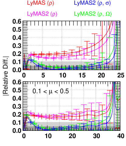
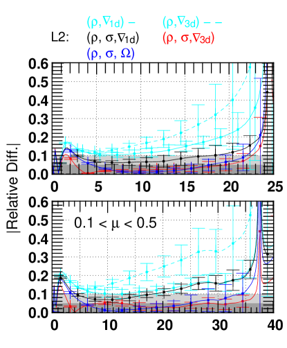
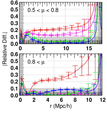
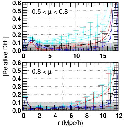
Figure 22: The evolution of the mean of the absolute relative difference in the two point correlation functions (1/5)$|\sum_{i=1}^{5}$($\xi_{i}/\xi_{hydro,i}$-1)$|$ derived from 5 different hydrodynamical simulations at $z=2.5$. All dark matter fields are smoothed to 0.5 Mpc/h. The error bars correspond to the dispersion. Comparison with results from Figures 7 and 8 suggest a very good agreement and therefore robust trends.

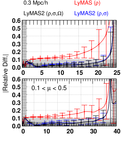
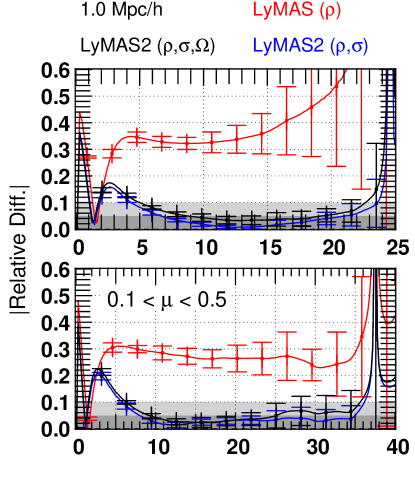
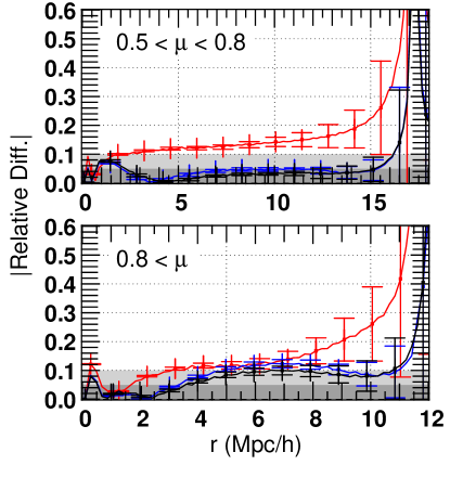
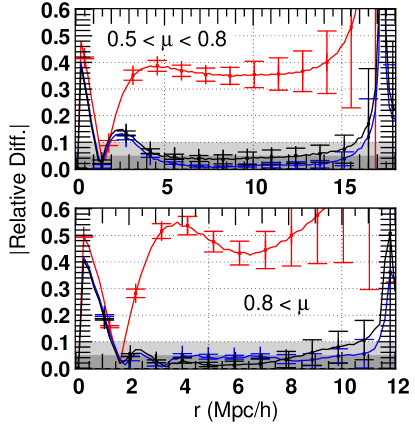
Figure 23: Same as Figure A but for DM smoothing of 0.3 Mpc/h (left column) or 1.0 Mpc/h (righ column). For the sake of clarity, we only show results for the original LyMAS (red curves), LyMAS2($\rho$,$\sigma$) (blue curves) and LyMAS2($\rho$,$\sigma$,$\Omega$) (black curves). Note that even with a DM smoothing of 1.0 Mpc/h, LyMAS2 still permits to reach a high level accuracy, even for high angles ($mu>0.8)$.

Appendix B Deterministic mapping

One commonly way to produce large mocks of Ly-$\alpha$ forest, from Gaussian fields or DM distributions extracted from cosmological simulations, is to use a physically motivated deterministic relation which links the Ly-$\alpha$ optical depth (or transmitted flux) to the dark matter overdensity. This is the case with the so-called Fluctuating Gunn-Peterson Approximation which has been extensively used in the literature. However, the FGPA is supposed to be more suitable for modelling high-resolution spectra and can be strongly limited when the DM density field is smoothed to a scale greater than 0.1 Mpc/h (see for instance the analysis of Sorini et al. (2016)) and confirmed by our results in section 5.4. For this reason, we have derived in P14 an “optimal” deterministic relations by matching the corresponding cumulative distributions of the smoothed transmitted Flux $F_{s}$ and dark matter overdensity $\rho_{s}$ as:

$$\int_{0}^{F_{s}}P(F^{\prime}_{s})dF^{\prime}_{s}=\int_{\rho_{s}}^{\infty}P(\rho^{\prime}_{s})d\rho^{\prime}_{s}\,,$$

where $P(F_{s})$ and $P(\rho_{s})$ are the 1-point PDFs of the flux and DM overdensity measure from the simulation. One advantage of choosing such deterministic relation is to recover by construction the PDF of the hydro flux. However, the 2-point correlation function of pseudo-spectra generated with this approach is still highly overestimated (see for instance Figures 10 and 19 in P14).

In this section, we consider another choices of deterministic relations. In particular, Tie et al. (2019) have used the conditional probability $P(F|1+\delta)$ of the transmitted flux on the DM overdensity to get the conditional mean flux:

$$\overline{F}(1+\delta)=\int F.P(F|1+\delta)dF\,.$$ (17)

It can be analytically demonstrated that the 2-point correlation function of pseudo-spectra obtained from such a determinisic mapping is the same that the one obtained with the first version of LyMAS (Tie et al., 2019). Since this deterministic relation can be easily extended to several DM fields, our aim is to investigate whether the inclusion of different DM velocity fields in such deterministic mappings may improve the trends or not. As an illustration, Fig. 24 shows examples of 1d-deterministic relations constructed for different smoothing of the DM overdensity field and and one example of 2d-deterministic relation $\overline{F}(1+\delta,\sigma)$ using both the DM overdensity and the velocity dispersion fields (smoothed at 0.5 Mpc/h). All relations are derived from the Horizon-noAGN  simulation at $z=2.5$ (in redshift space). In principle, the 2d-deterministic relation is supposed to refine the results as repect to the 1d deterministic one. Indeed, let’s take for instance a DM overdensity of $1+\delta=1$. This leads to an unique mean flux of $\langle F\rangle$=0.75 from the 1d deterministic relation (using a DM smoothing of 0.5 Mpc/h). The 2d-determinisic relation provides, however, a wide range of possible values of $\langle F\rangle$ depending this time on the velocity dispersion (see figure 25).

We have then produced grids of pseudo-spectra from DM fields extracted from the Horizon-noAGN  simulation (see section 4), smoothed at 0.5 Mpc/h and using three different deterministic relations. The first one considers the DM overdensity field only (1-field), the second one both overdensity and velocity dispersion fields (2-fields) while the last one associates the DM density field to the velocity dispersion and vorticity fields (3-fields). To estimate the mean value of the flux from a given value of $\rho$ or a given set of ($\rho$,$\sigma$) or ($\rho$,$\sigma$,$\Omega$), we use respectively interpolations, bilinear interpolations and trilinear interpolations depending of the number of input DM fields. First, Fig. 26 shows the 1d power spectrum and PDF of pseudo spectra (without iteration) for the 2-fields case. We notice that the 1-point PDF is in general not well recovered. The predictions of the 1d-$P_{k}$ are also not as accurate than LyMAS and things especially for the 2-fields and 3-fields cases. Indeed, the power spectra at small scales are considerably overestimated. Although a full iteration can improved these trends, the predicted 2 point correlation functions, shown in Fig. 27, present errors that are generally quite high especially when an angle $\mu$ is considered. For instance the errors are much higher than 10% when $\mu>0.8$.

Also, one main drawback of this approach when creating large mocks ($>$1 Gpc/h) is to have enough statistics from the hydrodynamics simulations to cover most of the parameter space of the large cosmological simulation. This should not be an issue for the 1-field case since simple interpolations and extrapolations can be done (e.g. from Fig. 24 $\langle F\rangle\sim$1 and $\langle F\rangle\sim$0 for $1+\delta<-1.5$ and $1+\delta>1.5$ respectively). For the 2-fields and the 3-fields cases, efficient interpolations and extrapolations could be obviously much more complicated to realized.

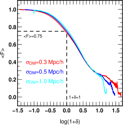
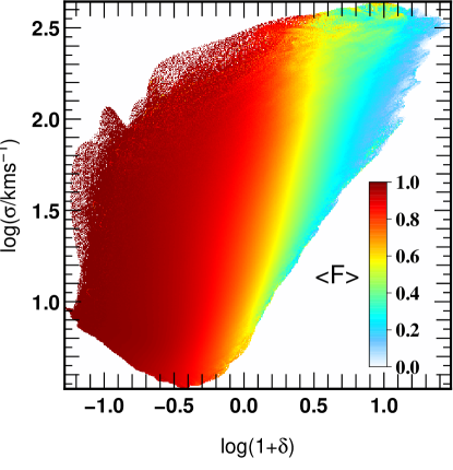
Figure 24: Examples of 1d and 2d deterministic relations derived from the Horizon-noAGN  simulation at $z=2.5$. Top panel: The mean flux $<F>$ only depends on the DM overdensity $1+\delta$. Three different DM smoothing have been considered. For example, the mean flux has a value of 0.75 for an overdensity of 1 (DM smoothing$=$0.5 Mpc/h). Bottom panel: scatter plot showing the mean flux $<F>$ as respect to the DM overdensity and velocity dispersion field ($\sigma$). In this case, $<F>$ can have a wide range of values for $1+\delta$=1 (see also Figure 25).

Figure 25: The evolution of the mean flux as respect to the velocity dispersion ($\sigma$) and for a given overdensity (i.e. $1+\delta$=1). The DM fields are smoothed at 0.5 Mpc/h. This variation is directly derived from the 2d deterministic sampling presented in Figure 24. Compared to the 1d deterministic relation, a wide range of values of $<F>$ is obtained and should refine the predictions.

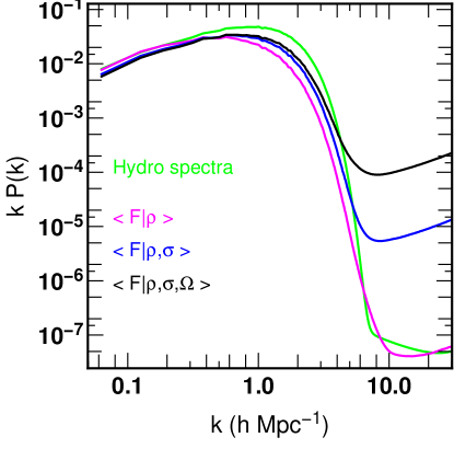
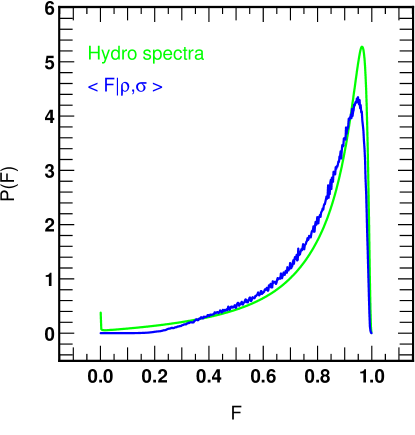
Figure 26: Top panel: the 1d power spectrum of pseudo spectra generate from Horizon-noAGN  DM fields (smoothed at 0.5 Mpc/h; $z=2.5$) and using deterministic relations described in the text. The discrepancies with the hydro 1d-Pk are quite pronounced especially at small scales. Bottom panel: an example of PDF of pseudo-spectra compare to hydro spectra, showing again a noticeable disagreement. All results are presented without a full iteration in the scheme (flux 1d-Pk and PDF rescaling).

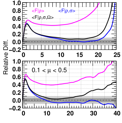
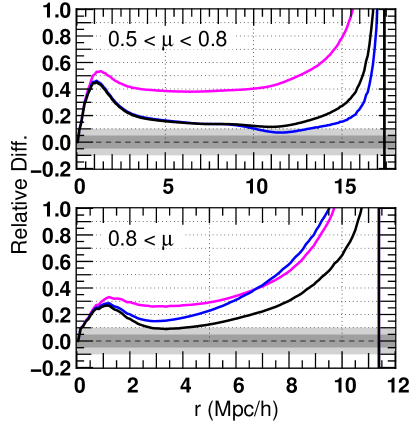
Figure 27: The relative difference of the two-point correlation functions of pseudo-spectra produced with deterministic sampling (and a full iteration in the scheme). It appears clearly that the different deterministic sampling do no reach the level of accuracy of LyMAS2 especially for high angles where the error are quite high ($>10\%$). The light and dark grey shade represent error lower that (absolute) 10 and 5% respectively.

Appendix C Adaptive smoothing

In this section we provide some detail on how the dark matter density field, velocity field and velocity dispersion are interpolated adaptively on a mesh from the output of a cosmological dark matter $N$-body simulation, before further treatment by LyMAS2, in particular additional smoothing with a Gaussian window.

Note that, while the notations below assume standard configuration space, the calculation naturally extend to redshift space, by just modifying particle coordinates accordingly with the local peculiar velocity component contribution. In LyMAS2, we use the infinitely remote observer approximation by just accounting for redshift distortion along $z$ axis.

For a smooth phase-space distribution function $f(\mn@boldsymbol{x},\mn@boldsymbol{v})$, the projected density is given by

$$\rho_{\rm E}(\mn@boldsymbol{x})=\int{\rm d}^{3}v\,f(\mn@boldsymbol{x},\mn@boldsymbol{v}),$$ (18)

the Eulerian mean velocity field by

$$\mn@boldsymbol{v}_{\rm E}(\mn@boldsymbol{x})=\langle\mn@boldsymbol{v}\rangle_{\rm E}=\frac{1}{\rho_{\rm E}(\mn@boldsymbol{x})}\int{\rm d}^{3}v\,\mn@boldsymbol{v}\,f(\mn@boldsymbol{x},\mn@boldsymbol{v}),$$ (19)

and the local mean square velocity reads

$$\langle v^{2}\rangle_{\rm E}(\mn@boldsymbol{x})=\frac{1}{\rho_{\rm E}(\mn@boldsymbol{x})}\int{\rm d}^{3}v\,v^{2}\,f(\mn@boldsymbol{x},\mn@boldsymbol{v}).$$ (20)

Obviously, the last two equations stand for points of space where $\rho(\mn@boldsymbol{x})>0$. From equation (20), we can derive the local velocity dispersion

$$\sigma_{v,{\rm E}}^{2}\equiv\langle v^{2}\rangle_{\rm E}-v_{\rm E}^{2}.$$ (21)

We notice that the local velocity field can be considered as a statistical average, this is why we used the $\langle\cdots\rangle_{\rm E}$ notation above,

$$\langle\mn@boldsymbol{v}\rangle_{\rm E}(\mn@boldsymbol{x})=\int{\rm d}^{3}v\,\mn@boldsymbol{v}\,f_{\rm E}(\mn@boldsymbol{x},\mn@boldsymbol{v}),$$ (22)

with the local density probability

$$f_{\rm E}(\mn@boldsymbol{x},\mn@boldsymbol{v})\equiv\frac{1}{\rho_{\rm E}(\mn@boldsymbol{x})}f(\mn@boldsymbol{x},\mn@boldsymbol{v}).$$ (23)

In this probabilistic approach, the mean square velocity is given by equation (20), since

$$\langle v^{2}\rangle_{\rm E}(\mn@boldsymbol{x})=\int{\rm d}^{3}v\,v^{2}\,f_{\rm E}(\mn@boldsymbol{x},\mn@boldsymbol{v}).$$ (24)

and, likewise, its local variance by equation (21).

What we have actually access to is not a smooth distribution function, unfortunately, but a distribution of $N$ simulation particles of individual masses $m_{i}$, positions $\mn@boldsymbol{x}_{i}$ and velocities $\mn@boldsymbol{v}_{i}$. This means that the phase-space distribution function has the following form

$$f(\mn@boldsymbol{x},\mn@boldsymbol{v})=\sum_{i}m_{i}\,\delta_{\rm D}(\mn@boldsymbol{v}-\mn@boldsymbol{v}_{i})\,\delta_{\rm D}(\mn@boldsymbol{x}-\mn@boldsymbol{x}_{i}),$$ (25)

where $\delta_{\rm D}$ is the Dirac distribution function. From eq. (25), one can compute the projected Eulerian density

$$\rho_{\rm E}(\mn@boldsymbol{x})=\sum_{i}m_{i}\,\delta_{\rm D}(\mn@boldsymbol{x}-\mn@boldsymbol{x}_{i}),$$ (26)

but the Eulerian velocity field $\mn@boldsymbol{v}_{\rm E}(\mn@boldsymbol{x})$ and mean square velocity are ill-defined.

However, the underlying distribution of true dark matter particles is much smoother than its crude numerical representation in terms of macroparticles of the $N$-body simulation. While, strictly speaking, the phase-space density is still of the form (25) at the microscopic level, it can be considered as a smooth function at the macroscopic level, at least in terms of probability density.

In order to recover a good approximation of the continuum, Colombi et al. (2007) proposed a locally adaptive smoothing algorithm, SmoothDens, inspired from smooth particle hydrodynamics (hereafter SPH), using, to compute various fiels, an interpolation window $F_{\mn@boldsymbol{x}}$, of which the shape parameters, in particular the typical size $\ell(\mn@boldsymbol{x})$, depend on position $\mn@boldsymbol{x}$. This window function is normalized to unity, i.e. $\int{\rm d}^{3}x^{\prime}\,F_{\mn@boldsymbol{x}}(\mn@boldsymbol{x}^{\prime})=1$.

In principle, for a given function $h(\mn@boldsymbol{x},\mn@boldsymbol{v})$, the smoothed counterpart is given by

$$[F_{\mn@boldsymbol{x}}*h](\mn@boldsymbol{x},\mn@boldsymbol{v})=\int{\rm d}^{3}x^{\prime}\,F_{\mn@boldsymbol{x}}(\mn@boldsymbol{x}-\mn@boldsymbol{x}^{\prime})\,h(\mn@boldsymbol{x}^{\prime},\mn@boldsymbol{v}).$$ (27)

Setting $h=\rho_{\rm E}$, after simple algebraic calculations exploiting the properties of the Dirac distribution function, we obtain the simple expression for the adaptively smoothed density:

$$\rho_{\rm F}(\mn@boldsymbol{x})=\sum_{i}m_{i}\,F_{\mn@boldsymbol{x}}(\mn@boldsymbol{x}-\mn@boldsymbol{x}_{i}).$$ (28)

From there, we can formally define the analogous of equation (23) but with adaptive smoothing performed in the spatial position,

$$f_{\rm F}(\mn@boldsymbol{x},\mn@boldsymbol{v})\equiv\frac{1}{\rho_{\rm F}(\mn@boldsymbol{x})}[F_{\mn@boldsymbol{x}}*f](\mn@boldsymbol{x},\mn@boldsymbol{v}),$$ (29)

from which one can derive estimates in the mean field limit of velocity related quantities:

$$\mn@boldsymbol{v}_{\rm F}(\mn@boldsymbol{x})=\frac{\sum_{i}m_{i}\,\mn@boldsymbol{v}_{i}\,F_{\mn@boldsymbol{x}}(\mn@boldsymbol{x}-\mn@boldsymbol{x}_{i})}{\sum_{i}m_{i}\,F_{\mn@boldsymbol{x}}(\mn@boldsymbol{x}-\mn@boldsymbol{x}_{i})},$$ (30)

$${\langle v^{2}\rangle}_{\rm G}=\frac{\sum_{i}m_{i}\,v^{2}_{i}\,F_{\mn@boldsymbol{x}}(\mn@boldsymbol{x}-\mn@boldsymbol{x}_{i})}{\sum_{i}m_{i}\,F_{\mn@boldsymbol{x}}(\mn@boldsymbol{x}-\mn@boldsymbol{x}_{i})}.$$ (31)

In the algorithm SmoothDens, the adaptive procedure is used to compute various fields for a particular set of positions $\mn@boldsymbol{x}=\mn@boldsymbol{x}_{j}$ on a cubical grid of size $n_{\rm g}$. Function $F$ is a compact Monaghan & Lattanzio (1985) spline of size $\ell(\mn@boldsymbol{x})$, with $\ell(\mn@boldsymbol{x})$ the distance of the $N_{\rm SPH}^{\rm th}$ closest simulation particle to position $\mn@boldsymbol{x}$. The value of $N_{\rm SPH}$ we adopt here is $N_{\rm SPH}=32$. As an additional recipe, adaptive smoothing is locally replaced with nearest grid point (NGP) interpolation (Hockney & Eastwood, 1988) when $\ell(\mn@boldsymbol{x})$ is smaller or of the order of the grid cell size $L/n_{\rm g}$, where $L$ is the simulation box size. Also, a local weight is given to each particle $i$ so that at the end, its total contribution sums up to the particle mass $m_{i}$. Note that, due to the finite extension of the spline function, some particles belonging to dense clusters or close to dense clusters may not contribute at all. In the latest implementation of the algorithm, SmoothDens5, which we use in LyMAS2, an option allows one to affect these particles to the grid with NGP interpolation in order to conserve total mass. The effect of not doing so is however generally small.

The outcome of SmoothDens mainly depends on two parameters, the resolution $n_{\rm g}$ of the grid and the value used for the number of neighbors, $N_{\rm SPH}$. Changing both these parameters can have drastic impact on the results, especially the local velocity dispersion and the velocity derivatives estimates. Additional Gaussian smoothing performed in LyMAS2 is however expected to reduce considerably the dependence on these two parameters provided that the smoothing scale $R_{\rm G}$ associated to the smoothing window is large enough compared to $L/n_{\rm g}$. Yet one has to bear in mind that the influence of $N_{\rm SPH}$ cannot be negligible in underdense regions as long as it can influence scales larger than $R_{\rm G}$, which is unfortunately very likely. Despite these non trivial issues, the reason why LyMAS2 still works so accurately is that it is calibrated relying on probability distributions mappings, which naturally corrects for intrinsic biases introduced by local adaptive smoothing.

References

- Bautista et al. (2017) Bautista J. E., et al., 2017, A&A, 603, A12
- Bertone & White (2006) Bertone S., White S. D. M., 2006, MNRAS, 367, 247
- Bi & Davidsen (1997) Bi H., Davidsen A. F., 1997, ApJ, 479, 523
- Blanton et al. (2017) Blanton M. R., et al., 2017, AJ, 154, 28
- Bolton et al. (2017) Bolton J. S., Puchwein E., Sijacki D., Haehnelt M. G., Kim T.-S., Meiksin A., Regan J. A., Viel M., 2017, MNRAS, 464, 897
- Buehlmann & Hahn (2019) Buehlmann M., Hahn O., 2019, MNRAS, 487, 228
- Busca et al. (2013) Busca N. G., et al., 2013, A&A, 552, A96
- Cai et al. (2016) Cai Z., et al., 2016, ApJ, 833, 135
- Caucci et al. (2008) Caucci S., Colombi S., Pichon C., Rollinde E., Petitjean P., Sousbie T., 2008, MNRAS, 386, 211
- Chabanier et al. (2020) Chabanier S., Bournaud F., Dubois Y., Palanque-Delabrouille N., Yèche C., Armengaud E., Peirani S., Beckmann R., 2020, MNRAS, 495, 1825
- Chopitan et al. (2021) Chopitan N., Lavaux G., Peirani S., 2021, in prep
- Colombi et al. (2007) Colombi S., Chodorowski M. J., Teyssier R., 2007, MNRAS, 375, 348
- Croft et al. (1998) Croft R. A. C., Weinberg D. H., Katz N., Hernquist L., 1998, ApJ, 495, 44
- Croft et al. (1999) Croft R. A. C., Weinberg D. H., Pettini M., Hernquist L., Katz N., 1999, ApJ, 520, 1
- DESI Collaboration et al. (2016) DESI Collaboration et al., 2016, arXiv e-prints, p. arXiv:1611.00036
- Dalton et al. (2016) Dalton G., et al., 2016, in Evans C. J., Simard L., Takami H., eds, Society of Photo-Optical Instrumentation Engineers (SPIE) Conference Series Vol. 9908, Ground-based and Airborne Instrumentation for Astronomy VI. p. 99081G, doi:10.1117/12.2231078
- Dalton et al. (2020) Dalton G., et al., 2020, in Society of Photo-Optical Instrumentation Engineers (SPIE) Conference Series. p. 1144714, doi:10.1117/12.2561067
- Dawson et al. (2013) Dawson K. S., et al., 2013, AJ, 145, 10
- Dawson et al. (2016) Dawson K. S., et al., 2016, AJ, 151, 44
- Delubac et al. (2015) Delubac T., et al., 2015, A&A, 574, A59
- Dubois et al. (2014) Dubois Y., et al., 2014, MNRAS, 444, 1453
- Eisenstein et al. (2011) Eisenstein D. J., et al., 2011, AJ, 142, 72
- Faucher-Giguère et al. (2008) Faucher-Giguère C.-A., Prochaska J. X., Lidz A., Hernquist L., Zaldarriaga M., 2008, ApJ, 681, 831
- Font-Ribera et al. (2012) Font-Ribera A., et al., 2012, J. Cosmology Astropart. Phys., 2012, 059
- Font-Ribera et al. (2013) Font-Ribera A., et al., 2013, J. Cosmology Astropart. Phys., 2013, 018
- Font-Ribera et al. (2014) Font-Ribera A., et al., 2014, J. Cosmology Astropart. Phys., 2014, 027
- Francis & Hewett (1993) Francis P. J., Hewett P. C., 1993, AJ, 105, 1633
- Gnedin & Hui (1996) Gnedin N. Y., Hui L., 1996, ApJ, 472, L73
- Harrington et al. (2021) Harrington P., Mustafa M., Dornfest M., Horowitz B., Lukić Z., 2021, arXiv e-prints, p. arXiv:2106.12662
- Hockney & Eastwood (1988) Hockney R. W., Eastwood J. W., 1988, Computer simulation using particles
- Horowitz et al. (2021) Horowitz B., Dornfest M., Lukić Z., Harrington P., 2021, arXiv e-prints, p. arXiv:2106.12675
- Japelj et al. (2019) Japelj J., et al., 2019, A&A, 632, A94
- Komatsu et al. (2011) Komatsu E., et al., 2011, ApJS, 192, 18
- Kraljic et al. (2022) Kraljic K., et al., 2022, arXiv e-prints, p. arXiv:2201.02606
- Lee et al. (2015) Lee K.-G., et al., 2015, ApJ, 799, 196
- Lee et al. (2018) Lee K.-G., et al., 2018, ApJS, 237, 31
- Lochhaas et al. (2016) Lochhaas C., et al., 2016, MNRAS, 461, 4353
- Lynds (1971) Lynds R., 1971, ApJ, 164, L73
- McQuinn (2009) McQuinn M., 2009, ApJ, 704, L89
- Monaghan & Lattanzio (1985) Monaghan J. J., Lattanzio J. C., 1985, A&A, 149, 135
- Ozbek et al. (2016) Ozbek M., Croft R. A. C., Khandai N., 2016, MNRAS, 456, 3610
- Palanque-Delabrouille et al. (2013) Palanque-Delabrouille N., et al., 2013, A&A, 559, A85
- Peeples et al. (2010) Peeples M. S., Weinberg D. H., Davé R., Fardal M. A., Katz N., 2010, MNRAS, 404, 1281
- Peirani et al. (2014) Peirani S., Weinberg D. H., Colombi S., Blaizot J., Dubois Y., Pichon C., 2014, ApJ, 784, 11
- Peirani et al. (2017) Peirani S., et al., 2017, MNRAS, 472, 2153
- Pichon et al. (2001) Pichon C., Vergely J. L., Rollinde E., Colombi S., Petitjean P., 2001, MNRAS, 326, 597
- Pieri et al. (2016) Pieri M. M., et al., 2016, in Reylé C., Richard J., Cambrésy L., Deleuil M., Pécontal E., Tresse L., Vauglin I., eds, SF2A-2016: Proceedings of the Annual meeting of the French Society of Astronomy and Astrophysics. pp 259–266 (arXiv:1611.09388)
- Ravoux et al. (2020) Ravoux C., et al., 2020, J. Cosmology Astropart. Phys., 2020, 010
- Sargent et al. (1980) Sargent W. L. W., Young P. J., Boksenberg A., Tytler D., 1980, ApJS, 42, 41
- Schaye et al. (2015) Schaye J., et al., 2015, MNRAS, 446, 521
- Shi et al. (2021) Shi D., Cai Z., Fan X., Zheng X., Huang Y.-H., Xu J., 2021, arXiv e-prints, p. arXiv:2105.02248
- Sinigaglia et al. (2021) Sinigaglia F., Kitaura F.-S., Balaguera-Antolínez A., Shimizu I., Nagamine K., Sánchez-Benavente M., Ata M., 2021, arXiv e-prints, p. arXiv:2107.07917
- Slosar et al. (2011) Slosar A., et al., 2011, J. Cosmology Astropart. Phys., 2011, 001
- Slosar et al. (2013) Slosar A., et al., 2013, J. Cosmology Astropart. Phys., 2013, 026
- Sorini et al. (2016) Sorini D., Oñorbe J., Lukić Z., Hennawi J. F., 2016, ApJ, 827, 97
- Springel (2005) Springel V., 2005, MNRAS, 364, 1105
- Takada et al. (2014) Takada M., et al., 2014, PASJ, 66, R1
- Teyssier (2002) Teyssier R., 2002, A&A, 385, 337
- Tie et al. (2019) Tie S. S., Weinberg D. H., Martini P., Zhu W., Peirani S., Suarez T., Colombi S., 2019, MNRAS, 487, 5346
- Viel et al. (2013) Viel M., Schaye J., Booth C. M., 2013, MNRAS, 429, 1734
- Vogelsberger et al. (2014) Vogelsberger M., et al., 2014, MNRAS, 444, 1518
- Weinberg & Cole (1992) Weinberg D. H., Cole S., 1992, MNRAS, 259, 652
- Weinberg et al. (1997) Weinberg D. H., Hernsquit L., Katz N., Croft R., Miralda-Escudé J., 1997, in Petitjean P., Charlot S., eds, Structure and Evolution of the Intergalactic Medium from QSO Absorption Line System. p. 133 (arXiv:astro-ph/9709303)
- Weinberg et al. (1998) Weinberg D. H., Katz N., Hernquist L., 1998, in Woodward C. E., Shull J. M., Thronson Harley A. J., eds, Astronomical Society of the Pacific Conference Series Vol. 148, Origins. p. 21 (arXiv:astro-ph/9708213)
- du Mas des Bourboux et al. (2020) du Mas des Bourboux H., et al., 2020, ApJ, 901, 153