Compact extra dimensions as the source of
primordial black holes

Abstract

We discuss the model of the primordial black holes formation at the reheating stage. These small massive black holes appear due to specific properties of the compact extra dimensions. The latter gives rise the low energy model containing the effective scalar field potential capable for the domain walls production. Formed during inflation, these walls are quite dense so they collapse soon after inflation ends. The discussion is performed within the scope of multidimensional $f(R)$-gravity.

Keywords extra dimensions, modified gravity, $f(R)$-gravity, primordial black holes, cosmology, domain wall.

1 Introduction

Extra dimensions are usually studied within the framework of elementary particle physics [1], for example in the context of the unification of interactions [2, 3], explaining the nature of the Standard Model fields [4], searching for their manifestations in collider experiments [5, 6]. This paper explores another possible cosmological consequence — shows that compact extra dimensions may be the cause of the primordial black holes (PBHs) formation immediately after the end of the inflation.

It is known that one of the central tasks of theories with compact extra dimensions is to provide their compactification and stabilization [7] during cosmological evolution. This can be done, for example, by introducing additional scalar fields [8] or $f(R)$-modification of gravity [9, 10]. The latter approach is particularly promising because the Starobinsky quadratic $f(R)$-gravity [11, 12] gives the best fit to observational constraints on the parameters of the inflation [13]. Moreover, in multidimensional $f(R)$-gravity, the processes of cosmological inflation and compactification are manifestations of general gravitational dynamics in different subspaces [14].

The possibilities of $f(R)$-gravity are widely studied [15, 16], they offer solutions to many cosmological problems [17, 18, 19, 20]. One of the problems that $f(R)$-gravity can solve is the existence of primordial black holes. Today, the primordial origin of some discovered black holes (quasars at small $z$ [21, 22], BHs of intermediate masses detected by gravitational-wave observatories [23]) is hotly discussed [24, 25, 26]. In this paper we demonstrate how the primordial black holes can appear as a result of inflationary dynamics in the framework of $f(R)$-gravity model.

The idea of our proposed mechanism is based on the known possibility of domain walls formation during cosmological inflation followed by their collapse into primordial black holes [27, 28]. The formation of such domain walls requires a scalar field with a nontrivial potential containing several vacuums. Such kind of scalar field effectively arises in the multidimensional $f(R)$-models in the Einstein frame [29, 10, 14]. This field controls the size of the compact extra space, and its different vacuums correspond to different universes. In this paper we calculate the parameters of the domain walls formed by the field and conclude that appearing at inflationary stage they will immediately collapse into PBHs during reheating. For a remote observer in the Jordan frame the appearance of such PBH is interpreted as a manifestation of non-trivial $f(R)$-gravitational dynamics of multidimensional space. These formed PBHs will grow rapidly in the process of further cosmological evolution due to accretion and are capable to turn into observable supermassive quasars at small $z$.

2 Model

The study is based on the modified $f(R)$ gravity acting in $D=4+n$ dimensions. It is described by the action

$$S=\frac{m_{D}^{D-2}}{2}\int d^{4+n}x\sqrt{|g_{D}|}\,\left[f(R)+c_{1}R_{AB}R^{AB}+c_{2}R_{ABCD}R^{ABCD}\right]\,,$$

$$f(R)=a_{2}R^{2}+R-2\Lambda_{D}\,,$$ (1)

where $m_{D}$ is the multidimensional Planck mass. The parameters $a_{2},c_{1},c_{2}$ of the Lagrangian (2) have dimensionality $[m_{D}^{-2}]$, the cosmological constant $\Lambda$ has dimensionality $[m_{D}^{2}]$. Hereafter we will work everywhere in units $m_{D}\equiv 1$, unless it is explicitly specified. In this work we will represent multidimensional space as the direct product of $\mathbb{M}=\mathbb{M}_{4}\times\mathbb{M}_{n}$, where $\mathbb{M}_{4}$ is– four-dimensional space, $\mathbb{M}_{n}$ – an $n$-dim compact extra space with metric

$$ds^{2}=g_{\mu\nu}dx^{\mu}dx^{\nu}-e^{2\beta(t,x)}d\Omega^{2}_{n}\,.$$ (2)

Here $g_{\mu\nu}$ is a 4-dimensional metric $\mathbb{M}_{4}$, $\beta$ is a metric function and $d\Omega^{2}_{n}$ is the linear element square of a maximally symmetric compact extra space $\mathbb{M}_{n}$ with positive curvature.

Cosmological scenarios based on this theory [29, 14, 30]. are finished by an effective 4-dim theory at the low energy. Its properties are defined by the Lagrangian parameters of of action (2). The procedure for obtaining such a theory is also described in [10].

Following this procedure, we assume maximal symmetry of the extra space $\mathbb{M}_{n}$. Its radius $\rho\equiv e^{\beta}$ does not depend on the extra coordinates. In addition, the useful approximation of this effective theory works in a region where the extra curvature $R_{n}=n(n-1)/e^{2\beta}$ is large compared to the 4-dimensional curvature and changes slowly:

$$R=R_{4}+R_{n}+P_{k}\,,\quad P_{k}=2n\,\partial^{2}\beta+n(n+1)(\partial\beta)^{2}\,,$$

$$R_{4},P_{k}\ll R_{n}\,.$$ (3)

where $R_{4},R_{n}$ are Ricci scalars for $\mathbb{M}_{4},\mathbb{M}_{n}$. The approximation (3) applied to action (2) leads to the effective 4-dim model with a non-minimal coupling between the observed 4-dimensional gravity $R_{4}$ and the scalar field [10]. Therefore the resulting theory will be written in the Jordan frame and we will use this frame as the physically observed one [31].

3 Effective scalar field action

The minimal coupling between the observed 4-dimensional gravity and the scalar field is achieved by the transition to the Einstein frame, which strongly facilitate the analysis. This transition has been performed in detail in [10], [32]:

$$S=\frac{m_{4}^{2}}{2}\int d^{4}x\sqrt{-g_{4}}\ \text{sign}(f^{\prime})\left[R_{4}+K(\phi)(\partial\phi)^{2}-2V(\phi)\right]\,,$$ (4)

where the Planck mass in the Einstein frame is $m_{4}=\sqrt{2\pi^{\frac{n+1}{2}}/\Gamma(\frac{n+1}{2})}$, and $g_{4}^{\mu\nu}$ is the observed 4-dimensional metric. The Ricci scalar of the extra space is perceived as the scalar field, $\phi\equiv R_{n}$.

The action (4) contains a potential and a nontrivial kinetic term, which are expressed through the initial parameters of the Lagrangian (2) (see [14]):

$$K(\phi)=\frac{1}{4\phi^{2}}\left[6\phi^{2}\left(\frac{f^{\prime\prime}}{f^{\prime}}\right)^{2}-2n\phi\left(\frac{f^{\prime\prime}}{f^{\prime}}\right)+\frac{n(n+2)}{2}\right]+\frac{c_{1}+c_{2}}{f^{\prime}\phi}\,,$$ (5)

$$V(\phi)=-\frac{\operatorname{sign}\left(f^{\prime}\right)}{2(f^{\prime})^{2}}\left[\frac{|\phi|}{n(n-1)}\right]^{n/2}\left[f(\phi)+\frac{c_{1}+2c_{2}/(n-1)}{n}\phi^{2}\right]\,.$$ (6)

The transition validity from (2) to (4) dictated by ineaqualities (3) will be analyzed later.

For a wide range of parameters, the potential term (6) has two minima corresponding to different vacuums of the Universe (Fig. 1). The value of the potential at these minima must be almost zero according to almost zero value of the cosmological constant $\Lambda_{4}$. It leads to a relation of the parameter $c=1/4(a+c_{v}/n)$, where $c_{v}=c_{1}+2c_{2}/(n-1)$.

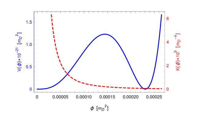
Figure 1: Graphs of the potential term and kinetic factor (5), (6) for parameters: $n=6$, $c_{1}=-8000$, $c_{2}=-5000$, $a_{2}=-500$. The left minimum of the potential is at $\phi=0$, but it is impossible to roll down to it in a finite time because of the increasing friction effect of the kinetic factor, the right minimum is at $\phi_{min}=2.3\cdot 10^{-4}.$

The rolling of the field $\phi\equiv R_{n}$ into the right minimum of the potential (6) corresponds to the stabilization of the compact extra space $R_{n}\neq 0$ (the extra space is compactified and has some radius $\rho_{0}$), and leads to the observed cosmology [14]. The presence of the left minimum $R_{n}\approx 0$ suggests the possibility of another scenario [30], in which the extra space is unstable and expands to macroscopic scale.

The non-trivial kinetic factor (5) significantly modifies the character of the field evolution $\phi(t)$ in comparison to the standard scalar-field theory, providing an increasing friction when rolling to the left minimum, see Fig. 1. One can simplify the Lagrangian by substituting

$$\psi=m_{4}\int\limits_{\phi_{0}}^{\phi}\sqrt{K(\phi^{\prime})}\,d\phi^{\prime}\,,\quad\tilde{V}(\psi)=m_{4}^{2}\,V(\phi(\psi)),\quad K(\phi^{\prime})>0\,.$$ (7)

In this case, $\psi(\phi)$ is monotonic and invertible (which is required to find the potential in the expression (8)). After simple algebra, the Lagrangian is reduced to the standard form

$$S=\frac{m_{4}^{2}}{2}\int d^{4}x\sqrt{-g_{4}}\,R_{4}+\int d^{4}x\sqrt{-g_{4}}\,\left[\frac{1}{2}(\partial\psi)^{2}-\tilde{V}(\psi)\right]\,,$$ (8)

where $m_{4}^{2}=16\pi^{3}/{15}$ for chosen extra space dimensionality $n=6$.

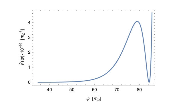
Figure 2: Graph of the potential term $\tilde{V}(\psi)$ of the effective theory (8) for the parameters chosen in Fig. 1. The right minimum is at $\psi_{min}=84.3$. Strictly speaking, the left minimum is at $\psi=-\infty$, but for our purposes a very accurate approximation $\psi=0$ is sufficient (corresponding to $\phi=\phi_{0}$), up to which the effective theory (4) still works. The maximum value of the potential in the transition region between vacuums $\tilde{V}_{max}\approx 4.1\cdot 10^{-20}$ and the steepness of the slope $\sqrt{\tilde{V}^{\prime\prime}(\psi_{max})}=2.7\cdot 10^{-11}$.

4 Domain walls

It is well known that potentials like (2), containing several minima (vacuums), can lead to formation of non-trivial field configurations [33] — "bubbles" of one vacuum inside another, surrounded by a domain wall.

Let us investigate such a configuration by deriving the field equation for $\psi$ from the effective action (8). For simplicity, we consider it spherically symmetric and static, which gives the equation:

$$\psi_{uu}+\frac{2\psi_{u}}{u}-\tilde{V}^{\prime}(\psi)=0\,,$$ (9)

where $u$ is the radial coordinate. When considering a sufficiently large "bubble" (such that its radius is much larger than the characteristic thickness of the domain wall $\psi_{uu}\gg 2\psi_{u}/u$) it can easily be reduced to a first-order equation

$$\partial_{u}\psi=\pm\sqrt{2\tilde{V}(\psi)}\,.$$ (10)

The characteristic solution of the equation (10) connecting the left vacuum of the potential $\tilde{V}(\psi)$ to the right one (Fig. 2) is shown in Fig. 3 (blue line).

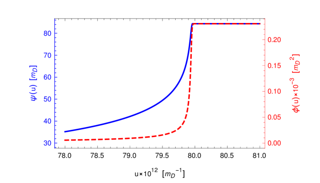
Figure 3: Numerical solution of (9) under boundary conditions: the left minimum $\tilde{V}(\psi)$ (Fig. 2) is reached inside the bubble $\psi(0)=0$, and the right minimum is reached for the remote observer $\psi(u\rightarrow\infty)=\psi_{min}$ (and forms our Universe). In the graphs: the blue line is the direct solution of $\psi(u)$ (domain wall) and the red dashed line is its corresponding function $\phi(u)$. In this example the bubble radius is $u_{0}\approx 8\cdot 10^{13}$.

We can calculate the domain wall energy density $\varepsilon_{\psi}$ as a component $T^{00}$ of energy-momentum tensor for the scalar field Lagrangian $\psi$:

$$\varepsilon_{\psi}(u)=T^{00}(u)=\cfrac{\partial\mathcal{L}_{\psi}}{\partial\left(\partial_{0}\psi\right)}\,\partial^{0}\psi-\mathcal{L}_{\psi}g^{00}=\frac{1}{2}(\partial_{u}\psi)^{2}+V(\psi)=2\tilde{V}(\psi(u)).$$ (11)

Integration over the radial coordinate (11) gives the surface energy density of the domain wall in multidimensional Planck units ($m_{D}=1$):

$$\sigma=\int\limits_{0}^{\infty}\varepsilon_{\psi}(u)\,du=\int\limits_{0}^{\psi_{min}}\frac{2\tilde{V}(\psi)}{\psi_{u}}\,d\psi=\int\limits_{0}^{\psi_{min}}\sqrt{2\tilde{V}(\psi)}\,d\psi\,.$$ (12)

We can also formally estimate the characteristic wall thickness $\delta$ as

$$\sigma= \int\limits_{0}^{\infty}2\tilde{V}(\psi)\,du\approx 2\frac{\tilde{V}_{max}}{2}\,\delta\quad\implies\quad\delta\approx\frac{\sigma}{\tilde{V}_{max}}\,.$$ (13)

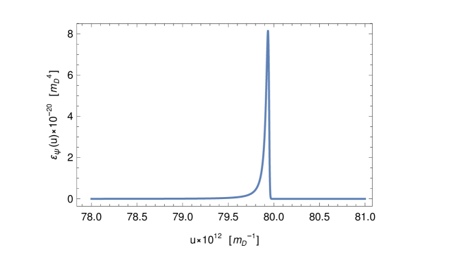
Figure 4: Energy density (11) profile along the radial coordinate $u$ for the solution shown in Fig. 3. In the case of spherical symmetry, the domain wall forms a bubble with surface energy density $\sigma\approx 5\cdot 10^{-9}$ and wall thickness $\delta\approx 1.2\cdot 10^{11}$, according to (12), (13).

Domain walls considered in this paper appears to be very massive (Fig. 4). As a result, they could be a source of primordial black holes. The mechanism of formation and collapse of such domain walls is well studied in [34, 35, 27] and leads to the formation of primordial black holes in a wide range of masses.

5 Generation of domain walls during inflation

As stated above, the rolling of the $\psi$ field to the right minimum of Fig. 2, creates the observable Universe. For its formation, a mechanism of the cosmological inflation is required. In order not to complicate our consideration, we will consider the inflation as an external process with a characteristic Hubble parameter $H$.

The mechanism of inflationary production of the bubbles of alternative vacuum is well known [27]. As a result of repeated quantum fluctuations, the field $\psi$ can be flipped from the region of rolling down to the right minimum to the region of rolling down to the left minimum in some area of the inflationary Universe. Thy size of this region is growing during inflation while the $\psi$ field is frozen near the potential maximum. After the end of inflation, the field tends to one minimum inside the bubble and another minimum outside it. Increasing energy density gradually forms the domain wall (Fig. 4) around the bubble.

Several constraints must be imposed on the working model of domain wall production in the considered $f(R)$-gravity:

1. During cosmological inflation, 4-dimensional space is described by a de Sitter metric with curvature $R_{4}\simeq 12H^{2}$, where $H$ is the Hubble parameter. Therefore, the approximation (3) is applicable only for field values $\phi\equiv R_{n}\gg R_{4}\simeq 12H^{2}$. From Fig. 1 we see that $\phi\sim 10^{-6}-10^{-4}$, so to satisfy the constraint we need $H\ll 10^{-4}$.

2. To generate walls via quantum fluctuations of field $\psi$ (near the maximum of potential 2) its slow rolling is required: $\sqrt{\tilde{V}^{\prime\prime}(\psi_{max})}\ll H$. According to Fig. 2 we see that $\sqrt{\tilde{V}^{\prime\prime}(\psi_{max})}\sim 10^{-11}$, so to satisfy the constraint we need $H\gg 10^{-11}$.

3. Domain walls should not be too dense so as not to dominate the inflaton: $\varepsilon_{\psi}\ll\varepsilon_{inf}\sim H^{2}m_{4}^{2}$. From Fig. 4 we see that $\varepsilon_{\psi}\sim 10^{-20}$, so to satisfy the constraint we need $H\gg 10^{-11}$.

4. The fluctuations of the $\psi$ field during inflation should not be too large to prevent overproduction of the domain walls: $\delta\psi=H/2\pi\ll\psi$. As one can see from Fig. 2, $\psi\sim 10$, so to satisfy the constraint we need $H\ll 10$.

All constraints above are satisfied if the inflation has the characteristic scale $10^{-11}\ll H\ll 10^{-4}$. Here $m_{4}=5.75$ for $n=6$ according to (4). Remind that all estimations are given in the Einstein frame and if the dimensionality is not explicitly specified, all calculations are carried out in $m_{D}\equiv 1$ units.

In the previous sections, all calculations were performed in the Einstein frame. As a physically observable one it is often accepted to consider the Jordan frame, in which it is possible to manipulate the 4-dimensional Planck scale $M_{4}=\Omega(\phi_{\text{min}})m_{4}$ by adjusting the size of extra space. So we will transform final physical results to the Jordan frame. Cosmological inflation should be described in a physically observable frame — that is the Jordan frame (let’s denote it by the index $J$):

$$S^{J}_{\text{inf}}=\int d^{4}x\sqrt{-g_{4}^{J}}\,\left[\frac{1}{2}\left(\partial\chi^{J}\right)^{2}-U^{J}\left(\chi^{J}\right)\right]\,,$$ (14)

where $\chi$ is the inflaton whose potential $U(\chi)$ determines the Hubble parameter $H\sim\sqrt{G\,U(\chi)}$ during the inflation. The constraint above on $H$ have been checked for the inflation in the Einstein frame (denote it by the index $E$). The transition to it from (14) is known [36, 14]:

$$g_{\mu\nu}^{J}=\Omega^{-2}g_{\mu\nu}^{E}\,,\quad\text{where}\quad\Omega^{2}=e^{n\beta(\phi)}|f^{\prime}(\phi)|.$$ (15)

Substituting (15) into (14), we obtain the action written in Einstein frame:

$$S^{J}_{\text{inf}} =\int d^{4}x\sqrt{-g_{4}^{E}}\,\left[\frac{1}{2}\Omega^{-2}\left(\partial\chi^{J}\right)^{2}-\Omega^{-4}U^{J}\left(\chi^{J}\right)\right]\approx$$

$$\approx\int d^{4}x\sqrt{-g_{4}^{E}}\,\left[\frac{1}{2}\left(\partial\chi^{E}\right)^{2}-U^{E}\left(\chi^{E}\right)\right]=S^{E}_{\text{inf}}\,,$$ (16)

where transformations of the inflaton $\chi^{E}=\Omega^{-1}\chi^{J}$ and its potential $U^{E}=\Omega^{-4}U^{J}$ to the Einstein frame are made. Here we use the fact that during inflation the field $\phi$ is practically frozen (constraint 2) and is in the region of maximum of potential, so the factor $\Omega(\phi)$ can be considered constant and equal $\Omega\approx\Omega(\phi_{\text{max}})\sim\Omega(\phi_{\text{min}})\sim 10^{8}$ for the parameters chosen in Fig. 1.

The Hubble parameter for the inflaton $\chi^{E}$ observed in the Einstein frame is related to the Hubble parameter for the $\chi^{J}$ inflaton observed in the Jordan frame as follows:

$$H^{E}\sim\sqrt{G\,U^{E}(\chi)}=\sqrt{G\ \Omega^{-4}U^{J}(\chi)}\sim\Omega^{-2}H^{J}\,.$$ (17)

From this, in accordance with the constraint for $H$ obtained above for the Einstein frame, it follows that $H^{J}>10^{5}\sim 10^{-4}\ [M_{4}]\sim 10^{14}\ [\text{GeV}]$ at the chosen parameters. It is consistent with the observed data [13].

6 Formation of primordial black holes

During the inflationary stage the classical motion of the scalar field $\psi$ is frozen — this is determined by the constraint 2 in Section 5). If there a seed for the future domain wall appear during quantum fluctuations (the field jumps to the left slope of the potential in Figure 2), then in this place the field values $\psi$ should lie near the potential maximum since the fluctuations are small (constraint 4 in Section 5). At the end of inflation, the inflaton the Hubble parameter vanishes and the $\psi$ field begins to rapidly roll from the maximum to the potential minima (to the left minimum, for the inner region of the bubble and to the right minimum for the outer region). During this roll-off, the energy density $\sigma(t)$ in the transition region gradually grows up to the value $\sigma$ calculated in the previous sections. In addition, due to postinflationary expansion, the radius of the region is growing $u_{w}(t)=u_{0}a(t)$ also, where $u_{0}$ is radius at the end of inflation and $a(t)$ is scale factor. Because of this, the mass of the formed domain wall increases $m_{w}(t)=4\pi u_{w}(t)^{2}\sigma(t)$ together with its gravitational radius $u_{g}(t)=2Gm_{w}(t)$. At a certain time, the gravitational radius will cross the entire domain wall $u_{g}(t_{*})=u_{w}(t_{*})$ and a primordial black hole with mass $m_{w}(t_{*})$ will form for a remote observer.

The moment $t_{*}$ of crossing of the wall by the gravitational radius in our model will come long before it reaches the final energy density $\sigma$. This can be seen from the fact that the ratio of the gravitational radius to the size of the wall (assuming that the wall has a final energy density $\sigma$) is grater than unity

$$\frac{u_{g}}{u_{w}}=8\pi G\sigma u_{w}>m_{4}^{-2}\sigma\delta\approx 16\,,$$ (18)

where the fact that the wall radius is always larger than its thickness $u_{w}(t)>\delta$ is used. The ratio (18) is calculated for the wall parameters obtained in Fig. 4 and holds for any model parameters (1) satisfying the set of constraints discussed in Section 5. Therefore, the wall is formed long before the field rolls to the potential minima. The black hole is formed at the time $t_{*}$ when the horizon radius $u_{g}$ is approximately equal to the wall radius $u_{w}$. Hence, the mass of the PBH can be estimated as

$$M_{PBH}\simeq m_{w}(t_{*})\simeq u_{g}(t_{*})/2G\simeq u_{w}(t_{*})/2G\equiv u_{0}a(t_{*})/2G\,.$$ (19)

All processes described above occur in a very short time interval $t_{*}$, which is significantly less than the characteristic time of the field $\psi$ roll-off to the minimum of potential, $t_{*}<\tau_{\psi}\sim\sqrt{V^{\prime\prime}(\psi_{\text{max}})}^{-1}\sim 10^{6}$. This time in our model is less than the inflation time $\tau_{\text{inf}}\approx 60\ H^{-1}\sim 10^{7}$. Therefore, the roll-off of field $\psi$ process occurs at the reheating stage (as for the inflaton), the scale factor at which we can approximately [37] consider $a(t_{*})=\left((\tau_{\text{inf}}+t_{*})/\tau_{\text{inf}}\right)^{\frac{\nu+2}{3\nu}}<\left((\tau_{\text{inf}}+\tau_{\psi})/\tau_{\text{inf}}\right)^{\frac{\nu+2}{3\nu}}\sim\left(1+10^{-1}\right)^{\frac{\nu+2}{3\nu}}\sim 1$, where $\nu$ is the index of degree in the inflaton potential. It means that the time interval $t_{*}$ is very short and one can neglect the post-inflationary expansion.

The radius $u_{0}$ is determined by the moment of inflationary generation of the fluctuation, leading to the subsequent formation of the wall. If the fluctuation is formed at the e-fold $N$ of total number $N_{\text{inf}}$, then its size by the end of inflation will be $u_{0}=H_{\text{inf}}^{-1}e^{N_{\text{inf}}-N}$. For example, suppose that the fluctuation of the $\psi$ field leading to the wall formation occurred at $N=25$ e-fold of $N_{\text{inf}}=60$ and the inflation scale is $H\sim 10^{14}$ GeV (which are characteristic parameters [13]) Then, immediately after the inflation ends, a PBH of mass $M_{PBH}\sim u_{w}/2G\sim u_{0}/2G=4\pi M_{4}^{2}H_{\text{inf}}^{-1}e^{35}\sim 10^{41}\ [GeV]\sim 10^{-16}\ [M_{\odot}]$ is formed. During further cosmological evolution in the reheating stage, such a PBH will gain mass as a result of accretion. The dynamics of this process is rather complicated and depends on the properties of the reheating stage [38]. Since such black holes are formed at the super-dense Universe, immediately after the end of inflation, their masses can reach many solar masses due to the accretion, as our estimates show.

Calculation of the initial mass spectrum $N(M)$ of the above described PBHs is reduced to the calculation of the size spectrum $N(u)$ for the $\psi$ field fluctuations generated at the inflationary stage. It can be done by substituting the connection $u\equiv u_{w}=2GM$. The spectrum $N(u)$ is calculated in such works as [28, 39, 40]. They investigated the dependence of this spectrum on inflation parameters and the initial field value $\psi_{0}$, with which the modern horizon appears. In these works it was shown that the width of the spectrum, the characteristic masses, and the total number of PBHs strongly depend on the choice of $\psi_{0}$. We will not investigate the spectrum in the present paper, since its goal was to demonstrate a new mechanism for PBH formation, arising in $f(R)$-gravity with the extra dimensions.

7 Conclusion

In this paper we discuss the model of multidimensional $f(R)$-gravity that gives rise the primordial black holes formation at the early stage of cosmological evolution. For a remote observer in the Jordan frame, the formation of such black holes can be interpreted as a manifestation of non-trivial gravitational dynamics of multidimensional space after the cosmological inflation.

In this paper the dynamics of the extra dimensional metric is reduced to the dynamics of the effective scalar field. The domain walls formation occurs just after the completion of cosmological inflation. We show that PBH nucleation is inevitable in our model for that range of parameters of $f(R)$-gravity which both satisfy cosmological constraints and lead to a non-trivial effective scalar field potential. The mechanism of collapse into primordial black holes has been studied in [28, 39, 40].

Primordial black holes arising in the developed mechanism appear at the reheating stage and then will actively grow due to accretion. In addition, the formation of several domain walls under one gravitational radius is possible, which modifies our mechanism. These rather complex processes will affect the formation of the final mass spectrum of primordial black holes and will be considered by us in future works.

Cosmological consequences of multidimensional $f(R)$-gravity are quite rich and lead to a variety of exotic observational manifestations. As our study shows, the widely discussed primordial black holes are added to such manifestations. Therefore, the confirmation of the primordial origin of some classes of black holes may be the evidence in favor of existence of extra dimensions.

8 Acknowledgements

The work of V.V.N. and M.A.K. was supported by the MEPhI Program Priority 2030. The work of S.G.R. has been supported by the Kazan Federal University Strategic Academic Leadership Program.

References

- [1] Ferruccio Feruglio “Extra dimensions in particle physics” In The European Physical Journal C 33.S1 Springer ScienceBusiness Media LLC, 2004, pp. s114–s128 DOI: 10.1140/epjcd/s2004-03-1699-8
- [2] Keith R Dienes, Emilian Dudas and Tony Gherghetta “Grand unification at intermediate mass scales through extra dimensions” In Nuclear Physics B 537.1-3 Elsevier, 1999, pp. 47–108 DOI: 10.1016/S0550-3213(98)00669-5
- [3] Lawrence Hall and Yasunori Nomura “Gauge unification in higher dimensions” In Physical Review D 64.5 APS, 2001, pp. 055003 DOI: 10.1103/PhysRevD.64.055003
- [4] A.. Grobov and S.. Rubin “Higgs-Like Field and Extra Dimensions” In International Journal of Theoretical Physics 52.12 Springer ScienceBusiness Media LLC, 2013, pp. 4283–4292 DOI: 10.1007/s10773-013-1742-9
- [5] JoAnne Hewett and Maria Spiropulu “Particle physics probes of extra spacetime dimensions” In Annual Review of Nuclear and Particle Science 52.1, 2002, pp. 397–424 DOI: 10.1146/annurev.nucl.52.050102.090706
- [6] Nicolas Deutschmann, Thomas Flacke and Jong Soo Kim “Current LHC constraints on minimal universal extra dimensions” In Physics Letters B 771 North-Holland, 2017, pp. 515–520 DOI: 10.1016/J.PHYSLETB.2017.06.004
- [7] Edward Witten “Instability of the Kaluza-Klein vacuum” In Nuclear Physics B 195.3 Elsevier, 1982, pp. 481–492 DOI: 10.1016/0550-3213(82)90007-4
- [8] Sean M. Carroll, James Geddes, Mark B. Hoffman and Robert M. Wald “Classical stabilization of homogeneous extra dimensions” In Physical Review D 66.2 American Physical Society (APS), 2002 DOI: 10.1103/physrevd.66.024036
- [9] Tonguç Rador “Acceleration of the Universe via f(R) gravities and the stability of extra dimensions” In Physical Review D 75.6 American Physical Society (APS), 2007 DOI: 10.1103/physrevd.75.064033
- [10] K.. Bronnikov and S.. Rubin “Self-stabilization of extra dimensions” In Phys. Rev. D 73.12, 2006, pp. 124019 DOI: 10.1103/PhysRevD.73.124019
- [11] Alexei A. Starobinsky “A New Type of Isotropic Cosmological Models Without Singularity” In Phys. Lett. B91, 1980, pp. 99–102 DOI: 10.1016/0370-2693(80)90670-X
- [12] Alexander Vilenkin “Classical and quantum cosmology of the Starobinsky inflationary model” In Physical Review D 32.10 APS, 1985, pp. 2511 DOI: 10.1103/PhysRevD.32.2511
- [13] Y. Akrami et al. “Planck2018 results” In Astronomy & Astrophysics 641 EDP Sciences, 2020, pp. A10 DOI: 10.1051/0004-6361/201833887
- [14] Júlio C Fabris, Arkady A Popov and Sergey G Rubin “Multidimensional gravity with higher derivatives and inflation” In Physics Letters B 806 Elsevier, 2020, pp. 135458 DOI: 10.1016/j.physletb.2020.135458
- [15] Antonio De Felice and Shinji Tsujikawa “f(R) Theories” In Living Reviews in Relativity 13.1 Springer ScienceBusiness Media LLC, 2010 DOI: 10.12942/lrr-2010-3
- [16] Salvatore Capozziello and Mariafelicia De Laurentis “Extended Theories of Gravity” In Physics Reports 509.4, 2011, pp. 167–321 DOI: 10.1016/j.physrep.2011.09.003
- [17] S. Capozziello and M. Laurentis “The Dark Matter problem from f(R) gravity viewpoint” In Annalen der Physik 524, 2012, pp. 545–578 DOI: 10.1002/andp.201200109
- [18] K A Bronnikov, R V Konoplich and S G Rubin “The diversity of universes created by pure gravity” In Classical and Quantum Gravity 24.5 IOP Publishing, 2007, pp. 1261–1277 DOI: 10.1088/0264-9381/24/5/011
- [19] K.A. Bronnikov et al. “Inhomogeneous compact extra dimensions” In Journal of Cosmology and Astroparticle Physics 2017.10 IOP Publishing, 2017, pp. 001–001 DOI: 10.1088/1475-7516/2017/10/001
- [20] Kirill A. Bronnikov, Arkady A. Popov and Sergey G. Rubin “Inhomogeneous compact extra dimensions and de Sitter cosmology” In The European Physical Journal C 80.10 Springer ScienceBusiness Media LLC, 2020 DOI: 10.1140/epjc/s10052-020-08547-x
- [21] R. Falomo et al. “Low-redshift quasars in the Sloan Digital Sky Survey Stripe 82. The host galaxies” In Monthly Notices of the Royal Astronomical Society 440.1, 2014, pp. 476–493 DOI: 10.1093/mnras/stu283
- [22] VI Dokuchaev, Yu N Eroshenko and SG Rubin “Origin of supermassive black holes” In arXiv preprint arXiv:0709.0070, 2007 DOI: 10.48550/arXiv.0709.0070
- [23] The Virgo Collaboration. The LIGO Scientific Collaboration “Search for intermediate mass black hole binaries in the first and second observing runs of the Advanced LIGO and Virgo network” In Physical Review D 100.6 American Physical Society (APS), 2019 DOI: 10.1103/physrevd.100.064064
- [24] Bernard Carr and Florian Kuhnel “Primordial Black Holes as Dark Matter Candidates” In arXiv preprint arXiv:2110.02821, 2021 DOI: 10.48550/arXiv.2110.02821
- [25] V. Luca, G. Franciolini, P. Pani and A. Riotto “Primordial black holes confront LIGO/Virgo data: current situation” In Journal of Cosmology and Astroparticle Physics 2020.06 IOP Publishing, 2020, pp. 044–044 DOI: 10.1088/1475-7516/2020/06/044
- [26] Alexander S. Sakharov, Yury N. Eroshenko and Sergey G. Rubin “Looking at the NANOGrav signal through the anthropic window of axionlike particles” In Phys. Rev. D 104.4, 2021, pp. 043005 DOI: 10.1103/PhysRevD.104.043005
- [27] Sergey Rubin, M. Khlopov and A. Sakharov “Primordial Black Holes from Non-Equilibrium Second Order Phase Transition” In Grav. Cosmol. 6, 2000 DOI: 10.48550/arXiv.hep-ph/0005271
- [28] Konstantin M. Belotsky et al. “Clusters of Primordial Black Holes” In The European Physical Journal C 79.3 Springer ScienceBusiness Media LLC, 2019 DOI: 10.1140/epjc/s10052-019-6741-4
- [29] Yana Lyakhova, Arkady A Popov and Sergey G Rubin “Classical evolution of subspaces” In The European Physical Journal C 78.9 Springer, 2018, pp. 1–13 DOI: 10.1140/epjc/s10052-018-6251-9
- [30] Kirill A Bronnikov and Sergey G Rubin “Local regions with expanding extra dimensions” In Physics 3.3 Multidisciplinary Digital Publishing Institute, 2021, pp. 781–789 DOI: 10.3390/physics3030048
- [31] S. Capozziello, P. Martin-Moruno and C. Rubano “Physical non-equivalence of the Jordan and Einstein frames” In Physics Letters B 689.4, 2010, pp. 117–121 DOI: 10.1016/j.physletb.2010.04.058
- [32] “Black Holes, Cosmology and Extra Dimensions” In Black Holes, Cosmology and Extra Dimensions. Edited by Bronnikov Kirill A et al. Published by World Scientific Publishing Co. Pte. Ltd., 2013. ISBN #9789814374217, 2013 DOI: 10.1142/9789814374217
- [33] Alexander Vilenkin and E Paul S Shellard “Cosmic strings and other topological defects” Cambridge University Press, 1994
- [34] Jing Liu, Zong-Kuan Guo and Rong-Gen Cai “Primordial black holes from cosmic domain walls” In Physical Review D 101.2 American Physical Society (APS), 2020 DOI: 10.1103/physrevd.101.023513
- [35] Jaume Garriga, Alexander Vilenkin and Jun Zhang “Black holes and the multiverse” In Journal of Cosmology and Astroparticle Physics 2016.02 IOP Publishing, 2016, pp. 064–064 DOI: 10.1088/1475-7516/2016/02/064
- [36] Guillem Domènech and Misao Sasaki “Conformal frame dependence of inflation” In Journal of Cosmology and Astroparticle Physics 2015.04 IOP Publishing, 2015, pp. 022–022 DOI: 10.1088/1475-7516/2015/04/022
- [37] George Lazarides “Inflationary cosmology” In Cosmological Crossroads Springer, 2002, pp. 351–391 DOI: 10.48550/arXiv.hep-ph/0111328
- [38] Bernard Carr, Konstantinos Dimopoulos, Charlotte Owen and Tommi Tenkanen “Primordial black hole formation during slow reheating after inflation” In Physical Review D 97.12 APS, 2018, pp. 123535 DOI: 10.1103/PhysRevD.97.123535
- [39] VV Nikulin, AV Grobov and SG Rubin “A mechanism for protogalaxies nuclei formation from primordial black holes clusters” In Journal of Physics: Conference Series 934, 2017, pp. 012040 IOP Publishing DOI: 10.1088/1742-6596/934/1/012040
- [40] V. Nikulin, Sergey Rubin and L. Khromykh “Formation of Primordial Black Hole Clusters from Phase Transitions in the Early Universe” In Bulletin of the Lebedev Physics Institute 46, 2019, pp. 97–99 DOI: 10.3103/S1068335619030060