Optimal Sensor Placement for Hybrid Source Localization Using Fused TOA-RSS-AOA Measurements

Abstract

Source localization techniques incorporating hybrid measurements improve the reliability and accuracy of the location estimate. Given a set of hybrid sensors that can collect combined time of arrival (TOA), received signal strength (RSS) and angle of arrival (AOA) measurements, the localization accuracy can be enhanced further by optimally designing the placements of the hybrid sensors. In this paper, we present an optimal sensor placement methodology, which is based on the principle of majorization-minimization (MM), for hybrid localization technique. We first derive the Cramer-Rao lower bound (CRLB) of the hybrid measurement model, and formulate the design problem using the A-optimal criterion. Next, we introduce an auxiliary variable to reformulate the design problem into an equivalent saddle-point problem, and then construct simple surrogate functions (having closed form solutions) over both primal and dual variables. The application of MM in this paper is distinct from the conventional MM (that is usually developed only over the primal variable), and we believe that the MM framework developed in this paper can be employed to solve many optimization problems. The main advantage of our method over most of the existing state-of-the-art algorithms (which are mostly analytical in nature) is its ability to work for both uncorrelated and correlated noise in the measurements. We also discuss the extension of the proposed algorithm for the optimal placement designs based on D and E optimal criteria. Finally, the performance of the proposed method is studied under different noise conditions and different design parameters.

I INTRODUCTION AND RELEVANT LITERATURE

Accurate source localization has been one of the most well studied techniques due to its wide range of applications in sonars, radars and wireless sensor networks. A variety of source localization approaches are available in the literature, which can be classified under the following categories: time of arrival (TOA) [1], time difference of arrival (TDOA) [2], received signal strength (RSS) [3], frequency difference of arrival (FDOA) [4], and angle of arrival (AOA) [5]. The aforementioned techniques differ in the way they use sensor measurements to localize the source, and they also differ in their applicability depending on the range of the source to be localized. For instance, techniques like TOA and TDOA are generally preferred for long range source localization and RSS is usually preferred for short range localization. In the recent years, various hybrid source localization techniques, which are based on the combination of the aforementioned techniques, are proposed and are observed to be range-independent. Some of the hybrid source localization techniques available in the literature are as follows: TOA-RSS [6, 7, 8, 9, 10], RSS-AOA [11, 12, 13, 14, 15], TOA-AOA [16],TDOA-AOA [17, 18, 19] and AOA-TDOA-FDOA [20, 21]. As the modern-day sensors collecting the measurements are generally capable to collect more than one type of measurements (they are capable of collecting both range and angle measurements), one can carefully design their placements which will lead to improved localization accuracy [22, 23, 24].

The relation between the sensor locations and the Cramer-Rao lower bound (CRLB) matrix of the localization model has been well studied [25] and the optimal positions of sensors can indeed be designed by optimizing a related metric of CRLB matrix. Based on the choice of the design metric, the optimal sensor placement techniques can be categorized as [26]: A-optimal design (minimizing the trace of CRLB matrix), D-optimal design (minimizing the determinant of CRLB matrix), and E-optimal design (minimizing the maximum eigenvalue of CRLB matrix). The most commonly used criterion is the A-optimal criterion since it denotes the average variance of the estimates, and therefore, minimizing the A-optimal criterion is equivalent to minimization of the mean square error (MSE).

A wide variety of literature on optimal sensor placement approaches for individual source localization techniques are available. For instance, in [27], the optimal sensor placement for target localization by bearing measurements was obtained via maximization of determinant of Fisher information matrix (FIM). The authors in [28] have derived the CRLB for sensor placement for TDOA measurements and found the optimal geometry to be centered platonic solids (cube, tetrahedron, etc) with target at its center and sensors at each vertices. The D-optimal criterion was used for obtaining placement strategies for localization using range measurements in [29, 30], received signal strength difference measurements (RSSD) in [31] and TOA measurements in [32, 33]. The estimation accuracy of elliptical TOA localization was improved using minimizing the trace of the CRLB in [34]. In [35] and [36], the optimal geometry is derived using a generalized inequality for the A-optimal criterion for AOA measurements. This approach was further extended to RSS in [37] and TOA in [38]. The authors in [39] derived the optimal sensing directions for target localization for different types of measurements while considering the uncertainty in the prior knowledge of the target position. A unified framework for designing optimal sensor orientations based on A, D and E optimal criteria was developed for different types of measurement models in [40].

TABLE I: COMPARISON BETWEEN RELATED PREVIOUS STUDIES AND PROPOSED ALGORITHM

Paper	Hybrid measurements	Correlated noise	Non-uniform noise variances	Optimality criteria
[28]	No	No	No	A
[22, 24, 27, 29, 30]	No	No	No	D
[34, 35, 36, 37, 38]	No	No	Yes	A
[31, 32, 33]	No	No	Yes	D
[40]	No	Yes	Yes	A, D and E
[39, 41]	Yes	No	No	A, D
[42]	Yes	No	No	D
[23, 43]	Yes	No	No	A
Proposed Algorithm	Yes	Yes	Yes	A, D and E

In the case of hybrid localization methods, very few methods are available to design optimal sensor placements; this maybe due to complicated dependence of the hybrid CRLB matrix in terms of the sensor locations. In [41], optimal velocity configurations were derived for a sensor-target geometry to localize a stationary emitter using TDOA-FDOA measurements. Using D-optimal design, both the sensor placements and velocity configurations were derived in [42] for hybrid TDOA-FDOA sensors. The authors of [43] have designed optimal sensor placement strategies by considering A optimal design for the hybrid TOA-RSS-AOA model; however, their approach is restrictive as they assume the noise in the measurements to be uncorrelated with uniform noise variance, and moreover the design metric is limited only to A-optimal criterion. A brief summary of the various works from the literature on optimal sensor placement techniques is given in Table I. As noted above, most of the aforementioned methods for the hybrid model invariably assume the noise in the measurements to be uncorrelated and uniform, which is quite restrictive as there are many applications, like underwater surveillance [44], where the noise in the sensor measurements are correlated, and in almost all real-life scenarios the noise variance in the measurements will not be equal. So, there is a need to devise a method that can effectively design optimal sensor geometries in the case of hybrid localization models for both correlated and uncorrelated noise (uniform and non-uniform variances) and include all the optimal designs (A, D and E).

In this paper, for the hybrid TOA-RSS-AOA measurement model, an optimal sensor placement algorithm which can optimize all the three design criteria and handle correlated noise measurements has been proposed. The associated non-convex design problem is first reformulated using either the Fenchel or the Lagrangian formulation into a saddle-point problem. The equivalent saddle-point problem is then solved using the principle of majorization-minimization (MM), which is applied over both primal and dual variables. The proposed algorithm can work efficiently for all types of noise models.

We would like to note that the ADMM based approach proposed in [40] is not extendable for hybrid source localization model, as extending the framework in [40] to handle the hybrid CRLB is not straightforward due to the presence of additional rotation matrix in the FIM of the AOA model. On the other hand, the proposed algorithm can easily handle the design objective based on CRLB for the hybrid measurement model.

The novelty and the key contributions of our work are listed as follows:

• We derive the CRLB of the hybrid TOA-RSS-AOA model. The CRLB is derived for general non-diagonal noise covariance matrices (assuming the noise in the measurements to be correlated). Although the derivation of CRLB for the hybrid model is standard and can be found in the literature, unlike the commonly used parametrization of expressing the elements of CRLB in terms of highly non-linear trignometric functions, we parameterize the elements of the CRLB matrix in terms of some unit norm vectors which will ease the complicacy of the design criterion and help us to devise a numerical algorithm. The aforementioned reparametrization can swiftly handle the variations in the expressions of the CRLB matrices associated with different measurement models.

• We then formulate the design objective by considering A, D and E optimal criteria based on the hybrid CRLB. For each of the design objective, we derive a monotonic algorithm based on the MM principle. The MM technique developed in this paper is novel and unlike the conventional MM methods, which work only on the primal optimization variable, it exploits both primal and dual variable updates in its steps. More precisely, we reformulate each of the optimal design problem (A, D and E) into a saddle-point problem and design novel upperbounds over primal and dual variables. The general framework of our primal-dual MM algorithm can inspire researchers to solve many different optimization problems where devising the conventional MM is not easy.

• We discuss the computational complexities of the proposed algorithm for the three design problems, and discuss the proof of convergence.

• We present extensive numerical simulations under different noise models (correlated, uncorrelated-uniform and non-uniform) to prove the effectiveness of proposed method in designing optimal sensor locations for the hybrid model. We also present studies based on MSE for the optimal orientations obtained via our approach.

The rest of the paper is organized as follows: Section II discusses the data model for the hybrid measurements and formulates the design problem for optimal sensor placement. Section III gives a brief overview of the MM principle, introduces the proposed MM based algorithm, discusses the computation complexity and convergence of the proposed algorithm, and presents its extensions to deal with D and E optimality criteria. Section IV gives the details of numerical simulations and the results. Finally, Section V concludes the paper and mentions possible future directions.

Notations: Vectors, matrices and scalars are represented by bold lowercase letters (e.g., $\mathbf{a}$), bold uppercase letters (e.g., $\mathbf{A}$) and italic letters (e.g., $a$, $A$), respectively. The $i^{\text{th}}$ element of vector $\mathbf{a}$ is denoted as $a_{i}$. The $i^{\text{th}}$ column and the $(i,j)^{\text{th}}$ element of the matrix $\mathbf{A}$ are denoted as $\mathbf{a}_{i}$ and $A_{i,j}$, respectively. For a vector $\mathbf{a}$, its Euclidean norm is denoted as $\left\|\mathbf{a}\right\|$. The transpose, inverse, square and square root of a matrix are defined as $\mathbf{A}^{T}$, $\mathbf{A}^{-1}$, $\mathbf{A}^{2}$, and $\sqrt{\mathbf{A}}$ respectively. The notations $\textrm{Tr}(\mathbf{A}),\;\lambda_{\mathrm{max}}(\mathbf{A}),\;\lambda_{\mathrm{min}}(\mathbf{A}),\;\mathrm{and}\;\|\mathbf{A}\|_{F}$ represent trace, maximum eigenvalue, minimum eigenvalue and Frobenius norm of a matrix, respectively. $\text{ln}(\cdot)$ represents natural logarithm and $\mathbf{I}_{m}$ represents identity matrix of size $m\times m$. The subscript $\mathbf{a}_{t}$ denotes the estimate of the vector $\mathbf{a}$ at the $t^{\mathrm{th}}$ iteration. A diagonal matrix is represented as $\mathrm{diag}(\mathbf{a})$, where $\mathbf{a}$ is the vector containing the diagonal elements, and a block diagonal matrix is represented as $\mathrm{blkdiag}\left(\mathbf{A},\mathbf{B}\right)$, where $\mathbf{A}$ and $\mathbf{B}$ are the smaller sub-matrices. $\mathbf{S}_{+}^{n}$ denotes the set of symmetric positive semidefinite matrices of size $n\times n$ and $\mathbb{N}$ denotes the set of natural numbers. The notations $\mathcal{N}\left(\mu,\sigma^{2}\right)$ denotes Gaussian distribution with mean $\mu$ and variance $\sigma^{2}$, $\mathcal{U}\left(a,b\right)$ denotes uniform distribution taking values between $a$ and $b$ and $p\left(\mathbf{x}\right)$ denotes the probability density function of the random variable $\mathbf{x}$.

II PROBLEM FORMULATION

In this section, we formulate the optimization problem for optimal sensor placement to accurately localize a static target using hybrid measurements from $m$ stationary sensors in an $n$-dimensional space. For convenience, we present the derivation for the two-dimensional (2D) case and mention the necessary changes to be adopted for the three-dimensional (3D) case as a separate remark later. From hereon, we will use the terms source and target interchangeably.

Fig. 1 shows the hybrid localization geometry in which four sensors collect TOA, RSS and AOA measurements of a source. Let the position coordinates of the source/target and the $i^{\mathrm{th}}$ sensor be denoted by $\mathbf{r}=[r_{x},r_{y}]^{T}$ and $\mathbf{s}_{i}=[s_{xi},s_{yi}]^{T}$, respectively. Assuming each sensor obtain its corresponding TOA, RSS and AOA measurements, the TOA measurement at the $i^{\text{th}}$ sensor is given as follows:

$$t_{i}=\frac{\|\mathbf{r}-\mathbf{s}_{i}\|}{c}+\mu_{i},\;\forall i=1,\dots,m,$$ (1)

where $c$ is the speed of the signal and $d_{i}\triangleq\|\mathbf{r}-\mathbf{s}_{i}\|$ is the distance between the $i^{\text{th}}$ sensor and the target. The measurements are assumed to be corrupted by zero-mean Gaussian noise ($\mu_{i}$). Computing the corresponding range measurements from (1), we have

$$z_{i}=d_{i}+c\mu_{i},\;\forall i=1,\ldots,m.$$ (2)

Integrating the TOA measurements from $m$ sensors, we get the following measurement model:

$$\mathbf{z}=\mathbf{\mathbf{g}}_{\text{TOA}}(\mathbf{r})+\mathbf{\boldsymbol{\xi}}_{\text{TOA}}$$ (3)

where $\mathbf{z}=[z_{1},\dots,z_{m}]^{T}$ are the measurements, $\mathbf{g}_{\mathrm{TOA}}(\mathbf{r})=\left[d_{1},\ldots,d_{m}\right]^{T}$ and the error vector is $\mathbf{\boldsymbol{\xi}}_{\text{TOA}}=[c\mu_{1},\dots,c\mu_{m}]^{T}\sim\mathcal{N}(\boldsymbol{0},\boldsymbol{\Sigma}_{\text{TOA}})$.

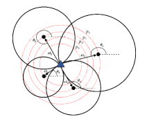
Figure 1: Measurement geometry of the hybrid localization model. The blue triangle represents the target and the black circles are the sensors. $p_{1}$, $p_{2}$, $p_{3}$ and $p_{4}$ represent the RSS measurements, $\theta_{1}$, $\theta_{2}$, $\theta_{3}$ and $\theta_{4}$ represent the AOA measurements, and $ct_{1}$, $ct_{2}$, $ct_{3}$ and $ct_{4}$ are the measurements corresponding to TOA.

The RSS measurement (average power $p_{i}$ (in dB)) received at the $i^{\text{th}}$ sensor is given as follows [45]:

$$p_{i}=p_{0}-10\alpha\ln\left(d_{i}\right)+\nu_{i},\;\forall i=1,\dots,m,$$ (4)

where $p_{0}$ is the signal power at the target and $\alpha$ is the path loss constant which depends on the medium. It is assumed that the parameters $p_{0}$ and $\alpha$ are known (determined using calibration [45]). The noise ($\nu_{i}$) in the measurements is assumed to be Gaussian noise. Integrating the RSS measurements from $m$ sensors we get:

$$\mathbf{p}=\eta\,\mathbf{g}_{\mathrm{RSS}}(\mathbf{r})+\mathbf{\boldsymbol{\xi}}_{\text{RSS}},$$ (5)

where $\mathbf{p}=[p_{1}-p_{0},\dots,p_{m}-p_{0}]^{T}$, $\eta=\frac{-10\alpha}{\mathrm{ln}(10)}$, $\mathbf{g}_{\mathrm{RSS}}(\mathbf{r})=[\ln(d_{1}),\dots,\ln(d_{m})]^{T}$ and $\mathbf{\boldsymbol{\xi}}_{\text{RSS}}=[\nu_{1},\dots,\nu_{m}]^{T}\sim\mathcal{N}(\boldsymbol{0},\boldsymbol{\Sigma}_{\text{RSS}})$.

The AOA measurement at the $i^{\text{th}}$ sensor is given by:

$$\theta_{i}=\tan^{-1}\left(\frac{r_{y}-s_{yi}}{r_{x}-s_{xi}}\right)+\omega_{i},\;\forall i=1,\dots,m,$$ (6)

where $\tan^{-1}\left(\cdot\right)$ is the 4-quadrant arctangent. If we assume the measurements are corrupted by Gaussian noise ($\omega_{i}$), then the AOA measurement model for $m$ sensors is given as:

$$\mathbf{\boldsymbol{\mathbf{\theta}}}=\mathbf{g}_{\mathrm{AOA}}(\mathbf{r})+\mathbf{\boldsymbol{\xi}}_{\text{AOA}},$$ (7)

where $\boldsymbol{\mathbf{\theta}}=[\theta_{1},\dots,\theta_{m}]^{T}$, $\mathbf{g}_{\mathrm{AOA}}(\mathbf{r})=[\tan^{-1}\left(\frac{r_{y}-s_{y1}}{r_{x}-s_{x1}}\right),\dots,\tan^{-1}\left(\frac{r_{y}-s_{ym}}{r_{x}-s_{xm}}\right)]^{T}$ and $\boldsymbol{\mathbf{\xi}}_{\text{AOA}}=[\omega_{1},\dots,\omega_{m}]^{T}\sim\mathcal{N}(\boldsymbol{0},\boldsymbol{\Sigma}_{\text{AOA}})$.

With the individual data models in (3), (5) and (7), the hybrid TOA-RSS-AOA measurement model can be obtained by stacking the individual models as given below:

$$\mathbf{q}=\begin{bmatrix}\mathbf{z}\\ \mathbf{p}\\ \mathbf{\boldsymbol{\theta}}\end{bmatrix}=\begin{bmatrix}\mathbf{\mathbf{\mathbf{g}}_{\text{TOA}}(\mathbf{r})}\\ \eta\,\mathbf{\mathbf{g}}_{\text{RSS}}(\mathbf{r})\\ \mathbf{\mathbf{g}}_{\text{AOA}}(\mathbf{r})\end{bmatrix}+\begin{bmatrix}\mathbf{\mathbf{\boldsymbol{\xi}}_{\text{TOA}}}\\ \mathbf{\boldsymbol{\xi}}_{\text{RSS}}\\ \mathbf{\boldsymbol{\xi}}_{\text{AOA}}\end{bmatrix}.$$ (8)

The FIM matrix for the hybrid model is defined as:

$$\mathbf{F}_{\mathrm{Hybrid}}=\mathbb{E}\left(\left(\frac{\partial\ln p(\mathbf{q};\mathbf{r})}{\partial\mathbf{r}}\right)\left(\frac{\partial\ln p(\mathbf{q};\mathbf{r})}{\partial\mathbf{r}}\right)^{T}\right)\in\mathbb{R}^{n\times n},$$ (9)

where $p(\mathbf{q};\mathbf{r})$ is the joint probability density function of the hybrid model. If we assume the noise in the three localization models ($\mathbf{\boldsymbol{\xi}}_{\text{TOA}}$, $\mathbf{\boldsymbol{\xi}}_{\text{RSS}}$ and $\mathbf{\boldsymbol{\xi}}_{\text{AOA}}$) are independent of each other, the joint probability density function will be proportional to the product of their individual probability density functions:

$$p\left(\mathbf{q};\mathbf{r}\right)\propto p\left(\mathbf{z};\mathbf{r}\right)\times p\left(\mathbf{p};\mathbf{r}\right)\times p\left(\mathbf{\boldsymbol{\theta}};\mathbf{r}\right).$$ (10)

The FIM for the hybrid measurements can therefore be written as [36]:

$$\mathbf{F}_{\mathrm{Hybrid}}(\mathbf{r})=\mathbf{F}_{\text{TOA}}(\mathbf{r})+\mathbf{F}_{\text{RSS}}(\mathbf{r})+\mathbf{F}_{\text{AOA}}(\mathbf{r}),$$ (11)

where $\mathbf{F}_{\text{TOA}}$, $\mathbf{F}_{\text{RSS}}$ and $\mathbf{F}_{\text{AOA}}$ are the individual FIM matrices and are given by (9) with the joint probability density function replaced by their individual probability density functions.

We first derive the CRLB matrix for TOA measurement. The probability density function of the observation vector $\mathbf{z}$ for the TOA model is given as:

$$\begin{split}p(\mathbf{z};\mathbf{r})=&\frac{\exp\left(-\frac{1}{2}(\mathbf{z}-\mathbf{g}_{\mathrm{TOA}}(\mathbf{r}))^{T}\boldsymbol{\Sigma}_{\text{TOA}}^{-1}(\mathbf{z}-\mathbf{g}_{\mathrm{TOA}}(\mathbf{r}))\right)}{(2\pi)^{\frac{m}{2}}\sqrt{\det(\boldsymbol{\Sigma}_{\text{TOA}})}}.\end{split}$$ (12)

Let $\hat{\mathbf{r}}$ be an unbiased estimator of the true target position, then the covariance matrix satisfies the following well-known inequality [46]:

$$\mathbb{E}\left[(\hat{\mathbf{r}}-\mathbf{r})(\hat{\mathbf{r}}-\mathbf{r})^{T}\right]\succeq\mathbf{C}_{\text{TOA}}(\mathbf{r})=\mathbf{F}_{\text{TOA}}^{-1}(\mathbf{r}),$$ (13)

where $\mathbf{C}_{\text{TOA}}(\mathbf{r})$ is the CRLB matrix and is given as:

$$\textrm{{C}}_{\text{TOA}}(\mathbf{r})=\textrm{{F}}_{\text{TOA}}^{-1}(\mathbf{r})=(\mathbf{J}^{T}\boldsymbol{\mathbf{\Sigma}}_{\text{TOA}}^{-1}\mathbf{J})^{-1},$$ (14)

where

$$\textbf{J}=\begin{bmatrix}\cos\theta_{1}&\sin\theta_{1}\\ \vdots&\vdots\\ \cos\theta_{m}&\sin\theta_{m}\end{bmatrix}=\begin{bmatrix}\frac{(\mathbf{r}-\mathbf{s}_{1})^{T}}{\|\mathbf{r}-\mathbf{s}_{1}\|}\\ \vdots\\ \frac{(\mathbf{r}-\mathbf{s}_{m})^{T}}{\|\mathbf{r}-\mathbf{s}_{m}\|}\end{bmatrix}.$$ (15)

The matrix J is referred to as the orientation matrix and each row of this matrix denotes the unit vector pointing in the direction of the line connecting the $i^{\mathrm{th}}$ sensor and the target.

From hereon, we will express the CRLB (or the FIM) matrix only in terms of $\mathbf{J}$ (as $\mathbf{C}_{\mathrm{TOA}}\left(\mathbf{J}\right)$) as it can be seen from (15) that the rows of $\mathbf{J}$ are only dependent on the orientation and not the actual position of the sensors or the target.

Remark 1.

The parameterization of orientation matrix J in (15) is stated in both the cartesian and polar forms. Most of the literature utilizes the polar form, which is specified in terms of ‘azimuth’ angle, thereby resulting in complex trigonometric expressions for the elements of the CRLB matrix. In order to simplify the design problem associated with the CRLB matrix, we will prefer the elements of the $\mathbf{J}$ to be in the cartesian coordinates. We can easily derive the respective azimuth angles from the cartesian representation, if required.

Similar to the derivation of $\textrm{{C}}_{\text{TOA}}$, the CRLB for RSS and AOA can be derived, and their FIM are given by [40]:

$$\mathbf{F}_{\text{RSS}}(\mathbf{J})=\eta^{2}\textbf{J}^{T}\textbf{D}\mathbf{\Sigma}_{\text{RSS}}^{-1}\textbf{D}\mathbf{J},$$ (16)

$$\mathbf{F}_{\text{AOA}}(\mathbf{J})=\mathbf{U}^{T}\textbf{J}^{T}\textbf{D}\mathbf{\Sigma}_{\text{AOA}}^{-1}\textbf{D}\mathbf{J}\mathbf{U},$$ (17)

where D is the distance matrix and U is the unitary matrix which are given by:

$$\begin{array}[]{ll}\textbf{D}=\mathrm{diag}\left(1/d_{1},\ldots 1/d_{m}\right)\mathrm{;\;}\textbf{U}=\begin{bmatrix}0&1\\ -1&0\end{bmatrix}.\end{array}$$ (18)

Remark 2.

The CRLB for RSS and AOA depends on the distance matrix D and the CRLB of the AOA model also involves an extra unitary matrix U (however, its elements are known). Before venturing into deriving the CRLB for the hybrid measurement model, it is important to note that any design objective which is based on the CRLB (for RSS and AOA) will depend on the target-sensor distances ($d_{i}$) (which is not known). So, a usual approach is to perform the optimal placement design based on an initial coarse target estimate. This initial target position (which maybe very rough) is assumed to be known by some alternate means and using which the orientation of the sensors are obtained. Although, this design of optimal placements by using a rough target location looks heuristic, it works very well in practice even if there is a slight mismatch between assumed target location in design and the true underlying unknown target location. In the numerical section, we will present MSE analysis for this mismatch issue.

With the individual FIMs mentioned in equations (14), (16) and (17), the FIM of the hybrid measurements ($\boldsymbol{\textrm{F}}_{\mathrm{Hybrid}}$) is given by:

$$\mathbf{F}_{\mathrm{Hybrid}}(\mathbf{J})= \mathbf{J}^{T}\boldsymbol{\mathbf{\Sigma}}_{\text{TOA}}^{-1}\mathbf{J}+\eta^{2}\textbf{J}^{T}\textbf{D}\mathbf{\Sigma}_{\text{RSS}}^{-1}\textbf{D}\mathbf{J}$$ (19)

$$+\mathbf{U}^{T}\textbf{J}^{T}\textbf{D}\mathbf{\Sigma}_{\text{AOA}}^{-1}\textbf{D}\mathbf{J}\mathbf{U}.$$

and the corresponding hybrid CRLB matrix is given as:

$$\textrm{{C}}_{\mathrm{Hybrid}}(\mathbf{J})= \left(\mathbf{J}^{T}\boldsymbol{\mathbf{\Sigma}}_{\text{TOA}}^{-1}\mathbf{J}+\eta^{2}\textbf{J}^{T}\textbf{D}\mathbf{\Sigma}_{\text{RSS}}^{-1}\textbf{D}\mathbf{J}\right.$$ (20)

$$\left.+\mathbf{U}^{T}\textbf{J}^{T}\textbf{D}\mathbf{\Sigma}_{\text{AOA}}^{-1}\textbf{D}\mathbf{J}\mathbf{U}\right)^{-1}$$

We would like to note that the hybrid CRLB matrix is the function of the orientation matrix, and we can optimize a scalar metric of CRLB to come up with optimal orientation matrix. We first consider the A-optimal criterion, where the objective is to minimize the trace of the CRLB matrix which results in the following optimization problem:

$$\min\limits_{\textbf{J}} \;\textrm{Tr}\Biggl{(}\biggl{(}\textbf{J}^{T}\mathbf{\Sigma}_{\text{TOA}}^{-1}\textbf{J}+\textbf{J}^{T}\eta^{2}\textbf{D}\mathbf{\Sigma}_{\text{RSS}}^{-1}\textbf{D}\textbf{J}$$ (21)

$$\left.\left.\,\,\,\,\,\,\,\,\,\,\,\,\,\,\,\,\,\,\,\,\,\,+\textbf{U}^{T}\textbf{J}^{T}\textbf{D}\mathbf{\Sigma}_{\text{AOA}}^{-1}\textbf{D}\textbf{J}\textbf{U}\right)^{-1}\right)$$

s.t. $$\;\mathbf{j}_{i}^{T}\mathbf{j}_{i}=1,i=1,\cdots,m,$$

where $\mathbf{j}_{i}$ is the $i^{\mathrm{th}}$ column of $\mathbf{J}^{T}$. Problem (21) can be rewritten as:

$$\min\limits_{\textbf{J}\in\mathcal{D}} \;\textrm{Tr}\Biggl{(}\biggl{(}\textbf{J}^{T}\left(\mathbf{\Sigma}_{\text{TOA}}^{-1}+\eta^{2}\textbf{D}\mathbf{\Sigma}_{\text{RSS}}^{-1}\textbf{D}\right)\textbf{J}$$ (22)

$$\left.\left.\,\,\,\,\,\,\,\,\,\,\,\,\,\,\,\,\,\,\,\,\,\,+\textbf{U}^{T}\textbf{J}^{T}\textbf{D}\mathbf{\Sigma}_{\text{AOA}}^{-1}\textbf{D}\textbf{J}\textbf{U}\right)^{-1}\right),$$

where the set $\mathcal{D}$ denotes the constraint $\textbf{j}_{i}^{T}\textbf{j}_{i}=1~{}\forall~{}i$. Using $\textbf{H}=\left[\textbf{J}^{T},\textbf{U}^{T}\textbf{J}^{T}\right]^{T}$ and $\textbf{R}=\text{\text{blkdiag}}\left(\mathbf{R}_{1},\mathbf{R}_{2}\right)$, where $\mathbf{R}_{1}=\mathbf{\Sigma}_{\text{TOA}}^{-1}+\eta^{2}\textbf{D}\mathbf{\Sigma}_{\text{RSS}}^{-1}\textbf{D}$ and $\mathbf{R}_{2}=\textbf{D}\mathbf{\Sigma}_{\text{AOA}}^{-1}\textbf{D}$, (22) can be compactly written as the following minimization problem:

$$\begin{array}[]{ll}\min\limits_{\textbf{H},\mathbf{J}\in\mathcal{D}}\textrm{Tr}((\textbf{H}^{T}\textbf{R}\textbf{H}){}^{-1})&\;\textrm{s.t. }\mathbf{H}=\begin{bmatrix}\mathbf{J}\\ \mathbf{J}\mathbf{U}\end{bmatrix}.\end{array}$$ (23)

The optimization problem (23) has a non-convex objective function and a non-convex constraint set. Moreover, the presence of inverse of the quadratic term inside $\mathrm{Tr}\left(\cdot\right)$ makes (23) a challenging optimization problem to solve. In the next section, we will propose an MM based algorithm to solve this non-linear optimization problem.

III PROPOSED MM BASED ALGORITHM

In this section, we first briefly discuss the MM technique, then give a detailed explanation of the proposed algorithm for the A optimal design, and later discuss the computational complexity and the convergence of the proposed algorithm. Finally, we present the extension of the proposed algorithm for D and E optimal design.

III-A MM technique

Majorization-minimization (MM) technique is used to develop problem-driven algorithms by exploiting the problem structure, and it works in two steps: a majorization step and a minimization step. In the majorization step, a surrogate function $g\left(\mathbf{x}|\mathbf{x}_{t}\right)$ that globally upperbounds the objective function $f\left(\mathbf{x}\right)$ (that is to be minimized) at a point $\mathbf{x}_{t}$ and satisfies the following properties is constructed:

$$g\left(\mathbf{x}|\mathbf{x}_{t}\right)\geq f\left(\mathbf{x}\right)\;\mathrm{and}\; g\left(\mathbf{x}_{t}|\mathbf{x}_{t}\right)=f\left(\mathbf{x}_{t}\right).$$ (24)

In the minimization step, the surrogate function is minimized to give the next update:

$$\mathbf{x}_{t+1}=\mathrm{arg}\;\underset{\mathbf{x}}{\mathrm{min}}\;g\left(\mathbf{x}|\mathbf{x}_{t}\right)$$ (25)

This leads to an iterative algorithm which is repeated until convergence to generate a non-increasing sequence $\left\{f\left(\mathbf{x}_{t}\right)\right\}_{t\in\mathbb{N}}$, since

$$f\left(\mathbf{x}_{t+1}\right)\leq g\left(\mathbf{x}_{t+1}|\mathbf{x}_{t}\right)\leq g\left(\mathbf{x}_{t}|\mathbf{x}_{t}\right)=f\left(\mathbf{x}_{t}\right).$$ (26)

The idea of MM can also be extended to maximization problems by replacing the upperbound minimization step to lowerbound maximization step. For more details on MM, its applications, and the construction of surrogate functions, please refer to [47] and the references therein. We would like to point out here that the general description on the MM technique included above is for problems having only primal variable. However, when we develop our algorithm later, we will show how the idea of MM can be extended to handle saddle point problems, which requires constructing MM upperbounds on both primal and dual variables.

III-B Proposed algorithm for A-optimal design problem

Let us restate the optimization problem for hybrid TOA-RSS-AOA:

$$\begin{array}[]{ll}\min\limits_{\textbf{H},\textbf{J}\in\mathcal{D}}\;\textrm{Tr}((\textbf{H}^{T}\textbf{R}\textbf{H})^{-1})&\;\textrm{s.t. }\textbf{H}=\begin{bmatrix}\textbf{J}\\ \textbf{J}\textbf{U}\end{bmatrix}.\end{array}$$ (27)

To deal with the complicated objective function in (27), we introduce an auxiliary variable $\mathbf{\Phi}$ and reformulate the original problem (27) using the Fenchel conjugate representation [48] of the objective function into the following equivalent saddle-point problem:

$$\begin{array}[]{ll}\max\limits_{\textbf{H},\textbf{J}\in\mathcal{D}}~{}\min\limits_{\mathbf{\Phi}\succeq 0}~{}\textrm{Tr}[\mathbf{\Phi}\textbf{H}^{T}\textbf{R}\textbf{H}]-\textrm{Tr}(\sqrt{\mathbf{\Phi}})&\;\textrm{s.t. }\textbf{H}=\begin{bmatrix}\textbf{J}\\ \textbf{J}\textbf{U}\end{bmatrix}.\end{array}$$ (28)

Here, the variables H and J can be interpreted as the primal variables, and the variable $\mathbf{\Phi}$ as the dual variable of the optimization problem. The equivalence of (27) and (28) is stated in the following Lemma.

Lemma 3.

The saddle-point problem (28) is equivalent to the original optimization problem (27).

Proof:

The proof of the Lemma can be found in the Appendix. ∎

We now proceed to derive an algorithm to solve the maximin problem in (28). Let

$$f\left(\textbf{H}\right)=\min\limits_{\mathbf{\Phi}\succeq 0}~{}\textrm{Tr}[\mathbf{\Phi}\textbf{H}^{T}\textbf{R}\textbf{H}]-\textrm{Tr}(\sqrt{\mathbf{\Phi}})$$ (29)

be a function only in the primal variable $\mathbf{H}$ and the optimization problem in (28) be compactly written as:

$$\begin{array}[]{ll}\max\limits_{\textbf{H},\textbf{J}\in\mathcal{D}}~{}f\left(\textbf{H}\right)&\;\textrm{s.t. }\textbf{H}=\begin{bmatrix}\textbf{J}\\ \textbf{J}\textbf{U}\end{bmatrix}.\\ \\ \end{array}$$ (30)

For a fixed $\mathbf{\Phi}$ and $\textbf{R}\in\mathbf{S}_{+}^{m}$, the term $\textrm{Tr}[\mathbf{\Phi}\textbf{H}^{T}\textbf{R}\textbf{H}]$ in (29) is a convex function in H. Since (30) is a maximization problem over $\mathbf{H}$, the MM technique can be utilized to lowerbound $f\left(\textbf{H}\right)$ (at a given $\mathbf{H}_{t}$, which of course can be obtained using a given $\mathbf{J}_{t}$) and iteratively maximize the lowerbound. We obtain the lowerbound via the following Lemma.

Lemma 4.

Given $\mathbf{H}_{t}$, the convex function $\mathrm{Tr}\left[\boldsymbol{\Phi}\mathbf{H}^{T}\mathbf{R}\mathbf{H}\right]$ can be lowerbounded as:

$$\mathrm{Tr}\left[\boldsymbol{\Phi}\mathbf{H}^{T}\mathbf{R}\mathbf{H}\right]\geq 2\mathrm{Tr}\left[\boldsymbol{\Phi}\mathbf{H}_{t}^{T}\mathbf{R}\mathbf{H}\right]-\mathrm{Tr}\left[\boldsymbol{\Phi}\mathbf{H}_{t}^{T}\mathbf{R}\mathbf{H}_{t}\right]$$ (31)

with equality achieved at $\mathbf{H}=\mathbf{H}_{t}$.

Proof:

The proof is based on the details in Section III-A of [47]. ∎

Using (31), $f\left(\textbf{H}\right)$ can be lowerbounded as:

$$f\left(\textbf{H}\right) \geq\min\limits_{\mathbf{\Phi}\succeq 0}\;2\textrm{Tr}[\mathbf{\Phi}\textbf{H}_{t}^{T}\textbf{R}\textbf{H}]-\textrm{Tr}[\mathbf{\Phi}\textbf{H}_{t}^{T}\textbf{R}\textbf{H}_{t}]-\textrm{Tr}(\sqrt{\mathbf{\Phi}})$$ (32)

$$\,\,\,\,\,\,\,\,\,\,\,\,\,\,\,\,\,\,\,\,\,\,\,\,\,\,\,\,\,\,\,\,\,\,\,\,\,\,\,\,\,\,\,\,\,\,\,\,\,\,\,\,\,\,\>\,\,\,\,\,\,\,\,\,\,\,\,\,\,\,\,\,\,\,\,\,\,\,\,\,\,\,\,\,\,\,\,\,\,\triangleq g_{f}\left(\mathbf{H}|\textbf{$\mathbf{H}$}_{t}\right)$$

giving rise to the following surrogate maximization problem:

$$\underset{\mathbf{H},\mathbf{J}\in\mathcal{D}}{\mathrm{max}} \;\underset{\mathbf{\Phi}\succeq 0}{\mathrm{min}}~{}2\textrm{Tr}[\mathbf{\Phi}\mathbf{H}_{t}^{T}\mathbf{R}\mathbf{H}]-\textrm{Tr}[\mathbf{\Phi}\textbf{$\mathbf{H}$}_{t}^{T}\mathbf{R}\mathbf{H}_{t}]-\textrm{Tr}(\sqrt{\mathbf{\Phi}})$$ (33)

$$\mathrm{s.t.\,\,\,\,\,} \;\mathbf{H}=\begin{bmatrix}\mathbf{J}\\ \mathbf{J}\mathbf{U}\end{bmatrix}$$

On substituting for R and H in (33), we get the following optimization problem:

$$\underset{\mathbf{J}\in\mathcal{D}}{\mathrm{max}}\;\underset{\mathbf{\Phi}\succeq 0}{\mathrm{min}} 2\textrm{Tr}[\mathbf{\Phi}\mathbf{J}_{t}^{T}\mathbf{R}_{1}\mathbf{J}]+2\textrm{Tr}[\mathbf{\Phi}\mathbf{U}^{T}\mathrm{\mathbf{J}}_{t}^{T}\mathbf{R}_{2}\mathbf{J}\mathbf{U}]-\textrm{Tr}(\sqrt{\mathbf{\Phi}})$$ (34)

$$-\textrm{Tr}[\mathbf{\Phi}\mathbf{J}_{t}^{T}\mathbf{R}_{1}\mathbf{J}_{t}]-\textrm{Tr}[\mathbf{\Phi}\mathbf{U}^{T}\mathbf{J}_{t}^{T}\mathbf{R}_{2}\mathbf{J}_{t}\mathbf{U}].$$

The constraint set $\mathcal{D}$ for $\mathbf{J}$ can be relaxed to $\mathcal{D}_{r}$ (which is defined as $\left\{\mathbf{j}_{i}\right\}$’s satisfying $\textbf{j}_{i}^{T}\textbf{j}_{i}\leq 1~{}\forall~{}i$) as the objective in (34) is linear in $\mathbf{J}$, and the optimum over $\mathbf{J}$ will occur only on the boundary and hence the relaxation will always be tight. With this relaxation, we can now reformulate the maximin problem in (34) into a minimax problem using the following minimax theorem:

Theorem 5.

[49] Let $\mathcal{X}$ and $\mathcal{Y}$ be compact convex sets. If $f:\mathcal{X}\times\mathcal{Y}\rightarrow\mathbb{R}$ is a continuous function that is concave-convex, i.e., $f\left(\cdot,y\right):\mathcal{X\rightarrow\mathbb{R}}$ is concave for fixed $y$, and $f\left(y,\cdot\right):\mathcal{Y\rightarrow\mathbb{R}}$ is convex for fixed $x$, then we have

$$\underset{x\in\mathcal{X}}{\mathrm{max}}\;\underset{y\in\mathcal{Y}}{\mathrm{min}}\;f\left(x,y\right)=\underset{y\in\mathcal{Y}}{\mathrm{min}}\;\underset{x\in\mathcal{X}}{\mathrm{max}}\;f\left(x,y\right)$$ (35)

Since the constraint sets (after relaxation) are compact convex sets, and the objective function in (34) is continuous, and convex in $\mathbf{\Phi}$ for a fixed $\mathbf{J}$ (the term $-\textrm{Tr}(\sqrt{\mathbf{\Phi}})$ is a convex function in $\mathbf{\Phi}$ via the Lieb’s concavity theorem [50]) and linear in $\mathbf{J}$ for a fixed $\mathbf{\Phi}$, we can switch the max and min term using Theorem 5 to arrive at the following minimax problem:

$$\min\limits_{\mathbf{\Phi}\succeq 0}~{}\max\limits_{\textbf{J}\in\mathcal{D}_{r}}{} 2\textrm{Tr}[\mathbf{\Phi}\textbf{J}_{t}^{T}\textbf{R}_{1}\textbf{J}]+2\textrm{Tr}[\mathbf{\Phi}\textbf{U}^{T}\textbf{J}_{t}^{T}\textbf{R}_{2}\textbf{J}\textbf{U}]-\textrm{Tr}(\sqrt{\mathbf{\Phi}})$$ (36)

$$-\textrm{Tr}[\mathbf{\Phi}\textbf{J}_{t}^{T}\textbf{R}_{1}\textbf{J}_{t}]-\textrm{Tr}[\mathbf{\Phi}\textbf{U}^{T}\textbf{J}_{t}^{T}\textbf{R}_{2}\textbf{J}_{t}\textbf{U}]$$

The minimax problem (36) has an inner maximization problem in $\mathbf{J}$ and an outer minimization problem in $\mathbf{\Phi}$. We will first solve the inner maximization problem in (36). Using $\textbf{Q}\triangleq\textbf{U}\mathbf{\Phi}\textbf{U}^{T}$, the inner maximization problem be written as:

$$\begin{array}[]{ll}\max\limits_{\textbf{J}\in D_{r}}\;2\textrm{Tr}[\textbf{J}_{t}^{T}\textbf{R}_{1}\textbf{J}\mathbf{\Phi}]+2\textrm{Tr}[\textbf{J}_{t}^{T}\textbf{R}_{2}\textbf{J}\textbf{Q}],\end{array}$$ (37)

Let

$$\mathbf{Z}=\mathbf{\Phi}\tilde{\mathbf{A}}_{1}+\textbf{Q}\tilde{\mathbf{A}}_{2},$$ (38)

with $\tilde{\mathbf{A}}_{1}\triangleq\textbf{J}_{t}^{T}\textbf{R}_{1}$ and $\tilde{\mathbf{A}}_{2}\triangleq\textbf{J}_{t}^{T}\textbf{R}_{2}$, then the optimization problem in (37) can be rewritten as:

$$\max\limits_{\textbf{J}\in D_{r}}\;2\sum_{i=1}^{m}\mathbf{j}_{i}^{T}\mathbf{z}_{i},$$ (39)

where $\mathbf{z}_{i}$ denotes the $i^{\mathrm{th}}$ column $\mathbf{Z}$. Problem (39) has the following closed-form solution:

$$\textbf{j}_{i}^{*}=\frac{\mathbf{z}_{i}}{\|\mathbf{z}_{i}\|}$$ (40)

Please note that the optimum occurs on the boundary of the constraint set $\mathcal{D}_{r}$ as noted before.

Eliminating the variable $\mathbf{J}$ from (36) by substituting for the optimal minimizer over $\mathbf{J}$ (i.e., $\textbf{j}_{i}^{*}=\frac{\mathbf{z}_{i}}{\|\mathbf{z}_{i}\|}$) gives the following minimization problem in the dual variable $\mathbf{\Phi}$:

$$\begin{array}[]{ll}\min\limits_{\mathbf{\Phi}\succeq 0}&2\stackrel{{\scriptstyle[}}{{i}}=1]{m}{\sum}||\mathbf{z}_{i}||-\textrm{Tr}[\mathbf{\Phi}\textbf{J}_{t}^{T}\textbf{R}_{1}\textbf{J}_{t}]-\textrm{Tr}[\mathbf{\Phi}\textbf{U}^{T}\textbf{J}_{t}^{T}\textbf{R}_{2}\textbf{J}_{t}\textbf{U}]\\ &-\textrm{Tr}(\sqrt{\mathbf{\Phi}}).\end{array}$$ (41)

Substituting for $\mathbf{z}_{i}$ from (38) in (41), we get:

$$\begin{array}[]{ll}\min\limits_{\mathbf{\Phi}\succeq 0}&2\stackrel{{\scriptstyle[}}{{i}}=1]{m}{\sum}\|\mathbf{\Phi}\mathbf{\tilde{\mathbf{a}}}_{i}^{1}+\textbf{Q}\tilde{\mathbf{a}}_{i}^{2}\|-\textrm{Tr}[\textbf{J}_{t}^{T}\textbf{R}_{1}\textbf{J}_{t}\mathbf{\Phi}]\\ &-\textrm{Tr}[\textbf{U}^{T}\textbf{J}_{t}^{T}\textbf{R}_{2}\textbf{J}_{t}\textbf{U}\mathbf{\Phi}]-\textrm{Tr}(\sqrt{\mathbf{\Phi}}),\end{array}$$ (42)

where $\tilde{\mathbf{a}}_{i}^{1}$ and $\tilde{\mathbf{a}}_{i}^{2}$ denote the $i^{\mathrm{th}}$ column of $\tilde{\mathbf{A}}_{1}$ and $\tilde{\mathbf{A}}_{2}$, respectively. Problem in (42) can be rewritten as:

$$\begin{array}[]{ll}\min\limits_{\mathbf{\Phi}\succeq 0}&2\stackrel{{\scriptstyle[}}{{i}}=1]{m}{\sum}\left\|\begin{bmatrix}\mathbf{\Phi},\textbf{Q}\end{bmatrix}\begin{bmatrix}\tilde{\mathbf{a}}_{i}^{1}\\ \tilde{\mathbf{a}}_{i}^{2}\end{bmatrix}\right\|-\textrm{Tr}[\textbf{J}_{t}^{T}\textbf{R}_{1}\textbf{J}_{t}\mathbf{\Phi}]\\ &-\textrm{Tr}[\textbf{U}^{T}\textbf{J}_{t}^{T}\textbf{R}_{2}\textbf{J}_{t}\textbf{U}\mathbf{\Phi}]-\textrm{Tr}(\sqrt{\mathbf{\Phi}}).\end{array}$$ (43)

Using $\tilde{\textbf{$\mathbf{\Phi}$}}=\begin{bmatrix}\mathbf{\Phi},\textbf{Q}\end{bmatrix}$ and $\mathbf{a}_{i}=\begin{bmatrix}\tilde{\mathbf{a}}_{i}^{1}\\ \tilde{\mathbf{a}}_{i}^{2}\end{bmatrix}$, the optimization problem (43) can be compactly written as:

$$\min\limits_{\mathbf{\Phi}\succeq 0}~{}2\stackrel{{\scriptstyle[}}{{i}}=1]{m}{\sum}\|\tilde{\textbf{$\mathbf{\Phi}$}}\mathbf{a}_{i}\|-\textrm{Tr}[\textbf{H}_{t}^{T}\textbf{R}\textbf{H}_{t}\mathbf{\Phi}]-\textrm{Tr}(\sqrt{\mathbf{\Phi}})\triangleq h\left(\mathbf{\Phi}\right).$$ (44)

The minimization problem (44) is a convex problem (semidefinite programming problem (SDP)) in $\mathbf{\Phi}$ and can be solved using some off-the-shelf interior point solvers. However, solving such SDP via the standard solvers will be computationally inefficient and will limit the application of our approach to only low dimensional problems. Therefore, we once again use “MM” to solve (44) which results in a double loop MM algorithm (by double loop we mean loop inside a loop). To this end, we construct a surrogate for the objective in (44) at some $\mathbf{\Phi}=\mathbf{\Phi}_{k}$. Since, (44) is a minimization problem, we first upperbound the term $\|\tilde{\textbf{$\mathbf{\Phi}$}}\mathbf{a}_{i}\|$ in $h\left(\mathbf{\Phi}\right)$ as per the following Lemma:

Lemma 6.

Given $\tilde{\mathbf{\Phi}}_{k}$, the $\ell_{2}$ norm function $\|\tilde{\textbf{$\mathbf{\Phi}$}}\mathbf{a}_{i}\|$ can be upperbounded as:

$$\|\tilde{\textbf{$\mathbf{\Phi}$}}\mathbf{a}_{i}\|\leq\frac{\|\tilde{\textbf{$\mathbf{\Phi}$}}\mathbf{a}_{i}\|^{2}}{2\|\tilde{\textbf{$\mathbf{\Phi}$}}_{k}\mathbf{a}_{i}\|}+\mathrm{const}.,$$ (45)

given that $||\tilde{\textbf{$\mathbf{\Phi}$}}_{k}\mathbf{a}_{i}||\neq 0$. Equality is achieved at $\mathbf{\Phi}=\mathbf{\Phi}_{k}$.

Proof:

The proof can be established using the details in Section III-A of [47]. ∎

Using Lemma 6, we can upperbound $h\left(\mathbf{\Phi}\right)$ as:

$$\begin{array}[]{ll}h\left(\mathbf{\Phi}\right)\leq&\stackrel{{\scriptstyle[}}{{i}}=1]{m}{\sum}\frac{\|\tilde{\textbf{$\mathbf{\Phi}$}}\mathbf{a}_{i}\|^{2}}{\|\tilde{\textbf{$\mathbf{\Phi}$}}_{k}\mathbf{a}_{i}\|}-\textrm{Tr}[\textbf{H}_{t}^{T}\textbf{R}\textbf{H}_{t}\mathbf{\Phi}]-\textrm{Tr}(\sqrt{\mathbf{\Phi}}),\end{array}$$ (46)

which can also be written as:

$$h\left(\mathbf{\Phi}\right)\leq \stackrel{{\scriptstyle[}}{{i}}=1]{m}{\sum}\frac{\mathbf{a}_{i}^{T}\tilde{\textbf{$\mathbf{\Phi}$}}^{T}\tilde{\textbf{$\mathbf{\Phi}$}}\mathbf{a}_{i}}{\|\tilde{\textbf{$\mathbf{\Phi}$}}_{k}\mathbf{a}_{i}\|}-\textrm{Tr}[\textbf{H}_{t}^{T}\textbf{R}\textbf{H}_{t}\mathbf{\Phi}]-\textrm{Tr}(\sqrt{\mathbf{\Phi}}).$$ (47)

Using $\mathbf{A}=\stackrel{{\scriptstyle[}}{{i}}=1]{m}{\sum}\frac{\mathbf{a}_{i}\mathbf{a}_{i}^{T}}{\|\tilde{\textbf{$\mathbf{\Phi}$}}_{k}\mathbf{a}_{i}\|}$, (47) can be rewritten as:

$$\begin{array}[]{ll}h\left(\mathbf{\Phi}\right)\leq&\textrm{Tr}(\tilde{\mathbf{\Phi}}\mathbf{A}\tilde{\mathbf{\Phi}}^{T})-\textrm{Tr}[\mathbf{\Phi}\textbf{H}_{t}^{T}\textbf{R}\textbf{H}_{t}]-\textrm{Tr}(\sqrt{\mathbf{\Phi}})\\ &\,\,\,\,\,\,\,\,\,\,\,\,\,\,\,\,\,\,\,\,\,\,\,\,\,\,\,\,\,\,\,\,\,\,\,\,\,\,\,\,\,\,\>\,\,\,\,\,\,\,\,\,\,\,\,\,\,\,\,\,\,\,\,\,\,\,\,\,\,\,\,\,\,\,\,\,\,\,\triangleq\tilde{g}_{h}\left(\mathbf{\Phi}|\mathbf{\Phi}_{k}\right)\end{array}$$ (48)

and the associated surrogate minimization problem can be written as:

$$\min\limits_{\mathbf{\Phi}\succeq 0}~{}\tilde{g}_{h}\left(\mathbf{\Phi}|\mathbf{\Phi}_{k}\right).$$ (49)

Problem (49) does not have a closed-form solution and therefore, we once again upperbound $\tilde{g}_{h}\left(\mathbf{\Phi}|\mathbf{\Phi}_{k}\right)$ at $\mathbf{\Phi}=\mathbf{\Phi}_{k}$. Let $\lambda_{1}=\lambda_{\mathrm{max}}\left(\mathbf{A}\right)$ and $\tilde{\mathbf{A}}=\mathbf{A}-\lambda_{1}\mathbf{I}$, then (49) can be rewritten as:

$$\min\limits_{\mathbf{\Phi}\succeq 0}~{}\textrm{Tr}(\tilde{\mathbf{\Phi}}\tilde{\mathbf{A}}\tilde{\mathbf{\Phi}}^{T})+\lambda_{1}\textrm{Tr}\left(\tilde{\mathbf{\Phi}}^{T}\tilde{\mathbf{\Phi}}\right)-\textrm{Tr}[\textbf{H}_{t}^{T}\textbf{R}\textbf{H}_{t}\mathbf{\Phi}]-\textrm{Tr}(\sqrt{\mathbf{\Phi}}).$$ (50)

The first term $\textrm{Tr}(\tilde{\mathbf{\Phi}}\tilde{\mathbf{A}}\tilde{\mathbf{\Phi}}^{T})$ is a concave function in $\tilde{\mathbf{\Phi}}$ and can be linearized using the first order Taylor series expansion as:

$$\textrm{Tr}(\tilde{\mathbf{\Phi}}\tilde{\mathbf{A}}\tilde{\mathbf{\Phi}}^{T})\leq-\textrm{Tr}(\tilde{\mathbf{\Phi}}_{k}\tilde{\mathbf{A}}\tilde{\mathbf{\Phi}}_{k}^{T})+2\textrm{Tr}(\tilde{\mathbf{\Phi}}_{k}\tilde{\mathbf{A}}\tilde{\mathbf{\Phi}}^{T})$$ (51)

Using (51), $\tilde{g}_{h}\left(\mathbf{\Phi}|\mathbf{\Phi}_{k}\right)$ can be upperbounded as:

$$\tilde{g}_{h}\left(\mathbf{\Phi}|\mathbf{\Phi}_{k}\right)\leq -\textrm{Tr}(\tilde{\mathbf{\Phi}}_{k}\tilde{\mathbf{A}}\tilde{\mathbf{\Phi}}_{k}^{T})+2\textrm{Tr}(\tilde{\mathbf{\Phi}}_{k}\tilde{\mathbf{A}}\tilde{\mathbf{\Phi}}^{T})+\lambda_{1}\textrm{Tr}\left(\tilde{\mathbf{\Phi}}^{T}\tilde{\mathbf{\Phi}}\right)$$ (52)

$$-\textrm{Tr}[\textbf{H}_{t}^{T}\textbf{R}\textbf{H}_{t}\mathbf{\Phi}]-\textrm{Tr}(\sqrt{\mathbf{\Phi}})\triangleq g_{h}\left(\mathbf{\Phi}|\mathbf{\Phi}_{k}\right).$$

It is to be noted that $g_{h}\left(\mathbf{\Phi}|\mathbf{\Phi}_{k}\right)$ will also tightly upperbound $h\left(\mathbf{\Phi}\right)$ at $\mathbf{\Phi}=\mathbf{\Phi}_{k}$. Thus, we arrive at the following surrogate minimization problem:

$$\min\limits_{\mathbf{\Phi}\succeq 0} 2\textrm{Tr}(\tilde{\mathbf{\Phi}}_{k}\tilde{\mathbf{A}}\tilde{\mathbf{\Phi}}^{T})+\lambda_{1}\textrm{Tr}\left(\tilde{\mathbf{\Phi}}^{T}\tilde{\mathbf{\Phi}}\right)-\textrm{Tr}[\textbf{H}_{t}^{T}\textbf{R}\textbf{H}_{t}\mathbf{\Phi}]$$ (53)

$$-\textrm{Tr}(\sqrt{\mathbf{\Phi}}).$$

Substituting for $\tilde{\mathbf{\Phi}}$ in (53) and using $\mathbf{B}=\left[\mathbf{B}_{1}\boldsymbol{,}\mathbf{B}_{2}\right]=\tilde{\mathbf{\Phi}}_{k}\tilde{\mathbf{A}}$, we get the following optimization problem:

$$\begin{array}[]{ll}\min\limits_{\mathbf{\Phi}\succeq 0}&2\textrm{Tr}\left(\left[\mathbf{B}_{1}\boldsymbol{,}\mathbf{B}_{2}\right]\begin{bmatrix}\mathbf{\Phi}\\ \mathbf{Q}\end{bmatrix}\right)+2\lambda_{1}\textrm{Tr}\left(\mathbf{\Phi}^{2}\right)-\textrm{Tr}[\textbf{H}_{t}^{T}\textbf{R}\textbf{H}_{t}\mathbf{\Phi}]\\ &-\textrm{Tr}(\sqrt{\mathbf{\Phi}}).\end{array}$$ (54)

With $\lambda=2\lambda_{1}$ and substituting $\mathbf{Q}$ in (54), we get:

$$\min\limits_{\mathbf{\Phi}\succeq 0} \textrm{Tr}((\mathbf{B}_{1}+\mathbf{B}_{1}^{T})\mathbf{\Phi})+\textrm{Tr}(\mathbf{U}^{T}(\mathbf{B}_{2}+\mathbf{B}_{2}^{T})\mathbf{U}\mathbf{\mathbf{\Phi}})+\lambda\textrm{Tr}\left(\mathbf{\Phi}^{2}\right)$$ (55)

$$-\textrm{Tr}[\textbf{H}_{t}^{T}\textbf{R}\textbf{H}_{t}\mathbf{\Phi}]-\textrm{Tr}(\sqrt{\mathbf{\Phi}})$$

Using $\textbf{C}=\mathbf{B}_{1}+\mathbf{B}_{1}^{T}+\mathbf{U}^{T}(\mathbf{B}_{2}+\mathbf{B}_{2}^{T})\mathbf{U}-\textbf{H}_{t}^{T}\textbf{R}\textbf{H}_{t}$, (55) can be compactly written as:

$$\min\limits_{\mathbf{\Phi}\succeq 0}\;\textrm{Tr}(\textbf{C}\mathbf{\Phi})+\lambda\textrm{Tr}(\boldsymbol{\mathbf{\Phi}^{2}})-\textrm{Tr}(\sqrt{\mathbf{\Phi}})$$ (56)

The optimal solution of the above mentioned problem can be computed easily based on the eigenvalue decomposition of $\mathbf{C}$ and solving scalar cubic equations. Suppose $\mathbf{V}$ and $\mathbf{E}$ denote the matrices containing the eigenvectors and eigenvalues of $\mathbf{C}$, then the minimizer for the problem will be $\mathbf{V}\mathbf{X}\mathbf{V}^{T}$, where any diagonal element of the matrix $\mathbf{X}$ will be computed by solving the following scalar problems:

$$\begin{array}[]{ll}\min\limits_{X_{ii}>0}E_{ii}X_{ii}+\lambda X_{ii}^{2}-\sqrt{X_{ii}}&\;\forall i\end{array}$$ (57)

The KKT condition for the above problem will be:

$$\begin{array}[]{ll}E_{ii}+2\lambda X_{ii}^{*}-\frac{1}{2\sqrt{X_{ii}^{*}}}=0&\;\forall i\end{array}$$ (58)

Using $\tilde{X}_{ii}^{*}=\sqrt{X_{ii}^{*}}$, and then multiplying both sides of equation (58) with $2\tilde{X}_{ii}^{*}$ gives:

$$\begin{array}[]{ll}4\lambda\left(\tilde{X}{}_{ii}^{*}\right)^{3}+2E_{ii}\tilde{X}_{ii}^{*}-1=0&\;\forall i\end{array},$$ (59)

which is nothing but a cubic equation whose positive real root will give the optimum $\mathbf{X}^{*}$.

III-C Solving the D and E optimal design problems

The algorithm proposed in the previous subsection can be extended to D and E optimal criteria as follows.

In D-optimal design, the problem is to solve the following maximization problem:

$$\underset{\mathbf{H},\mathbf{J}\in\mathcal{D}}{\mathrm{max}} \;\mathrm{log}\left|\mathbf{H}^{T}\mathbf{R}\mathbf{H}\right|,\;\textrm{s.t. {H}}=\begin{bmatrix}\textbf{J}\\ \textbf{J}\textbf{U}\end{bmatrix}.$$ (60)

The presence of quadratic term inside $\mathrm{log}\left|\cdot\right|$ makes (60) a challenging problem to solve. Similar to the A-optimal case, we use the Fenchel conjugate representation of the log determinant function, which is given as:

$$\mathrm{log}\left|\mathbf{A}\right|=\underset{\mathbf{B}\succeq 0}{\mathrm{min}}\>\mathbf{Tr}\left(\mathbf{A}\mathbf{B}\right)-\mathrm{log}\left|\mathbf{B}\right|,$$ (61)

to reformulate problem (60) into the following equivalent saddle-point problem:

$$\max\limits_{\textbf{H},\mathbf{J}\in\mathcal{D}} \;\min\limits_{\mathbf{\Phi}\succeq 0}~{}\textrm{Tr}[\mathbf{\Phi}\textbf{H}^{T}\textbf{R}\textbf{H}]-\log|\mathbf{\Phi}|$$ (62)

s. t. $$\textbf{H}=\begin{bmatrix}\textbf{J}\\ \textbf{J}\textbf{U}\end{bmatrix}.$$

Similar to the proof of Lemma 3 in the A-optimal design, it can be shown that the maximin problem (62) is equivalent to the problem (60).

In the case of E-optimal design, the objective is to solve the following maximization problem:

$$\underset{\textbf{H},\mathbf{J}\in\mathcal{D}}{\mathrm{max}} \mathrm{\lambda}_{\mathrm{min}}\left(\mathbf{H}^{T}\mathbf{R}\mathbf{H}\right)\;\textrm{s.t. {H}}=\begin{bmatrix}\textbf{J}\\ \textbf{J}\textbf{U}\end{bmatrix}.$$ (63)

(Typically, in E optimal design, the objective is to minimize the maximum eigen value of the matrix $\left(\mathbf{H}^{T}\mathbf{R}\mathbf{H}\right)^{-1}$ which is equivalent to maximizing the minimum eigen value of the matrix $\left(\mathbf{H}^{T}\mathbf{R}\mathbf{H}\right)$). Unlike A and D optimal case, there is no such Fenchel representation readily available for the $\mathrm{\lambda}_{\mathrm{min}}\left(\cdot\right)$ function. So, we resort to the Lagrangian dual formulation to arrive at the saddle-point formulation. We first consider the epigraph reformulation of the problem in (63):

$$\underset{\mathbf{H},\mathbf{\mathbf{J}\in\mathcal{D}},\alpha}{\mathrm{max}} \;\alpha$$ (64)

s.t. $$\;\textbf{H}^{T}\textbf{R}\textbf{H}\succeq\alpha\mathbf{I},\;\textbf{H}=\begin{bmatrix}\textbf{J}\\ \textbf{J}\textbf{U}\end{bmatrix}.$$

The Lagrangian dual of the problem in (64) is given by:

$$\max\limits_{\textbf{H},\mathbf{J}\in\mathcal{D},\alpha}\>\min\limits_{\mathbf{\Phi}\succeq 0} ~{}\alpha+\textrm{Tr}[\mathbf{\Phi}\textbf{H}^{T}\textbf{R}\textbf{H}]-\alpha\textrm{Tr}[\mathbf{\Phi}]$$ (65)

s.t. $$\;\textbf{H}=\begin{bmatrix}\textbf{J}\\ \textbf{J}\textbf{U}\end{bmatrix},$$

where $\mathbf{\Phi}$ is the Lagrangian dual variable. On rearranging the terms in (65), we get:

$$\max\limits_{\textbf{H},\mathbf{J}\in\mathcal{D},\alpha}\>\min\limits_{\mathbf{\Phi}\succeq 0} ~{}\textrm{Tr}[\mathbf{\Phi}\textbf{H}^{T}\textbf{R}\textbf{H}]-\alpha\left(1-\textrm{Tr}[\mathbf{\Phi}]\right)$$ (66)

s.t. $$\;\textbf{H}=\begin{bmatrix}\textbf{J}\\ \textbf{J}\textbf{U}\end{bmatrix}.$$

Here we would like to note that in the saddle-point formulations in (28), (62) and (66), the term containing the primal variable ‘$\mathbf{H}$’ remains the same, and the difference is in the second term (which is a function only in the dual variable ‘$\mathbf{\Phi}$’). Thus, the difference between the algorithms for the different optimal criteria will only be in the update for ‘$\mathbf{\Phi}$’. Therefore, in the following we will discuss only necessary changes in the update of $\mathbf{\Phi}$ for D and E optimal design problems.

In D-optimal design, to update $\mathbf{\Phi}$, we construct surrogate using MM (at $\mathbf{\Phi}=\mathbf{\Phi}_{k}$) in a manner similar to the A-optimal design and get the following minimization problems:

$$\begin{array}[]{ll}\min\limits_{X_{ii}>0}E_{ii}X_{ii}+\lambda X_{ii}^{2}-\log(X_{ii})&\;\forall i\end{array}$$ (67)

The KKT condition for the above problem is:

$$\begin{array}[]{ll}E_{ii}+2\lambda X_{ii}^{*}-\frac{1}{X_{ii}^{*}}&=0\end{array}\;\forall i$$ (68)

which is a quadratic equation and the optimal solution will be its positive root:

$$X_{ii}^{*}=\frac{-E_{ii}+\sqrt{E_{ii}^{2}+8\lambda}}{4\lambda}\;\;\forall i$$ (69)

In E-optimal design case, following the same steps as in A-optimal design, we arrive at the following surrogate (minimax) problem:

$$\min\limits_{\mathbf{\Phi}\succeq 0}~{}\max\limits_{\textbf{J}\in\mathcal{D}_{r},\alpha} 2\textrm{Tr}[\textbf{J}_{t}^{T}\textbf{R}_{1}\textbf{J}\mathbf{\Phi}]-\textrm{Tr}[\textbf{J}_{t}^{T}\textbf{R}_{1}\textbf{J}_{t}\mathbf{\Phi}]+2\textrm{Tr}[\textbf{J}_{t}^{T}\textbf{R}_{2}\textbf{J}\mathbf{Q}]$$ (70)

$$-\textrm{Tr}[\textbf{J}_{t}^{T}\textbf{R}_{2}\textbf{J}_{t}\mathbf{Q}]+\alpha(1-\textrm{Tr}[\mathbf{\Phi}]).$$

Here, we first eliminate the variable $\alpha$ and get:

$$\min\limits_{\mathbf{\Phi}\succeq 0}~{}\max\limits_{\textbf{J}\in\mathcal{D}_{r}} \;2\textrm{Tr}[\textbf{J}_{t}^{T}\textbf{R}_{1}\textbf{J}\mathbf{\Phi}]-\textrm{Tr}[\textbf{J}_{t}^{T}\textbf{R}_{1}\textbf{J}_{t}\mathbf{\Phi}]+2\textrm{Tr}[\textbf{J}_{t}^{T}\textbf{R}_{2}\textbf{J}\mathbf{Q}]$$ (71)

$$\,\,\,\,\,\,\,\,\,\,\,\,\,\,\,\,\,\,\,\,\,\,\,\,\,\,\,\,\,\,\,\,\,\,\,\,\,\,\,\,\,\,\,\,\,\,\,\,\,\,\,\,\,\,\,\,\,\,\,\,\,\,\,\,\,\,\,\,\,\,\,\,\,\,-\textrm{Tr}[\textbf{J}_{t}^{T}\textbf{R}_{2}\textbf{J}_{t}\mathbf{Q}]$$

s.t. $$\;\textrm{Tr}[\mathbf{\Phi}]\geq 1.$$

The constraint in (71) will be tight as the objective in (71) is linear in $\mathbf{\Phi}$, and therefore, the optimum will occur at the boundary of the constraint set. Following the steps similar to the A-optimal design for eliminating $\mathbf{J}$, we arrive at the following optimization problem:

$$\min\limits_{\mathbf{\Phi}\succeq 0} \;2\sum_{i=1}^{m}\left\|\tilde{\textbf{$\mathbf{\Phi}$}}\mathbf{a}_{i}\right\|-\textrm{Tr}[\mathbf{\Phi}\textbf{H}_{t}^{T}\textbf{R}\textbf{H}_{t}]$$ (72)

s.t. $$\;\textrm{Tr}[\mathbf{\Phi}]=1,$$

Problem in (72) is a convex optimization problem (an SDP). Unlike the A and D optimal case, solving the problem in (72) via MM is very challenging, so we prefer to solve (72) via standard interior point methods like CVX. The pseudo-code of the proposed algorithm for TOA-RSS-AOA measurements is given in Algorithm 1, with Algorithm 2 and Algorithm 3 describing the $\mathbf{\Phi}$ update for the three optimal designs.

Algorithm 1 Pseudo-code of the proposed algorithm (A, D and E optimal design)

• $m$, $n$, $\mathbf{D}$, $\boldsymbol{\Sigma}_{\text{TOA}}$, $\boldsymbol{\Sigma}_{\text{RSS}}$, $\boldsymbol{\Sigma}_{\text{AOA}}$, $\boldsymbol{\mathbf{U}}$ and $\epsilon=10^{-3}$

  1. Initialize $\mathbf{J}_{0}$ and $\boldsymbol{\Phi}{}_{0}$

  2. Iterate: Given $\mathbf{J}_{t}$, do the $\left(t+1\right)^{\mathbf{th}}$ step.

     1. Compute $\mathbf{H}_{t}$, $\mathbf{\tilde{\mathbf{A}}_{1}}$ and $\tilde{\mathbf{A}}_{2}$.

     2. Update $\boldsymbol{\Phi}$ using Algorithm 2 (for A- and D- optimal design) and Algorithm 3 (for E-optimal design).

     3. Compute $\mathbf{Z}$.

     4. Solve (40) to obtain $\mathbf{J}_{t+1}$.

     5. If $\left\|\mathbf{J}_{t+1}-\mathbf{J}_{t}\right\|_{F}/\left\|\mathbf{J}_{t}\right\|_{F}<\epsilon$, stop and return $\mathbf{J}_{t+1}$.

• $\mathbf{J}^{*}$ is the value of $\mathbf{J}$ obtained at the convergence of the loop.

Algorithm 2 Pseudo code to update $\boldsymbol{\Phi}$ in A and D optimal design

• $\mathbf{H}_{t}$, $\tilde{\textbf{A}}_{1}$, $\tilde{\textbf{A}}_{2}$ and $\epsilon=10^{-3}$

1. Iterate: Given $\boldsymbol{\Phi}{}_{k}$, do the $\left(k+1\right)^{\mathbf{th}}$ step.

   1. Compute $\tilde{\boldsymbol{\Phi}}{}_{k}$, $\mathbf{A}$, $\lambda_{\mathrm{max}}\left(\mathbf{A}\right)$, $\mathbf{B}=\left[\mathbf{B}_{1},\mathbf{B}_{2}\right]$ and $\mathbf{C}$.

   2. Compute the EVD $\mathbf{C}=\mathbf{V}\mathbf{E}\mathbf{V}^{T}$.

   3. • A-optimal design

        Solve (59) to obtain $X_{ii}^{*}\;\forall i$.

      • D-optimal design

        Solve (69) to obtain $X_{ii}^{*}\;\forall i$.

   4. $\boldsymbol{\Phi}{}_{k+1}=\mathbf{V}\mathbf{X}^{*}\mathbf{V}^{T}$.

   5. If $\left\|\mathbf{\boldsymbol{\Phi}}_{k+1}-\mathbf{\boldsymbol{\Phi}}_{k}\right\|_{F}/\left\|\mathbf{\boldsymbol{\Phi}}_{k}\right\|_{F}<\epsilon$, stop and return $\mathbf{\boldsymbol{\Phi}}_{k+1}$.

• $\mathbf{\boldsymbol{\Phi}}^{*}$ is the value of $\mathbf{\boldsymbol{\Phi}}$ obtained at the convergence of the loop.

Algorithm 3 Pseudo code to update $\boldsymbol{\Phi}$ in E-optimal design

• $\mathbf{H}_{t}$

1. Solve the SDP in (72) using CVX to update $\mathbf{\boldsymbol{\Phi}}$.

• $\mathbf{\boldsymbol{\Phi}}^{*}$ is the optimal value obtained using CVX.

Remark 7.

The proposed method can be extended for the 3D case, however, the AOA measurement model for the 3D case cannot be handled in the current framework as the CRLB expressions in the case of AOA model for the 3D will have sum of two terms (corresponding to the azimuth and elevation angles) and reformulating the hybrid CRLB matrix into the form similar to the problem in (23) is not possible. Nonetheless, we can extend the proposed algorithm to the reduced hybrid model of TOA-RSS and in the following we shall discuss the same. The orientation matrix $\mathbf{J}$ in the 3D case is defined as follows:

$$\mathbf{J}=\begin{bmatrix}\cos\phi_{1}\cos\theta_{1}&\cos\phi_{1}\sin\theta_{1}&\sin\phi_{1}\\ \vdots&\vdots&\vdots\\ \cos\phi_{m}\cos\theta_{m}&\cos\phi_{m}\sin\theta_{1}&\sin\phi_{m}\end{bmatrix}$$ (73)

where $\phi$ is the elevation angle, and the A-optimal design problem is given by:

$$\begin{aligned} \underset{\mathbf{J}\in\mathcal{D}}{\mathrm{min}}\;&\mathrm{Tr}\left(\left(\mathbf{J}^{T}\mathbf{R}\mathbf{J}\right)^{-1}\right)\end{aligned},$$ (74)

where $\mathbf{R}=\mathbf{\Sigma}_{\text{TOA}}^{-1}+\eta^{2}\textbf{D}\mathbf{\Sigma}_{\text{RSS}}^{-1}\textbf{D}.$

The above mentioned problem formulation looks similar to (23) and the proposed method can be easily adapted to solve for a minimizer of (74).

III-D Computational complexity and proof of convergence

We first discuss the computational complexity of the proposed algorithm. The update of the primal variable for the three optimal designs requires the computation of the matrices $\mathbf{H}_{t}$, $\mathbf{\tilde{\mathbf{A}}}_{1}$, $\tilde{\mathbf{A}}_{2}$ and $\mathbf{Z}$ (which has a total complexity of $\mathcal{O}\left(m^{2}n+mn^{2}\right)$) in each iteration. The update of the dual variable in the A and D optimal designs require the computations of $\tilde{\boldsymbol{\Phi}}{}_{k}$, $\mathbf{A}$, $\lambda_{\mathrm{max}}\left(\mathbf{A}\right)$ and $\mathbf{B}$ (which has a total complexity of $\mathcal{O}\left(mn^{2}+n^{3}\right)$), $\mathbf{C}$ (which has a complexity of $\mathcal{O}\left(m^{2}n\right)$) and the EVD of $\mathbf{C}$ (which requires $\mathcal{O}\left(n^{3}\right)$ flops) in each inner loop iteration. As $m>n$, the overall complexity of the proposed algorithm for A and D optimal design is therefore of the order $\mathcal{O}\left(m^{2}n\right)$. For E-optimal design, the dual problem is an SDP and the dual variable $\boldsymbol{\Phi}$ is updated using interior point methods. According to [51], the average worst case computation complexity of semi-definite programming problem is of the order $\mathcal{O}\left(m^{4.5}\right)$. Table II summarizes the overall computation complexity of the proposed algorithm using the three different optimal designs.

TABLE II: COMPUTATION COMPLEXITY OF THE PROPOSED ALGORITHM FOR A, D AND E OPTIMAL DESIGNS

Optimality Criterion	A-optimal	D-optimal	E-optimal
Computation Complexity	$\mathcal{O}\left(m^{2}n\right)$	$\mathcal{O}\left(m^{2}n\right)$	$\mathcal{O}\left(m^{4.5}\right)$

We now briefly discuss the proof of convergence of the proposed algorithm. As the proposed algorithm is a double loop MM algorithm, we will prove the convergence of the MM updates over the primal variable $\mathbf{H}$ and the dual variable $\mathbf{\Phi}$ separately. Furthermore, since the convergence of the MM update over $\mathbf{H}$ depends on the convergence of the MM update over $\mathbf{\Phi}$, we will first state the following Lemma:

Lemma 8.

The iterative steps of the MM update over dual variable $\mathbf{\Phi}$ in the proposed algorithm converge to the global minimum of the dual problem (44).

Proof:

From (26) we know that the sequence $\left\{\mathbf{\Phi}_{k}\right\}$ generated by the MM update of dual variable $\mathbf{\Phi}$ will monotonically decrease the dual objective function $h\left(\mathbf{\Phi}\right)$. The convergence of the sequence $\left\{h\left(\mathbf{\Phi}_{k}\right)\right\}$ to a finite value at a stationary point of the dual problem can be proved using the details in Section II-C of [47] and the references therein. Moreover, since the dual problem is a convex problem, the stationary point will also be the global minimizer of $h\left(\mathbf{\Phi}\right)$. ∎

Now that the convergence of the MM update over dual variable is established in Lemma 8, we move on to state the convergence of the MM update over the primal variable.

Lemma 9.

The iterative steps of the MM update over primal variable $\mathbf{H}$ in the proposed algorithm converge to a KKT point of the primal problem (27).

Proof:

Since, the primal problem is a maximization problem, the sequences $\left\{\mathbf{H}_{t}\right\}$ generated by the MM update of primal variable $\mathbf{H}$ will monotonically increase the objective function $f\left(\mathbf{H}\right)$. Similar to the details mentioned in Lemma 8, the sequence $\left\{f\left(\mathbf{H}_{t}\right)\right\}$ generated can also be proved to converge to a finite value, and that will be a KKT point of the primal problem. ∎

IV NUMERICAL SIMULATIONS AND RESULTS

In this section, we discuss various numerical simulations under different noise settings and design parameters to evaluate the performance of the proposed method.

IV-A Convergence of the proposed algorithm

First, we check the convergence of the proposed algorithm and compare its performance with the naive way of placing sensors uniformly on a circle of chosen radius encompassing the target. Let us consider that there are 4 sensors which are to be optimally placed and the target is at the centre and the sensors are to be placed on the circle with radius equal to $10$ meters. For the uniform placement, let us take the following orientation:

$$\begin{array}[]{ll}\textbf{J}_{\text{uni}}^{T}=\begin{bmatrix}10&0&-10&0\\ 0&10&0&-10\end{bmatrix}.\end{array}$$ (75)

The noise covariance matrices corresponding to TOA, RSS and AOA are taken to be non-diagonal with its elements randomly sampled from uniform distribution $\mathcal{U}\left[0,1\right]$.

In Fig. 2, we show the objective (A, D and E design criteria, for D-optimal we plot $-\mathrm{log}\left|\left(\mathbf{H}^{T}\mathbf{R}\mathbf{H}\right)\right|$ and for E-optimal we plot $\lambda_{\mathrm{max}}\left(\left(\mathbf{H}^{T}\mathbf{R}\mathbf{H}\right)^{-1}\right)$) vs iterations. The primal variable ($\mathbf{J}$) in the proposed algorithm (for all three designs) is initialized with the uniform configuration in (75) and the variable $\boldsymbol{\Phi}$ (in the case of A and D-optimal design) is initialized randomly. It can be seen from the plots in Fig. 2 that the proposed algorithm monotonically decreases the design objective and eventually converges to an optimum. The optimal configurations obtained are also shown in Fig. 2.

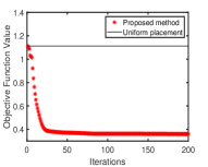
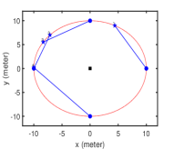
(a) A-optimal design

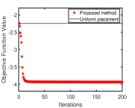
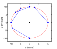
(b) D-optimal design

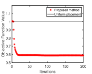
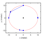
(c) E-optimal design

Figure 2: Convergence plot and corresponding sensor placement for 2D hybrid TOA-RSS-AOA under correlated noise. Top: convergence plots; Bottom: sensor placement with black square: target; blue circle: initial sensors’ positions; blue pentagram: final sensors’ positions.

The initialization using the uniform placement also gives a comparison (in terms of the design objective) between this uniform geometry and the optimal sensor geometry obtained using the proposed algorithm. The optimal sensor placement obtained via proposed algorithm using A, D and E optimal designs show an improvement of $40\%-70\%$ with respect to the uniform placement. This shows that improvement in localization accuracy can be achieved using sensor-target geometry obtained by the proposed algorithm.

IV-B Proposed algorithm for the 3D case

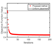
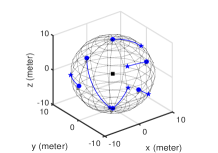
(a) A-optimal design

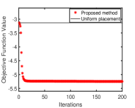
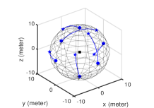
(b) D-optimal design

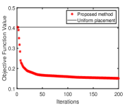
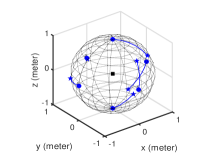
(c) E-optimal design

Figure 3: Convergence plot and corresponding sensor placement for 3D hybrid TOA-RSS under correlated noise. Top: convergence plots; Bottom: sensor placement with black square: target; blue circle: initial sensors’ positions; blue pentagram: final sensors’ positions.

For the 3D case, we have undertaken the design of placing 6 sensors on the surface of sphere of radius $10$ meters with target at its center. The initialization used for our proposed method is given by:

$$\begin{array}[]{ll}\textbf{J}_{\text{uni}}^{T}=\begin{bmatrix}10&0&0&-10&0&0\\ 0&10&0&0&-10&0\\ 0&0&10&0&0&-10\end{bmatrix}.\end{array}$$ (76)

As remarked in the algorithmic section, the proposed method here is only for hybrid TOA-RSS model. The measurements are corrupted with correlated noise of zero-mean and positive definite covariance matrices which are generated similar to the 2D case.

The proposed method is initialized using the uniform placement and the optimal sensor placements are obtained. The variation of objective with iterations are shown in Fig. 3 for all three designs. These plots show monotonic decrease in the objectives which validates the convergence of the proposed algorithm for the 3D case.

IV-C Performance in the presence of uncorrelated noise measurements

Next, we will study the performance of the proposed algorithm for the uncorrelated noise case. To this end, we have assumed that the sensors are to be placed such that the distance from the target (at origin) is always one meter and the measurements are affected by diagonal noise covariance matrices given by:

$$\begin{array}[]{ll}\mathbf{\Sigma}_{\text{TOA}}=\text{diag}[\gamma^{2},\dots,\gamma^{2}]\\ \mathbf{\Sigma}_{\text{RSS}}=\text{diag}[\sigma^{2},\dots,\sigma^{2}]\\ \mathbf{\Sigma}_{\text{AOA}}=\text{diag}[\tau^{2},\dots,\tau^{2}]\end{array}$$ (77)

For the uniform noise case, the optimal orientation matrix satisfies the following relation [40]:

$$\textbf{J}_{*}^{T}\textbf{J}_{*}=\frac{m}{2}\textbf{I}_{n}.$$ (78)

TABLE III: COMPARISON OF THEORETICAL AND NUMERICAL VALUE OF TRACE OF CRLB

No of sensors	$\mathrm{Tr}\left(\mathbf{C}_{\mathrm{theo}}\right)$	$\mathrm{Tr}\left(\mathbf{C}_{\mathrm{algo}}\right)$
2	0.0959	0.0959
5	0.0383	0.0383
10	0.0192	0.0192
15	0.0128	0.0128

The corresponding theoretical value of CRLB can also be easily calculated for this special case using a generalized linear inequality as shown in [43]. This theoretical value is given by:

$$\mathrm{Tr}\left(\mathbf{C}_{\text{theo}}\right)=\frac{4}{\sum\limits_{i=1}^{m}(\frac{\eta^{2}}{d_{i}^{2}\sigma^{2}}+\frac{1}{d_{i}^{2}\tau^{2}}+\frac{1}{\gamma^{2}})}$$ (79)

In the following, we present the value of the trace of CRLB matrix obtained at convergence of our algorithm for different values of ‘$m$’ with the choice of uniform noise variances ($\gamma^{2}=1,\;\sigma^{2}=1,\;\tau^{2}=1$). All the sensor-target ranges are taken to be equal ($d_{i}=1\;\forall i$). The trace of CRLB matrix obtained by the proposed algorithm ($\mathrm{Tr}\left(\mathbf{C}_{\text{algo}}\right)$) and the trace of theoretical CRLB matrix ($\mathbf{\mathrm{Tr}\left(\mathbf{C}_{\text{theo}}\right)}$) using (79) for different number of sensors are listed in table III. From the table, it can be seen that the CRLB value obtained using the proposed algorithm is equivalent to the theoretical CRLB value proving the optimality of the proposed algorithm. The optimal orientation matrix obtained via our algorithm also satisfied the relation in (78).

IV-C1 Optimal design for uniform sensor-target ranges

In this subsection, we assume the distances between the sensors and the target are equal ($d_{i}$$=d$) and generate the optimal orientations for different values of $d$. We have considered two different configuration examples. In example 1, we assume $m=2,\;d=1000\;\mathrm{meter},\;\gamma_{i}=\gamma=1\;\mathrm{meter},\;\sigma_{i}=\sigma=1W,\;\tau_{i}=\tau=1\text{ rad},\;\eta=-4.343$ and the initial positions (used to initialize our algorithm) for the two sensors are taken as $(0.4,-0.7)\text{ kilometers and }(-1,0)$ kilometers. In example 2, we have assumed 3 sensors with initial positions given by $(-0.75,-0.6)\text{ kilometers and }(-1,-0.2)\text{ kilometers}$ and $(0.2,-1)$ kilometers. The initial and final sensors positions (obtained via our proposed algorithm) for example 1 and 2 are shown in Fig. 4. The optimal value of the A optimal objective obtained is $2$ sq. meters and $1.333$ sq. meters which is also the theoretical minimum CRLB value calculated using (79).

Next, we have designed the optimal geometries for different initial positions of the sensors for the parameter settings mentioned in example 1 and 2. The optimal orientations obtained via our proposed approach are shown in Fig. 5 and 6. Some of the optimal configurations obtained via our proposed approach (in Fig 5 and 6) are same as the configurations obtained via the analytical approach of [43].

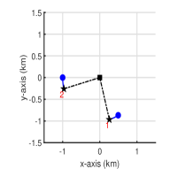
(a)

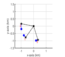
(b)

Figure 4: Optimal sensor trajectories of (a) example 1 and (b) example 2, $\circ:\text{ sensor initial position ,}*:\text{ sensor final position ,}\square:\text{ target position }$

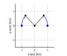
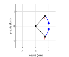
Figure 5: Optimal sensor trajectories and the final geometries with different sensor initial positions for $m=2$ and uniform $d_{i}$ considered in subsection IV-C1 .

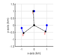
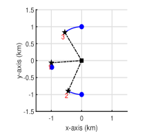
Figure 6: Optimal sensor trajectories and the final geometries with different sensor start positions for $m=3$ and uniform $d_{i}$ considered in subsection IV-C1.

IV-C2 Optimal design for nonuniform sensor-target range

For the analysis of optimal geometry in case of non-uniform $d_{i}$, we have considered design problems of placing 2 and 3 sensors. In the first case, the initial sensor positions and noise variances are taken to be same as in example 1 but the sensor-target ranges are taken to be $d_{1}=2$ kilometers and $d_{2}=1$ kilometers. Similarly, in the second case, the initial sensor positions and noise variances are same as in example 2 but the the sensor-target ranges are taken to be $d_{1}=2$ kilometers, $d_{2}=1$ kilometers and $d_{3}=1.5$ kilometers. The optimal geometries obtained using the proposed algorithm for these examples are given in Fig. 7. The minimum of the A-optimal objective obtained are $1.99$ sq. meters and $1.33$ sq. meters, respectively, which is equal to the minimum theoretical values in (79).

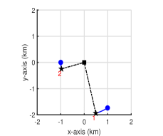
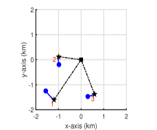
Figure 7: Optimal sensor trajectories and the final geometries for non-uniform $d_{i}$ in example 3 and 4 considered in subsection IV-C2.

IV-D Mean Square Error (MSE) analysis

TABLE IV: COMPARISON OF THE MLE PERFORMANCE FOR DIFFERENT PLACEMENT

No of sensors	Placement	MSE (sq. meters)
	Random	$0.4371$
$m=3$	Uniform	$0.3931$
(uniform noise)	Optimal	$0.1384$
	Random	$0.2763$
$m=5$	Uniform	$0.1417$
(uniform noise)	Optimal	$0.1082$
	Random	$0.5830$
$m=7$	Uniform	$0.0962$
(uniform noise)	Optimal	$0.0867$
	Random	$0.1767$
$m=3$	Uniform	$0.1431$
(non uniform noise)	Optimal	$0.1226$
	Random	$0.0950$
$m=5$	Uniform	$0.0876$
(non uniform noise)	Optimal	$0.0855$
	Random	$0.0886$
$m=7$	Uniform	$0.0803$
(non uniform noise)	Optimal	$0.0771$

Here, we study the improvement in the target localization accuracy using the sensor positions obtained by the proposed approach. We will compare the MSE of the target location obtained using optimal sensor placement given by our approach with the MSE of estimates obtained using the uniform and random sensor placements. The target location estimate is obtained by the maximum likelihood estimation (MLE) approach which is implemented through a 2D grid search of the hybrid likelihood function to arrive at the most probable target location and then performing one step of Gauss-Newton update on the MLE estimate. The configuration used in the simulation is given as follows: The target is considered to be present at $[0,0]^{\text{T}}$ and the sensors are placed on the circumference of circle with unit radius. The uniform and the random sensor geometries are obtained by placing the sensors uniformly and randomly over the circumference, respectively, whereas the optimal geometry is determined using the proposed algorithm. The experiment is conducted for noise measurements which are uncorrelated (with uniform and non-uniform variances). The values of the MSE of the MLE, obtained via 1000 Monte Carlo simulations, are listed in the table IV. From these results, we can observe that the MSE of the estimates in case of optimal placement are smaller than the uniform and random placements.

IV-E Performance analysis of the proposed method for mismatch in the target location estimate

TABLE V: COMPARISON OF THE MLE PERFORMANCE OF SENSOR PLACEMENT FOR TARGET LOCATION MISMATCH

No of sensors	Target Position	MSE (sq. meters)
	True position	$0.1752$
$m=3$	Shifted position 1	$0.1855$
(Uniform noise)	Shifted Position 2	$0.1894$
	True position	$0.0304$
$m=4$	Shifted position 1	$0.0334$
(Non-Uniform noise)	Shifted Position 2	$0.0362$
	True position	$0.0262$
$m=5$	Shifted position 1	$0.0305$
(Non-Uniform noise)	Shifted Position 2	$0.0342$

As discussed in the Remark 2, the optimal sensor placement is designed considering an initial estimate of the target position. However, this initial estimate is very coarse and may not be close to the true target position. So, in this section we study the performance of the proposed algorithm under the mismatch in the target location used in the design. We consider the target position used in the design to be slightly different from the true position. The MSE of the location estimate for the sensor placement obtained by the proposed algorithm is compared with two such cases of target location mismatch. For this, we consider sensors placed on the circumference of a unit circle with target at its center. The measurements are assumed to be corrupted by Gaussian noise. The covariance matrix of the noise is taken to be $\mathbf{I}_{m}$ for uniform noise case and in the case of non-uniform noise, the diagonal elements of it are randomly drawn from uniform distribution of $\mathcal{U}(0,1)$. The target positions used in the design are taken to be $[0.1,-0.2]^{T}$ and $[-0.3,-0.2]^{T}$ for the two mismatched cases. The MSE results for different number of sensors are given in Table V. The MSE for the target mismatch cases are only slightly higher than that for the case which assumes the true target position in the design, this proves the robustness of the design under any mismatch in the design parameters.

V Conclusion and future work

In this paper, a novel MM-based algorithm for optimal sensor placement for a hybrid TOA-RSS-AOA measurement model is proposed. We first derive the design objectives based on A, D and E-optimal criteria, and then reformulate the design problems into saddle-point problems, which are then solved via MM by constructing simple surrogate functions (with closed-from optimizers) over both primal and dual variables. The convergence, estimation efficiency and robustness of the algorithm in designing optimal sensor locations for the hybrid model are verified using various numerical simulations. Unlike the state-of-the-art methods, our proposed algorithm works efficiently for both uncorrelated and correlated noise in the measurements, and as well as for different sensor-target ranges. Furthermore, the MSE for the optimal orientations obtained via our proposed algorithm are found to be smaller than that of the uniform and random placements. As a part of the future work, we would like to model the noise in the measurements to be distance dependent and try and develop a numerical procedure to obtain optimal sensor locations.

Proof of Lemma 3

Proof:

Let us consider the inner minimization problem of (28) over the dual variable $\mathbf{\Phi}$:

$$\min\limits_{\mathbf{\Phi}\succeq 0}~{}\textrm{Tr}[\mathbf{\Phi}\textbf{H}^{T}\textbf{R}\textbf{H}]-\textbf{tr}(\sqrt{\mathbf{\Phi}}).$$ (80)

The Karush-Kuhn-Tucker (KKT) condition for (80) is given by:

$$\textbf{H}^{T}\textbf{R}\textbf{H}-\frac{1}{2}\left(\left(\mathbf{\Phi}^{*}\right)^{-1/2}\right)=\mathbf{0}.$$ (81)

Solving (81), we get the following optimal value:

$$\mathbf{\Phi}^{*}=\frac{1}{4}\left(\textbf{H}^{T}\textbf{R}\textbf{H}\right)^{-2}.$$ (82)

Substituting back $\mathbf{\Phi}^{*}$ in (28), we get:

$$\begin{array}[]{ll}\max\limits_{\textbf{H},\textbf{J}\in\mathcal{D}}~{}-\textrm{Tr}(\frac{1}{4}\textbf{H}^{T}\textbf{R}\textbf{H})^{-1},&\;\textrm{s.t. }\textbf{H}=\begin{bmatrix}\textbf{J}\\ \textbf{J}\textbf{U}\end{bmatrix}.\end{array}$$ (83)

Leaving out the constant $\frac{1}{4}$ and converting (83) into a minimization problem gives the original problem (27). Hence, the equivalence of (27) and (28) is proved. ∎

References

- [1] J. Shen and A. F. Molisch, “Passive location estimation using TOA measurements,” in 2011 IEEE International Conference on Ultra- Wideband (ICUWB), Sept. 2011, pp. 253–257.
- [2] B. Huang, L. Xie, and Z. Yang, “TDOA-based source localization with distance-dependent noises,” IEEE Transactions on Wireless Communications, vol. 14, no. 1, pp. 468–480, Jan. 2015.
- [3] A. Weiss, “On the accuracy of a cellular location system based on RSS measurements,” IEEE Transactions on Vehicular Technology, vol. 52, no. 6, pp. 1508–1518, Nov. 2003.
- [4] K. Ho and W. Xu, “An accurate algebraic solution for moving source location using tdoa and fdoa measurements,” IEEE Transactions on Signal Processing, vol. 52, no. 9, pp. 2453–2463, 2004.
- [5] Y. Zhu, D. Huang, and A. Jiang, “Network localization using angle of arrival,” in 2008 IEEE International Conference on Electro/ Information Technology, May 2008, pp. 205–210.
- [6] K. Panwar, M. Katwe, P. Babu, P. Ghare, and K. Singh, “A majorization-minimization algorithm for hybrid toa-rss based localization in nlos environment,” IEEE Communications Letters, 2022.
- [7] M. Katwe, P. Ghare, P. K. Sharma, and A. Kothari, “NLOS error mitigation in hybrid RSS-TOA-based localization through semi-definite relaxation,” IEEE Commun. Lett., vol. 24, no. 12, pp. 2761–2765, Sep. 2020.
- [8] A. Coluccia and A. Fascista, “Hybrid TOA/RSS range-based localization with self-calibration in asynchronous wireless networks,” Journal of Sensor and Actuator Networks, vol. 8, no. 2, p. 31, 2019.
- [9] S. Tomic and M. Beko, “A robust NLOS bias mitigation technique for RSS-TOA-based target localization,” IEEE Signal Processing Letters, vol. 26, no. 1, pp. 64–68, 2018.
- [10] A. Coluccia and A. Fascista, “On the hybrid TOA/RSS range estimation in wireless sensor networks,” IEEE Transactions on Wireless Communications, vol. 17, no. 1, pp. 361–371, 2017.
- [11] H. Qi, L. Mo, and X. Wu, “SDP relaxation methods for RSS/AOAbased localization in sensor networks,” IEEE Access, vol. 8, pp. 55 113–55 124, 2020.
- [12] S. Chang, Y. Zheng, P. An, J. Bao, and J. Li, “3-D RSS-AOA based target localization method in wireless sensor networks using convex relaxation,” IEEE Access, vol. 8, pp. 106 901–106 909, 2020.
- [13] S. Chang, Y. Li, X. Yang, H. Wang, W. Hu, and Y. Wu, “A novel localization method based on RSS-AOA combined measurements by using polarized identity,” IEEE Sensors Journal, vol. 19, no. 4, pp. 1463–1470, Feb. 2019.
- [14] Q. Qi, Y. Li, Y. Wu, Y. Wang, Y. Yue, and X. Wang, “RSS-AOA-based localization via mixed semi-definite and second-order cone relaxation in 3-D wireless sensor networks,” IEEE Access, vol. 7, pp. 117 768– 117 779, 2019.
- [15] S. Tomic, M. Beko, and M. Tuba, “A linear estimator for network localization using integrated RSS and AOA measurements,” IEEE Signal Processing Letters, vol. 26, no. 3, pp. 405–409, 2019.
- [16] V. Y. Zhang, A. K.-s. Wong, K. T. Woo, and R. W. Ouyang, “Hybrid TOA/AOA-based mobile localization with and without tracking in CDMA cellular networks,” in 2010 IEEE Wireless Communication and Networking Conference. IEEE, 2010, pp. 1–6.
- [17] J. Yin, Q. Wan, S. Yang, and K. Ho, “A simple and accurate TDOAAOA localization method using two stations,” IEEE Signal Processing Letters, vol. 23, no. 1, pp. 144–148, 2015.
- [18] Y. Wang and K. C. Ho, “Unified near-field and far-field localization for AOA and hybrid AOA-TDOA positionings,” IEEE Transactions on Wireless Communications, vol. 17, no. 2, pp. 1242–1254, Feb. 2018.
- [19] T. Jia, H. Wang, X. Shen, Z. Jiang, and K. He, “Target localization based on structured total least squares with hybrid TDOA-AOA measurements,” Signal Processing, vol. 143, pp. 211–221, 2018.
- [20] N. H. Nguyen and K. Dogancay, “Multistatic pseudolinear target motion analysis using hybrid measurements,” Signal Processing, vol. 130, pp. 22–36, Jan. 2017.
- [21] H. Seo, H. Kim, J. Kang, I. Jeong, W. Ahn, and S. Kim, “3D moving target tracking with measurement fusion of TDOA/FDOA/AOA,” ICT Express, vol. 5, no. 2, pp. 115–119, 2019.
- [22] A. N. Bishop, B. Fidan, B. D. Anderson, K. Dogancay, and P. N. Pathirana, “Optimality analysis of sensor-target localization geometries,” Automatica, vol. 46, no. 3, pp. 479–492, 2010.
- [23] K. Yoo, J. Chun, and C. Ryu, “CRB-based optimal radar placement for target positioning,” in 2018 International Conference on Radar (RADAR), Aug. 2018, pp. 1–5.
- [24] K. Yoo and J. Chun, “Analysis of optimal range sensor placement for tracking a moving target,” IEEE Communications Letters, vol. 24, no. 8, pp. 1700–1704, May 2020.
- [25] J. Fawcett, “Effect of course maneuvers on bearings-only range estimation,” IEEE Transactions on Acoustics, Speech, and Signal Processing, vol. 36, no. 8, pp. 1193–1199, Aug. 1988.
- [26] D. Ucinski, Optimal measurement methods for distributed parameter system identification. CRC press, 2004.
- [27] Y. Oshman and P. Davidson, “Optimization of observer trajectories for bearings-only target localization,” IEEE Transactions on Aerospace and Electronic Systems, vol. 35, no. 3, pp. 892–902, 1999.
- [28] B. Yang and J. Scheuing, “Cramer-Rao bound and optimum sensor array for source localization from time differences of arrival,” in Proceedings. (ICASSP ’05). IEEE International Conference on Acoustics, Speech, and Signal Processing, 2005., vol. 4, May 2005.
- [29] D. Moreno-Salinas, A. Pascoal, and J. Aranda, “Optimal sensor placement for acoustic underwater target positioning with range-only measurements,” IEEE Journal of Oceanic Engineering, vol. 41, no. 3, pp. 620–643, 2016.
- [30] D. Moreno-Salinas, A. M. Pascoal, and J. Aranda, “Optimal sensor placement for multiple target positioning with range-only measurements in two-dimensional scenarios,” Sensors, vol. 13, no. 8, pp. 10 674–10 710, 2013.
- [31] A. Heydari, M. Aghabozorgi, and M. Biguesh, “Optimal sensor placement for source localization based on RSSD,” Wireless Networks, vol. 26, pp. 5151–5162, 2020.
- [32] N. H. Nguyen and K. Dogancay, “Optimal geometry analysis for multistatic TOA localization,” IEEE Transactions on Signal Processing, vol. 64, no. 16, pp. 4180–4193, Aug. 2016.
- [33] N. Nguyen and K. Dogancay, “Optimal sensor placement for doppler shift target localization,” in 2015 IEEE Radar Conference (RadarCon), 2015, pp. 1677–1682.
- [34] L. Rui and K. C. Ho, “Elliptic localization: Performance study and optimum receiver placement,” IEEE Transactions on Signal Processing, vol. 62, no. 18, pp. 4673–4688, 2014.
- [35] K. Dogancay and H. Hmam, “Optimal angular sensor separation for AOA localization,” Signal Processing, vol. 88, no. 5, pp. 1248–1260, May 2008.
- [36] S. Xu and K. Dogancay, “Optimal sensor placement for 3-D angle-ofarrival target localization,” IEEE Trans. Aerosp. Electron. Syst., vol. 53, no. 3, pp. 1196–1211, Jun. 2017.
- [37] S. Xu, Y. Ou, and W. Zheng, “Optimal sensor-target geometries for 3-D static target localization using received-signal-strength measurements,” IEEE Signal Processing Letters, vol. 26, no. 7, pp. 966–970, Jul. 2019.
- [38] S. Xu, Y. Ou, and X. Wu, “Optimal sensor placement for 3-D time-ofarrival target localization,” IEEE Transactions on Signal Processing, vol. 67, no. 19, pp. 5018–5031, Oct. 2019.
- [39] N. H. Nguyen, “Optimal geometry analysis for target localization with bayesian priors,” IEEE Access, vol. 9, pp. 33 419–33 437, Feb. 2021.
- [40] N. Sahu, L. Wu, P. Babu, B. Shankar, and B. Ottersten, “Optimal sensor placement for source localization: A unified admm approach,” IEEE Transactions on Vehicular Technology, pp. 1–1, 2022.
- [41] H. Hmam, “Optimal sensor velocity configuration for TDOA-FDOA geolocation,” IEEE Transactions on Signal Processing, vol. 65, no. 3, pp. 628–637, 2017.
- [42] W. Wang, P. Bai, Y. Wang, X. Liang, and J. Zhang, “Optimal sensor deployment and velocity configuration with hybrid TDOA and FDOA measurements,” IEEE Access, vol. 7, pp. 109 181–109 194, 2019.
- [43] S. Xu, “Optimal sensor placement for target localization using hybrid RSS, AOA and TOA measurements,” IEEE Communications Letters, vol. 24, no. 9, pp. 1966–1970, Sept. 2020.
- [44] S. P. Robinson, P. A. Lepper, and R. A. Hazelwood, “Good practice guide for underwater noise measurement.” 2014.
- [45] A. Coluccia and F. Ricciato, “RSS-based localization via Bayesian ranging and iterative least squares positioning,” IEEE Communications Letters, vol. 18, no. 5, pp. 873–876, May 2014.
- [46] S. M. Kay, Fundamentals of statistical signal processing: estimation theory. Prentice-Hall, Inc., 1993.
- [47] Y. Sun, P. Babu, and D. P. Palomar, “Majorization-minimization algorithms in signal processing, communications, and machine learning,” IEEE Transactions on Signal Processing, vol. 65, no. 3, pp. 794–816, 2016.
- [48] S. Boyd and L. Vandenberghe, Convex optimization. Cambridge university press, 2004.
- [49] M. Sion, “On general minimax theorems,” Pacific Journal of mathematics, vol. 8, no. 1, pp. 171–176, 1958.
- [50] E. H. Lieb, “Convex trace functions and the wigner-yanase-dyson conjecture,” Les rencontres physiciens-mathématiciens de Strasbourg- RCP25, vol. 19, pp. 0–35, 1973.
- [51] I. Pólik and T. Terlaky, “Interior point methods for nonlinear optimization,” in Nonlinear optimization. Springer, 2010, pp. 215–276.